BOTTOM SCHUR FUNCTIONS
Peter Clifford
CNRI,
Dublin Institute of Technology,
Ireland
peterc@alum.mit.edu
Richard P. Stanley 11
1
Partially supported by NSF grant
#DMS-9988459.
Department of Mathematics, Massachusetts Institute of
Technology
Cambridge, MA 02139, USA
rstan@math.mit.edu
Submitted: Nov 19, 2003; Accepted 27 Aug, 2004
MR Subject Classifications: 05E05, 05E10
Abstract
We give a basis for the space spanned by the sum of the lowest degree terms in the expansion of the Schur symmetric functions in terms of the power sum symmetric functions , where deg. These lowest degree terms correspond to minimal border strip tableaux of . The dimension of the space spanned by , where is a partition of , is equal to the number of partitions of into parts differing by at least 2. Applying the Rogers-Ramanujan identity, the generating function also counts the number of partitions of into parts and .
We also show that a symmetric function closely related to has the same coefficients when expanded in terms of power sums or augmented monomial symmetric functions.
1 Introduction
Let be a partition of the integer , i.e., and . The length of a partition is the number of nonzero parts of . The (Durfee or Frobenius) rank of , denoted rank(), is the length of the main diagonal of the diagram of , or equivalently, the largest integer for which . The rank of is the least integer such that is a disjoint union of border strips (defined below).
Nazarov and Tarasov [1, Sect. 1], in connection with tensor products of Yangian modules, defined a generalization of rank to skew partitions (or skew diagrams) . The paper [3, Proposition 2.2] gives several simple equivalent definitions of rank(). One of the definitions is that rank() is the least integer such that is a disjoint union of border strips. It develops a general theory of minimal border strip tableaux of skew shapes, introducing the concepts of the snake sequence and the interval set of a skew shape . These tools are used to count the number of minimal border strip decompositions and minimal border strip tableaux of . In particular, the paper [3] gives an explicit combinatorial formula for the coefficients of the , where , which appear in the expansion of .
The paper [3] considered a degree operator deg and defined the bottom Schur functions to be the sum of the terms of lowest degree which appear in the expansion of as a linear combination of the . We study the bottom Schur functions in detail when . In particular, in Section 4 we give a basis for the vector space they span.
In Section 7 we show that when we substitute for in the expansion of a bottom Schur function in terms of power sums, then the resulting symmetric function has the same coefficients when expanded in terms of power sums or augmented monomial symmetric functions.
2 Definitions
In general we follow [2, Ch. 7] for notation and terminology involving symmetric functions. Let be a partition of with Frobenius rank . Recall that is the length of the main diagonal of the diagram of , or equivalently, the largest integer for which . Let , the number of parts of equal to . Define . A border strip (or rim hook or ribbon) is a connected skew shape with no square. An example is whose diagram is illustrated in Figure 1. Define the height ht() of a border strip to be one less than its number of rows.

Let be a weak composition of , i.e., and . Define a border strip tableau of shape and type to be an assignment of positive integers to the squares of such that:
- (a)
every row and column is weakly increasing,
- (b)
the integer appears times, and
- (c)
the set of squares occupied by forms a border strip.
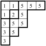
Equivalently, one may think of a border-strip tableau as a sequence of partitions such that each skew shape is a border-strip of size . For instance, Figure 2 shows a border strip tableau of of type .
It is easy to see (in this nonskew case) that the smallest number of strips in a border-strip tableau is rank(). Define the height ht() of a border-strip tableau to be
where are the (nonempty) border strips appearing in . In the example we have ht. Now we can define
summed over all border-strip tableaux of shape and type . Since there are at least rank strips in every tableau, we have that if rank. The numbers for are the values of the irreducible characters of the symmetric group .
Finally we can express the Schur function in terms of power sums , viz.,
| (2.1) |
Define deg() , so deg(. The bottom Schur function is defined to be the lowest degree part of , so
Also write . For instance,
Hence
We identify a partition with its diagram
Let be an edge of the lower envelope of , i.e., no square of has as its upper or left-hand edge. We will define a certain subset of squares of , called a snake. If is horizontal and is the square of having as its lower edge, define
| (2.2) | |||||
If is vertical and is the square of having as its right-hand edge, define
| (2.3) | |||||
In Figure 3 the nonempty snakes of the shape are shown with dashed paths through their squares, with a single bullet in the two snakes with just one square. The length of a snake is one fewer than its number of squares; a snake of length (so with squares) is call an i-snake. Call a snake of even length a left snake if is horizontal and a right snake if is vertical. It is clear that the snakes are linearly ordered from lower left to upper right. In this linear ordering, replace a left snake with the symbol , a right snake with , and a snake of odd length with . The resulting sequence (which does not determine ) is called the snake sequence of , denoted SS. For instance, from Figure 3 we see that

Lemma 2.1.
The ’s in the snake sequence correspond exactly to horizontal edges of the lower envelope of which are below the line . The ’s correspond exactly to vertical edges of the lower envelope of which are above the line . All other edges of the lower envelope of are labelled by ’s.
Clearly we could have defined the snake sequence this way; however, the definitions above also hold for skew shapes. Lemma 2.1 only holds when is a straight (i.e., nonskew) shape.
Proof.
Let be an edge of the lower envelope of below the line . Let be the square of having as its lower edge. The last square in the snake is some square in the first column of . So if is horizontal then the last square is , the snake has an odd number of squares and so has even length, and is labelled by . If is vertical then the last square is , the snake has an even number of squares, so has odd length, and is labelled by . The case when is above is proved similarly. ∎
Corollary 2.2.
In the snake sequence of , the ’s occur strictly to the left of the ’s.
The number of horizontal edges of the lower envelope of which are below the line equals the length of the main diagonal of the diagram of , which is the rank of . Similarly the number of vertical edges of the lower envelope of which are above the line also equals the rank of . Henceforth we fix .
Let SS, and define an interval set of to be a collection of ordered pairs,
satisfying the following conditions:
- (a)
the ’s and ’s are all distinct integers,
- (b)
,
- (c)
and .
Figure 4 illustrates the interval set of the shape 533322.

Given an interval set , define the crossing number to be the number of crossings of , i.e. the number of pairs for which .
Let be a border strip tableau of shape . Recall that
where ranges over all border strips in and is one less than the number of rows of . Define to be the height of a “greedy border strip tableau” of shape obtained by starting with and successively removing the largest possible border strip. (Although may not be unique, the set of border strips appearing in is unique, so is well-defined.)
The connection between bottom Schur functions and interval sets was given by Stanley [3, Theorem 5.2]:
where ranges over all interval sets of .
For example the shape has snake sequence . There are two interval sets, with crossing number , and with crossing number . So as we saw before
3 Bottom Schur Functions of straight shapes
Lemma 3.1.
The lexicographic order on shapes whose length equals their rank is equal to the reverse lexicographical order (with respect to the ordering LRO) on their snake sequences.
Proof.
Since , the snake sequence begins with L’s. If the length of the th row of is , then there are O’s to the left of the st R. ∎
Denote the complete homogeneous symmetric functions by . Recall that the Jacobi-Trudi identity expresses the ’s in terms of the ’s:
where we define for . For example
Since , the term of lowest degree (in ) in the expansion of a given in terms of the is just . For a product the term of lowest degree in the expansion in terms of the is just . So we have that terms of lowest order in (since the are algebraically independent, and since , this determinant will not vanish). For example
Since , the terms of lowest order are those which contain the most number of 1’s.
Row of the matrix will have a in position if , i.e. if (this shows that the number of rows of which do not contain a is another definition of [3, Prop. 2.2]).
Let be the matrix obtained from the original Jacobi-Trudi matrix by removing every row and column which contains a 1 and replacing the with . We show below that this matrix is not singular and so we have
For example
Any minor of the Jacobi-Trudi matrix for a shape is the Jacobi-Trudi matrix for some skew shape . For let be some minor of size of some Jacobi-Trudi matrix . If the entry in position is put . Now we can set
and
Again note that since the are algebraically independent and , we have .
In our running example, we have and . Hence . Also and . Thus . Therefore we have that equals the determinant of the Jacobi-Trudi matrix of with the ’s replaced by ’s.
Lemma 3.2.
If the skew shape has the Jacobi-Trudi matrix obtained by removing all rows and columns with a 1 from a Jacobi-Trudi matrix of a shape with rank , then contains a square of size .
The rank of is , and the diagram of does indeed contain a square of size 4:
![[Uncaptioned image]](0311382v2/77662210.png)
Proof.
We give a proof due to Christine Bessenrodt, greatly improving our original proof. Define and . We give a diagrammatic definition of and which also illustrates that the skew diagram contains a square of size . Consider as a square with two partitions and glued to it, i.e. . Flip over its anti-diagonal and then glue the bottom right corner of the result to the bottom left corner of the square. The final diagram is the skew diagram of . We show that and .
The rows of are contained in the first rows of , so for some constant . The last column of does not have a 1 in it, so it will not be removed, and its first entries will be the last column of . Hence . Since , we have .
The first entries of the last column of are retained. Then we remove the next columns to its left, do not remove the next column, remove the next columns to the left, and so on. Formally we have . Combining this with gives us .
∎
4 The space spanned by the bottom Schur functions
Before we use the above results to give a basis for the space spanned by the bottom Schur functions, we must first recall some classical tableaux theory.
If is a skew shape, then a standard Young tableau (SYT) of shape is a labelling of the squares of with the numbers , each number appearing once, so that every row and column is increasing. A semistandard Young tableau (SSYT) of shape is a labelling of the squares of with positive integers that is weakly increasing in every row and strictly increasing in every column. We say that has type if has parts equal to .
![[Uncaptioned image]](0311382v2/sytssyt.png)
Now we define an operation (of Schützenberger) on standard Young tableaux called a jeu de taquin slide. Given a skew shape , consider the squares that can be added to , so that shares at least one edge with , and is a valid skew shape. Suppose that shares a lower or right edge with (the other situation is completely analogous). There is at least one square in that is adjacent to ; if there are two such squares, then let be the one with a smaller entry. Move the entry occupying into . Then repeat this procedure, starting at . The resulting tableau will be a standard Young tableau. Analogously if shares an upper or left edge, the operation is the same except we let be the square with the bigger entry from two possibilities. For example we illustrate both situations in Figure 5; the tableau on the right results from playing jeu de taquin beginning at the square marked by a bullet on the tableau on the left (and vice versa).

Two tableaux and are called jeu de taquin equivalent if one can be obtained from another by a sequence of jeu de taquin slides. Given an SYT of shape , there is exactly one SYT of straight shape, denoted jdt, that is jeu de taquin equivalent to [2, Thm. A1.2.4].
The reading word of a (semi)standard Young tableau is the sequence of entries of obtained by concatenating the rows of bottom to top. For example, the tableau on the left in Figure 5 has the reading word . The reverse reading word of a tableau is simply the reading word read backwards.
A lattice permutation is a sequence such that in any initial factor , the number of ’s is at least as great as the number of ’s (for all ). For example is a lattice permutation.
The Littlewood-Richardson coefficients are the coefficients in the expansion of a skew Schur function in the basis of Schur functions:
The Littlewood-Richardson rule is a combinatorial description of the coefficients . We will use two different versions of the rule.
Theorem 4.1 (Schützenberger, Thomas).
Fix an SYT of shape . The Littlewood-Richardson coefficient is equal to the number of SYT of shape that are jeu de taquin equivalent to .
![[Uncaptioned image]](0311382v2/tableaup.png)
For example, let and . Consider the tableau of shape shown above. There are exactly two SYTs of shape such that , namely,
![[Uncaptioned image]](0311382v2/twosyts.png)
Theorem 4.2 (Schützenberger, Thomas).
The Littlewood-Richardson coefficient is equal to the number of semistandard Young tableaux of shape and type whose reverse reading word is a lattice permutation.
For example, with and as above, there are exactly two SSYTs of shape and type whose reverse reading word is a lattice permutation:
![[Uncaptioned image]](0311382v2/lrtableaux.png)
Now we have enough machinery to state and prove this section’s main theorem.
Theorem 4.3.
Fix and . The set and is a basis for the space .
For example if and , we have that is a basis for .
Proof.
First we prove that the are linearly independent. We show that given any such , there is some term in the expansion of which does not occur in the expansion of any for lexicographically less than .
From [3, Theorem 5.2] we have that
where ranges over all interval sets of . Let be the term corresponding to the noncrossing interval set of the snake sequence of . We claim that does not occur in the expansion of any for lexicographically less than . Assume by way of contradiction that it does occur for some such with corresponding interval set .
Assume inductively that the first L’s are matched with the last R’s without crossings in . Let (and respectively) be the position of the th R in the snake sequence of ( respectively). By Lemma 3.1 . But the length of the interval matching the th R from the right in is . So for there to be an interval of this length in we must match the th R from the right with the th L; this interval has no crossing. Proceeding by induction we see that is also noncrossing, and so must equal . This shows that the snake sequences corresponding to and are equal. Identical snake sequences and equal lengths guarantee that , a contradiction.
Now we prove that the span the space of all . We have shown that . Expand in terms of (straight) Schur functions using the Littlewood Richardson rule
We need to show that unless is of rank and length .
Fix an SYT P of shape . The Littlewood-Richardson coefficient is equal to the number of SYT of shape that are jeu de taquin equivalent to P. Playing jeu de taquin on a straight-shape tableau of shape can only increase the length of the shape. Hence if .
The Littlewood-Richardson coefficient is also equal to the number of semistandard Young tableaux of shape and type whose reverse reading word is a lattice permutation. But we know that contains a square of size (by Lemma 3.2). Therefore the bottom boxes of this square must have labels at least . Since , the labels are exactly . So , i.e. rank(. Since , we must have rank(.
Taking terms of lowest degree on both sides of
we have that
where the sum is over of length and rank as required. ∎
5 Dimension of the space spanned by the bottom Schur functions
Let be the number of partitions of with length at most , and define . A partition of length and rank decomposes into a square of boxes and a partition of of length at most .
Corollary 5.1.
The dimension of the space of bottom Schur functions
is
For example, the first 27 terms in this sequence (beginning with ) are
There is a nice bijection between the above partitions and the set of partitions . For, given a and a partition with fewer than parts, we can set . This gives a partition of with rows with as required. This is clearly a bijection.
This classical sequence also gives the number of partitions of into parts congruent to or ; equivalently these numbers are the coefficients in the expansion of the Rogers-Ramanujan identity
6 2-bottom Schur functions
We have shown that a basis for the space spanned by the bottom Schur functions consists of the where . It is natural to define for fixed the -bottom Schur function to be the sum of those terms of degree at most rank in the expansion (2.1) (with as usual). When we have verified (using Stembridge’s SF package for Maple [4]) that for the dimension of the space spanned by equals the number of satisfying . This suggests the following conjecture.
Conjecture 6.1.
A basis for the space spanned by the 2-bottom Schur functions consists of all 2-bottom Schur functions , where is a partition of n satisfying .
However in the case, the dimensions of the spaces spanned by the 3-bottom Schur functions are . We have computed that the numbers of satisfying are given by . Unfortunately these sequences do not agree.
7 A condition satisfied by bottom Schur functions
We prove a surprising identity satisfied by a variant of the bottom Schur functions related to their expansion in terms of power sum and monomial symmetric functions.
Fix a shape of rank . Given an interval set of and a labelling of the intervals such that , define
Recall that is the number of crossings of the interval set . Figure 6 shows a labelled interval set of the shape 533322 with the snake sequence . For this interval set and for this labelling .

Example 7.1.
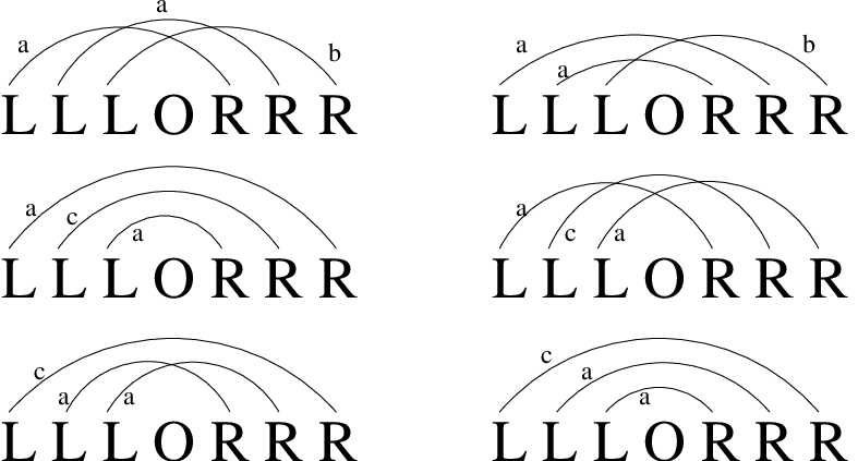
For the shape with snake sequence , Figure 7 depicts some of the labelled interval sets. In the top left we have . In the top right we have . In fact in every row the term in the left column is exactly the negative of the corresponding term in the right column.
Lemma 7.1.
Fix a shape . Then , where the sum is over all labelled interval sets of with at least one label repeated.
Proof.
We give a sign reversing involution on these labelled interval sets. Examine a specific labelled interval set . Since we are dealing with straight (non-skew) shapes, we know by Corollary 2.2 that the snake sequence has all the L’s before any of the R’s, or . So any two intervals and ( say) either intersect () or are nested ().
Let be the smallest label which is repeated. The intervals in are ordered by where they start, so identifying the first two intervals and () labelled by is well-defined.
Simply change the interval to and the interval to , while preserving the label on both. Where the intervals start remains unchanged, so these intervals remain the first two intervals labelled by . Hence this operation is an involution. Note that if the two intervals initially nested, they now intersect, and if they initially intersected, they now nest. The parity of the number of crossings of these two with any other interval is preserved under this operation. So the parity of the total number of crossings has changed, and this involution is sign reversing. The rows of Figure 7 are some examples of this involution (if ).
Thus given any labelled interval set with repeated labels, there is a unique labelled interval set with one more (or fewer) crossings, and so the sum of all such terms is zero. ∎
Fix a shape . Recall that
where ranges over all interval sets of .
For another shape , define to be the coefficient of in the above sum, i.e.
where the sum is over all interval sets (of ) of type .
Lemma 7.2.
, where the sum is over all labelled interval sets of type .
Example 7.2.
Consider as before the shape with snake sequence . In particular, consider the interval set of type labelled by . This interval set is illustrated in Figure 8. If then and the sum over all such labellings will give . If the sum over all such labellings will give . Similarly if we will get , and if we will get . Finally if the three labels are all different, the sum will give . So the sum over all such labellings is .

Proof.
We need to show that for every interval set of type , , where the sum is over all labellings of . First note that the intervals can be ordered largest first and left to right among intervals of the same length. So the th interval is well defined, and has length .
By definition . But if we expand this product into monomials , each monomial corresponds uniquely to the labelling of where the th interval is labelled by , and so occurs exactly once in as required. ∎
The augmented monomial symmetric function is defined by
where denotes a monomial symmetric function.
Lemma 7.3.
, where the sum is over all labelled interval sets of of type with no label repeated.
Note that we have already demonstrated this result in Example 7.2. Indeed for that interval set when the labels were all different we saw that .
Proof.
Fix a specific interval set of type . We need to show where the sum is over all labellings with no label repeated. As before we can order the intervals and say that the th interval is labelled by . Note that if , the two labellings and both produce the same term . So we have where we impose the condition that if , then . Recall that by definition. So we have as required. ∎
Theorem 7.4.
For each shape , write the bottom Schur function . Then .
Example 7.3.
For we have
So our result states that
Proof.
Let denote the space of all symmetric functions with rational coefficients such that if , then
Theorem 7.4 shows that . However, there are elements of that are not linear combinations of ’s, such as . Let denote the transition matrix from monomial symmetric functions to the power sums, i.e.,
Let denote the diagonal matrix whose diagonal coincides with that of , so
It is easy to see that , the kernel (or null space) of . Let denote the elements of that are homogeneous of degree , and let . We have computed that
Compare this with the dimension of the space spanned by the bottom Schur functions of degree , given in general by Corollary 5.1 and for just below this corollary. In particular, the least for which is . We don’t have a conjecture for the value of .
References
- [1] M. Nazarov and V. Tarasov, On irreducibility of tensor products of Yangian modules, Internat. Math. Research Notices (1998), 125-150.
- [2] R. P. Stanley, “Enumerative Combinatorics,” Vol. 2, Cambridge Univ. Press, New York/Cambridge, UK, 1999.
- [3] R. P. Stanley, The Rank and Minimal Border Strip Decompositions of a Skew Partition, J. Combin. Theory (A) 100 (2002), 349-375.
- [4] J. R. Stembridge, The SF Package for Maple, Version 2.3, 22 July 2001, http://www.math.lsa.umich.edu/jrs/maple.html#SF