Teichmüller curves, Galois actions and $\widehat{GT}$-relations

Consider a complex geodesic for the Teichmüller metric $\tilde{\char 17\relax}:\mathbb{H}\to T_{g}$ from the upper half plane to Teichmüller space. These geodesics are generated by a pair $(X,q)$ of a Riemann surface $X$ of genus $g$ and a quadratic differential $q$. The (rare) examples where the stabilizer in the mapping class group of $\tilde{\char 17\relax}$ is a lattice $\Gamma\subset{\rm Aut}(\mathbb{H})$ are called Teichmüller curves.

A particular case of these geodesics with lattice stabilizer can be described as follows: Take an assemblage of squares of paper and glue them along their edges to a surface without boundary, such that at each vertex abut an even number of squares. If we provide the squares with a complex structure and glue the local quadratic differentials $dz^{2}$, we obtain a pair $(X,q)$.
This description lead Lochak ([11]) to baptise them origamis. If the glueing is just by translations (and not by $(-1)$ composed by a translation) the origami is said to be oriented. Oriented origamis are also known as square-tiled coverings or non-primitive Teichmüller curves. Lochak remarked that the corresponding origami curves $j:C=\mathbb{H}/\Gamma\to M_{g}$ in the moduli space of curves are defined over number fields and hence interesting not only in dynamical systems but also from a number theoretical viewpoint.
We study two examples (section 4) of origamis: the smallest example (called $L(2,2)$) where $X$ has genus greater than one and the smallest example (called ${\mathcal{S}}_{2}$) with a property relevant for the $\widehat{GT}$-comparisons, see below. In both cases we explicitly write down the equation of the origami curve in moduli space. This possibility seems rather unexpected from the ’geodesic’ viewpoint.

The above definition suggests that – in the oriented case – origami curves are in fact (the analytic version of) some Hurwitz spaces for coverings of elliptic curves, ramified at most over $\infty$. It is very natural to consider the geodesic discs then in $M_{g,[n]}$ with the $n$ preimages of $\infty$ marked but unordered. The Hurwitz viewpoint reproves that origami curves and the map $j$ are defined over number fields. It implies that there is an action of the absolute Galois group $G_{\mathbb{Q}}$ on the set of origami curves. Our first main result is that this action is faithful in the following sense (we abbreviate $\mathbb{P}^{1}\smallsetminus\{0,1,\infty\}$ by $\mathbb{P}^{*}$ throughout):

Theorem 5.4 For each $\sigma\in G_{\mathbb{Q}}$ there is an origami curve $C$ isomorphic to $\mathbb{P}^{*}$, such that $\sigma$ acts non-trivially on the map $j(C)\to M_{g,[n]}$, more precisely such that $j(C)\neq j^{\sigma}(C)$.

There are examples of origami curves, that do not have genus $0$. ([20]). It would be interesting to know, if the $G_{\mathbb{Q}}$-action is faithful on the (abstract, not embedded) origami curves.

Let us give an overview over Grothendieck-Teichmüller theory. The technical details will be explained in section 6.
The absolute Galois group $G_{\mathbb{Q}}$ acts on the algebraic fundamental group $\pi_{1}(\mathbb{P}^{\ast}_{\overline{\mathbb{Q}}})$, which is isomorphic to the profinite free group $\widehat{F_{2}}$ in two generators. This action can be described in terms of pairs $(\lambda_{\sigma},f_{\sigma})\in\widehat{\mathbb{Z}}\times(\widehat{F_{2}})^{\prime}$ with a suitable composition law. The subgroup of pairs satisfying three equations (due to Drinfel’d) is the Grothendieck-Teichmüller group $\widehat{GT}$. By construction it contains $G_{\mathbb{Q}}$ and the question is whether it is strictly larger than $G_{\mathbb{Q}}$ or not. One hence would like to find a set of equations that singles out precisely $G_{\mathbb{Q}}$.
Where should these relations come from? Consider a category ${\mathcal{C}}$ of varieties (or stacks) over $\mathbb{Q}$ with some morphisms defined over $\mathbb{Q}$. For a large enough ${\mathcal{C}}$ only $G_{\mathbb{Q}}$ acts equivariantly on all $\pi_{1}({\mathcal{C}})$ by a result of F. Pop.
But only for a few types of ’geometric’ morphisms one is able to express the equivariance in terms of $(\lambda,f)$. Among these are some coverings of curves ([17], [18]), and ’natural’ morphisms between moduli spaces of curves ([5], [17], [22]). Maps from curves to moduli spaces should be considered next.
The map of some origami curves to moduli space are defined over $\mathbb{Q}$ and ’geometric’ in this sense. We need that the curve $C\cong\mathbb{P}^{*}$ and that it passes through a maximally degenerate point of the (compactified) moduli space. The smallest such origami is the ${\mathcal{S}}_{2}$.
Let $\alpha_{1},\ldots,\alpha_{5}$ denote the standard generators (see section 7) of the profinite mapping class group $\widehat{\Gamma_{2,0}}$. For $\sigma\in G_{\mathbb{Q}}$ such that the Kummer cocycle $\rho_{2}(\sigma)=0$ we obtain the following relation:

Theorem 7.1’ The element $(\lambda,f)\in\widehat{GT}$ respects the Galois actions on the morphism $j:C^{\rm orb}\to{\mathcal{M}}_{2}$ induced from the two-steps origami ${\mathcal{S}}_{2}$ (see figure $4$) if and only if

holds in $\widehat{\Gamma_{2,0}}$. The elements $(\lambda,f)$ satisfying this relation form a subgroup of $\widehat{GT}$ containing $G_{\mathbb{Q}}$.

In section 7 we prove the refined relation for all $G_{\mathbb{Q}}$. As for all the relations in $\widehat{GT}$ recently discovered it is not known, if the subgroup defined by this relation is properly between $G_{\mathbb{Q}}$ and $\widehat{GT}$.

The author thanks Pierre Lochak and Leila Schneps a lot for introducing him to this subject and a lot of support. He also thanks W. Herfort and H. Nakamura for their suggestions.

A holomorphic quadratic differential $q\neq 0$ on a Riemann surface $X$ of genus $g$ determines on $X$ minus the set of zeroes of $q$ an atlas of open charts, whose transition functions are of the form $z\mapsto\pm z+c$. Such an atlas is called a flat structure on $X$. Conversely a flat structure determines a quadratic differential by glueing the local $dz^{2}$’s. This correspondence is given in more details in [11] Ch. 2.
15:58 There is a natural ${\rm SL}_{2}(\mathbb{R})$ action on pairs $(X,q)$ by postcomposing the charts of the flat structure with the linear map. The stabilizer of a pair $(X,q)$ is precisely ${\rm SO}_{2}(\mathbb{R})$. We define the Teichmüller space ${\mathcal{T}}_{g}$ as the space of Riemann surfaces plus an isotopy class of orientation-preserving diffeomorphism (a Teichmüller marking) to a reference surface $\Sigma_{g}$. If we choose a Teichmüller marking on $X$, the action ${\rm SL}_{2}(\mathbb{R})\cdot(X,q)$ yields a geodesic curve (by Teichmüller’s theorems) $\tilde{\char 17\relax}:\mathbb{H}\to{\mathcal{T}}_{g}$. We denote by ${\mathcal{M}}_{g}$ the moduli stack of curves and the corresponding coarse moduli space by non-calligraphic letters, i.e. $M_{g}$.

Consider the projection of a geodesic $\mathbb{H}\to{\mathcal{T}}_{g}$ to $M_{g}$. We consider the moduli space in the first two sections in the analytic category. More precisely we should write $(M_{g})_{\mathbb{C}}^{{\rm an}}$, etc. Let $\Gamma_{g,n}$ be the mapping class group of Riemann surfaces of genus $g$ with $n$ punctures. We define ${\rm Stab}(\tilde{\char 17\relax})\subset\Gamma_{g,0}$ to be the (setwise) stabilizer of $\tilde{\char 17\relax}(\mathbb{H})$ and ${\rm Aut}(\tilde{j})$ to be the pointwise stabilizer. We summarize this by an exact sequence

The map $\tilde{\char 17\relax}$ descends to a map

Later on it will sometimes be natural to fix say $n$ marked points, consider $\tilde{\char 17\relax}:\mathbb{H}\to{\mathcal{T}}_{g,n}$ and consider the stabilizer in $\Gamma_{g,n}$ (or in $\Gamma_{g,[n]}$, if we allow permutation of the marked points). We then call the groups ${\rm Stab}(\tilde{\char 17\relax},n)$ (or ${\rm Stab}(\tilde{\char 17\relax},[n])$) etc.

We can also describe this group using the flat structure defined by $(X,q)$. Denote by ${\rm Aff}^{+}(X,q)$ the group of orientation preserving affine diffeomorphisms of $X$, i.e. diffeomorphisms which are affine with respect to the charts of the flat structure determined by $q$. Associating with $\varphi\in{\rm Aff}^{+}(X,q)$ the matrix part of the affine maps yields a well-defined map $D$ to ${\rm PSL}_{2}(\mathbb{R})$. We denote the image of $D$ by ${\rm PSL}(X,q)$. We obtain an exact sequence

where ${\rm Aut}(X,q)$ are the (conformal) automorphisms of $X$ preserving $q$.

We will also consider the subgroup of ${\rm Aff}^{+}(X,q)$ that fixes $n$ points (resp. up to permutation). We will denote these groups by ${\rm Aff}^{+}(X,q,n)$ (resp. ${\rm Aff}^{+}(X,q,[n])$) and their images under $D$ by ${\rm PSL}(X,q,n)$ (resp. ${\rm PSL}(X,q,[n]$)). Affine diffeomorphisms in ${\rm Aff}^{+}(X,q,[n])$ are called balanced.

We consider now a special case of Teichmüller curves:

Using also open charts covering the glueing edges and identifying $\mathbb{R}^{2}$ with $\mathbb{C}$, this construction defines a Riemann surface $X$ with a flat structure. The local $dz^{2}$’s glue together to a quadratic differential $q$, which is holomorphic except for simple poles at vertices where only $2$ squares abut.

We can distinguish two cases: If $q=\omega^{2}$ is a square of a one-form $\omega\in H^{0}(X,\Omega_{X})$ the origami is said to be oriented, otherwise non-oriented.
If the origami is oriented, the number of squares abutting at each vertex is divisible by $4$. This condition is not sufficient, as shown by the following example, where $A$ is glued to $A^{\prime}$ etc. along the orientation of the arrow:

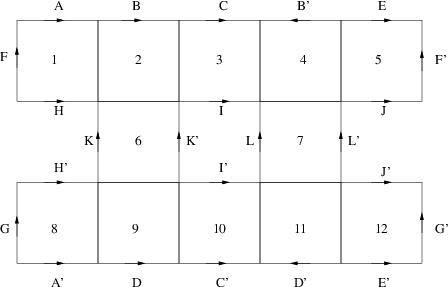
Note however, that if the origami is non-oriented, there is a canonical double covering (ramified precisely over the points, where $2$ squares abutt), which is an oriented origami.
In the sequel we will treat only the oriented case. A neccessary and sufficient condition for an origami to be oriented is that the transition functions between the charts consist only of translations. In origami language this means that upper (resp. left) edges should be glued to lower (resp. right) edges preserving global orientation.

Note that by identifying $\mathbb{R}^{2}$ with $\mathbb{C}$ we used the elliptic curve with $j(E)=1728$ in the first definition. This choice plays no role in the sequel, because the geodesic curve generated by $(X,q)$ is independent of this choice.

The fact that origamis indeed define Teichmüller curves, follows from the result of [4], that $\overline{{\rm Stab}(\tilde{\char 17\relax})}$ is commensurable with ${\rm PSL}_{2}(\mathbb{Z})$. This will also follow from the Hurwitz space description in section 3.

The quadratic differential $q$ on $X$ is obtained using the origami covering as $q=\omega^{2}$, where $\omega=\pi^{*}\omega_{E}$ and $\omega_{E}$ is the unique (up to scalar multiple) holomorphic differential on $E$.

In the case of origamis it is natural to consider the groups ${\rm Stab}(\tilde{\char 17\relax},[n])$ (or ${\rm Stab}(\tilde{\char 17\relax},n)$), where the marked $n$ points are the preimages $\pi^{-1}(\infty)$. This is for two reasons: First, this finite set of additional marked points replaces ${\rm Stab}(\tilde{\char 17\relax})$ by a subgroup of finite index (see [4]). Note that not any set of additional marked points has this property, see [3]. Second, the following definitions are best suited with the Hurwitz space interpretation in section 3 and yield that $\overline{{\rm Stab}(\tilde{\char 17\relax})}$ is contained in ${\rm PSL}_{2}(\mathbb{Z})$.

The map $\mathbb{H}/{\rm PSL}(X,q)\to M_{g}$ is generically injective and actually injective up to finitely many normal crossings, because it is the image of a geodesic locus under the quotient map of a discrete group. But the map $C\to M_{g}$ might be (see the following example) a composition of a covering and a generically injective map. If we want to reestablish injectivity, we will consider the origami curve in $M_{g,[n]}$, the moduli space of curves with $n$ non-ordered points.
To give an example that $\Gamma(\pi)$ is a proper subgroup of $\overline{{\rm Stab}(\tilde{\char 17\relax})}$ consider the following thick $L$ (see figure $2$: The sides $L_{i}$ are glued with $R_{i}$ and $D_{i}$ with $U_{i}$, preserving the global orientation. One checks that for this origami the matrix $\left(\begin{array}[]{cc}0&-1/2\\ 2&0\\ \end{array}\right)$ is in ${\rm PSL}(X,q)$ but neither in $\Gamma(\pi)$ nor in ${\rm PSL}_{2}(\mathbb{Z})$.

In this language the affine group $\Gamma(\pi)$ is the image under $D$ of the subgroup of ${\rm Aut}^{+}(\pi_{1}(E^{*}))$ that fixes $\pi_{1}(X)$ (as set).

With this description the following Lemma is obvious:

Origami curves were defined in the previous sections as quotients $C=\mathbb{H}/\Gamma(\pi)$ of discs in Teichmüller space, hence in the analytic category. But the differential $\omega$ (or $q=\omega^{2}$) was defined by covering data of an elliptic curve (e.g. $E_{1728}$). One expects that the (orbifold) origami curve in the analytification of a component of an algebraic Hurwitz (stack resp.) space. We prove here that this is indeed the case.

We start with generalities on (algebraic) Hurwitz stacks. Roughly speaking they parametrize isomorphism classes of coverings. Isomorphism here means isomorphism over a fixed base curve. Notations in this section follow Wewers ([23]). We only need covers of smooth schemes and we assume all schemes to be schemes over $\mathbb{Q}$.

Let $f:{\mathcal{E}}\to{\mathcal{M}}$ denote the universal family of curves over the smooth stack ${\mathcal{M}}$. Fix a (”ramification”) divisor ${\mathcal{D}}/{\mathcal{M}}$. Of course we have elliptic curves, maybe with additional structures in mind.
For any ${\mathcal{M}}$-scheme $S$ let ${\mathcal{H}}_{\mathcal{E}}(S)$ be the category of finite covers $X\to E_{S}$ of fixed degree $d$ and fixed genus $g$ of $X$, ramified over $D_{S}:={\mathcal{D}}\times_{\mathcal{M}}S$, where $E_{S}:={\mathcal{E}}\times_{\mathcal{M}}S$. (Maybe the notation ${\mathcal{H}}_{{\mathcal{E}},g,d}$ would be more precise.) A morphism from $X\to E_{S}\to S$ to $X^{\prime}\to E_{S^{\prime}}\to S^{\prime}$ is a morphism $S\to S^{\prime}$ plus a morphims $X\to X^{\prime}$ over the induced morphism $E_{S}\to E_{S^{\prime}}$. We cite Th. 4.1.2 from [23]:

If we replace in the above definition ${\mathcal{M}}$ by ${\mathcal{M}}_{\mathbb{C}}^{\rm an}$ we obtain an analytic stack ${\mathcal{H}}_{\mathcal{E}}^{\rm an}$, whose coarse moduli space is $(H_{\mathcal{E}})_{\mathbb{C}}^{\rm an}$. In the sequel we do not distinguish between ${\mathcal{E}}$ and ${\mathcal{E}}_{\mathbb{C}}$ for simplicity of notation.

Proof: Consider the analytic stack ${\mathcal{T}H}_{\mathcal{E}}$ whose objects (over $S$) are coverings $X\to E_{S}\to S$ in $({\mathcal{H}}_{\mathcal{E}})_{\mathbb{C}}^{\rm an}(S)$ with compatible Teichmüller markings on $X$ and $E_{S}$. Because ${\mathcal{T}}_{g}$ is étale over $({\mathcal{M}}_{g})^{\rm an}_{\mathbb{C}}$ and because of Prop. 3.1 the functor ’forget $X$’ exhibits $({\mathcal{T}H}_{\mathcal{E}})$ as an étale cover of ${\mathcal{T}}_{1,1}\cong\mathbb{H}$. Hence it consists of several disjoint copies of $\mathbb{H}$, one of which contains $\pi:X\to E$. We call this connected component ${\mathcal{T}H}_{\pi}$ and we let $({\mathcal{H}}_{\pi})^{\rm an}_{\mathbb{C}}$ be the corresponding component of $({\mathcal{H}}_{\mathcal{E}})_{\mathbb{C}}^{\rm an}$ (after forgetting the Teichmüller marking). $({\mathcal{H}}_{\pi})^{\rm an}_{\mathbb{C}}$ stems from a uniquely determined connected component ${\mathcal{H}}_{\pi}$ of ${\mathcal{H}}_{\mathcal{E}}$.

It remains to check that $({\mathcal{H}}_{\pi})^{\rm an}_{\mathbb{C}}$ is the quotient stack ${\mathcal{T}H}_{\pi}/{\rm Stab}(\tilde{\char 17\relax},[n])$. This easily follows from unwinding definitions, noting that Deck transformations respect the set $\pi^{-1}(\infty)$. $\Box$

Proof: For the second claim note that the forgetful functor ${\mathcal{H}}_{\mathcal{E}}\to{{\mathcal{M}}_{g}}$ is defined over $\mathbb{Q}$. Hence the morphism between the geometric components of the (coarsely) representing schemes are defined over finite extensions of $\mathbb{Q}$. $\Box$.

In this section we examine two origamis, the smallest origami which is not an elliptic curve and the smallest one that can be used for $\widehat{GT}$-considerations. In both cases we explicitely describe the equation of the geodesic curve.

Fix $\sigma\in G_{\mathbb{Q}}$ and let $K={\rm Fix}(\sigma)$ its fixed field. We first prove faithfulness in a weak sense:

Proof: We will derive this from a corresponding result concerning dessins d’enfants:
As shown in [21] Th. II.4 there exists a Belyi morphism $\beta:\mathbb{P}_{\overline{\mathbb{Q}}}^{1}\to\mathbb{P}_{\overline{\mathbb{Q}}}^{1}$, i.e. unramified outside $\{0,1,\infty\}$, such that ${}^{\sigma}\beta\not\cong\beta$. We may also suppose that $\beta$ is pure, i.e. that precisely the preimage of $1$ consists only of points ramified of order $2$.
Let $h:E\to\mathbb{P}^{1}$ be the double cover ramified over $\{0,1,\lambda,\infty\}$. We take the pullback of $\beta$ by the morphism $h$ and call the desingularisation $\widetilde{\pi}:X\to E$. The morphism $\widetilde{\pi}$ is ramified at most over $\{0,1,\lambda,\infty\}$ and hence after multiplication by $2$ the map $\pi=[2]\circ\widetilde{\pi}$ defines an origami.
Suppose there is a $\overline{\mathbb{Q}}$-isomorphism $\varphi:X\to\,^{\sigma}\!X$ with $\pi=\,^{\sigma}\pi\circ\varphi$. We claim that this implies $\widetilde{\pi}=\,^{\sigma}\widetilde{\pi}\circ\varphi$: As $E$ and $[2]$ are defined over $K$ the difference morphism $\widetilde{\pi}-\,^{\sigma}\widetilde{\pi}\circ\varphi$ maps to the finite kernel of $[2]$. We can conclude because $\beta^{-1}(1)$ and hence $(\widetilde{\pi})^{-1}(h^{-1}(1))$ is distinguished by the purity hypothesis.
Let $\tau$ be the involution on $X$ induced by the elliptic involution of $E$. Once we have shown that $\varphi\circ\tau=\,^{\sigma}\!\tau\circ\varphi$, the isomorphism $\varphi$ descends to $\mathbb{P}^{1}$ and gives the desired contradiction. But both $\tau$ and $\varphi^{-1}\circ\,^{\sigma}\!\tau\circ\varphi$ are involutions with the same number of fixed points. Since $X/\langle\tau\rangle$ the involutions have to coincide by the uniqueness of the hyperelliptic involution. $\Box$

Looking closer at the proof of Th. II.4 in [21], we can choose the morphism $\beta$ in the above proof such that its ramification over $1$ consists only of points of order $2$, that $\beta$ is totally ramified over $\infty$ and that the ramification behaviour over $0$ is different from these two. Let ${\mathcal{M}}_{1,1}^{[2]}$ denote the moduli stack of elliptic curves with level $2$ structure. We will use the non-calligraphic letters (e.g. $M_{1,1,}^{[2]}\cong\mathbb{P}^{\ast}$) for the corresponding coarse moduli spaces.

Proof: We continue with the construction and the notations from the proof of the above lemma. First we prove that ${\mathcal{M}}_{1,1}^{[2]}$ surjects onto $C^{\rm orb}(\pi)$:
For this purpose we need to construct a family over ${\mathcal{M}}_{1,1}^{[2]}$ of coverings of the universal family ${\mathcal{E}}\to{\mathcal{M}}_{1,1}^{[2]}$. Let $h:{\mathcal{E}}\to\mathbb{P}^{1}$ be the quotient by the elliptic involution $h_{E}$ followed by the canonical projection $\mathbb{P}^{1}\times{\mathcal{M}}_{1,1}^{[2]}\to\mathbb{P}^{1}$. (The quotient ${\mathcal{E}}/h_{E}$ is indeed a trivial bundle as it contains $4$ disjoint (Weierstraß) sections). Take the desingularisation of $\mathbb{P}^{1}\times_{\mathbb{P}^{1}}{\mathcal{E}}\to{\mathcal{M}}_{1,1}^{[2]}$, where the morphisms in the fibred product are $\beta$ and $h$ respectively. The singular locus of the fibre product is étale over the base and thus the desingularisation is still a flat family of curves, which we denote by ${\mathcal{X}}\to{\mathcal{M}}_{1,1}^{[2]}$. Let $\pi:{\mathcal{X}}\to{\mathcal{E}}$ denote the composition of the second projection with the multiplication by $2$. We thus constructed a topologically locally trivial family of coverings over ${\mathcal{M}}_{1,1}^{[2]}$. This family contains by construction the covering $X\to E$ of the preceding lemma (which we also denoted by $\pi$), hence does the job by Prop. 3.2.

It remains to exclude that ${\mathcal{M}}_{1,1}^{[2]}\to C^{{\rm orb}}$ is a cover of degree greater than one or equivalently that $\mathbb{P}^{*}\to C(\pi)$ is a cover of degree greater than one. We have to exclude that the affine group of $\pi$ is bigger than $\Gamma(2)$.
Fix a fibre $X\to E^{[2]}\to E$ of $\pi:{\mathcal{X}}\to{\mathcal{E}}$ and call this covering also $\pi=[2]\circ\tilde{\pi}$. The subgroup of $\pi_{1}(E^{\ast})=\langle x,y\rangle$ corresponding to $[2]$ is generated by $x^{2},y^{2},xy^{2}x$ and $yx^{2}y$. It is obviously characteristic and hence by Lemma 2.6 an affine diffeomorphism $\varphi:X\to X$ over $\overline{\varphi}:E\to E$ descends to an affine diffeomorphism $\varphi^{[2]}:E^{[2]}\to E^{[2]}$. If $D(\overline{\varphi})$ is not in $\Gamma(2)$, the morphism $\varphi^{[2]}$ has to permute the $2$-division points of $E^{[2]}$.
But the fibres of $\tilde{\pi}$ over the $2$-division points are different by our hypothesis on $\beta$: One fibre consists of unramified points that are all fixed by the hyperelliptic involution of $X$. One consists of unramified points that are pairwise interchanged by the hyperelliptic involution. One consists of $2$ points and the last one has a ramification behaviour different from the above.
As an affine diffeomorphism has to preserve the ramification order and fixed points of the hyperelliptic involution, this leads to a contradiction. $\Box$

As usual let $d=\deg(\pi)$. We need one more topological lemma. For the notation compare with the Remarks 2.7 and 2.8.

Proof: Consider $h:E^{[2]}\to\mathbb{P}^{1}$ as unramified covering over the $4$-punctured $\mathbb{P}^{1}$. Denote the loops around $0,1,\lambda,\infty\in\mathbb{P}^{1}$ by $x_{0},x_{1},x_{2},x_{3}$ such that $x_{3}x_{2}x_{1}x_{0}=1$. Choose loops around the Weierstraß points on $E^{[2]}$ denoted by $c_{0},\ldots,c_{3}$ and $a,b\in\pi_{1}((E^{[2]})^{*})$ such that $[a,b]c_{3}c_{2}c_{1}c_{0}=1$. This numbering is consistent with supposing that

The isogeny $[2]$ doubles the number of unit height cylinders in each direction. As $\tilde{\pi}$ is totally ramified over $h^{-1}(\infty)$ all the maximal cylinders of $\pi$ in each direction have height $2$. What we need to ensure is hence that the monodromy images $m(a),m(ab),m(b)\in S_{d/4}$ corresponding to $\tilde{\pi}$ consist of $1$ (resp. $d/8$, resp. $r\not\in\{1,d/8\}$) cycles.
By construction of $\tilde{\pi}$ as fibre product the monodromy $m(c)$ for $\tilde{\pi}$, where $c\in\pi_{1}((E^{[2]})^{\ast})$ coincides with the monodromy of $h_{*}(c)$ for $\beta$.
Since the monodromy of $x_{2}$ is trivial, the number of cycles of $m(a)$ equals the number of preimages $\beta^{-1}(1)$, which was $d/8$. The number of cycles of $m(b)$ equals the number of preimages $\beta^{-1}(\infty)$, which was one. Finally, the number of cycles of $m(ab)$ equals the number $r$ of preimages of $0$.
Going back to the construction of $\beta$, we show that we may choose $r\not\in\{1,d/8\}$. Suppose $\beta_{0}$ is a Belyi morphism as constructed in [21], totally ramified over $\infty$. If the number of preimages of $0$ and $1$ does not sum up to $\deg(\beta)/2$, we take $\beta=4\beta_{0}(1-\beta_{0})$. Otherwise we take $\beta_{1}=x^{2}\circ\beta_{0}$ to ensure this condition and then take $\beta=4\beta_{1}(1-\beta_{1})$. $\Box$

Proof: Take $C$ as constructed in the preceding lemmas and assume that $j(C)=j^{\sigma}(C)$. We claim that this is equivalent to $j$ being is defined over $K$. To prove this, it is equivalent to show that

using descent for morphisms between varieties defined over $K$. The assumption implies that there exists an automorphism $\varphi$ of $j(C)$, such that

By Lemma 5.3 and Remark 2.8 the stable curves corresponding to the cusps of $C$ have pairwise distint number of nodes. This implies that $j(C)\cong\mathbb{P}^{\ast}$. Furthermore the number of nodes of a singular fibre is $G_{\mathbb{Q}}$-invariant. Hence $\varphi$ has to be the identity and this proves the claim.

Take a $K$-rational point $x$ of $C$ and denote the corresponding curve by $X$. The above claim implies the existence of an isomorphism $\sigma_{X}:X\to X^{\sigma}$. By construction we still have the morphisms $\pi:X\to E$ and $\pi^{\sigma}:X^{\sigma}\to E^{\sigma}$ plus the canonical morphism $\sigma_{E}:E\to E^{\sigma}$. If we knew that $\pi^{\sigma}\circ\sigma_{X}=\sigma_{E}\circ\pi$ then Lemma 5.1 would lead to a contradiction.

On $X$ (resp. $X^{\sigma}$) we have the differentials $\omega_{X}=\pi^{*}\omega_{E}$ (resp. $\omega_{X^{\sigma}}=\pi^{*}\omega_{E^{\sigma}}$). Our second claim is that $\omega_{X}=\sigma_{X}^{*}\omega_{X^{\sigma}}$ (up to a multiplicative constant).
The map $\sigma_{M_{g}}$ not only maps $[X]\in(M_{g})_{\overline{\mathbb{Q}}}$ to $[X^{\sigma}]\in({\mathcal{M}}_{g})_{\overline{\mathbb{Q}}}^{\sigma}$ but also $C$ to $C^{\sigma}$. Hence the tangent vector $t_{X}$ at $[X]$ to $C$ is mapped to the tangent vector $t_{X^{\sigma}}$ at $[X^{\sigma}]$ to $C^{\sigma}$. Now tensor the whole situation by $\mathbb{C}$ for some fixed embedding $\overline{\mathbb{Q}}\to\mathbb{C}$. The Teichmüller metric induces a (non-linear, but functorial) duality between the projectivised tangent and cotangent space of to $M_{g}$ at $X$. By construction $(\omega_{X})^{2}$ is the unique (up to scalar multiple) quadratic differential corresponding to $t_{X}$ via this duality. The same is true for $X^{\sigma}$, $t_{X^{\sigma}}$ and $(\omega_{X^{\sigma}})^{2}$. This implies that $w_{X}^{2}=(\sigma_{X}^{*}\omega_{X^{\sigma}})^{2}$ and establishes the second claim.

References

- [1] Gildenhuys, D., Lim, C.-K. Free pro--groups, Math. Z. 125 (1972), 233–254
- [2] Lochak, P., Schneps, L. (eds), Geometric Galois actions, Vol I and II, London Math. Soc. LN Series, 242 and 243 (1997)
- [3] Gutkin, E., Hubert, P., Schmidt, T., Affine diffeomorphisms of translation surfaces: Periodic points, Fuchsian groups and arithmeticity, Ann. Sci. Ecole Norm. Sup. 4e ser., t. 36 (2003), 847–866
- [4] Gutkin, E., Judge, C., Affine mappings of translation surfaces, Duke Math. J. 103 No. 2 (2000), 191–212
- [5] Hatcher, A., Lochak, P., Schneps, L., On the Teichmüller tower of mapping class groups, J. reine ang. Math. 521 (2000), 829–860
- [6] Hubert, P., Schmidt, T.A., Invariants of translation surfaces, Ann. Inst. Fourier, Grenoble, 51 No. 2 (2001), 461–495
- [7] Ichikawa, H., Teichmüller groupoids and Galois action, J. reine angew. Math. 559 (2003), 95–114
- [8] Ihara, Y., Nakamura, H., On deformation of maximally degenerate stable marked curves and Oda’s problem, J. reine angew. Math. 487 (1997), 125–151
- [9] Kani, E., Hurwitz spaces of genus covers of an elliptic curves, Collect. Math. 54, No. 1 (2003), 1–51
- [10] Kontsevich, M., Zorich, A., Connected Components of the Moduli Space of Abelian Differentials with Prescribed Singularities, Invent. Math. 153 (2003), 631–678
- [11] Lochak, P., On arithmetic curves in the moduli space of curves, preprint (2003)
- [12] Lochak, P., Nakamura, H., Schneps, L., Eigenloci of 5 point configurations on the Riemann Sphere and the Grothendieck-Teichmüller group, preprint (2003)
- [13] Masur, H., On a class of geodesics in Teichmüller space, Ann. of Math. 102 (1975), 205–221
- [14] McMullen, C., Billiards and Teichmüller curves on Hilbert modular suraces, Journal of the Amer. Math. Soc. 16 No. 4 (2003), 856–885
- [15] Nakamura, H., Galois representations in the profinite Teichmüller modular groups, in [2] Vol. I, 159–173
- [16] Nakamura, H., Limits of Galois Representations in Fundamental Groups Along Maximal Degeneration of Marked Curves, II, Proc. of Symp. Pure Math. 70 (2002), 43–78
- [17] Nakamura, H., Schneps, L. On a subgroup of the Grothendieck-Teichmüller group acting on the tower of profinite Teichmüller modular groups, Inv. Math. 141 (2000), 503–560
- [18] Nakamura, H., Tsunogai, H., Harmonic and equianharmonic equations in the Grothendieck-Teichmüller group, Forum Math. 15 (2003), 877–892
- [19] Ribes, L., Zalesskii, P., Profinite groups, Erg. der Math. und ihrer Grenzgeb. 40, Springer (2000)
- [20] Schmithüsen, G., An Algorithm for Finding the Veech Group of an Origami, preprint (2003)
- [21] Schneps, L., Dessins d’enfants in: The Grothendieck Theory of Dessins d’enfants, LMS Lecture Notes 200 (1994)
- [22] Schneps, L., Automorphisms of curves and their role in Grothendieck-Teichmüller theory, preprint (2004)
- [23] Wewers, S., Constructing Hurwitz spaces, Dissertation, Essen (1998)
Martin Möller: Universität Essen, FB 6 (Mathematik)
45117 Essen, Germany
e-mail: martin.moeller@uni-essen.de