Entropy-minimising models of surface diffeomorphisms relative to homoclinic and heteroclinic orbits
Abstract
In the theory of surface diffeomorphisms relative to homoclinic and heteroclinic orbits, it is possible to compute a one-dimensional representative map for any irreducible isotopy class. The topological entropy of this graph representative is equal to the growth rate of the number of essential Nielsen classes of a given period, and hence is a lower bound for the topological entropy of the diffeomorphism. In this paper, we show that this entropy bound is the infemum of the topological entropies of diffeomorphisms in the isotopy class, and give necessary and sufficient conditions for the infemal entropy to be a minimum.
Mathematics subject classification: Primary: 37E30. Secondary: 37B10, 37C27, 37E25.
1 Introduction
In the Nielsen-Thurston theory of surface diffeomorphisms [CB88], it is possible to find a diffeomorphism in each isotopy class which minimises both the number of periodic orbits of each period, and the topological entropy [Han85, Fat90, Jia96, Boy99]. A constructive proof can be given [BH95, FM93]; a one-dimensional representative of the diffeomorphism called a train track is computed and the Thurston-minimal model is easily constructed from this.
The case of diffeomorphisms relative to homoclinic orbits to a saddle point is more complicated. It is well-known that any diffeomorphism with a transverse homoclinic point has positive topological entropy, but it is easy to construct examples of such diffeomorphisms with arbitrarily small entropy. Therefore, it may not even be possible to find a diffeomorphism realising the lower bound of the entropy.
In this paper, we discuss the relation between the Nielsen entropy [Jia83], which measures the growth rate of the number of essential Nielsen classes of periodic points, and the infemal entropy in the isotopy class. The Nielsen entropy is equal to the topological entropy of the graph representative, which can be computed using the algorithms described in [Col02, Col]. The key step is to represent the isotopy class relative to the homoclinic/heteroclinic orbits using a trellis, which is a subset of the homoclinic tangle of the saddle periodic points. We show that under mild non-degeneracy conditions, the Nielsen entropy is equal to the infemum of the topological entropies in the isotopy class. This result can be considered an optimality result for the computational techniques of the trellis theory.
The proof that the Nielsen entropy is infemal involves the construction of uniformly-hyperbolic diffeomorphisms realising the entropy bound arbitrarily closely. In certain cases, it is possible to construct a uniformly-hyperbolic diffeomorphism realising the entropy bound. We show that the only obstruction to the construction of a uniformly hyperbolic diffeomorphisms realising the entropy bound is the existence of almost wandering segments; intervals of (un)stable manifold which must contain intersection points under some iterate of any representative diffeomorphism, but for which no bound on the number of iterates exists. Hence the Nielsen entropy is a minimum if and only if there are no almost wandering segments. Under these conditions, we also show that if the system irreducible, then any isotopy which removes any of the intersection points of the trellis also reduces the Nielsen entropy.
The conditions on the existence of entropy minimisers is delicate, and relies on the class of system under consideration. We only consider the problem in the case of homoclinic orbits to a saddle point in which the local stable and unstable branches are known, such as a hyperbolic saddle periodic orbit of a diffeomorphism which are the typical case in applications. If we instead consider systems for which we allow periodic points modelled on -prong singularities, then it is immediate that there are no almost wandering segments, and it is always possible to introduce extra branches ending in attracting or repelling periodic orbits and hence construct a homeomorphism realising the entropy bound. A similar situation occurs if we only require that the stable and unstable curves of the trellis are, respectively, positively and negatively invariant.
2 Trellises, curves and graphs
We introduce the notion of trellis and trellis type, and relate these to the well-known notion of homoclinic/heteroclinic orbit and tangle. We give a number of definitions which allow us to describe some of the basic properties of trellises. We then give some definitions concerning homotopy and isotopy classes of curves. Finally, we review the definitions of (thick) graphs, and show how to associate a graph representative to each irreducible trellis type.
2.1 Tangles and Trellises
A tangle is the figure formed by the stable and unstable manifolds of a collection of periodic saddle orbits of a surface diffeomorphism . We denote the stable and unstable sets of by and respectively. If consists of a single point, then is a homoclinic tangle, otherwise is a heteroclinic tangle.
Definition 2.1 (Trellis)
Let be a diffeomorphism of a surface with a finite invariant set of hyperbolic saddle points. A trellis for is a pair , where and be subsets of and respectively such that:
- 1.
and both consist of finitely many compact intervals with non-empty interiors,
- 2.
and .
We denote the set of periodic points of by , and the set of intersections of and by .
We write to denote the pair consisting of a diffeomorphism and a trellis for . We use the notation in statements which hold for both stable and unstable manifolds. If the diffeomorphism under consideration is clear from the context, we abbreviate to , and if the periodic point set is also clear, we simply write . If is a point of , then the stable and unstable curves passing through are denoted and respectively. We denote the closed interval in with endpoints and by and the closed interval by .
An intersection point of a tangle is a a point in , and is a point of a homoclinic or heteroclinic orbit. An intersection point is a primary intersection point or pip if and are disjoint. An intersection point is transverse or tangential according to whether and cross transversely or tangentially at An end intersection of a trellis is an intersection which does not lie in two segments of (so lies in at least one end of ).
An arc of is a closed subinterval of with endpoints in . A segment of is an arc of with no topologically transverse intersection points in its interior. An end interval of a trellis is a subintervals of which does not lie in any segment.
A branch of a trellis is a set of the form A branch is trivial if it does not intersect any other branch. Note that points and lie in the same branch of if and only if and lie in the same component of for some . Note that a branch need not be connected.
An open region of is a component of . A (closed) region is the closure of an open region, and hence includes the stable and unstable boundary segments. A (closed) domain of is an closed subset of with boundary in ; note that we do not require domains to be simply-connected, though this is the case we will usually consider. We will denote domains by the letter , and regions by the letter . Note that we do not require domains or regions to be simply-connected. There are two special types of region which play an important role, namely bigons and rectangles. A bigon is a region which is a topological disc bounded by one stable and one unstable segment with internal angles less than . A rectangle is a region which is a topological disc bounded by two stable and two unstable segments with internal angles less than . Bigons play a similar role in the trellis theory as do critical points in the kneading theory, and may be called critical regions; rectangles can be foliated by stable and unstable leaves, and may be called regular regions.
In general, we do not have much control over the geometry of a trellis. The exception is near a point of , where the dynamics are conjugate to a linear map. It is important to consider how the nontrivial branches divide the surface in a neighbourhood of .
Definition 2.2 (Quadrant, secant and coquadrant)
Let be a trellis, and be the nontrivial branches of , and be a point of . Then a sector of at is a local component of a region of in a neighbourhood of . A sector is a quadrant if it intersects no trivial branches, in which case the boundary includes a single unstable branch and a single stable branch with internal angle less than . A sector is an secant if it intersects a single trivial branch; if this is a branch of the secant is attracting, and if this is a branch of , the secant is repelling. A sector is a coquadrant if it intersects two trivial branches, and so the nontrivial branches and subtend an angle greater than in .

Quadrants, secants and coquadrants are shown in Figure 1. The region containing a quadrant is denoted . The image of a quadrant is the quadrant containing ; note that is the same branch as . A stable segment with endpoint intersects lies on the -side of if locally lies on the same side of at as does at . Similarly, an unstable segment with endpoint intersects lies on the -side of if locally lies on the same side of at as does at . The segment in Figure 1(a) lies on the -side of .
By an isotopy relative to , we mean an isotopy such that is a tangle for for all . We say and are conjugate if there is a homeomorphism such that and . These relations allow us to define the equivalence classes of trellis map which will be our primary object of study.
Definition 2.3 (Trellis mapping class and trellis type)
The trellis mapping class is the set of all pairs for which is isotopic to relative to . The trellis type is the set of all pairs which are conjugate to a map isotopic to relative to . We consider and equivalent if .
A trellis type is an iterate of the trellis type if and is an -iterate of .
A surface diffeomorphism with a periodic saddle orbit has infinitely many trellises, which are partially ordered by inclusion. Taking a smaller trellis gives a subtrellis, and a larger trellis a supertrellis. Then is a subtrellis of if , and is a subtrellis of if . We say is a supertrellis of and is a supertangle of . Similarly, the trellis type is a subtrellis of . Of particular importance are those supertrellises which can be obtained by iterating segments or branches. A trellis is an -iterate of if there exist positive integers and such that and . A trellis is an -extension of if there exists such that
An iterate/extension is a stable iterate/extension if and an unstable iterate/extension if .
The main difference between extensions and supertrellises is that for an extension, but may be a strict subset of for a supertrellis. This difference makes the analysis of supertrellises slightly more complicated than that of extensions.
If is a segment of and is not a subset of , we can take a stable -extension with . We say this extension is formed by taking a backward iterate of . In a similar way, we can form extensions by taking backward iterates of arcs of , or forward iterates of arcs of . For these extensions, the endpoints of any curve of lie in the set .
We say a supertrellis is a minimal supertrellis of if has minimal number of intersections among all supertrellises with endpoints in the same segment. An equivalent formulation of a minimal supertrellis is that every bigon contains a point of the set . A minimal supertrellis which is an extension or iterate is, respectively, a minimal extension or a minimal iterate.
The most important dynamical feature of a trellis type is its entropy.
Definition 2.4 (Entropy)
The entropy of a trellis type , denoted is the infemum of the topological entropies of diffeomorphisms in ; that is
If this infemum is not a minimum, we sometimes write .
Example 2.5 (The type- trellis)

The type- trellis is depicted in Figure 2. It is formed by subsets of the stable and unstable manifolds of the direct saddle fixed point (i.e. the saddle point with positive eigenvalues) of the Hénon map for certain parameter values. The stable and unstable sets are subsets of the stable and unstable manifolds of the saddle fixed point . The branches of this trellis are connected and the all intersection points are transverse. The points , , and are primary intersection points on a single homoclinic orbit. The orbits of the intersection points and are shown in white dots. These orbits are called forcing orbits for the type- trellis; it is essentially impossible to remove any intersection points of the trellis by an isotopy without first removing and in a homoclinic bifurcation. Throughout this paper we follow the convention of showing forcing orbits as which dots, and primary intersection points as crosses.
There are ten regions, an unbounded region , five bigons, three rectangles and a hexagon. The quadrant is contained in the region . Under the Smale horseshoe map, there is a Cantor set of nonwandering points contained in the (closed) regions and , including a fixed point in . All other points are wandering except for an attracting fixed point at the end of one unstable branch of in . The topological entropy of the Smale horseshoe map is , where is the largest root of the polynomial . Any diffeomorphism with this trellis type must have topological entropy .
Notice that one of the unstable branches of the trellis ends in an attracting fixed point, and one of the stable branches is non-existent. Both of these are therefore trivial branches.
Given a diffeomorphism with a trellis , we can obtain a canonical map of pairs by cutting along , as described in [Col99]. The topological pair obtained by cutting along the unstable curve is denoted . The diffeomorphism lifts for a map on . Notice that the pair contains the pair as an open subset which is invariant under . Indeed, can be regarded as a natural compactification of , and the homotopy properties of and are essentially the same. In order that the stable set be well-behaved after cutting, we only consider proper trellises, for which and . In other words, a trellis is proper if the endpoints of intervals in lie in , but the endpoints of intervals in do not lie in .
Definition 2.6 (Well-formed trellises)
We say a proper trellis for a diffeomorphism is well-formed if every component of contains a point of .
Restricting to well-formed trellises will be important when considering the graph representative defined in Section 2.4, as it gives a necessary condition for the topological entropy of the graph representative to be an optimal entropy bound for the trellis mapping class.
2.2 Attracting and repelling regions
As well as saddle periodic orbits, codimension-zero sets of diffeomorphisms also have attracting and repelling periodic orbits. Clearly, a stable segment cannot be in the basin of attraction of an attracting orbit, and neither can an unstable segment be in the basin of a repelling orbit. However, it is possible for the interior of an entire region to lie in the basin of an attracting or repelling periodic orbit. Such regions are called stable or unstable regions.
Definition 2.7 (Stable and unstable regions)
Let be a trellis mapping class. A domain of is stable if there is a diffeomorphism in and a periodic orbit of such that as for all in the interior of . If contains a point of , then is attracting. Similarly, a domain is unstable if there is a diffeomorphism in and a periodic orbit of such that as for all in the interior of , and if contains a point of , then is repelling.

Two examples of attracting domains are shown in Figure 3. All points in the shaded domains are in the basin of attraction of the stable periodic point. Note that is disjoint from the interior of . Repelling domains are similar. Stable and unstable domains are wandering sets, unless they contain the attracting or repelling periodic orbit.

A region which contains an attractor and a repellor is called unbounded region, by analogy with the unbounded region of the planar Smale horseshoe, for which the repellor is the point at infinity. Figure 4 shows an unbounded region near a fixed point . All points in lie in the basin of attraction of an attracting fixed point , and all points in lie in the basin of a repelling fixed point . Since and cover the interior of , all points in the interior of are wandering, apart from and .
Definition 2.8 (Chaotic region)
Let be a trellis mapping class. A region is chaotic if for every diffeomorphism in , there exists an integer such that contains a point in the interior of .
We shall see that a chaotic region supports entropy, in the sense that for any diffeomorphism , there is an ergodic measure with positive entropy such that .
An open segment which is in the basin of a repelling periodic orbit is also a wandering set, as is an open segment which is in the basin of an attracting periodic orbit. There are some nonwandering segments such that any finite iterate need not contain an intersection point. We call such segments almost wandering.
Definition 2.9 (Almost wandering segment)
Let be a trellis mapping class. An open segment is almost wandering if it is nonwandering, but for any integer there exists a diffeomorphism the iterate of the segment by contains no intersection points.
Hence an open stable segment is almost wandering if for any positive integer , there exists such that , but for any diffeomorphism , there exists such that . A similar statement holds for unstable segments.
2.3 Curves and homotopies
Our main tool for studying the geometry, topology and dynamics associated with trellis maps will be to consider curves embedded in pairs , which we will usually take to be either the cut surface of the graph . Since the topological pair is obvious from the trellis, we will usually draw curves in as curves embedded in the original surface , and, wherever possible, ensure these curves are disjoint from .
Our curves will be maps in this category of topological pairs, . The path of such a curve is the set . For the most part, we are only interested in curves up to homotopy or isotopy, and we always take homotopies and isotopies of curves through maps of pairs. For Nielsen theory we will always keep the endpoints fixed during the homotopy. For most other purposes, we only consider curves for which , so the endpoints lie in , but may move. If is a curve and contains we say has endpoints in ; if equals we say has endpoints only in .
Reparameterising a curve does not change its path, but may change the set which maps into . This means that different parameterisations of the same path may not even be comparable under homotopy. However, we consider different parameterisations of the same curve as equivalent.
Definition 2.10 (Equivalence of curves)
Curves and are equivalent if there is a homeomorphism with such that as curves . The homotopy may be taken relative to endpoints, as appropriate.
We can also define a partial order on curves in a similar way:
Definition 2.11 (Tightening curves)
Let and be exact curves. We say tightens to if there is an injective map such that as curves .
If tightens to , then can be thought of as more complicated than . It is clear that the tightening relation is a partial order on homotopy classes of curves. We are especially interested in iterates with minimal number of components intersecting .
Definition 2.12 (Minimal iterate)
Let and be a simple curve with endpoints in . Then a minimal iterate of under is a curve which is homotopic to relative to and which minimises the number of components of intersections with . We let , and consider as a curve . If we further require that in intersection is isolated whenever possible, then the curve is well-defined up to equivalence, so we obtain a well-defined map on equivalence classes of curves given by .
Note that by we mean , and not , which typically has fewer intersections.
2.4 Graph maps
Our main tool for computing and describing the dynamics forced by a trellis mapping class or trellis type is to relate the trellis map to a graph map. We will mostly use the same terminology and notation for graphs as in [BH95], though our terminology for thick graphs is closer to that of [FM93].
In particular, a graph is a one-dimensional CW-complex with vertices and edges . The reverse of an edge is denoted . An edge-path is a list of oriented edges of such that for , and an edge loop is a cyclically-ordered list of edges. The trivial edge-path contains no edges and is denoted . An edge-path back-tracks if for some , otherwise it is tight. A graph map is a self-map of taking a vertex to a vertex, and edge to an edge-path such that for all directed edges . The derivative map takes oriented edges to oriented edges or , with if and if .
We will always consider a graph embedded in a surface by an embedding . This induces a natural cyclic order on the oriented edges starting at each vertex. A pair of edges is a turn in at at vertex if and , so immediately follows in the cyclic order at . An edge-loop is peripheral in if is a turn in for all .
A graph embedded in a surface can be “thickened” to obtain a fibred surface or a thick graph with thick vertices and thick edges, the latter fibred by stable and unstable leaves. The inverse of this thickening is achieved by collapsing thick vertices to points, and thick edges to edges. A thick graph map is a injective map of a thick graph which is a strict contraction on the set of thick vertices, and maps thick edges so as to preserve the stable leaves. A graph map is embeddable if it can be obtained from a thick graph map by collapsing the stable leaves. The peripheral subgraph of is a maximal invariant subset of consisting of simple peripheral loops. Edges of are called peripheral edges. If for some , then is pre-peripheral. The set of pre-peripheral edges is denoted , and contains .
The transition matrix of a graph map is the matrix where counts the number of times the edge appears in the image path of edge . The largest eigenvalue of is the growth rate of , and the logarithm of the growth rate gives the topological entropy of . A length function on is a strictly-positive function . The length of an edge-path is defined to be . If is a graph map with topological entropy , then for any there is a length function with for any edge .
We relate a trellis mapping class to a graph map via the map of the topological pair obtained by cutting along the unstable curves. The result is a map of a topological pair where is a finite subset of .
Definition 2.13 (Controlled graph map)
Let be a topological pair where is a graph and is a finite subset of . The edges of containing points of are called control edges. A graph map is a controlled graph map if is a control edge whenever is a control edge.
A vertex of which is the endpoint of a control edge is called a control vertex. All other vertices are called free vertices, and edges which are not control edges are called free edges. Free edges which are neither peripheral nor pre-peripheral are called expanding edges.
A controlled graph is proper if it is connected and each free vertex has valence at least . A proper controlled graph has at most edges, and vertices, where is the number of control edges of and is the Euler characteristic of .
To relate maps of pairs on different spaces, we need the notion of exact homotopy equivalence defined in [Col01]. A graph map representing the topology of a trellis via exact homotopy equivalence is called compatible with the trellis.
Definition 2.14 (Compatible graph map)
Let be a topological pair where is a graph and is a finite subset of . Then is compatible with a transverse trellis if and are exact homotopy equivalent by an embedding . A controlled graph map of is compatible with the trellis type if the embedding is an exact homotopy equivalence between and , and and have the same orientation at points of .
Note that the inclusion induced a bijection between the regions of (and hence of ) with the regions of , and that all compatible graphs are exact homotopy equivalent. We restrict to transverse trellises since a trellis with tangencies may not have a compatible controlled graph. While it is always possible to find a topological pair which is exact homotopy equivalent to for which is a graph, it may not be possible to take to be a finite set of points.

The controlled graph shown in Figure 5 is compatible with the trellis . The control edges are shown as thick shaded lines.
There are many controlled graph maps compatible with a trellis type . To use graph maps to describe the dynamics forced by , we need to define a subclass of controlled graph maps which have minimal entropy in the exact homotopy class. These graph maps are called efficient, by analogy with Nielsen-Thurston theory. Of the efficient graph maps, there is at most one which is optimal, giving a canonical graph representative for the trellis type. Tight, efficient and optimal graph maps can be defined in terms of their actions on the turns of . In this paper, we only need the definition of an optimal graph map; other definitions can be found in [Col].
Definition 2.15 (Graph representatives)
A controlled graph map is optimal if for every turn , either , or at least one of or is a control edge. A controlled graph map is a graph representative of a transverse trellis type if is an optimal graph map which is compatible with .
The following theorem [Col] shows that every proper irreducible trellis type has a unique graph representative.
Theorem 2.16 (Existence and uniqueness of graph representatives)
Let be a proper trellis type with no invariant curve reduction. Then has a unique graph representative . Further, if and are trellis types, the graph representatives and are homeomorphic if and only if .
In particular, this result shows that the graph representative provides a convenient way of specifying a trellis type.
3 Regular domains and alpha chains
3.1 Regular domains
Any diffeomorphism is conjugate to a linear hyperbolic diffeomorphism in a neighbourhood of a point of a periodic saddle point. We therefore expect a trellis map to behave in a fairly predictable way in a neighbourhood of a point of . In particular, we know how a rectangle with sides parallel to the local stable and unstable foliations behaves. Unfortunately, for a given trellis mapping class, the neighbourhood of on which we have hyperbolic behaviour may be arbitrarily small. To deal with this problem, we introduce the concept of a regular domain, which is a rectangular domain which behaves similarly to a sufficiently small rectangular neighbourhood of a periodic saddle point.
Definition 3.1 (Regular domain)
Let be a trellis mapping pair. A rectangular domain of is a regular domain for a period- quadrant of if has sides , , and , such that
- (1u)
with ,
- (1s)
with ,
- (2u)
, and
- (2s)
.
The sides and are called adjacent sides of , and the sides and are opposite sides. The definition is given purely in terms of the topology of the trellis and the mapping of its vertices; no extensions are needed. Notice that the definition is invariant under time reversal on time reversal if we interchange and . In general, we therefore only need to prove statements on the topology of an adjacent domain for either the unstable (u) or stable (s) case.

A regular domain is shown in Figure 6. We shall always denote the vertices of a regular domain by , , and as shown. We now give a number of elementary properties of a regular domain. The first two lemmas are trivial.
Lemma 3.2
Let be a regular domain for at . Then
- 1.
If and are subsets of , then is a regular domain for at .
- 2.
If is isotopic to relative to , then is a regular domain for at .
- 3.
If is an extension of , then is a regular domain for at .
Proof.
- 1.
Since , and , the boundary of is composed of segments of . On the adjacent sides we have and . On the opposite sides, we have and similarly .
- 2.
Condition (1u) shows that , so , so condition (1u) is satisfied for . If , then , so condition (2s) is satisfied. Otherwise, for some such that contains no points of . Then since , we have , and since , we have , so condition (2s) is still satisfied. A similar argument proves conditions (1s) and (2u).
- 3.
∎
We now show how to construct regular subdomains of a regular domain.
Lemma 3.3
Let be a regular domain for at a quadrant .
- 1.
If is a curve with endpoints and , then the rectangular domain with vertices at is a regular domain for . Similarly, if is a curve with endpoints and , then the rectangular domain vertices at is a regular domain for .
- 2.
If , then contains a subinterval of the form such that and . Similarly, if , then contains a subinterval of the form such that and .
Proof.
- 1.
The only nontrivial step is to show . First, note that , so . Further, and , so does not intersect the unstable boundary of . Additionally, . It remains to show that does not intersect itself. We have already seen that does not contain or . Further, , but clearly , so . Since is an interval, this is enough to show that . Hence , so . A similar analysis proves the statement for a curve .
- 2.
Since , is orientation-preserving, so the orientation of the intersection at is the same as that at . Further, , so does not cross . Finally, , so . Therefore, intersects , and we let be this first intersection.
∎

In Figure 7 we show a regular domain of at a quadrant . An application of Lemma 3.3 shows that the rectangular domain with vertices at , , and is a regular domain for . A further applications of Lemma 3.3(1) shows that the domain is also a regular domain. By continuing such a construction, it is possible to find a regular domain for contained in an arbitrarily small neighbourhood of .

In Figure 8 we show a regular domain together with . Notice that may cross several times, but must cross at least once since .
3.2 Alpha-chains and transitivity
The most important case of a regular domain for a quadrant is when is a region, in which case we have a regular region for . It is also useful to consider the less restrictive case for which the interior of does not intersect , or in other words, if . It is an important but trivial observation that if and if is an extension of with , then .
If is a regular domain such that In this case, there is a unique homotopy class of exact curves such that , , , and has minimal intersections with . The first intersection of with must be in a segment of from to , and this segment forms the opposite stable side of a regular domain . For any regular domain for at a period- quadrant , the th minimal iterate of tightens onto showing that the minimal iterates of expand. If tightens to for some other segment , we can deduce information on the crossing of with .

Definition 3.5 (Minimal regular domain crossing curve)
Let be a regular domain for a periodic- quadrant under . Then the homotopy class is the homotopy class of an exact curve from to in which has minimal intersections with .
If is a quadrant with a regular domain such that , we let be the smallest regular domain for , and write for . Since for any regular domain , the th iterate of tightens onto itself, there is some recurrent behaviour for the graph representative.
The following lemma shows that any curve in such a regular domain with initial point in and and endpoint in some other interval of iterates to a curve which crosses . We then show that if and are regular domains for a quadrant, then some iterate of tightens onto . The importance of this result is that if a curve tightens onto , and both curves are tight curves embedded in a graph, then .
Lemma 3.6
- 1.
Let be a regular domain for a quadrant such that and contains no smaller regular domains, and . Then for any exact curve with , and , there exists such that crosses .
- 2.
Let be a regular domain for a quadrant such that , and let be a regular domain. Then there exists such that tightens onto .
- 3.
Let be a regular domain for a quadrant , and a regular domain for such that . Let be a curve in such that and . Then there exists such that tightens onto .
Proof.
- 1.
Let be the segment containing the final endpoint of . Suppose for all . Then for all , and since there are only finitely many stable segments in , one must map into itself under for some , giving a periodic point in distinct from , a contradiction. Therefore for some least For this , we must have , since crossing would imply a point of in , a contradiction.
- 2.
Let be the least integer such that . Then , so the endpoint of does not lie in . Further, the first intersection of with must be with , so tightens onto , which is the curve from to in with minimal intersections with .
- 3.
For any , must cross , and do so before it crosses . Choose such that . Then tightens onto .
∎

An example of the minimal iterates of a curve for a regular domain is shown in Figure 10.
If a homotopy class has some iterate which tightens onto for a different quadrant, the graph representative maps edges from one quadrant to another. This provides the definition of an alpha chain.
Definition 3.7 (Alpha chain)
A sequence of homotopy classes of exact curves for with endpoints in is an alpha chain if tightens onto for . We say there is an alpha chain from quadrant to quadrant under the isotopy class if and are contained in regular domains and which do not intersect in their interiors, and there is an alpha chain from to .

An example of an alpha chain from a quadrant to is shown in Figure 11. The following lemma gives a sufficient condition for the existence of an alpha-chain from to .
Lemma 3.8
Let and be regular domains for and respectively.
- 1.
If is a rectangular domain with unstable edges contained in and stable edges in , then there is an alpha chain from to .
- 2.
If there is an alpha chain from to for and is a stable extension of , then there is an alpha chain from to for .
Proof.
- 1.
Let be a curve in homotopic to the initial interval of . Then tightens onto for some , and since is a curve joining the stable sides of , we also have tightens onto for some . Hence tightens onto as required.
- 2.
∎
Definition 3.9 (Transitive trellis)
We say that a trellis type is transitive if every quadrant is contained in a regular domain regular such that , and for every pair of quadrants and , there is an alpha chain from to .
Transitivity of a trellis type is an especially useful property since it means that the trellis type has a transitive graph representative. We now show that the hyperbolicity near is enough to create intersections from which we can deduce regularity and transitivity. Note that for this result we are concerned with -extensions of rather than an isotopy class.
Lemma 3.10
Let be a trellis for a diffeomorphism , and let a quadrant of . Let be the endpoint of an unstable segment on the -side of , and let be the endpoint of a stable segment on the -side of . Then there exists such that intersects at a point such that are the vertices of a regular domain for .
Proof.
By the Lambda lemma, as , limits on in the topology. Take a neighbourhood of such that , and choose such that intersects in at a point in such that , and the domain with vertices at is a rectangle which does not intersect , and such that . Let . Then , so is a regular domain of , as shown in Figure 12.

∎
Corollary 3.11
If is irreducible, then there is an -extension of such that is transitive.
4 Entropy-Minimising Diffeomorphisms
In this section, we show that the entropy bound obtained by the Nielsen entropy is sharp, at least for well-formed trellises. That is, the topological entropy of the graph representative for a trellis type (which is the same as the Nielsen entropy ) is the infemum of the topological entropies of diffeomorphisms in the class. The main results of the paper are summarised in the following theorem.
Theorem
Let be a well-formed trellis type. Then for any there exists a diffeomorphism such that . If there exists a diffeomorphism isotopic to relative to such that any -extension of is minimal, then there exists a uniformly-hyperbolic diffeomorphism such that . Further, if is irreducible and such that , then any -extension of is minimal.
We now give some examples which illustrate the hypotheses of the theorem. The following example shows that the hypothesis that the trellis be well-formed is necessary.
Example 4.1
The trellis mapping classes in Figure 13 are not well-formed.

The Nielsen entropy of the trellis mapping class in (a) is equal to , so any diffeomorphism in the trellis mapping class must have topological entropy at least . Since the Smale horseshoe map has this trellis type, the topological entropy of the trellis type is exactly . The trellis mapping class of Figure 13(b) is conjugate to the time-reversal of the trellis mapping class in (a). Since the topological entropy of a diffeomorphism is the same as that of its inverse, any diffeomorphism in this trellis mapping class must have topological entropy at least . However, all the edges of the graph representative are control edges, so the Nielsen entropy is zero.
The above example illustrates that a trellis which is not well-formed may have Nielsen entropy strictly less than the topological entropy, and may even have different Nielsen entropy from its time-reversal.
Even if a trellis mapping class is well-formed, it is not necessarily true that the Nielsen entropy is realised. A trivial example is of a well-formed trellis type for which by for which every diffeomorphism in has topological entropy greater than is the planar trellis type with a single transverse homoclinic intersection. The Nielsen entropy of this trellis type is equal to zero, but every diffeomorphism with a transverse homoclinic point has strictly positive topological entropy. However, it is simple to construct trellis maps with topological entropy arbitrarily close to zero. We now give a nontrivial example.
Example 4.2

A trellis type for which the Nielsen entropy is not realisable is shown in Figure 14. Consider the segment . Taking backward minimal iterates of eventually yields a segment lying in the region with endpoints in the segment . Then, by the Lambda lemma, under any diffeomorphism in the trellis mapping class, tends to the closed branch of as , so contains an intersection with for some , even though any minimal backward iterate of has no intersections with . Similarly, must intersect for some even though any minimal iterate does not. These observations can be used to show that the Nielsen entropy of the extension is greater than that of , so
In general, the realisability of the entropy bound is closely related to the existence of a diffeomorphism for which every extension is a minimal extension. In the case where this infemum is realised, we show how to construct a minimal-entropy uniformly-hyperbolic diffeomorphism in the trellis mapping class. Otherwise, we show, for any , how to construct a diffeomorphism whose entropy is within of the Nielsen entropy.
4.1 Construction of minimal supertrellises
Most of the procedures we use to construct diffeomorphisms in a given trellis mapping class rely on extending the original trellis and introducing new branches in a controlled way. The most important type of supertrellis is a minimal supertrellis, since we expect the Nielsen entropy of a minimal supertrellis to be the same as that of the original trellis mapping class. This is indeed the case, as the following theorem from [Col] shows.
Theorem 4.3 (Nielsen entropy of minimal supertrellises)
Let be a well-formed trellis mapping class. If is a minimal supertrellis of , then .
We then show that we can introduce new stable and unstable branches at essential Nielsen classes of . The only difficulty here is on finding the correct initial segment of a branch; once this has been achieved, we can take minimal iterates in the usual way. Note that a stable supertrellis which is not minimal may change the topology of the graph.
Lemma 4.4
Let be a set of curves with endpoints in such that each has minimal intersections with (taken homotopies through curves with endpoints in ) as curves relative to endpoints, and tightens onto (using arithmetic modulo ). Suppose further that any with an endpoint in a segment of containing a point of contains a branch of . Then is isotopic relative to to a diffeomorphism with . The trellis mapping class with is a minimal supertrellis of .
Proof.
Let and be disjoint from . Since tightens onto , without loss of generality we can assume that for all . The curves and are isotopic by an isotopy through curves with endpoints in . By the isotopy extension theorem this isotopy can be extended to an ambient isotopy which is fixed on and maps into . Further, since the curves either contain a branch of or lie in segments of which do not contain points of , we can ensure that is fixed on the segments of containing points of . Let , so and is are still part of the unstable and stable manifolds of for . Then , and . Therefore , where , is a well-formed trellis mapping class, and is a minimal supertrellis of since the curves are minimal iterates of the curves . ∎
By reversing time, we obtain a similar result for curves with endpoints in which are disjoint from . Such curves lift to cross cuts in .

We can apply the above result in the following concrete cases which we shall need later.
Theorem 4.5
Let be a well-formed irreducible trellis mapping class. Then:
- (a).
If is an essential periodic point of which does not shadow , there is a minimal supertrellis of for which is contained in a region which can be chosen to be attracting, repelling, or both.
- (b).
If is a trivial branch of , then there is a then there is a minimal supertrellis of for which is contained in a non-chaotic region of .
- (c).
If is a trivial branch of which lies in a chaotic region of , then there is a minimal supertrellis of for which is contained in a nontrivial branch of .
Proof.
In all cases, we suppose that is contained in a region and has period . We only consider the construction of a minimal supertrellis with new unstable curves; the construction of new unstable curves follows by reversing time. We say a stable segment on the boundary of is an exit segment for if the homotopy class of curves from to is such that has initial arc , but is not equal to . Note that if is a homotopy class of curves from to an exit segment , then the first intersection of is an exit segment for for any . If there are no exit segments for , then is contained in a region which is attracting, and hence is non-chaotic. The results follow by constructing curves the from curves joining to exit segments, and applying Lemma 4.4.
- (a).
Since does not shadow and is essential, it is easy to see that there must be at least two exit segments for . Let be a curve joining to an exit segment, and let be the homotopy class of initial arc of . We take curves to be the boundary curves of a small neighbourhood of the curves for .
- (b).
Suppose lies at the end of a trivial stable branch of . If there is a single exit segment for , then already lies in a repelling region. Otherwise, we can find a curve joining two exit segments such that the component of containing is as small as possible. The curves are constructed by iterating .
- (c).
Construct by iterating a curve from be an exit segment.
∎

We use these results to construct new branches at essential periodic orbits and trivial branches of a trellis. These cases are shown in Figure 16. These branches are may used to create new attractors and repellors, or subdivide a region into an attractor/repellor and a collection of rectangles, as in Figure 16(a), to bound the end of a trivial branch in an attractor or repellor, as in (b), or to extend a trivial branch to a nontrivial branch, as in (c).
4.2 Existence of entropy minimisers
To prove the existence of a diffeomorphism in a trellis mapping class whose topological entropy is the Nielsen entropy of the class, we reduce to the case for which every chaotic region is a rectangle. We then construct such a diffeomorphism for a particularly simple class of trellises.
Theorem 4.6 (Existence of entropy minimisers)
Let be a trellis mapping class. Suppose there is a diffeomorphism such that every extension of by is minimal. Then there is a uniformly-hyperbolic diffeomorphism such that every extension of by is minimal, and .
Proof.
By Theorem 4.3, any trellis mapping class of the form has the same Nielsen entropy at . By Lemma 3.10 we can therefore take a -extension of such that every quadrant of lies in a regular domain, and by irreducibility, we can ensure that every region of is a topological disc or annulus. If is a point at the end of a trivial branch of and lies in a chaotic region, by introducing new unstable curves as in Theorem 4.5(b), we can take a minimal supertrellis such that the orbit of lies in a repelling region. Similarly, if is a point of at the end of a trivial branch of , by introducing new stable curves, we can take a minimal supertrellis such that the orbit of lies in a attracting region.
Now suppose there is a chaotic region of which is not a rectangle. Then the graph representative of has a peripheral loop or a valence- vertex in which corresponds to a boundary component or essential periodic orbit which does not shadow . Introducing new stable curves for all such as in Theorem 4.5(a) gives a minimal supertrellis for which is a domain containing an attractor and some chaotic rectangles.
Every chaotic region of is now a rectangle. Taking a minimal backwards stable iterate of gives a trellis mapping class such that every domain of with boundary in containing a chaotic region is a rectangle. Foliate every domain containing a chaotic region, foliate and by an unstable foliation parallel to and a transverse stable foliation parallel to . Isotope to obtain a diffeomorphism which preserves the stable and unstable foliations, and for which all points of non-chaotic regions are in the basin of a stable or unstable periodic orbit. Let be a graph representative of for which is transverse to , and be a deformation-retract which collapses each leaf of onto a point of . Then on every chaotic region , so . Further, it is clear that every -extension of is minimal, so every -extension of is minimal. ∎
4.3 Approximate entropy minimising diffeomorphisms
Throughout this section we take to be a well-formed irreducible trellis mapping class, and . We aim to show that we can always find a diffeomorphism which has entropy less than . We first consider how to perform non-minimal extensions without increasing the Nielsen entropy above . To control the entropy bound, we need to consider the graph representative, which introduces some technical difficulties. To avoid having to deal directly with graph representative in the sequel, we prove a result, Lemma 4.7, which applies directly to trellis mapping classes.
Our final goal is to to construct a trellis mapping class which satisfies the conditions of Theorem 4.6. To do this, we may need to introduce new periodic points to the trellis to create attracting and repelling regions. We then iterate curves bounding an attractor or repellor into regular domains, and finally take non-minimal iterates to move bigon boundaries into attractors and repellors.
Lemma 4.7
Let be a trellis mapping class and a period- quadrant of . Let be the endpoint of a stable segment on the same side of as , and let be the endpoint of an unstable segment on the same side of as . Then for any there is a minimal stable extension such that , and an integer such that and intersects at a point such that are the vertices of a regular domain for .
Proof.
Choose and such that . Let be the graph representative of and be a length function on such that for all edges of , . Let be the control edge crossing , and be the control edge crossing . Let be an edge-path starting at and finishing at the first vertex between and , and let be the edge-path from to the end of . Since , there exists such that .

Let be a diffeomorphism such that is a minimal iterate of , and set . Then has a graph representative for which extends to a length function with for th backward iterates of . Let be a diffeomorphism which is isotopic to relative to , for which intersects transversely at a point , but otherwise has minimal intersections, as shown in Figure 17. Let , and be the graph representative of . The graph map maps to and twice over , with total length , so as required. Since the image of all other edges is unchanged, the growth rate of under is less than , so . ∎
Before proving the main theorem we show how to ensure that every quadrant is contained in a regular domain whose opposite sides bound attractors or repellors.
Lemma 4.8
Let be a transitive trellis mapping class, and be an essential periodic orbit of which does not shadow . Then there is a minimal supertrellis of obtained by blowing up at such that every quadrant is contained in a regular rectangular region such that is the boundary of a stable region is the boundary of an unstable region.
Proof.
Since is an essential periodic orbit, every curve eventually maps across , so crosses a stable segment of . Hence iterating this segment backwards gives a curve bounding a regular domain, and further backward iterates give a regular region. A similar argument holds for forward iterates of unstable segments, since in this case we can simply reverse time. ∎
Theorem 4.9 (Existence of approximate entropy minimisers)
Let be a well-formed trellis mapping class. Then for every , there exists a diffeomorphism such that .
Proof.
We repeatedly construct supertrellises with .
Take . By irreducibility, there is a minimal extension of such that for every pair of nontrivial branches and , there are points such that , for and . By Lemma 4.7, there is a (non-minimal) extension of such that every quadrant of is contained in a regular rectangular region.
We next construct a non-minimal extension of such that every nontrivial branch of intersects every nontrivial branch of . If intersects and intersects , we can take minimal iterates of and until crosses and crosses . Then an application of Lemma 4.7 shows that there is a non-minimal intersection such that .
Now construct a non-minimal extension of such that there is an alpha-chain from any quadrant of to any other quadrant . Since intersects , by taking minimal backward iterates of we can ensure that crosses . Then by Lemma 4.7, there is a non-minimal extension such that crosses a regular region . Similarly, we can ensure crosses the regular region . A further application of Lemma 4.7 gives a non-minimal extension with an alpha-chain from to . Repeating this construction for all regions gives the required trellis .
Let be a minimal supertrellis of such that all trivial branches of are contained in a non-chaotic region, as given by Theorem 4.5(b) and (c). If has no attractors or no repellors, take a further minimal supertrellis , with at least one attractor and one repellor, as given by Theorem 4.5(a). Since is transitive, we can take a minimal extension by iterating the stable and unstable curves bounding stable and unstable regions such that all quadrants of are contained in a regular region with the opposite stable side bounding an attracting domain, and the opposite unstable side bounding a repelling domain.

Now, for any inner bigon such that is nonwandering, we take backward iterates of to obtain a stable segment in a regular domain of a quadrant . Applying Lemma 4.7 gives a non-minimal extension such that contains a single inner bigon, and this inner bigon lies in a repelling domain, as shown in Figure 18. Similarly, by taking forward iterates of we can ensure contains a single inner bigon in an attracting domain. Applying this procedure to all bigons gives a trellis mapping class .
We now prove the existence of pseudo-Anosov map which approximate the Nielsen entropy. The condition on attractors and repellors is to ensure that the trellis mapping class contains a pseudo-Anosov map, since pseudo-Anosov maps have no attractors or repellors. The strategy is to create the periodic orbits which will give the one-prong singularities of the pseudo-Anosov map. Many of the steps of the proof mimic those the proof of Theorem 4.9.
Theorem 4.10 (Existence of pseudo-Anosov representatives)
Let be a trellis mapping class with no attractors or repellors. Then for any there exists a pseudo-Anosov diffeomorphism such that .
Proof.
If has an adjacent pair of trivial branches, take an extension such that these two branches intersect in a single transverse homoclinic point. This does not affect the Nielsen entropy. If has any other trivial branches, take a minimal extension such that these branches have an intersection point, which is possible by Theorem 4.5(c) since has no attracting or repelling regions. As in the proof of Theorem 4.9, take an extension which is transitive. Take a further extension such that every branch intersects every other with both orientations, which is possible by transitivity since we can take minimal iterates such that every unstable branch has an extension with and iterate of every stable branch which does not map to an intersection of , and an isotopy in the neighbourhood of this intersection yields three intersections, one with the opposite orientation.

Let be an inner bigon of , as shown in Figure 19(a). By Lemma 4.7, we can find a stable extension such that crosses a regular domain for some . Further, by removing intersections if necessary, we can ensure that crosses twice and gives a new inner bigon , as shown in Figure 19(b). A further application of Lemma 4.7 shows that we can find a stable extension such that crosses some regular domain, as shown in Figure 19(c). Since the regions are mapped over by and map over , they must contain a periodic orbit, since is transitive. Applying this construction for every inner bigon of gives a non-minimal extension such that every bigon of is a domain of containing an essential periodic orbit of .
Let be the trellis mapping class obtained by puncturing at a periodic orbit in every inner bigon of to give a surface . Then . Since is a subtrellis of , we can take a trellis mapping class in the surface . Since every inner bigon of contains component of , the trellis mapping class has no inner bigons. The graph representative is locally injective except at cusps, so is efficient and hence is a train-track map for a pseudo-Anosov diffeomorphism . Then as required. ∎
4.4 Non-existence of entropy minimisers
Suppose that an irreducible trellis mapping class has a uniformly hyperbolic diffeomorphism realising the Nielsen entropy. The following lemma shows that any isotopy removing intersections results in a trellis mapping class with strictly smaller Nielsen entropy. If there is an alpha chain from any segment to any other, the trellis is said to be transitive.
A transitive trellis has a transitive graph representative.
Lemma 4.11
Let be an transitive trellis mapping class. Then the graph representative of has a single transitive component with positive topological entropy.
Proof.
Let be the essential subgraph, and let be any expanding edge of . By irreducibility, there is a quadrant such that tightens to for some .
We now consider preimages of edges. Again, let be an expanding edge of . There exists a tight curve in with endpoints in such that is homotopic to a subinterval of a branch . We then find a curve in homotopic to a subinterval of a branch at . Proceeding recursively gives an edge-path where is a sub-path of for . Therefore, there exists a quadrant and an integer such that .
Now if and are any two quadrants, there exists such that contains a sub-curve . Since is irreducible, we can find such that for any two quadrants and any , the iterate contains a sub-path . Therefore, any such curve generates the same graph component under iteration.
Combining these results shows that there exists such that if and are any two edges, and , then . ∎
Theorem 4.12
Let be a well-formed irreducible trellis mapping class, and suppose be a uniformly-hyperbolic diffeomorphism such that . Then if is a trellis mapping class which does not force , then .
Proof.
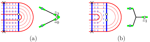
By taking an -extension of , we can ensure that every inner bigon of is contained in a larger domain with the topology of Figure 20(a), and that these domains are separate. Further, we can ensure that every quadrant is contained in a rectangular region. Now consider the effect of a homotopy to a trellis mapping class removing one pair of orbits on the same inner bigons. The resulting trellis and graph locally have the topology of the right of Figure 20(b). The edges and must be expanding, since they forward iterate to a closed segment, and since every quadrant is contained in a rectangular region, for some edge . Therefore and are folded together to obtain the graph representative for . Further, there must be an edge mapping . Hence the entropy of the graph representative of is less than that of , so . Since we can then prune to obtain , we have , hence as required. ∎
We use this to prove that the sufficient condition given for the existence of entropy minimisers in Theorem 4.6 is necessary.
Theorem 4.13 (Non-existence of entropy minimisers)
Let be an irreducible trellis mapping class. Suppose that for every diffeomorphism there is a -extension of which is not minimal. Then there does not exist a diffeomorphism in whose topological entropy equals .
Proof.
Suppose there is an -extension of which is not minimal. Let be a transitive -extension of , and be a further extension such that every non-wandering segment of crosses a regular domain of . Then we have entropy bound .
Take to be a minimal supertrellis of for which the opposite sides of every regular region bound a stable or unstable region. Then every nonwandering segment of enters a stable or unstable region of . Prune to obtain a trellis mapping class which forces satisfying the conditions of Theorem 4.6. Then , but by Lemma 4.12, . Combining these inequalities we have as required. ∎
The results of this section show that many fundamental properties of an irreducible trellis type depends on whether there is a diffeomorphism for which . If such a diffeomorphism exists, then the entropy of the trellis type is carried in a uniformly hyperbolic diffeomorphism, but is fragile in the sense that any pruning will reduce the Nielsen entropy, and any diffeomorphism for which some extension is non-minimal must have strictly greater topological entropy. If no such diffeomorphism exists, every diffeomorphism in the trellis type has an extension which is non-minimal, but pruning this extension gives a trellis type for which the entropy is still greater than the Nielsen entropy of .
References
- [BH95] Mladen Bestvina and Michael Handel. Train-tracks for surface homeomorphisms. Topology, 34(1):109–140, 1995.
- [Boy99] Philip L. Boyland. Isotopy stability of dynamics on surfaces. In Marcy Barge and Krystyna Kuperberg, editors, Geometry and Topology in Dynamics, number 246 in Contemporary Mathmatics, pages 17–45, Providence, Rhode Island, 1999. American Mathematical Society.
- [CB88] A. Casson and S. Bleiler. Automorphisms of surfaces, after Nielsen and Thurston, volume 9 of London Mathematical Society Student Texts. Cambridge University Press, 1988.
- [Col] Pieter Collins. Dynamics of surface diffeomorphisms relative to homoclinic and heteroclinic orbits. To appear in Dynamical Systems: An International Journal.
- [Col99] Pieter Collins. Dynamics forced by surface trellises. In Marcy Barge and Krystyna Kuperberg, editors, Geometry and Topology in Dynamics, number 246 in Contemporary Mathmatics, pages 65–86, Providence, Rhode Island, 1999. American Mathematical Society.
- [Col01] Pieter Collins. Relative periodic point theory. Topology Appl., 115(1):97–114, 2001.
- [Col02] Pieter Collins. Symbolic dynamics from homoclinic tangles. Intern. J. Bifur. Chaos, 12(3):605–617, 2002.
- [dCH02] André de Carvalho and Toby Hall. The forcing relation for horseshoe braind types. Experimental Math., 11(2):271–288, 2002.
- [Fat90] Albert Fathi. Homotopical stability of pseudo-anosov diffeomorphisms. Ergodic Theory Dynamical Systems, 10(2):387–294, 1990.
- [FM93] John Franks and Michael Misiurewicz. Cycles for disk homeomorphisms and thick trees. In Nielsen Theory and Dynamical Systems, number 152 in Contemporary Mathematics, pages 69–139, 1993.
- [Han85] Michael Handel. Global shadowing of pseudo-Anosov homeomorphisms. Ergodic Theory Dynamical Systems, 5(3):373–377, 1985.
- [Jia83] Boju Jiang. Lectures on Nielsen Fixed Point Theory. Number 14 in Contemporary Mathematics. American Mathematical Society, Providence, Rhode Island, 1983.
- [Jia96] Boju Jiang. Estimation of the number of periodic orbits. Pacific J. Math., 172:151–185, 1996.