The Integer Valued SU(3) Casson Invariant for Brieskorn spheresThanks: The first author was partially supported by a grant from the Natural Sciences and Engineering Research Council of Canada. The second author acknowledges support from NSF under grant no. DMS-0072564. The third author would like to thank the NSF for its support under grant no. DMS-0202148

Hans U. Boden Address: Department of Math & Stats, McMaster University, Hamilton, Ontario L8S 4K1 Canada Email address: boden@mcmaster.ca , Christopher M. Herald Address: Department of Mathematics, University of Nevada, Reno Nevada 89557 Email address: herald@unr.edu and Paul A. Kirk Address: Department of Mathematics, Indiana University, Bloomington, Indiana 47405 Email address: pkirk@indiana.edu

Date: Sept. 1, 2003

Abstract.

We develop techniques for computing the integer valued $SU(3)$ Casson invariant defined in [6]. Our method involves resolving the singularities in the flat moduli space using a twisting perturbation and analyzing its effect on the topology of the perturbed flat moduli space. These techniques, together with Bott-Morse theory and the splitting principle for spectral flow, are applied to calculate $\tau_{SU(3)}(\Sigma)$ for all Brieskorn homology spheres.

1. Introduction

In this article we compute the integer valued $SU(3)$ Casson invariant $\tau_{SU(3)}$ for Brieskorn spheres $\Sigma(p,q,r)$ . Computations of $\tau_{SU(3)}(\Sigma(2,q,r))$ appear in [6], and we extend those computations to all Brieskorn spheres.

If $\Sigma$ is a 3-dimensional homology sphere whose flat $SU(3)$ moduli space is nondegenerate and 0-dimensional, then the integer valued $SU(3)$ Casson invariant $\tau_{SU(3)}(\Sigma)$ is simply a signed count of the points in the irreducible stratum of the flat moduli space. On the other hand, if the moduli space has positive dimension and is nondegenerate in the sense of Bott and Morse (or more generally if its lift to the based moduli space is nondegenerate), then one can apply standard (equivariant) Morse theoretic techniques to compute the invariant $\tau_{SU(3)}(\Sigma)$ (see [4]).

The family of computations given here represents the first successful attempt to compute the invariant $\tau_{SU(3)}(\Sigma)$ for manifolds $\Sigma$ with truly singular moduli spaces. Even in the connected sum theorem of [4] where one encounters components of mixed type in the moduli space (i.e., components containing both irreducible and reducible gauge orbits), when lifted to the based moduli space, these components become nondegenerate and one can apply equivariant Bott-Morse theory to determine the invariant $\tau_{SU(3)}$ . In contrast, the flat $SU(3)$ moduli space of the Brieskorn spheres considered in this paper are singular even when lifted to the based moduli space. Thus the perturbation techniques presented here go beyond the standard theory and in fact provide a new approach to transversality issues that may well apply more generally.

The new approach involves a combination of manifold decomposition and Mayer-Vietoris techniques and traditional holonomy perturbations. Simply put, our idea is to construct a special type of perturbation (called the twisting perturbation) and analyze its effect on the moduli space. We prove that under such perturbations, the moduli space becomes nondegenerate and we express the invariant $\tau_{SU(3)}$ in terms of the topology of the perturbed moduli space and the spectral flow of the odd signature operator.

The remainder of this paper is divided into five sections. Section 2 presents a detailed description of the $SU(3)$ representation varieties of Brieskorn spheres. Corresponding results for knot complements are given in Section 3. Section 4 introduces the twisting perturbations and describes their effect on the moduli spaces. Section 5 presents spectral flow computations based on a splitting argument, and Section 6 presents a lattice point count which provides numerical calculations of $\tau_{SU(3)}$ for families of Brieskorn spheres $\Sigma(p,q,r)$ , including all homology 3-spheres obtained by Dehn surgery on a $(p,q)$ torus knot. The rest of the introduction is devoted to outlining the main argument.

Recall first that if $\pi$ is a (finitely presented) group, a representation $\alpha\colon\pi\to SU(3)$ is irreducible if no nontrivial linear subspace of ${\mathbb{C}}^{3}$ is invariant under $\alpha(g)$ for all $g\in\pi$ . This is equivalent to the condition that the stabilizer of $\alpha$ with respect to the conjugation action equals the center of $SU(3)$ . Otherwise, $\alpha$ is reducible and its image can be conjugated to lie in the subgroup $S(U(2)\times U(1))$ .

Suppose that $\Sigma$ is a homology 3-sphere and let $R(\Sigma,SU(3))$ be the set of conjugacy classes of representations $\alpha\colon\pi_{1}(\Sigma)\to SU(3)$ . Then $R(\Sigma,SU(3))$ is a real algebraic variety homeomorphic to the moduli space ${\mathcal{M}}(\Sigma)$ of flat $SU(3)$ connections on $\Sigma$ . We denote by $R^{*}(\Sigma,SU(3))$ the subspace of conjugacy classes of irreducible representations and by ${\mathcal{M}}^{*}(\Sigma)$ the subspace of irreducible flat connections.

The integer valued $SU(3)$ Casson invariant $\tau_{SU(3)}(\Sigma)$ is defined in [6] and gives an algebraic count of the conjugacy classes of irreducible representations of $\pi_{1}(\Sigma)$ , with a correction term involving the reducible representations. More precisely, the flatness equations are perturbed so that the flat moduli space becomes nondegenerate, and gauge orbits of irreducible perturbed flat connections are counted with sign given by the spectral flow of the $su(3)$ odd signature operator. The resulting integer depends on the perturbation used, and to compensate for this we add a correction term defined in terms of the reducible stratum.

For $\Sigma=\Sigma(p,q,r)$ the Brieskorn sphere, the analysis of [2] shows that $R(\Sigma,SU(3))$ is a union of path components, each of which is homeomorphic to either an isolated point or a 2-sphere. More precisely, we will show that each path component is one of the following four types:

Type Ia:: Isolated conjugacy classes of irreducible representations.
Type IIa:: Smooth 2-spheres, each parameterizing a family of conjugacy classes of irreducible representations.
Type Ib:: Isolated conjugacy classes of nontrivial reducible representations.
Type IIb:: Pointed 2-spheres, each parameterizing a family of conjugacy classes of representations, exactly one of which is reducible.

The main result in this paper is the following theorem (Theorem 6.2), which describes how each of the component types contributes to the $SU(3)$ Casson invariant. This, together with enumerations of the components of each type, enable us to calculate the invariant for a variety of Brieskorn spheres $\Sigma(p,q,r)$ . The results of these computations can be found in Tables 1 and 2.

Theorem. Type Ia, IIa, Ib, and IIb components each contribute +1, +2, 0, and +2, respectively, to the integer valued $SU(3)$ Casson invariant $\tau_{SU(3)}(\Sigma(p,q,r))$ .

We conclude the introduction by outlining the proof of this theorem. Components of Type Ia are regular and remain so after small perturbations. The sign attached to each such point is positive by the results of [2], and so computing the contribution of the Type Ia points to $\tau_{SU(3)}(\Sigma)$ reduces to an enumeration problem. This is carried out in Section 6.

Components of Type IIa are nondegenerate critical submanifolds of the Chern-Simons function. Bott-Morse theory, together with a spectral flow computation, implies that each such component contributes $\chi(S^{2})=2$ to $\tau_{SU(3)}(\Sigma)$ . Thus the computation of the contribution of the Type IIa components to $\tau_{SU(3)}(\Sigma)$ is also reduced to an enumeration problem which is solved in Section 6.

Components of Type Ib do not contribute to $\tau_{SU(3)}(\Sigma)$ (although they do enter into the calculations of the invariant $\lambda_{SU(3)}$ given in [5]).

The only remaining issue is to calculate the contribution of components of Type IIb. This requires some sophisticated techniques that go beyond those of [6], where one can find computations of $\tau_{SU(3)}$ for Brieskorn spheres of the form $\Sigma(2,q,r)$ (whose representation varieties do not contain any Type IIb components). The problem is that Type IIb components are singular in a strong sense: even their lifts to the based moduli space are singular. We introduce a perturbation which resolves these singularities and then carefully analyze its effect on the topology of the moduli space. We prove that after applying the perturbation, each pointed 2-sphere resolves into two pieces, one isolated gauge orbit of reducible connections and the other a smooth, nondegenerate 2-sphere of gauge orbits of irreducible connections (similar to a Type IIa component).

In defining the perturbation, we regard one of the singular fibers of the Seifert fibration $\Sigma\to S^{2}$ as a knot in $\Sigma$ and perturb the flatness equations in a small neighborhood of this knot. Consequently, perturbed flat connections are seen to be flat on the knot complement, and we study the perturbed flat moduli space in terms of the $SU(3)$ representation space of this knot complement. Basically, the perturbed flat moduli space on $\Sigma$ is obtained from the flat moduli space of the knot complement by replacing the condition “meridian is sent to the identity” by a condition of the form “the meridian and longitude are related by a certain equation.”

Having resolved the singularities in the Type IIb components, we then determine the contribution of the reducible, perturbed flat connection to the correction term. This is given by the spectral flow (with ${\mathbb{C}}^{2}$ coefficients) of the odd signature operator. To calculate this we prove a splitting theorem for spectral flow determined by the decomposition of $\Sigma$ into a knot complement and a solid torus.

Notation. If $\pi$ is a discrete group and $\alpha\colon\pi\to G$ is a representation, we denote the stabilizer subgroup of $\alpha$ by

\Gamma_{\alpha}=\{g\in G\mid g\alpha g^{-1}=\alpha\}.

If $G$ is a Lie group, the orbit of $\alpha$ under conjugation is smooth and diffeomorphic to the homogeneous manifold $G/\Gamma_{\alpha}$ . We denote the representation variety

R(\pi,G)=\operatorname{Hom}(\pi,G)/\text{conjugation}.

Given a representation $\alpha\colon\pi\to G,$ we denote its conjugacy class by $[\alpha].$ Given a manifold $X$ , we denote by $R(X,G)$ the representation variety of the fundamental group $\pi_{1}(X).$

2. SU(3) representation spaces of Brieskorn spheres

In this section, we identify the components of the $SU(3)$ representation varieties of Brieskorn spheres $\Sigma$ , both as topological spaces and as varieties with their Zariski tangent spaces. Crucial to our discussion are computations of the twisted cohomology groups which reflect the local structure of the representation varieties. The global structure of the representation variety is presented in Theorem 2.6, which gives a complete classification of the different path components of $R(\Sigma,SU(3))$ .

Refer to caption — Figure 1. A surgery description of the Brieskorn manifold $\Sigma(p,q,r)$ indicating the Wirtinger generators $x,y,z,$ and $h$ for $\pi_{1}(\Sigma)$ .

2.1. Brieskorn spheres

Given integers $p,q,r$ , set

\Sigma(p,q,r)=\{(x,y,z)\in{\mathbb{C}}^{3}\mid x^{p}+y^{q}+z^{r}=0\}\cap S^{5}.

If $p,q,r$ are pairwise relatively prime then $\Sigma(p,q,r)$ is a homology 3-sphere and has surgery description in Figure 1 (see [22] for details). Here, $a,b,c$ satisfy

(2.1)

aqr+bpr+cpq=1.

The resulting manifold $\Sigma(p,q,r)$ is independent of $a,b,c$ , up to orientation preserving homeomorphism. Without loss of generality we assume that $p$ and $q$ are odd.

Proposition 2.1.

The numbers $a$ and $b$ can be chosen to be equal.

Proof.

Since $p,q,$ and $r$ are pairwise relatively prime, $r(p+q)$ and $pq$ are relatively prime. Thus there are integers $a$ and $c$ such that

ar(p+q)+cpq=1,

which is equivalent to the condition (2.1) with $b=a$ . ∎

Fix integers $a$ and $c$ as above. Note that since $p$ and $q$ are both odd, $c$ must also be odd. A presentation for the fundamental group of $\Sigma(p,q,r)$ is

(2.2)

\pi_{1}\big(\Sigma(p,q,r)\big)=\langle x,y,z,h\mid~x^{p}=y^{q}=h^{a},~z^{r}=h^{c},~xyz=1,h\mbox{ is central}\rangle,

where $x,y,z$ and $h$ are the Wirtinger generators indicated in Figure 1.

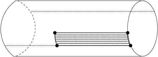
Whenever $p,q,$ and $r$ are clear from the context, we drop them from the notation and denote the Brieskorn sphere by $\Sigma$ . A regular neighborhood of the singular $r$ -fiber in $\Sigma$ is a solid torus whose boundary torus $T$ splits the Brieskorn sphere $\Sigma=Y\cup_{T}Z$ , where $Y=D^{2}\times S^{1}$ is the solid torus and $Z=\Sigma-Y$ is its complement. Alternatively, $Z$ is the complement of an open tubular neighborhood of the core of the $\left(\frac{r}{c}\right)$ curve in $\Sigma$ and depicted in Figure 1. With regard to the natural peripheral structure thus obtained on $Z$ , its fundamental group has presentation

(2.3)

\pi_{1}(Z)=\langle x,y,h\mid~x^{p}=y^{q}=h^{a},h\mbox{ is central}\rangle.

In terms of these generators, the meridian and longitude are represented by

(2.4)

\mu=(xy)^{r}h^{c}\qquad\hbox{and}\qquad\lambda=(xy)^{pq}h^{-(p+q)a}.

Then $\mu$ generates the abelianization of $\pi_{1}(Z)$ , and one can check that in $H_{1}(Z)$ ,

(2.5)

[x]=aq[\mu],\ [y]=ap[\mu],\ [h]=pq[\mu],\text{ and }[\lambda]=0.

2.2. Decompositions of $\boldsymbol{su(3)}$

In this subsection, we examine the restriction of the adjoint representation of $SU(3)$ on its Lie algebra $su(3)$ to various subgroups.

Consider first the subgroup

SU(2)\times\{1\}=\left\{\begin{pmatrix}A&0\\ 0&1\end{pmatrix}\,\Bigm|A\in SU(2)\right\}\subset SU(3).

Then $su(3)$ decomposes invariantly with respect to the adjoint action of $SU(2)\times\{1\}$ as

(2.6)

su(3)=su(2)\oplus{\mathbb{C}}^{2}\oplus{\mathbb{R}},

where $SU(2)\times\{1\}$ acts by the adjoint action on $su(2)$ , by the defining representation on ${\mathbb{C}}^{2}$ , and trivially on ${\mathbb{R}}$ .

More generally, consider the subgroup

S(U(2)\times U(1))=\left\{\begin{pmatrix}A&0\\ 0&\det{A}^{-1}\end{pmatrix}\,\Bigm|\,A\in U(2)\right\}\subset SU(3).

The decomposition of the Lie algebra $su(3)$ takes the form

(2.7)

su(3)=s(u(2)\times u(1))\oplus{\mathbb{C}}^{2},

where $S(U(2)\times U(1))$ acts on the first factor via the adjoint representation and on the second factor by

\left[\begin{array}[]{ccc}ta&tb&0\\ -t\bar{b}&t\bar{a}&0\\ 0&0&t^{-2}\end{array}\right]\cdot\left[\begin{array}[]{c}z_{1}\\ z_{2}\end{array}\right]=t^{3}\left[\begin{array}[]{c}az_{1}+bz_{2}\\ -\bar{b}z_{1}+\bar{a}z_{2}\end{array}\right]\ (|t|=1,\ |a|^{2}+|b|^{2}=1).

There is a canonical isomorphism $S(U(2)\times U(1))\cong U(2).$ However, the action of $S(U(2)\times U(1))$ on ${\mathbb{C}}^{2}$ is not the standard $U(2)$ action, even though its restriction to the subgroup $SU(2)\times\{1\}$ is standard.

Every $SU(3)$ matrix is diagonalizable. We parameterize the diagonal matrices using the map $\Phi\colon{\mathbb{R}}^{2}\to SU(3)$ given by

(2.8)

\Phi(u,v)=\left[\begin{array}[]{ccc}e^{i(u+v)}&0&0\\ 0&e^{i(-u+v)}&0\\ 0&0&e^{-2iv}\end{array}\right].

With respect to the decomposition (2.7), the matrix $\Phi(u,v)$ acts on ${\mathbb{C}}^{2}$ by

\Phi(u,v)\left[\begin{array}[]{c}z_{1}\\ z_{2}\end{array}\right]=e^{3iv}\left[\begin{array}[]{c}e^{iu}z_{1}\\ e^{-iu}z_{2}\end{array}\right].

Note that the centralizer of $S(U(2)\times U(1))$ is $\{\Phi(0,v)\}$ , and this circle acts trivially on $s(u(2)\times u(1))$ and with weight three on ${\mathbb{C}}^{2}$ .

2.3. Cohomology calculations

In this subsection, we give computations of $H^{i}(\Sigma;su(3)_{\alpha})$ , where $\alpha\colon\pi_{1}(\Sigma)\to SU(3)$ is a representation and $SU(3)$ acts on its Lie algebra $su(3)$ via the adjoint representation. First, we establish some notation and recall some basic facts. Let $X$ be a cell complex, $G$ a Lie group, $V$ a vector space on which $G$ acts, and $\alpha\colon\pi_{1}(X)\to G$ a representation. Denote by $V_{\alpha}$ the local coefficient system determined by $\alpha$ and by $H^{i}(X;V_{\alpha})$ the $i$ -th cohomology group of $X$ with twisted coefficients in $V_{\alpha}.$ Although some of the cohomology groups we consider have natural complex structures, we use the notation $\dim(H)$ to refer to the dimension of $H$ as a real vector space.

Given a finite complex $X$ and representation $\alpha\colon\pi=\pi_{1}(X)\longrightarrow GL(V)$ , we can identify $H^{i}(X;V_{\alpha})\cong H^{i}(\pi;V_{\alpha})$ for $i=0,1$ . Group cohomology $H^{*}(\pi;V_{\alpha})$ can be computed from the reduced bar resolution. In this model, the space of (twisted) $i$ -cochains is given by a set of functions:

C^{0}(\pi;V)=V,\ C^{i}(\pi;V)=\{f\colon\stackrel{{\scriptstyle\text{\tiny$i$ terms}}}{{\pi\times\cdots\times\pi}}\longrightarrow V\},i>0.

We will only need the formulas for the $0$ -th and $1$ -st coboundary operators,

d^{0}(v)(\gamma)=(\gamma-1)\cdot v,\ d^{1}(f)(\gamma_{1},\gamma_{2})=f(\gamma_{1})+\gamma_{1}\cdot f(\gamma_{2})-f(\gamma_{1}\gamma_{2}).

The Fox calculus provides a means to calculate the 1-cocycles, i.e. the solutions $f\in C^{1}(\pi;V_{\alpha})$ to the equation $d^{1}(f)=0$ . Given a presentation $\pi=\langle x_{1},\ldots,x_{m}\mid r_{1},\ldots,r_{n}\rangle$ , the Fox derivative of a relation $r_{j}$ with respect to a cocycle $f$ is the element of $V$ obtained by using the equation $f(\gamma_{1}\gamma_{2})=f(\gamma_{1})+\gamma_{1}\cdot f(\gamma_{2})$ inductively to express $0=f(1)=f(r_{j})$ in terms of $X_{i}=f(x_{i})$ . Note that the map $f\mapsto(f(x_{1}),\ldots,f(x_{n}))$ is injective on 1-cocyles. Most of our computations are given in terms of group cohomology, but occasionally we will make use of topological tools such as Poincaré duality and the Euler characteristic.

We now explain the relationship between representation varieties and these cohomology groups. Suppose that $G$ is a compact Lie group, acting on its Lie algebra ${\mathfrak{g}}$ via the adjoint action, and $\pi$ is a finitely presented group. Then the Zariski tangent space to (the algebraic variety) $R(\pi,G)$ at the conjugacy class of a representation $\alpha\colon\pi\to G$ is isomorphic to $H^{1}(\pi;{\mathfrak{g}}_{\alpha})$ . Moreover, $\dim H^{0}(\pi;{\mathfrak{g}}_{\alpha})=\dim\Gamma_{\alpha},$ where $\Gamma_{\alpha}\subset G$ denotes the stabilizer subgroup of $\alpha$ under the conjugation action of $G$ on $\operatorname{Hom}(\pi,G)$ . Equivalently, $\Gamma_{\alpha}$ equals the centralizer of $\operatorname{im}(\alpha)$ .

The Kuranishi map embeds a neighborhood of $[\alpha]$ in $R(\pi,G)$ into its Zariski tangent space modulo $\Gamma_{\alpha}$ . In particular if $H^{1}(\pi;{\mathfrak{g}}_{\alpha})=0$ , then $[\alpha]$ is an isolated point in $R(\pi,G)$ (although the converse is sometimes false). We say that $[\alpha]\in R(\pi,G)$ is a smooth point if a neighborhood of $[\alpha]$ in $R(\pi,G)$ is homeomorphic to $H^{1}(\pi,{\mathfrak{g}}_{\alpha})$ ; otherwise $[\alpha]$ is called a singular point.

We are mostly interested in the case when $G=SU(3)$ and $V=su(3)$ . For reducible representations, we are interested in the case $G=SU(2)$ and $V=su(2)$ or ${\mathbb{C}}^{2}$ . To see why, note that up to conjugation, any reducible representation $\alpha\colon\pi_{1}(\Sigma)\to SU(3)$ has image in the subgroup $S(U(2)\times U(1)).$ Since $\Sigma$ is a homology sphere, it follows that $\alpha$ has image in $SU(2)\times\{1\}.$ Using the decomposition (2.6) we conclude that

H^{i}(\Sigma;su(3)_{\alpha})=H^{i}(\Sigma;su(2)_{\alpha})\oplus H^{i}(\Sigma;{\mathbb{C}}^{2}_{\alpha})\oplus H^{i}(\Sigma;{\mathbb{R}}),

where the first cohomology group has coefficients $su(2)$ twisted via the adjoint action (viewing $\alpha$ as an $SU(2)$ representation), the second has coefficients ${\mathbb{C}}^{2}$ twisted by the standard representation, and the last has untwisted real coefficients.

Proposition 2.2.

Suppose $\alpha\colon\pi_{1}(\Sigma)\to SU(3)$ is a nontrivial representation. Then $\alpha$ has nonabelian image. Moreover:

(i)

If $\alpha$ is irreducible, then $\alpha(h)=e^{2\pi ik/3}I$ for an integer $k$ and

H^{1}(\Sigma;su(3)_{\alpha})=\begin{cases}{\mathbb{R}}^{2}&\text{if $\alpha(x),\alpha(y),$ and $\alpha(z)$ each have three distinct eigenvalues,}\\ 0&\text{otherwise.}\end{cases}

(ii)

If $\alpha$ is reducible and has been conjugated to take values in $SU(2)\times\{1\},$ then

$\alpha(h)=\left[\begin{array}[]{ccc}\pm 1&0&0\\ 0&\pm 1&0\\ 0&0&1\end{array}\right].$

With respect to the splitting $su(3)=su(2)\oplus{\mathbb{C}}^{2}\oplus{\mathbb{R}}$ (see equation (2.7)), we have $H^{0}(\Sigma;su(2)_{\alpha})=0,\ H^{0}(\Sigma;{\mathbb{C}}^{2}_{\alpha})=0,\ H^{1}(\Sigma;su(2)_{\alpha})=0$ and

$H^{1}(\Sigma;{\mathbb{C}}^{2}_{\alpha})=\begin{cases}{\mathbb{C}}^{2}&\text{if $\alpha(h)=I$,}\\ 0&\text{otherwise.}\end{cases}$

Proof.

First note that since $h$ is central in $\pi_{1}(\Sigma)$ , $\alpha(h)$ lies in the centralizer of $\operatorname{im}(\alpha)$ .

We now prove (i). Suppose $\alpha$ is irreducible. Then $\Gamma_{\alpha}$ is the center of $SU(3)$ , and hence is discrete. Thus $\alpha(h)$ is central and $\dim H^{0}(\Sigma;su(3)_{\alpha})=0$ .

Set $\pi=\pi_{1}(\Sigma)$ and let $B^{i}(\pi;su(3)_{\alpha})=\operatorname{im}(d^{i-1})$ be the coboundaries and $Z^{i}(\pi;su(3)_{\alpha})=\ker(d^{i})$ the cocycles in the reduced bar complex. Thus

H^{1}(\pi;su(3)_{\alpha})=Z^{1}(\pi;su(3)_{\alpha})/B^{1}(\pi;su(3)_{\alpha}).

Since $H^{0}(\pi;su(3)_{\alpha})=0,$ $d^{0}$ is injective and $B^{1}(\pi;su(3)_{\alpha})$ has dimension 8. So to compute $H^{1}(\pi;su(3)_{\alpha})$ we only need to determine the dimension of the space $Z^{1}(\pi;su(3)_{\alpha})$ of 1-cocycles.

The Fox calculus identifies $Z^{1}(\pi;su(3)_{\alpha})$ with the set of 4-tuples $(X,Y,Z,H)$ in $su(3)$ satisfying the equations one gets by taking Fox derivatives of the relations in (2.2). For example, the relation $hx=xh$ gives the equation

H+\alpha(h)X=X+\alpha(x)H.

Since $\alpha(h)X=X$ , this reduces to $H=\alpha(x)H.$ Similarly, we get the equations $H=\alpha(y)H$ and $H=\alpha(z)H.$ Since $\alpha$ is irreducible with image generated by $\alpha(x),\alpha(y)$ , and $\alpha(z)$ , these three equations imply $H=0.$

Setting $H=0$ in the remaining equations, we obtain:

$\displaystyle(1+\alpha(x)+\cdots+\alpha(x^{p-1}))X$	$\displaystyle=$	$\displaystyle 0,$
$\displaystyle(1+\alpha(y)+\cdots+\alpha(y^{q-1}))Y$	$\displaystyle=$	$\displaystyle 0,$
$\displaystyle(1+\alpha(z)+\cdots+\alpha(z^{r-1}))Z$	$\displaystyle=$	$\displaystyle 0,$
$\displaystyle X+\alpha(x)Y+\alpha(xy)Z$	$\displaystyle=$	$\displaystyle 0.$

Case 1: $\alpha(x),\alpha(y)$ and $\alpha(z)$ all have three distinct eigenvalues.

Since $\alpha(x)^{p}=\alpha(h)^{a}$ acts as the identity on $su(3)$ via the adjoint action, $su(3)$ decomposes as $T_{x}\oplus U_{x}$ , where $T_{x}$ is the tangent space to the maximal torus containing $\alpha(x)$ and $U_{x}$ is the kernel of the map $1+\alpha(x)+\cdots+\alpha(x)^{p-1}\colon su(3)\to su(3)$ . Note that $T_{x}$ is 2-dimensional (since $\alpha(x)$ has three distinct eigenvalues) and that $\alpha(x)$ acts trivially on $T_{x}$ . It follows from the equations above that $X$ lies in $U_{x}$ . Similar statements hold for $\alpha(y)$ and $\alpha(z)$ . The space of 1-cocycles is therefore a subspace of $U_{x}\oplus U_{y}\oplus U_{z}$ .

Since $\alpha$ is irreducible, $T_{x}\cap T_{y}=0$ . In fact, if $t\in T_{x}\cap T_{y}$ , then exp $(t)\in SU(3)$ stabilizes both $\alpha(x)$ and $\alpha(y)$ and hence stabilizes $\alpha$ . Thus $U_{x}\cap U_{y}$ is 4-dimensional, and therefore $U_{x}+U_{y}$ is 8-dimensional, i.e. $U_{x}+U_{y}=su(3)$ .

Since $\alpha(x)^{-1}$ preserves the decomposition $su(3)=T_{x}\oplus U_{x}$ and acts as an isomorphism on each factor, the linear map

U_{x}\oplus U_{y}\to su(3),\ (X,Y)\mapsto\alpha(x)^{-1}X+Y

is onto. Thus the linear map

(X,Y,Z)\mapsto\alpha(x)\big(\alpha(x)^{-1}X+Y\big)+\alpha(xy)Z=X+\alpha(x)Y+\alpha(xy)Z

is also onto. Its kernel is just the space of 1-cocycles, and so $\dim Z^{1}(\pi;su(3)_{\alpha})=10$ . Hence $\dim H^{1}(\pi;su(3)_{\alpha})=10-8=2$ .

Case 2: One of $\alpha(x),\alpha(y)$ and $\alpha(z)$ has a double eigenvalue.

We first show that at most one of $\alpha(x),\alpha(y),$ and $\alpha(z)$ can have a double eigenvalue. For example, if both $\alpha(x)$ and $\alpha(y)$ had a double eigenvalue, then the intersection of the corresponding eigenspaces would determine a linear subspace invariant under $\alpha(x)$ , $\alpha(y)$ , and $\alpha(z)=\alpha(xy)^{-1}$ , contradicting the irreducibility of $\alpha.$

So assume that $\alpha(x)$ has a double eigenvalue and $\alpha(y)$ and $\alpha(z)$ have three distinct eigenvalues (the proofs of the other cases work the same way). Under the adjoint action of $\alpha(x)$ , $su(3)$ decomposes as ${\mathbb{C}}^{2}\oplus{\mathbb{R}}^{4}$ , where $\alpha(x)$ acts trivially on ${\mathbb{R}}^{4}$ and by multiplication by a nontrivial $p$ -th root of unity on ${\mathbb{C}}^{2}$ . Thus we see that $X$ now lies in a (real) 4-dimensional subspace ${\mathbb{C}}^{2}\subset su(3)$ . Arguing as before, we conclude that $\dim Z^{1}(\pi;su(3)_{\alpha})=4+6+6-8=8$ , from which it follows that

\dim H^{1}(\pi;su(3)_{\alpha})=\dim Z^{1}(\pi;su(3)_{\alpha})-\dim B^{1}(\pi;su(3)_{\alpha})=8-8=0.

These two cases complete the proof of (i) because irreducibility of $\alpha$ precludes any other possibility. To see this, suppose one of $\alpha(x),\alpha(y)$ or $\alpha(z)$ were central, say $\alpha(x)$ , then the relation $xyz=1$ would imply that $\alpha(y)$ commutes with $\alpha(z)$ , and hence that $\alpha$ is abelian. This would imply $\alpha$ is trivial (and in particular reducible).

In proving (ii), we regard $\alpha$ as an $SU(2)$ representation. Irreducibility of $\alpha$ (as an $SU(2)$ representation) implies that $H^{0}(\Sigma;su(2)_{\alpha})=0$ and $\alpha(h)=\pm I$ . The fact that $H^{1}(\Sigma;su(2)_{\alpha})=0$ for Brieskorn spheres is well-known (see [12]). Nontriviality of $\alpha$ implies $H^{0}(\Sigma;{\mathbb{C}}^{2}_{\alpha})=0$ , and that leaves $H^{1}(\Sigma;{\mathbb{C}}^{2}_{\alpha})$ , which we determine with another application of the Fox calculus. The only difference is that we use the defining representation instead of the adjoint representation. In particular, $-I\in SU(2)$ acts nontrivially.

Suppose then that $(X,Y,Z,H)$ is a 4-tuple of vectors in ${\mathbb{C}}^{2}$ satisfying the equations one gets by taking Fox derivatives of the relations in (2.2). There are two cases.

Case 1: $\alpha(h)=I.$

As before, $H=0$ and $\alpha(x)$ acts by multiplication by a nontrivial $p$ -th root of unity in each of the two complex factors. Consequently $(1+\alpha(x)+\cdots+\alpha(x^{p-1}))X=0$ for all $X\in{\mathbb{C}}^{2}.$ Similar statements hold for $Y$ and $Z$ and it follows that $(X,Y,Z,H)$ is a 1-cocycle provided $H=0$ and $X+\alpha(x)Y+\alpha(xy)Z=0.$ One can check that the last equation imposes four independent conditions, hence $\dim Z^{1}(\pi;{\mathbb{C}}^{2}_{\alpha})=4+4+4-4=8$ , and it follows that

\dim H^{1}(\pi;{\mathbb{C}}^{2}_{\alpha})=\dim Z^{1}(\pi;{\mathbb{C}}^{2}_{\alpha})-\dim B^{1}(\pi;{\mathbb{C}}^{2}_{\alpha})=8-4=4.

Case 2: $\alpha(h)=-I.$

In this case, $\alpha(h)$ acts on ${\mathbb{C}}^{2}$ by multiplication by $-1$ and it is no longer true that $H=0.$ Instead, we find that $H$ determines $X$ by the equation $(1-\alpha(h))X=(1-\alpha(x))H$ and similarly for $Y$ and $Z$ . An easy check shows that all the remaining equations are automatically satisfied, and since $H$ is an arbitrary element in ${\mathbb{C}}^{2},$ it follows that $\dim Z^{1}(\pi;{\mathbb{C}}^{2}_{\alpha})=4$ and

\dim H^{1}(\pi;{\mathbb{C}}^{2}_{\alpha})=\dim Z^{1}(\pi;{\mathbb{C}}^{2}_{\alpha})-\dim B^{1}(\pi;{\mathbb{C}}^{2}_{\alpha})=4-4=0

as claimed. ∎

2.4. The representation variety R( ${\boldsymbol{\Sigma}}$ ,SU(3))

In this subsection, we classify the different path components of the representation variety $R(\Sigma,SU(3)).$ To start off, we show that every component contains at most one conjugacy class of reducible representations.

Proposition 2.3.

If $\alpha_{t},\ t\in[0,1],$ is a continuous path of $SU(3)$ representations of $\pi_{1}(\Sigma)$ with $\alpha_{0}$ and $\alpha_{1}$ both reducible, then $\alpha_{0}$ and $\alpha_{1}$ are conjugate. Consequently, every path component of $R(\Sigma,SU(3))$ contains at most one conjugacy class of reducible representations.

Proof.

For the trivial representation $\theta$ , $H^{1}(\Sigma;su(3)_{\theta})=H^{1}(\Sigma;{\mathbb{R}}^{8})=0$ , so $[\theta]$ is isolated. Thus we assume that $\alpha_{t}$ is nontrivial for all $t$ . If $\alpha_{0}(h)\neq I$ , then Proposition 2.2 implies that $[\alpha_{0}]$ is isolated. So we can assume that $\alpha_{0}(h)=I$ . The continuous function $t\mapsto\operatorname{\it tr}(\alpha_{t}(h))$ takes values in the discrete set $\{3,-1,3e^{2\pi i/3},3e^{4\pi i/3}\}$ by Proposition 2.2. It follows that $\alpha_{t}(h)=I$ for all $t$ . The relations (2.2) then imply that $\alpha_{t}(x),\ \alpha_{t}(y),$ and $\alpha_{t}(z)$ are conjugate to fixed $p$ -th, $q$ -th, and $r$ -th roots of unity in $SU(3)$ for all $t$ . (To see this, use continuity and the fact that the trace map $\operatorname{\it tr}\colon SU(3)\to{\mathbb{C}}$ distinguishes conjugacy classes and sends the set $\{A\in SU(3)\mid A^{k}=I\}$ of all $k$ -th roots of unity into a discrete set.)

Since $\alpha_{0}$ and $\alpha_{1}$ are both reducible and $SU(3)$ is path connected, we may assume that the path $\alpha_{t}$ is conjugated so that $\alpha_{0}$ and $\alpha_{1}$ take values in $SU(2)\times\{1\}$ . Thus $\alpha_{0}(x)$ and $\alpha_{1}(x)$ each have one eigenvalue equal to 1. But since $\alpha_{0}(x)$ and $\alpha_{1}(x)$ are conjugate (in $SU(3)$ ), the other two eigenvalues of $\alpha_{0}(x)$ and $\alpha_{1}(x)$ coincide. The same argument applies to $y$ and $z$ .

It is well-known that the conjugacy class $[\beta]$ of a representation $\beta\colon\pi_{1}(\Sigma)\to SU(2)$ of a Brieskorn sphere is completely determined by the eigenvalues of $\beta(x),\beta(y),$ and $\beta(z)$ (see [12]). Hence $\alpha_{0}$ and $\alpha_{1}$ are conjugate as $SU(2)$ and hence also as $SU(3)$ representations. ∎

Proposition 2.4.

Every path component of $R(\Sigma,SU(3))$ is either an isolated point, a smooth 2-sphere consisting of conjugacy classes of irreducible representations, or a pointed 2-sphere, which is smooth except for exactly one singular point, the conjugacy class of a reducible representation.

Proof.

It is proved in [2, 16] that each path component of $R(\Sigma,SU(3))$ is either an isolated point or a topological 2-sphere. In the case of an isolated point, there is nothing to prove, so assume the path component is a 2-sphere. Any conjugacy class $[\alpha]$ of irreducible representations lying on such a component must have nonzero Zariski tangent space, and Proposition 2.2 then implies $H^{1}(\Sigma;su(3)_{\alpha})\cong{\mathbb{R}}^{2}$ and we conclude that $[\alpha]$ is indeed a smooth point of $R(\Sigma,SU(3))$ . On the other hand, Proposition 2.3 shows that every path component of $R(\Sigma,SU(3))$ contains at most one conjugacy class of reducible representations. For a pointed 2-sphere component, the conjugacy class $[\beta]$ of reducible representations is never a smooth point, since Proposition 2.2 shows its Zariski tangent space is $H^{1}(\Sigma;su(3)_{\beta})\cong{\mathbb{R}}^{4}$ . (Note that the hypothesis on $\beta$ implies that $H^{1}(\Sigma;su(3)_{\beta})\neq 0$ , and then Proposition 2.2 shows that $\beta(h)=I$ .) ∎

The next proposition shows that the pointed 2-spheres are in one-to-one correspondence with the nontrivial reducible representations sending $h$ to the identity.

Proposition 2.5.

Given a nontrivial reducible representation $\alpha\colon\pi_{1}(\Sigma)\to SU(3),$ the following are equivalent:

(i)

$\alpha(h)=I$ ,
(ii)

$H^{1}(\Sigma;{\mathbb{C}}^{2}_{\alpha})\neq 0$ ,
(iii)

There exists a family of irreducible $SU(3)$ representations limiting to $\alpha$ .

The collection of pointed 2-spheres in $R(\Sigma,SU(3))$ are therefore in one-to-one correspondence with conjugacy classes of nontrivial reducible representations $\alpha\colon\pi_{1}(\Sigma)\to SU(3)$ with $\alpha(h)=I.$ Further, $\operatorname{\it tr}\alpha(z)$ is constant along a pointed 2-sphere.

Proof.

The statement (i) $\Leftrightarrow$ (ii) follows from Proposition 2.2, (ii). The implication (iii) $\Rightarrow$ (ii) follows because the Kuranishi map locally embeds $R(\Sigma,SU(3))$ near $[\alpha]$ into its Zariski tangent space $H^{1}(\Sigma;su(3)_{\alpha})$ modulo $\Gamma_{\alpha}$ , and the Zariski tangent space equals $H^{1}(\Sigma;{\mathbb{C}}^{2}_{\alpha})$ by Proposition 2.2.

For the implication (i) $\Rightarrow$ (iii), notice that a representation $\alpha\colon\pi_{1}(\Sigma)\to SU(3)$ satisfying $\alpha(h)=I$ uniquely determines an $SU(3)$ representation of the (free) group $F=\langle x,y,z\mid xyz=1\rangle$ . Fix three conjugacy classes ${\boldsymbol{a}},{\boldsymbol{b}},{\boldsymbol{c}}$ in $SU(3)$ and consider the space ${\mathcal{M}}_{{\boldsymbol{a}}{\boldsymbol{b}}{\boldsymbol{c}}}$ consisting of conjugacy classes of representations $\alpha\colon F\to SU(3)$ with $\alpha(x)\in{\boldsymbol{a}},\ \alpha(y)\in{\boldsymbol{b}},$ and $\alpha(z)\in{\boldsymbol{c}}.$ In [16], Hayashi gives necessary and sufficient conditions on ${\boldsymbol{a}},{\boldsymbol{b}},{\boldsymbol{c}}$ for ${\mathcal{M}}_{{\boldsymbol{a}}{\boldsymbol{b}}{\boldsymbol{c}}}$ to be nonempty. The resulting inequalities (18 in all) determine a convex, 6-dimensional polytope $P$ parameterizing all triples $({\boldsymbol{a}},{\boldsymbol{b}},{\boldsymbol{c}})$ with ${\mathcal{M}}_{{\boldsymbol{a}}{\boldsymbol{b}}{\boldsymbol{c}}}\neq\varnothing.$ Hayashi observes further that ${\mathcal{M}}_{{\boldsymbol{a}}{\boldsymbol{b}}{\boldsymbol{c}}}$ is a 2-sphere whenever $({\boldsymbol{a}},{\boldsymbol{b}},{\boldsymbol{c}})$ lies in the interior of $P$ and is a point whenever $({\boldsymbol{a}},{\boldsymbol{b}},{\boldsymbol{c}})$ lies on the boundary of $P$ . For more details, turn to Subsection 6.2 and read Theorem 6.3.

The key to proving that (i) $\Rightarrow$ (iii) is to show that the triple $({\boldsymbol{a}},{\boldsymbol{b}},{\boldsymbol{c}})$ determined by $\alpha(x),\alpha(y),\alpha(z)$ lies in the interior of $P$ . From this, it follows that ${\mathcal{M}}_{{\boldsymbol{a}}{\boldsymbol{b}}{\boldsymbol{c}}}$ , which is connected and contains $[\alpha]$ , is a 2-sphere. Assume to the contrary that $({\boldsymbol{a}},{\boldsymbol{b}},{\boldsymbol{c}})$ is a boundary point of $P$ . There are two possibilities, because there are two kinds of boundary points. The first kind occurs when one of the inequalities in equation (6.3) is an equality. This cannot happen for $({\boldsymbol{a}},{\boldsymbol{b}},{\boldsymbol{c}})$ because $\alpha(x),\alpha(y),\alpha(z)$ are, respectively, $p$ -th, $q$ -th, and $r$ -th roots of unity in $SU(3)$ and $p,q,r$ are pairwise relatively prime. The other kind of boundary point of $P$ occurs when one of $\alpha(x),\alpha(y),\alpha(z)$ has a repeated eigenvalue. If $\alpha(x)$ were to have a repeated eigenvalue, then since $\alpha$ has image in $SU(2)\times\{1\}$ (up to conjugation), it follows that $1$ is an eigenvalue of $\alpha(x)$ , and so its other eigenvalues are either both $+1$ or both $-1.$ In either case, it follows easily that $\alpha(x)$ commutes with $\alpha(y)$ and $\alpha(z)$ , and the relation $xyz=1$ then shows that $\alpha$ has abelian image. Since $\Sigma$ is a homology sphere, this implies $\alpha$ is trivial and gives the desired contradiction. ∎

The computations of Propositions 2.2–2.5 give a decomposition of $R(\Sigma,SU(3))$ into the various different types, summarized in the following theorem.

Theorem 2.6.

The path components of the representation space $R(\Sigma,SU(3))$ come in the following four types. (Notice that in each case, the image of $h$ is constant along the component and the conjugacy classes of the images of $x,y,$ and $z$ are also constant.)

(i)

The Type Ia components consist of one isolated conjugacy class $[\alpha]$ of irreducible representations with the property that exactly one of $\alpha(x),\alpha(y),\alpha(z)$ has a repeated eigenvalue. The representation $\alpha\colon\pi_{1}(\Sigma)\to SU(3)$ sends $h$ to a central element and has $H^{1}(\Sigma;su(3)_{\alpha})=0$ .
(ii)

The Type IIa components are smooth 2-spheres consisting of conjugacy classes of irreducible representations $\alpha$ with the property that $\alpha(x),\alpha(y),\alpha(z)$ each have three distinct eigenvalues. For any conjugacy class $[\alpha]$ in a Type IIa component, the representation $\alpha\colon\pi_{1}(\Sigma)\to SU(3)$ sends $h$ to a central element and has $H^{1}(\Sigma;su(3)_{\alpha})\cong{\mathbb{R}}^{2}$ .
(iii)

The Type Ib components consist of isolated conjugacy classes $[\beta]$ of reducible representations. The only isolated, reducible conjugacy class $[\beta]$ with $\beta(h)=I$ is the conjugacy class of the trivial representation. If $[\beta]$ is isolated, reducible, and nontrivial, then $\operatorname{\it tr}(\beta(h))=-1$ (i.e. $\beta(h)=-I$ as an $SU(2)$ element) and $H^{1}(\Sigma;{\mathbb{C}}^{2}_{\beta})=0$ .
(iv)

The Type IIb components are topological 2-spheres containing exactly one conjugacy class $[\beta]$ of reducible representations with $H^{1}(\Sigma;su(3)_{\beta})=H^{1}(\Sigma;{\mathbb{C}}^{2}_{\beta})\cong{\mathbb{R}}^{4}$ . Every other conjugacy class $[\alpha]$ in a Type IIb component is a smooth point with $\alpha$ irreducible and satisfying $H^{1}(\Sigma;su(3)_{\alpha})\cong{\mathbb{R}}^{2}$ . In particular, the reducible orbit is the only singular point. Every conjugacy class of representations in a Type IIb component sends $h$ to the identity and sends $x,y$ and $z$ to elements with three distinct eigenvalues.

The way in which a component type contributes to the integer valued $SU(3)$ Casson invariant is explained in Theorem 6.2.

Proposition 2.7.

The representation variety $R(\Sigma(p,q,r),SU(3))$ contains a Type IIb component if (and only if) none of $p,q,r$ equal $2.$

Proof.

Suppose first that $r=2$ and $\alpha\colon\pi_{1}\big(\Sigma(p,q,2)\big)\to SU(2)$ is a representation with $\alpha(h)=I.$ Then $\alpha(z)^{2}=I,$ hence $\alpha(z)=\pm I$ is central. Thus $\alpha(y)=\pm\alpha(x)^{-1}$ , which implies $\alpha$ is abelian and hence trivial. Thus, up to reordering, if one of $p,q,r$ equals 2, then $R(\Sigma(p,q,r),SU(3))$ does not contain a Type IIb component.

On the other hand, if none of $p,q,r$ equals $2,$ the results of [12] prove the existence of nontrivial representations $\alpha\colon\pi_{1}\big(\Sigma(p,q,r)\big)\to SU(2)$ with $\alpha(h)=I$ . Apply Proposition 2.5 to complete the proof. ∎

3. SU(3) representation spaces of knot complements

We next carry out a similar analysis of the $SU(3)$ representation variety $R(Z,SU(3))$ of the knot complement $Z$ obtained by removing a neighborhood of one of the singular fibers of $\Sigma(p,q,r).$

We explain our purpose first. The inclusion $Z\hookrightarrow\Sigma$ induces a surjective map $\pi_{1}(Z)\to\pi_{1}(\Sigma)$ . In terms of the presentation (2.3), this map is given by imposing the relation $\mu=1$ . Consequently the representation variety $R(\Sigma,SU(3))$ can be viewed as the subvariety of $R(Z,SU(3))$ cut out by the equation determined by the condition that “the meridian is sent to the identity.” By perturbing, we will replace this equation by a condition of the form “the meridian and longitude are related by the equation 4.8.” Hence, the perturbed flat moduli space can also be identified as a subset of $R(Z,SU(3))$ . The results on the local and global structure of the representation variety $R(Z,SU(3))$ that are developed in this section will therefore be essential to our understanding of the behavior of the moduli space under perturbation.

3.1. Cohomology calculations

Let $Z$ be the complement of the singular $r$ -fiber in $\Sigma(p,q,r).$ In contrast to the homology sphere case, the abelianization of $\pi_{1}(Z)$ is nontrivial. Consequently, $\pi_{1}(Z)$ admits nontrivial abelian representations, and reducible representations of $\pi_{1}(Z)$ do not always reduce to $SU(2)\times\{1\}$ . Given a representation $\alpha\colon\pi_{1}(Z)\to SU(3)$ , there are three possibilities:

(i)

$\alpha$ is irreducible,
(ii)

$\alpha$ is nonabelian and reducible, or
(iii)

$\alpha$ is abelian.

The first result is the analogue of Proposition 2.2 for the knot complement $Z$ .

Proposition 3.1.

Suppose $\alpha\colon\pi_{1}(Z)\to SU(3)$ is a nonabelian representation.

(i)

If $\alpha$ is irreducible, then $\alpha(h)=e^{2\pi ik/3}\cdot I$ , $H^{0}(Z;su(3)_{\alpha})=0,$ and

H^{1}(Z;su(3)_{\alpha})=\begin{cases}{\mathbb{R}}^{4}&\text{if $\alpha(x)$ and $\alpha(y)$ have three distinct eigenvalues,}\\ {\mathbb{R}}^{2}&\text{otherwise.}\end{cases}

(ii)

If $\alpha$ is reducible and has been conjugated to take values in $S(U(2)\times U(1)),$ then

\alpha(h)=\left[\begin{array}[]{ccc}e^{iv}&0&0\\ 0&e^{iv}&0\\ 0&0&e^{-2iv}\end{array}\right].

With respect to the splitting $su(3)=s(u(2)\times u(1))\oplus{\mathbb{C}}^{2}$ (see equation (2.7)), we have $H^{0}(Z;s(u(2)\times u(1))_{\alpha})={\mathbb{R}},\ H^{0}(Z;{\mathbb{C}}^{2}_{\alpha})=0,\ H^{1}(Z;s(u(2)\times u(1))_{\alpha})={\mathbb{R}}^{2},$ and

H^{1}(Z;{\mathbb{C}}^{2}_{\alpha})=\begin{cases}{\mathbb{C}}^{2}&\text{if $\alpha(h)$ is central, i.e., if $e^{3iv}=1$,}\\ 0&\text{otherwise.}\end{cases}

Proof.

This proof is similar to that given for Proposition 2.2. We leave the details as an exercise for the reader. See also the proof of Lemma 3.3. ∎

Proposition 3.2.

Suppose $\alpha\colon\pi_{1}(Z)\to SU(3)$ is a nonabelian representation.

(i)

If $\alpha$ is irreducible, then

H^{1}(Z,\partial Z;su(3)_{\alpha})=\begin{cases}{\mathbb{R}}^{4}&\text{if $\alpha(x)$ and $\alpha(y)$ each have three distinct eigenvalues,}\\ {\mathbb{R}}^{2}&\text{otherwise.}\end{cases}

(ii)

If $\alpha$ is reducible and has been conjugated to take values in $S(U(2)\times U(1)),$ then with respect to the splitting $su(3)=s(u(2)\times u(1))\oplus{\mathbb{C}}^{2}$ , we have $H^{1}(Z,\partial Z;s(u(2)\times u(1))_{\alpha})={\mathbb{R}}$ and

H^{1}(Z,\partial Z;{\mathbb{C}}^{2}_{\alpha})=\begin{cases}{\mathbb{C}}^{2}&\text{if $\alpha(h)$ is central,}\\ 0&\text{otherwise.}\end{cases}

The map $H^{1}(Z,\partial Z;{\mathbb{C}}^{2}_{\alpha})\to H^{1}(Z;{\mathbb{C}}^{2}_{\alpha})$ induced by inclusion is an isomorphism.

Proof.

Associated to

(\partial Z,\varnothing)\hookrightarrow(Z,\varnothing)\hookrightarrow(Z,\partial Z)

is the long exact sequence in cohomology

(3.1)

\qquad\qquad\cdots\to H^{i}(Z,\partial Z)\to H^{i}(Z)\to H^{i}(\partial Z)\to H^{i+1}(Z,\partial Z)\to\cdots.\qquad\qquad

(We are temporarily omitting the coefficients from the notation.) To prove part (i), consider this sequence (3.1) with coefficients $su(3)_{\alpha}.$ The previous proposition shows that $H^{0}(Z;su(3)_{\alpha})=0$ . Additionally, since $\partial Z$ is a 2-torus, Poincaré duality shows that $H^{0}(\partial Z;su(3)_{\alpha})={\mathbb{R}}^{n}=H^{2}(\partial Z;su(3)_{\alpha})$ and $H^{1}(\partial Z;su(3)_{\alpha})={\mathbb{R}}^{2n}.$ (In fact, $n=4$ or $2$ depending on whether $\alpha(\mu)$ has a double eigenvalue or not, but this has no bearing on the rest of the argument.)

The nondegenerate pairing between relative and absolute cohomologies gives

\dim H^{i}(Z,\partial Z;su(3)_{\alpha})=\dim H^{3-i}(Z;su(3)_{\alpha}).

(E.g., $H^{3}(Z;\partial Z;su(3)_{\alpha})=0$ .) The long exact sequence (3.1) with coefficients $su(3)_{\alpha}$ has only seven nontrivial terms. Any long exact sequence has Euler characteristic zero, and so

\dim H^{1}(Z,\partial Z;su(3)_{\alpha})=\dim H^{1}(Z;su(3)_{\alpha}).

The proof of part (ii) is similar; in fact, for the coefficients ${\mathbb{C}}^{2}_{\alpha}$ , it is simplified by the observation that $H^{i}(\partial Z;{\mathbb{C}}^{2}_{\alpha})=0$ , and hence $H^{1}(Z;{\mathbb{C}}^{2}_{\alpha})=H^{1}(Z,\partial Z;{\mathbb{C}}^{2}_{\alpha})$ as claimed. The long exact sequence (3.1) with coefficients $s(u(2)\times u(1))_{\alpha}$ has nine nontrivial terms, starting with $H^{0}(Z;s(u(2)\times u(1))_{\alpha})$ which equals ${\mathbb{R}}$ by the previous proposition, and ending with $H^{3}(Z,\partial Z;s(u(2)\times u(1))_{\alpha})$ which also equals ${\mathbb{R}}$ by the nondegenerate pairing. Arguing as before, it is not hard to see that

\dim H^{1}(Z,\partial Z;s(u(2)\times u(1))_{\alpha})=\dim H^{1}(Z;s(u(2)\times u(1))_{\alpha})-1=2-1=1.

∎

We now turn our attention to the cohomology of the abelian representations of $\pi_{1}(Z).$ To warm up, consider a nontrivial representation $\alpha\colon\pi_{1}(Z)\to U(1)$ . The following lemma computes $H^{0}(Z;{\mathbb{C}}_{\alpha})$ and $H^{1}(Z;{\mathbb{C}}_{\alpha})$ .

Lemma 3.3.

Suppose $\alpha\colon\pi_{1}(Z)\to U(1)$ is a nontrivial representation. Then $H^{0}(Z;{\mathbb{C}}_{\alpha})=0$ and

H^{1}(Z;{\mathbb{C}}_{\alpha})=\begin{cases}{\mathbb{C}}&\text{if $\alpha(\mu)^{pq}=1$, $\alpha(\mu)^{ap}\neq 1$ and $\alpha(\mu)^{aq}\neq 1$,}\\ 0&\text{otherwise.}\end{cases}

Proof.

We can compute the first two cohomology groups of $Z$ using the cellular cohomology of the 2-complex $Z_{2}$ determined by the presentation of $\pi_{1}(Z)$ . The group presentation determines a cellular structure with one 0-cell, three 1-cells, and four 2-cells. The differentials in the cellular cochain complex for the universal cover of $Z_{2}$ are

d^{0}=\left[\begin{array}[]{c}x-1\cr y-1\cr h-1\end{array}\right]d^{1}=\left[\begin{array}[]{ccc}1-h&0&x-1\cr 0&1-h&y-1\cr 1+x+\cdots+x^{p-1}&0&-x^{p}(h^{-1}+\cdots+h^{-a})\cr 0&1+y+\cdots+y^{q-1}&-y^{q}(h^{-1}+\cdots+h^{-a})\cr\end{array}\right].

Taking the tensor product with ${\mathbb{C}}$ over the representation $\alpha$ has the effect of replacing $x,y,$ and $h$ in the matrices $d^{0}$ and $d^{1}$ by $\alpha(x),\alpha(y)$ and $\alpha(h)$ . We denote the resulting matrices by $d^{0}_{\alpha}$ and $d^{1}_{\alpha}$ , and so the cochain complex $C^{*}(Z_{2};{\mathbb{C}}_{\alpha})$ has the form

0\to{\mathbb{C}}\,\smash{\mathop{\longrightarrow}\limits^{d^{0}_{\alpha}}}\;{\mathbb{C}}^{3}\;\smash{\mathop{\longrightarrow}\limits^{d^{1}_{\alpha}}}\;{\mathbb{C}}^{4}\to 0

Since $\alpha$ is nontrivial, it follows that $d^{0}_{\alpha}$ is injective, hence $H^{0}(Z;{\mathbb{C}}_{\alpha})=0$ and $H^{1}(Z;{\mathbb{C}}_{\alpha})$ has dimension $3-$ rank $(d^{1}_{\alpha})-1$ .

Notice that $[x]=aq[\mu],\ y=ap[\mu],$ and $h=pq[\mu]$ in homology. If $\alpha(\mu)^{pq}\neq 1$ , then $\alpha(h)-1\neq 0$ , and so the rank of $d^{1}_{\alpha}$ is at least two, and hence is exactly two. Thus $H^{1}(Z;{\mathbb{C}}_{\alpha})=0$ if $\alpha(\mu)^{pq}\neq 1$ . This leaves the case when $\alpha(\mu)^{pq}=1$ , i.e., when $\alpha(h)=1$ . In this case, $\alpha(x)=\alpha(\mu)^{aq}$ is a $p$ -th root of unity and $\alpha(y)=\alpha(\mu)^{ap}$ is a $q$ -th root of unity. Thus

d^{1}_{\alpha}=\left[\begin{array}[]{ccc}0&0&\alpha(x)-1\\ 0&0&\alpha(y)-1\\ 1+\alpha(x)+\cdots+\alpha(x)^{p-1}&0&-a\cr 0&1+\alpha(y)+\cdots+\alpha(y)^{q-1}&-a\cr\end{array}\right].

This matrix has rank $2$ unless $\alpha(x)$ is a nontrivial $p$ -th root of unity and $\alpha(y)$ is a nontrivial $q$ -th root of unity, in which case it has rank 1. The lemma follows. ∎

Now consider abelian representations $\alpha\colon\pi_{1}(Z)\to SU(3)$ . By conjugation, we can assume that $\alpha$ takes values in the maximal torus $T\subset SU(3)$ . Under the adjoint action of $T$ , the Lie algebra $su(3)$ decomposes as

(3.2)

su(3)={\mathbb{C}}^{3}\oplus{\mathbb{R}}^{2}.

The ${\mathbb{C}}^{3}$ corresponds to the off-diagonal entries and ${\mathbb{R}}^{2}$ to the diagonal entries. Then $T$ acts trivially on ${\mathbb{R}}^{2}$ and by rotations on each of the three complex factors. More precisely, the action on ${\mathbb{C}}^{3}$ is given by

\left[\begin{array}[]{ccc}\omega_{1}&0&0\\ 0&\omega_{2}&0\\ 0&0&\bar{\omega}_{1}\bar{\omega}_{2}\end{array}\right]\cdot\left[\begin{array}[]{c}z_{1}\\ z_{2}\\ z_{3}\end{array}\right]=\left[\begin{array}[]{c}\omega_{1}\bar{\omega}_{2}\,z_{1}\\ \omega_{1}^{2}\omega_{2}\,z_{2}\\ \omega_{1}\omega_{2}^{2}\,z_{3}\end{array}\right].

An abelian representation $\alpha\colon\pi_{1}(Z)\to SU(3)$ is completely determined by $\alpha(\mu)$ , since $H_{1}(Z;{\mathbb{Z}})$ is generated by $[\mu]$ . Suppose in addition that $\alpha$ is the limit of a sequence of $SU(2)\times\{1\}$ representations. Then we can arrange that

(3.3)

\alpha(\mu)=\left[\begin{array}[]{ccc}\omega&0&0\\ 0&\bar{\omega}&0\\ 0&0&1\end{array}\right].

In this case, there is a distinguished ${\mathbb{C}}^{2}$ subbundle of the adjoint bundle $Z\times su(3)$ on which $\alpha(\mu)$ acts by $(z_{1},z_{2})\mapsto(\omega z_{1},\bar{\omega}z_{2})$ (namely the last two coordinates in ${\mathbb{C}}^{3}$ ). Suppose further that $\alpha$ is nontrivial. Then $H^{0}(Z;{\mathbb{C}}^{2}_{\omega})=0$ . Applying Lemma 3.3 to ${\mathbb{C}}^{2}_{\alpha}={\mathbb{C}}_{\omega}\oplus{\mathbb{C}}_{\bar{\omega}}$ , and noting that $H^{*}(X;{\mathbb{C}}_{\omega})\cong H^{*}(X;{\mathbb{C}}_{\bar{\omega}}),$ we see that

H^{1}(Z;{\mathbb{C}}^{2}_{\alpha})=\begin{cases}{\mathbb{C}}^{2}&\text{if $\omega^{pq}=1$ and $\omega^{ap}\neq 1\neq\omega^{aq}$,}\\ 0&\text{otherwise.}\end{cases}

The next proposition extends these computations to abelian representations in a neighborhood of $\alpha$ .

Proposition 3.4.

Let $\alpha\colon\pi_{1}(Z)\to SU(3)$ be a fixed nontrivial, abelian representation with $\alpha(\mu)$ given by the diagonal matrix in equation (3.3). Suppose further that $\omega^{pq}=1$ and $\omega^{ap}\neq 1\neq\omega^{aq}.$ (Thus $H^{1}(Z;{\mathbb{C}}^{2}_{\alpha})={\mathbb{C}}^{2}$ .) Consider abelian representations $\beta\colon\pi_{1}(Z)\to SU(3)$ near to but distinct from $\alpha$ . Conjugating, we can arrange that

\beta(\mu)=\left[\begin{array}[]{ccc}\omega_{1}&0&0\\ 0&\omega_{2}&0\\ 0&0&\bar{\omega}_{1}\bar{\omega}_{2}\end{array}\right]

with $\omega_{1}$ close to $\omega$ and $\omega_{2}$ close to $\bar{\omega}$ (so $\omega_{1}\omega_{2}$ is close to 1). Then, for $\beta$ close enough to $\alpha$ , we have $H^{0}(Z;{\mathbb{C}}^{2}_{\beta})=0$ and

H^{1}(Z;{\mathbb{C}}^{2}_{\beta})=H^{1}(Z,\partial Z;{\mathbb{C}}^{2}_{\beta})=\begin{cases}{\mathbb{C}}&\text{if $(\omega^{2}_{1}\omega_{2})^{pq}=1$ or if $(\omega_{1}\omega^{2}_{2})^{pq}=1$,}\\ 0&\text{otherwise.}\end{cases}

Proof.

That $H^{0}(Z;{\mathbb{C}}^{2}_{\beta})=0$ follows from upper semicontinuity of $\dim H^{0}$ on the representation variety. The computation of $H^{1}(Z;{\mathbb{C}}^{2}_{\beta})$ follows from Lemma 3.3, keeping in mind that our hypotheses exclude the possibility $\beta=\alpha$ . All that remains is to prove the claim about relative cohomology. Set $T=\partial Z$ . If $\gamma\colon\pi_{1}(T)\to SU(2)$ is any nontrivial representation, then $H^{*}(T;{\mathbb{C}}^{2}_{\gamma})=0$ (cf. equation (3.4) of [5]). Now using the long exact sequence in cohomology, it follows that $H^{1}(Z;{\mathbb{C}}^{2}_{\beta})=H^{1}(Z,\partial Z;{\mathbb{C}}_{\beta})$ for $\beta$ in a small enough neighborhood of $\alpha$ . ∎

3.2. The representation variety R(Z,SU(3))

In this subsection, we give a description of $R(Z,SU(3))$ . This space is the union of three different strata:

(i)

$R^{*}(Z,SU(3)),$ the stratum of irreducible representations.
(ii)

$R^{\hbox{\scriptsize\sl red}}(Z,SU(3))$ , the stratum of reducible, nonabelian representations.
(iii)

$R^{\hbox{\scriptsize\sl ab}}(Z,SU(3)),$ the stratum of abelian representations.

We will describe each of these strata presently. For $R^{*}(Z,SU(3))$ , this involves certain double coset spaces, and for $R^{\hbox{\scriptsize\sl red}}(Z,SU(3))$ , this builds on the results in [20]. Note that, given any finitely presented group $\pi$ , two nonabelian representations $\alpha_{0},\alpha_{1}\colon\pi\to S(U(2)\times U(1))$ are conjugate in $SU(3)$ if and only if they are conjugate by a matrix in $SU(2)\times\{1\}$ . In particular, the natural map $R^{*}(Z,S(U(2)\times U(1)))\to R(Z,SU(3))$ is injective and has image in $R^{\hbox{\scriptsize\sl red}}(Z,SU(3))$ .

We begin with the description of $R^{\hbox{\scriptsize\sl ab}}(Z,SU(3))$ because it is the simplest. Since the homology class of the meridian $\mu$ generates $H_{1}(Z;{\mathbb{Z}})$ , a conjugacy class $[\alpha]$ of abelian representations is completely determined by the conjugacy class of $\alpha(\mu)$ . Thus, $R^{\hbox{\scriptsize\sl ab}}(Z,SU(3))$ is parameterized by the quotient $SU(3)/\hbox{conj},$ which is just the quotient $T/S_{3}$ of the maximal torus by the Weyl group. This is parameterized by the standard 2-simplex $\Delta$ , see equation (6.2) in Subsection 6.2.

For the stratum $R^{\hbox{\scriptsize\sl red}}(Z,SU(3))$ , note that every reducible representation can be conjugated to have image in $S(U(2)\times U(1)).$ We will see that every $S(U(2)\times U(1))$ representation of $\pi_{1}(Z)$ is obtained by twisting an $SU(2)$ representation, and we will combine this observation with an explicit description of the $SU(2)$ representation varieties of $\pi_{1}(Z)$ (essentially from Klassen’s work [20]) to prove that $R^{\hbox{\scriptsize\sl red}}(Z,SU(3))$ is a union of $(p-1)(q-1)/4$ open 2-dimensional cylinders under the assumption that $p,q$ are both odd (see Proposition 3.9).

Let $\alpha\colon\pi_{1}(Z)\to SU(3)$ be a nontrivial reducible representation sending $(xy)^{r}h^{c}$ to the identity. Thus $\alpha$ extends over the solid torus and gives a reducible representation $\pi_{1}(\Sigma)\to SU(3).$ In particular, $\alpha$ reduces to $SU(2)\times\{1\}$ and is nonabelian.

In Proposition 3.1, we computed that $H^{1}(Z;s(u(2)\times u(1))_{\alpha})={\mathbb{R}}^{2},$ hence the reducible stratum $R^{\hbox{\scriptsize\sl red}}(Z,SU(3))$ has 2-dimensional Zariski tangent space at $[\alpha]$ . In this subsection, we construct an explicit 2-parameter family of reducible representations $\alpha_{s,t}\colon\pi_{1}(Z)\to SU(3)$ near $\alpha$ , showing that all the Zariski tangent vectors are integrable. From this, we will conclude that the reducible stratum $R^{\hbox{\scriptsize\sl red}}(Z,SU(3))$ is smooth and 2-dimensional near $[\alpha].$

The 2-parameter family will be obtained by twisting $SU(2)\times\{1\}$ representations of $\pi_{1}(Z)$ to representations with image in $S(U(2)\times U(1))$ . To get started, we describe the $SU(2)$ representation variety of $\pi_{1}(Z)$ . Note that we have assumed that $p$ and $q$ are both odd in the presentation (2.3). The following result is proved by techniques developed by Klassen in [20]. The methods he uses to describe $SU(2)$ representation varieties of complements of torus knots work equally well for the 3-manifolds $Z$ considered here. We view $SU(2)$ as the unit quaternions and write a typical element as $a+ib+jc+kd$ where $a,b,c,d\in{\mathbb{R}}$ satisfy $a^{2}+b^{2}+c^{2}+d^{2}=1.$

Proposition 3.5.

$R^{*}(Z,SU(2))$ consists of $(p-1)(q-1)/2$ open arcs of irreducible representations. These arcs are given as follows. For each $k\in\{1,\cdots,p-1\}$ , $\ell\in\{1,\cdots,q-1\},\varepsilon\in\{0,1\}$ satisfying $k\equiv\ell\equiv a\varepsilon\pmod{2}$ , the assignment to $s\in[0,1]:$

$\displaystyle\beta_{s}(x)$	$\displaystyle=$	$\displaystyle\cos(\pi k/p)+i\sin(\pi k/p),$
$\displaystyle\beta_{s}(y)$	$\displaystyle=$	$\displaystyle\cos(\pi\ell/q)+\sin(\pi\ell/q)(i\cos(\pi s)+j\sin(\pi s))$
$\displaystyle\beta_{s}(h)$	$\displaystyle=$	$\displaystyle(-1)^{\varepsilon}$

defines a path of $SU(2)$ representations which are irreducible for $s\in(0,1)$ . Moreover, for $s\in(0,1)$ ,

H^{1}(Z;{\mathbb{C}}^{2}_{\beta_{s}})=\begin{cases}{\mathbb{C}}^{2}&\text{if $\varepsilon=0$, i.e., if $\beta_{s}(h)=1$,}\\ 0&\text{if $\varepsilon=1$, i.e., if $\beta_{s}(h)=-1$.}\end{cases}

The two limit points of each open arc, $\beta_{0}$ and $\beta_{1}$ , are abelian representations sending $\mu$ to $(-1)^{k}e^{\pi i\left(\frac{r(kq+\ell p)}{pq}\right)}$ and $(-1)^{k}e^{\pi i\left(\frac{r(kq-\ell p)}{pq}\right)}$ .∎

(The cohomology calculation in Proposition 3.5 follows from Proposition 3.1.)

To summarize, the subspace of $R(Z,SU(3))$ consisting of conjugacy classes of nonabelian $SU(2)\times\{1\}$ representations of $\pi_{1}(Z)$ is a union of $(p-1)(q-1)/2$ open arcs with ends that limit to points in the abelian stratum. The intersection of the subspace $R(\Sigma,SU(3))\subset R(Z,SU(3))$ with such an arc of reducible representations consists of either reducible representations on pointed 2-spheres or isolated reducible representations (i.e. Type Ib representations), depending on whether or not $h$ is sent to $I$ .

In defining these 1-parameter families of representations, we arranged that $x$ was sent to a diagonal matrix. For future applications, it is convenient to arrange (by conjugation) that $xy$ is sent to a diagonal matrix, because then it follows from equations (2.4) that the meridian and longitude will also be diagonal.

Fix a connected component of $R^{*}(Z,SU(2))$ determined by the triple $(k,\ell,\varepsilon)$ with $k\equiv\ell\equiv a\varepsilon\pmod{2}$ as above, and denote by $\alpha_{s}$ the corresponding arc of $SU(2)\times\{1\}$ representations sending $xy$ to a diagonal matrix. A short calculation shows that

\alpha_{s}(xy)=\left[\begin{array}[]{ccc}e^{iu}&0&0\\ 0&e^{-iu}&0\\ 0&0&1\end{array}\right]

where $u$ satisfies the equation

(3.4)

\cos(u)=\cos(\pi k/p)\cos(\pi\ell/q)-\sin(\pi k/p)\sin(\pi\ell/q)\cos(\pi s).

We next show that the arc $[\alpha_{s}]$ of $SU(2)\times\{1\}$ -representations is a codimension one subset of $R^{\hbox{\scriptsize\sl red}}(Z,SU(3))$ . The other degree of freedom comes from twisting a representation out of $SU(2)\times\{1\}$ , keeping it in $S(U(2)\times U(1))$ .

First, given

A=\left[\begin{array}[]{cc}a&b\\ -\bar{b}&\bar{a}\end{array}\right]\in SU(2),

the twist of $A$ by $e^{i\theta}\in U(1)$ is the $S(U(2)\times U(1))$ matrix

\left[\begin{array}[]{ccc}e^{i\theta}&0&0\\ 0&e^{i\theta}&0\\ 0&0&e^{-2i\theta}\end{array}\right]\left[\begin{array}[]{ccc}a&b&0\\ -\bar{b}&\bar{a}&0\\ 0&0&1\end{array}\right]=\left[\begin{array}[]{ccc}e^{i\theta}a&e^{i\theta}b&0\\ -e^{i\theta}\bar{b}&e^{i\theta}\bar{a}&0\\ 0&0&e^{-2i\theta}\end{array}\right].

The map $SU(2)\times U(1)\to S(U(2)\times U(1))$ defined by twisting is a 2-to-1 map. In terms of $U(2)$ , this is simply the description $U(2)=SU(2)\times_{{\mathbb{Z}}_{2}}U(1),$ and twisting is just scalar multiplication by $e^{i\theta}$ . Notice that the matrix $\Phi(u,v)$ appearing in equation (2.8) is the twist of the diagonal $SU(2)$ matrix $A$ with entries $e^{iu},e^{-iu}$ by $e^{iv}$ .

Suppose $\chi\colon\pi_{1}(Z)\to U(1)$ is a character, i.e. a homomorphism into the abelian group $U(1)$ , and let $\beta\colon\pi_{1}(Z)\to SU(2)$ be a representation. The reducible $SU(3)$ representation obtained by twisting $\beta$ by $\chi$ is defined to be representation $\pi_{1}(Z)\to S(U(2)\times U(1))$ taking an element $w\in\pi_{1}(Z)$ to the twist of $\beta(w)$ by $\chi(w)$ . Notice that, since $H_{1}(Z;{\mathbb{Z}})\cong{\mathbb{Z}}$ is generated by the meridian $\mu,$ any character $\chi$ is completely determined by the element $\chi(\mu)\in U(1),$ which can be arbitrary. If $\chi(\mu)=-1,$ then the twist of $\beta$ by $\chi$ is again an $SU(2)$ representation, and twisting by this central character defines an involution on the $SU(2)$ representation variety of knot complements.

We give a more explicit description of the stratum $R^{\hbox{\scriptsize\sl red}}(Z,SU(3))$ of reducible $SU(3)$ representations in terms of twisting the arcs $\alpha_{s}$ described above.

Definition 3.6.

Fix $e^{i\theta}\in U(1)$ and let $\chi_{\theta}$ be the character sending $\mu$ to $e^{i\theta}$ . Let $\alpha_{s}$ be representation described in Proposition 3.5 corresponding to a triple $(k,\ell,\varepsilon)$ and $s\in(0,1)$ . Define the reducible $SU(3)$ representation $\alpha_{s,\theta}\colon\pi_{1}(Z)\to S(U(2)\times U(1))\subset SU(3)$ to be the twist of $\alpha_{s}$ by $\chi_{\theta}$ .

Proposition 3.7.

Fix $(k,\ell,\varepsilon)$ with $k\equiv\ell\equiv a\varepsilon\pmod{2}$ as in Proposition 3.5 and let $\alpha_{s,\theta}$ be the 2-parameter family of $S(U(2)\times U(1))$ representations corresponding to twisting $\alpha_{s}$ by $\theta$ . Then the representation $\alpha_{s,\theta}$ sends $x$ to the twist of $\alpha_{s}(x)$ by $e^{iaq\theta},$ $y$ to the twist of $\alpha_{s}(y)$ by $e^{iap\theta},$ and $h$ to the twist of $\alpha_{s}(h)$ by $e^{ipq\theta}.$ Moreover,

\alpha_{s,\theta}(\mu)=\left[\begin{array}[]{ccc}(-1)^{kc}e^{i(\theta+ru)}&0&0\\ 0&(-1)^{kc}e^{i(\theta-ru)}&0\\ 0&0&e^{-2i\theta}\end{array}\right]

and

\alpha_{s,\theta}(\lambda)=\alpha_{s}(\lambda)=\left[\begin{array}[]{ccc}(-1)^{ka(p+q)}e^{ipqu}&0&0\\ 0&(-1)^{ka(p+q)}e^{-ipqu}&0\\ 0&0&1\end{array}\right],

where $u$ satisfies equation (3.4). The representation $\alpha_{s,\theta}$ is conjugate to an $SU(2)\times\{1\}$ representation only for $\theta\in\pi{\mathbb{Z}}$ , and the arcs $\alpha_{s,0}$ and $\alpha_{s,\pi}$ are different components of $R(Z,SU(2))$ . The map $(s,\theta)\mapsto\alpha_{s,\theta}$ defines a smooth 2-dimensional subvariety of $R(Z,SU(3))$ contained in $R^{\hbox{\scriptsize\sl red}}(Z,SU(3))$ and homeomorphic to $(0,1)\times S^{1}$ .

Proof.

The first few assertions follow immediately from the definitions and equations (2.4) and (2.5).

By taking the determinant of $e^{i\theta}\alpha_{s}$ , it is easy to check that $\alpha_{s,\theta}$ is an $SU(2)\times\{1\}$ representation if and only if $\theta\in\pi{\mathbb{Z}}$ . The representation $\alpha_{s,0}$ takes $h$ to the diagonal matrix with entries $(-1)^{\varepsilon},(-1)^{\varepsilon},1$ and $\alpha_{s,\pi}$ takes $h$ to the diagonal matrix with entries $(-1)^{pq+\varepsilon},(-1)^{pq+\varepsilon},1$ . Since $p$ and $q$ are both odd, $\alpha_{s,0}$ and $\alpha_{s,\pi}$ are different arcs. The map $(s,\theta)\mapsto[\alpha_{s,\theta}]\in R(Z,SU(3))$ is injective, and since $H^{1}(Z;s(u(2)\times u(1)))_{\alpha_{s,\theta}})={\mathbb{R}}^{2}$ by Proposition 3.1, this parameterizes a smooth subvariety. ∎

Every representation $\alpha$ in $R^{\hbox{\scriptsize\sl red}}(Z,SU(3))$ is conjugate to some $\alpha_{s,\theta}$ for some choice of $(k,\ell,\varepsilon)$ and $(s,\theta)$ . The reason for this is that one can first conjugate $\alpha$ into $S(U(2)\times U(1))$ , and then if the $(3,3)$ entry of $\alpha(\mu)$ is $e^{2i\theta}$ , $\alpha$ must be the $\theta$ -twist of some $SU(2)$ representation $\alpha_{s}$ .

By Proposition 3.5, it follows that $R^{\hbox{\scriptsize\sl red}}(Z,SU(3))$ has exactly $(p-1)(q-1)/4$ components, each of which is a smooth open cylinder with two seams of $SU(2)\times\{1\}$ representations (see Figure 2).

Remark 3.8.

It is not hard to extend Proposition 3.7 to the case when either $p$ or $q$ is even. In that case it is possible for $\alpha_{s,0}$ and $\alpha_{s,\pi}$ to represent the same arc, with a reversal of orientation, and hence there are components of $R^{\hbox{\scriptsize\sl red}}(Z,SU(3))$ homeomorphic to an open Möbius band. For example, the space of nonabelian reducible $SU(3)$ representations of the Trefoil knot complement is a single Möbius band.

The following theorem summarizes our discussion.

Theorem 3.9.

Suppose $\Sigma(p,q,r)$ is a Brieskorn sphere and reorder $p,q,r$ so that $p$ and $q$ are both odd. Let $Z$ be the complement of the singular $r$ -fiber of $\Sigma(p,q,r).$ Then the stratum $R^{\hbox{\scriptsize\sl red}}(Z,SU(3))$ of conjugacy classes of nonabelian reducible representations is a smooth, open, 2-dimensional manifold consisting of $(p-1)(q-1)/4$ path components, each of which is diffeomorphic to the open cylinder $(0,1)\times S^{1}$ . The closure of such a component in $R(Z,SU(3))$ contains two boundary circles, which are circles immersed in the abelian stratum $R^{\hbox{\scriptsize\sl ab}}(Z,SU(3))$ with isolated double points.

Fix $(k,\ell,\varepsilon)$ with $k\equiv\ell\equiv a\varepsilon\pmod{2}$ as in Proposition 3.5 and let $\alpha_{s,\theta}\colon\pi_{1}(Z)\to S(U(2)\times U(1))$ denote the corresponding 2-parameter family of representations. Suppose for some $s$ , $\alpha_{s,0}$ extends to a reducible representation on $\pi_{1}(\Sigma).$ This is the case if and only if $\alpha_{s,0}(\mu)=I$ , namely if $\alpha_{s,0}(xy)$ is an $r$ -th root of $\alpha_{s,0}(h^{c}).$

Since $H^{1}(\Sigma;su(2)_{\alpha_{s,0}})=0$ and $\Sigma$ is a homology sphere, none of the nearby representations in the 2-parameter family $\alpha_{s,\theta}$ of $\pi_{1}(Z)$ extend to representations of $\pi_{1}(\Sigma).$

If $[\alpha_{s,0}]$ lies on a 2-sphere component of $R(\Sigma,SU(3)),$ then $H^{1}(\Sigma;{\mathbb{C}}^{2}_{\alpha})\neq 0$ and $\alpha_{s,0}(h)=I$ (i.e. $\varepsilon=0$ ). Hence $\alpha_{s,0}(xy)$ is an $r$ -th root of $I$ and $s$ satisfies the equation

\cos\left(\tfrac{2\pi m}{r}\right)=\cos(\pi k/p)\cos(\pi\ell/q)-\sin(\pi k/p)\sin(\pi\ell/q)\cos(\pi s)

for some $0<m<r$ . In particular,

(3.5)

\alpha_{s,0}(xy)=\left[\begin{array}[]{ccc}e^{2\pi im/r}&0&0\\ 0&e^{-2\pi im/r}&0\\ 0&0&1\end{array}\right].

We now consider irreducible representations $\alpha\colon\pi_{1}(Z)\to SU(3)$ and give a description of the closure of $R^{*}(Z,SU(3))$ . We begin with a simple observation. If $\alpha\colon\pi_{1}(Z)\to SU(3)$ is an irreducible representation, then $\alpha(h)$ lies in the center of $SU(3)$ and it follows from the presentation (2.3) that $\alpha(x)^{p}=\alpha(y)^{q}=\alpha(h)^{a}$ . Conversely, suppose we are given matrices $A,B,H\in SU(3)$ with $H$ central such that

(3.6)

A^{p}=B^{q}=H^{a},

then setting $\alpha(x)=A,\alpha(y)=B,$ and $\alpha(h)=H$ uniquely determines a representation $\alpha\colon\pi_{1}(Z)\to SU(3)$ . This representation is reducible if and only if $A$ and $B$ share an eigenspace.

For $A,B,H$ diagonal $SU(3)$ matrices with $H$ central and satisfying equation (3.6), we can write $H=e^{2\pi i\ell/3}I$ for a unique $\ell\in\{0,1,2\}$ and we denote by ${\mathcal{C}}_{AB}^{\ell}\subset R(Z,SU(3))$ the subset of conjugacy classes $[\alpha]$ of representations with $\alpha(x)$ conjugate to $A$ , $\alpha(y)$ conjugate to $B$ , and $\alpha(h)=e^{2\pi i\ell/3}I$ . There is a map $\Psi\colon SU(3)\to{\mathcal{C}}_{AB}^{\ell}$ where $\Psi(g)=[\psi_{g}]$ is the conjugacy class of the representation $\psi_{g}$ with $\psi_{g}(x)=A$ and $\psi_{g}(y)=gBg^{-1}.$ Let $\Gamma_{A}$ and $\Gamma_{B}$ denote the stabilizer subgroups of $A$ and $B$ . If $\gamma\in\Gamma_{B}$ , then $\psi_{g\gamma}=\psi_{g}$ for all $g\in SU(3)$ . Likewise, if $\gamma\in\Gamma_{A},$ then $\psi_{\gamma g}=\gamma\psi_{g}\gamma^{-1}$ for all $g\in SU(3)$ . Thus, $\Psi$ factors through left multiplication by $\Gamma_{A}$ and right multiplication by $\Gamma_{B}$ and determines a map from the double coset space

\Psi\colon\Gamma_{A}\backslash SU(3)/\Gamma_{B}\to{\mathcal{C}}_{AB}^{\ell}

which is a homeomorphism which is smooth on the stratum of principal orbits.

Elementary dimension counting gives that ${\mathcal{C}}_{AB}^{\ell}$ has dimension four if both $A$ and $B$ have three distinct eigenvalues and dimension two if exactly one of $A$ or $B$ has a 2-dimensional eigenspace. In all other cases, ${\mathcal{C}}_{AB}^{\ell}$ does not contain any irreducibles. For example, if both $A$ and $B$ have double eigenspaces, then the eigenspaces intersect nontrivially in an invariant linear subspace, giving a reduction. Similarly, if either $A$ or $B$ has an eigenvalue of multiplicity three, then the corresponding representation is necessarily abelian.

Observe further that the set ${\mathcal{C}}_{AB}^{\ell}$ depends only on $\ell\in\{0,1,2\}$ and the conjugacy classes of the matrices $A$ and $B$ . Thus, we can assume without loss of generality that $A$ and $B$ are both diagonal.

Theorem 3.10.

The closure of the stratum $R^{*}(Z,SU(3))$ of irreducible representations is a union $\bigcup{\mathcal{C}}_{AB}^{\ell}$ , where the union is over pairs $([A],[B])\in\left(SU(3)/\hbox{conj}\right)^{2}$ and $\ell\in\{0,1,2\}$ satisfying the conditions:

(i)

$A^{p}=B^{q}=H^{a}$ , where $H=e^{2\pi i\ell/3}I$ ,
(ii)

neither $A$ nor $B$ is central, and
(iii)

one of $A$ or $B$ has three distinct eigenvalues.

In particular

$\bullet$

If one of $A$ or $B$ has a repeated eigenvalue, then ${\mathcal{C}}_{AB}^{\ell}$ is 2-dimensional and is called a Type I component of $R(Z,SU(3))$ .
$\bullet$

If both $A$ and $B$ have three distinct eigenvalues, then ${\mathcal{C}}_{AB}^{\ell}$ is 4-dimensional and is called a Type II component of $R(Z,SU(3))$ .

Given a nonabelian reducible representation $\alpha\colon\pi_{1}(Z)\to SU(3)$ , we would like to know when there exists a 1-parameter family of irreducible representations limiting to $\alpha.$ If there is, then Proposition 3.1 implies that $\alpha(h)$ is central. The following proposition is a partial converse.

Proposition 3.11.

If $\alpha\colon\pi_{1}(Z)\to SU(3)$ is a nonabelian reducible representation satisfying:

(i)

$\alpha(h)$ is central, and
(ii)

one of $\alpha(x)$ or $\alpha(y)$ has three distinct eigenvalues,

then there exists a 1-parameter family of irreducible $SU(3)$ representations limiting to $\alpha$ .

Remark 3.12.

Notice that the condition $H^{1}(Z;{\mathbb{C}}^{2}_{\alpha})\neq 0,$ which is equivalent to (i), is not enough to guarantee that there be a family of irreducible representations limiting to $\alpha$ . There are nonabelian reducible representations with $\alpha(h)$ central such that $\alpha(x)$ and $\alpha(y)$ both have repeated eigenvalues. Such representations are not in the closure of $R^{*}(Z,SU(3))$ even though $H^{1}(Z;{\mathbb{C}}^{2}_{\alpha})\neq 0$ .

Proof.

Set $A=\alpha(x)$ and $B=\alpha(y).$ Notice that the assumption that $\alpha$ is nonabelian implies that neither $A$ nor $B$ is central. Obviously $[\alpha]\in{\mathcal{C}}_{AB}^{\ell}.$ The subspace ${\mathcal{C}}^{\ell,{\hbox{\scriptsize\sl red}}}_{AB}$ of conjugacy classes of reducible representations has codimension greater than or equal to one, and this completes the proof. ∎

It is not hard to show that ${\mathcal{C}}_{AB}^{\ell,{\hbox{\scriptsize\sl red}}}$ has dimension one. We leave this as an exercise for the reader. Note that ${\mathcal{C}}^{\ell,{\hbox{\scriptsize\sl red}}}_{AB}$ is also a codimension one subset of $R^{\hbox{\scriptsize\sl red}}(Z,SU(3))$ . The next lemma is a slight reformulation of [16, Lemma 2.4]. We include the proof for the sake of completeness.

Lemma 3.13.

Suppose $A,B\in SU(3)$ are diagonal matrices and consider the map $\varphi\colon SU(3)\longrightarrow{\mathbb{C}}$ defined by setting $\varphi(g)=\operatorname{\it tr}(AgBg^{-1}).$ Then, for fixed $g\in SU(3)$ , the differential $d\varphi_{g}$ is surjective provided

(i)

$A$ and $gBg^{-1}$ have no common eigenvectors, and
(ii)

the product $AgBg^{-1}$ has three distinct eigenvalues.

Equivalently, $d\phi_{g}$ is surjective if $\psi_{g}\colon\pi_{1}Z\to SU(3)$ is irreducible and $\psi_{g}(xy)$ has 3 distinct eigenvalues.

Proof.

Since condition (i) cannot hold when $A$ and $B$ both have double eigenspaces, we assume (by switching the roles of $A$ and $B$ , if necessary) that the eigenvalues of $B$ are distinct.

There is an element $h\in SU(3)$ so that $h(Bg^{-1}Ag)h^{-1}$ is diagonal. Let

C=h(Bg^{-1}Ag)h^{-1}=\left[\begin{array}[]{ccc}c_{1}&0&0\\ 0&c_{2}&0\\ 0&0&c_{3}\end{array}\right]

be the resulting matrix. Condition (ii) implies that $c_{1},c_{2},$ and $c_{3}$ are all distinct.

If $g_{t}\in SU(3)$ is a path passing through $g$ at $t=0,$ then $g_{t}=g(I+tX+O(t^{2}))$ for some $X\in su(3)$ and $g_{t}^{-1}=(I-tX+O(t^{2}))g^{-1}$ . Since $tr(AgBg^{-1})=tr(Bg^{-1}Ag)$ , we have

$\displaystyle d\varphi_{g}(X)$	$\displaystyle=$	$\displaystyle\left.\tfrac{d}{dt}\operatorname{\it tr}(Bg_{t}^{-1}Ag_{t})\right\|_{t=0}$
	$\displaystyle=$	$\displaystyle tr(Bg^{-1}AgX-g^{-1}AgBX)$
	$\displaystyle=$	$\displaystyle tr(Bg^{-1}Ag\cdot(X-BXB^{-1}))$
	$\displaystyle=$	$\displaystyle tr(C\cdot h(X-BXB^{-1})h^{-1})$
	$\displaystyle=$	$\displaystyle(c_{1}-c_{3})(ir_{1})+(c_{2}-c_{3})(ir_{2}),$

where $ir_{1}$ and $ir_{2}$ are the $(1,1)$ and $(2,2)$ entries of $h(X-BXB^{-1})h^{-1}$ . (Here, $r_{j}\in{\mathbb{R}}$ since $h(X-BXB^{-1})h^{-1}\in su(3).$ )

Write $h=(h_{ij})$ and let $X$ have the form

(3.7)

X=\left[\begin{array}[]{ccc}0&u&v\\ -\bar{u}&0&w\\ -\bar{v}&-\bar{w}&0\end{array}\right],

we compute that

	$\displaystyle r_{1}$	$\displaystyle=$	$\displaystyle 2\Im\left(h_{11}\bar{h}_{12}(1-b_{1}b_{2}^{-1})u+h_{11}\bar{h}_{13}(1-b_{1}b_{3}^{-1})v+h_{12}\bar{h}_{13}(1-b_{2}b_{3}^{-1})w\right),$
	$\displaystyle r_{2}$	$\displaystyle=$	$\displaystyle 2\Im\left(h_{21}\bar{h}_{22}(1-b_{1}b_{2}^{-1})u+h_{21}\bar{h}_{23}(1-b_{1}b_{3}^{-1})v+h_{22}\bar{h}_{23}(1-b_{2}b_{3}^{-1})w\right),$

where $\Im(x+iy)=y$ is the imaginary part of a complex number.

Suppose that two of the entries of $(h_{ij})$ vanish. Orthogonality of the rows and columns of $h$ then implies that two of the other entries of $(h_{ij})$ also vanish. Thus $h$ must send one of the standard basis vectors $e_{j}$ to another (possibly different) standard basis vector, perhaps multiplied by a unit complex number. Therefore $e_{j}$ is an eigenvector for both $B$ and $h^{-1}Ch$ , and this contradicts condition (i).

Thus at most one of the entries of $(h_{ij})$ equals zero. This implies that $r_{1}\neq 0$ for some choice of $u,v,$ and $w.$ For if $r_{1}=0$ for all $u,v,w\in{\mathbb{C}}$ , then two of $\{h_{11},h_{12},h_{13}\}$ must vanish (because $\{b_{1},b_{2},b_{3}\}$ are all distinct). Similarly $r_{2}\neq 0$ for some choice of $u,v,$ and $w.$

Since at most one of the entries of $(h_{ij})$ vanishes, one of the two cases holds:

Case 1: each $\{h_{11},h_{12},h_{13}\}$ is nonzero, or
Case 2: each $\{h_{21},h_{22},h_{23}\}$ is nonzero.

The proofs for the two cases are similar, and we supply the details for Case 1 only, leaving the rest of the argument to the reader.

Notice that the set of matrices of the form (3.7) form a real vector space of dimension six. We will apply $d\varphi_{g}$ to a basis $\{X_{1},\ldots,X_{6}\}$ and show that the image spans ${\mathbb{C}}$ as a real vector space. It is useful to make the simplifying substitutions:

u=\frac{u^{\prime}}{h_{11}\bar{h}_{12}(1-b_{1}b_{2}^{-1})},\quad v=\frac{v^{\prime}}{h_{11}\bar{h}_{13}(1-b_{1}b_{3}^{-1})},\quad\hbox{ and }w=\frac{w^{\prime}}{h_{12}\bar{h}_{13}(1-b_{2}b_{3}^{-1})}.

Define six distinct matrices $X_{1},\ldots,X_{6}\in su(3)$ as in equation (3.7) as follows: for $X_{1}$ and $X_{2}$ , take $u^{\prime}\in\{1,i\}$ and $v^{\prime}=0=w^{\prime}$ ; for $X_{3}$ and $X_{4}$ , take $v^{\prime}\in\{1,i\}$ and $u^{\prime}=0=w^{\prime}$ ; and for $X_{5}$ and $X_{6}$ , take $w^{\prime}\in\{1,i\}$ and $u^{\prime}=0=v^{\prime}$ . We claim the set

S=\{d\varphi_{g}(X_{1}),\ldots,d\varphi_{g}(X_{6})\}

spans ${\mathbb{C}}$ as a 2-dimensional real vector space. Suppose otherwise, namely suppose $S$ does not span ${\mathbb{C}}$ . Condition (ii) implies that $c_{1},c_{2},c_{3}$ are all distinct, from which it follows that $\frac{c_{1}-c_{3}}{c_{2}-c_{3}}\not\in{\mathbb{R}}$ . The only way $S$ could be linearly dependent is if

\frac{h_{21}\bar{h}_{22}}{h_{11}\bar{h}_{12}}=\frac{h_{21}\bar{h}_{23}}{h_{11}\bar{h}_{13}}=\frac{{h}_{22}\bar{h}_{23}}{h_{12}\bar{h}_{13}}\in{\mathbb{R}}.

Taken one at a time, we obtain the three equations:

h_{11}h_{22}=h_{21}h_{12},\quad h_{11}h_{23}=h_{21}h_{13},\quad h_{12}h_{23}=h_{22}h_{13}.

Expanding along the bottom row of $(h_{ij})$ , these equations imply that $\det(h)=0$ , which contradicts the fact that $h\in SU(3)$ and completes the proof. ∎

Now suppose $A,B,\ell$ satisfy the hypotheses of Theorem 3.10. If we define $\phi\colon{\mathcal{C}}_{AB}^{\ell}\to{\mathbb{C}}$ by setting $\phi([\alpha])=\operatorname{\it tr}(\alpha(x)\alpha(y))$ , then the following triangle commutes:

\begin{diagram}

Define $\Delta=SU(3)/\text{conjugation}=\text{maximal torus}/\text{Weyl group}.$ This quotient space is a topological 2-simplex, described in Section 6 in more detail. The edges contain conjugacy classes of matrices with double eigenvalues, and the vertices are the conjugacy classes of the central elements.

The map $\phi:{\mathcal{C}}^{\ell}_{AB}\to{\mathbb{C}}$ clearly factors through the map $\xi\colon{\mathcal{C}}^{\ell}_{AB}\to\Delta$ sending $\alpha\mapsto[\alpha(xy)],$ and the map $\operatorname{\it tr}\colon\Delta\to{\mathbb{C}},$ which is smooth on the interior of the simplex. In Section 6 (following Hayashi [16]) we identify the image $\xi({\mathcal{C}}^{\ell}_{AB})\subset\Delta$ (which we denote by $Q^{\ell}_{AB}$ ) as a convex polygon. Indeed, $Q^{\ell}_{AB}$ is a hexagon if ${\mathcal{C}}^{\ell}_{AB}$ is a Type I component (i.e. if one of $A$ or $B$ has a repeated eigenvalue) and $Q^{\ell}_{AB}$ is a nonagon if ${\mathcal{C}}^{\ell}_{AB}$ is a Type II component (i.e. if $A$ and $B$ each have three distinct eigenvalues). If ${\mathcal{C}}^{\ell}_{AB}$ is a Type II component, then $\xi^{-1}(p)$ is homeomorphic to a 2-sphere for all $p$ in the interior $Q^{\ell}_{AB}$ .

Corollary 3.14.

Set ${\mathcal{C}}^{\ell,*}_{AB}={\mathcal{C}}^{\ell}_{AB}\cap R^{*}(Z,SU(3)).$ Then $\xi|_{{\mathcal{C}}^{\ell,*}_{AB}}:{\mathcal{C}}^{\ell,*}_{AB}\to\Delta$ is a submersion except on the preimages of the intersection $Q^{\ell}_{AB}\cap\partial\Delta$ .

Proof.

Lemma 3.13 effectively states that the differential of the composition $\operatorname{\it tr}\circ\xi|_{{\mathcal{C}}^{\ell,*}_{AB}}\colon{\mathcal{C}}^{\ell,*}_{AB}\to{\mathbb{C}}$ has rank 2 except on $\xi^{-1}(\partial\Delta)$ . By the chain rule, the same must apply to $\xi|_{{\mathcal{C}}^{\ell,*}_{AB}}.$ ∎

When ${\mathcal{C}}^{\ell}_{AB}$ is 4-dimensional, the structure of the fiber $\xi^{-1}(p)$ is described by Theorem 6.3. We summarize this information below.

Theorem 3.15.

Suppose ${\mathcal{C}}^{\ell}_{AB}$ is a Type II component (i.e. 4-dimensional), and set $Q^{\ell,{\hbox{\scriptsize\sl red}}}_{AB}=\xi({\mathcal{C}}^{\ell,{\hbox{\scriptsize\sl red}}}_{AB})$ . Then $Q^{\ell,{\hbox{\scriptsize\sl red}}}_{AB}$ is 1-dimensional and the fiber of $\xi\colon{\mathcal{C}}^{\ell}_{AB}\to\Delta$ over $p\in Q^{\ell}_{AB}$ is:

(i)

A point if $p\in\partial Q^{\ell}_{AB},$
(ii-a)

A smooth 2-sphere if $p\in{\sl Int}\,Q^{\ell}_{AB}$ and $p\not\in Q^{\ell,{\hbox{\scriptsize\sl red}}}_{AB},$
(ii-b)

A pointed 2-sphere if $p\in{\sl Int}\,Q^{\ell}_{AB}$ and $p\in Q^{\ell,{\hbox{\scriptsize\sl red}}}_{AB}$ .

By a pointed 2-sphere, we mean a 2-sphere which is smooth away from one point.

If $\alpha\colon\pi_{1}Z\to SU(3)$ is a representation with $[\alpha]\in{\mathcal{C}}^{\ell}_{AB}$ such that $\alpha(\lambda)$ does not have $1$ as an eigenvalue, then $p=\xi([\alpha])\not\in Q^{\ell,{\hbox{\scriptsize\sl red}}}_{AB}$ . If, in addition, $p\in{\sl Int}\,Q^{\ell}_{AB}$ , then it follows that $\xi^{-1}(p)$ is a smooth 2-sphere.

Proof.

The subset ${\mathcal{C}}^{\ell,{\hbox{\scriptsize\sl red}}}_{AB}$ of reducible representations can be identified with the image under $\Psi:\Gamma_{A}\backslash SU(3)/\Gamma_{B}\to{\mathcal{C}}^{\ell}_{AB}$ of the subset

\{g=(g_{ij})\in SU(3)\mid g_{12}=g_{13}=0\text{ or }g_{13}=g_{23}=0\text{ or }g_{12}=g_{23}=0\}\subset SU(3).

This subset is 4-dimensional, and the principal orbits under the $\Gamma_{A}\times\Gamma_{B}$ action are 3-dimensional (because their isotropy subgroup of $\Gamma_{A}\times\Gamma_{B}$ , which is 4-dimensional). Thus its image in $\Gamma_{A}\backslash SU(3)/\Gamma_{B}$ , and hence in ${\mathcal{C}}^{\ell,{\hbox{\scriptsize\sl red}}}_{AB},$ is 1-dimensional.

Suppose that $p=\xi([\alpha])\in Q^{\ell,{\hbox{\scriptsize\sl red}}}_{AB}$ . Then we have a reducible representation $\beta\colon\pi_{1}Z\to SU(3)$ with $[\beta]\in\xi^{-1}(p)$ . Clearly $\beta(xy)$ and $\alpha(xy)$ are conjugate in $SU(3).$ Since $\beta$ is reducible and $\lambda$ lies in the commutator subgroup of $\pi_{1}(Z)$ , it follows that $\beta(\lambda)$ has (at least) one eigenvalue equal to $1$ . Because $\lambda=(xy)^{pq}h^{-(p+q)a}$ and $\alpha$ and $\beta$ send $h$ to the same central element, it follows that $\alpha(\lambda)$ and $\beta(\lambda)$ are conjugate, and hence $\alpha(\lambda)$ must also have $1$ as an eigenvalue.

The rest of the statement follows from Theorem 6.3, and we explain the relationship between the different notations here and there. Suppose $A,B,C$ are diagonal $SU(3)$ matrices with eigenvalues $\{e^{2\pi ia_{1}},e^{2\pi ia_{2}},e^{2\pi ia_{3}}\},\{e^{2\pi ib_{1}},e^{2\pi ib_{2}},e^{2\pi ib_{3}}\}$ and $\{e^{2\pi ic_{1}},e^{2\pi ic_{2}},e^{2\pi ic_{3}}\}$ , respectively. Then $\xi^{-1}([C])$ , the preimage in ${\mathcal{C}}^{\ell}_{AB}$ of the conjugacy class of $C$ , can be identified with the moduli space ${\mathcal{M}}_{{\boldsymbol{a}}{\boldsymbol{b}}{\boldsymbol{c}}}$ described in Theorem 6.3.

∎

4. Perturbations

The representation varieties for $\Sigma$ and $Z$ discussed in the previous sections can be identified with the moduli spaces of flat $SU(3)$ connections on $\Sigma\times SU(3)$ and $Z\times SU(3)$ . The principal advantage of this perspective is that flat moduli space is the critical set of a function on the space of all connections, modulo gauge, and this gives a framework to perturb for transversality purposes. In particular, we deform the function of which the flat moduli space is the critical set, and consider the critical set of the deformed function to be the “perturbed moduli space.”

After introducing some notation, we will define the twisting perturbations and analyze their effect on the moduli space. Of central importance is the behavior of pointed 2-spheres under twisting perturbations. In Subsection 4.3, we show that under a twisting perturbation, every pointed 2-sphere resolves into two pieces: an isolated reducible orbit and a smooth, nondegenerate 2-sphere.

4.1. Gauge theory preliminaries and the odd signature operator

Fix a 3-manifold $X$ with Riemannian metric. Let: ${\mathcal{A}}(X)$ be the space of $SU(3)$ connections over $X$ , completed in the $L^{2}_{1}$ topology, ${\mathcal{G}}(X)$ be the group of $SU(3)$ gauge transformations, completed in the $L^{2}_{2}$ topology, ${\mathcal{B}}(X)$ be the quotient ${\mathcal{A}}(X)/{\mathcal{G}}(X)$ , and ${\mathcal{M}}(X)$ be the moduli space of gauge orbits of flat connections.

When the manifold is clear from context, we will drop it from the notation and simply write ${\mathcal{A}},{\mathcal{G}},{\mathcal{B}}$ and ${\mathcal{M}}$ .

The spaces ${\mathcal{A}},{\mathcal{B}},$ and ${\mathcal{M}}$ are stratified by levels of reducibility, and we adopt a notation consistent with that used for the representation varieties. In particular:

(i)

${\mathcal{M}}^{*}$ is the moduli space of irreducible flat $SU(3)$ connections.
(ii)

${\mathcal{M}}^{\hbox{\scriptsize\sl red}}$ is the moduli space of reducible, nonabelian flat $SU(3)$ connections.
(iii)

${\mathcal{M}}^{\hbox{\scriptsize\sl ab}}$ is the moduli space of abelian, flat $SU(3)$ connections.

Given an $SU(3)$ connection $A$ , covariant differentiation defines a map

d_{A}\colon\Omega^{0}(X;su(3))\to\Omega^{1}(X;su(3)).

If $A$ is flat, we obtain the twisted de Rham complex

(4.1)

\Omega^{0}(X;su(3))\stackrel{{\scriptstyle d_{A}}}{{\longrightarrow}}\Omega^{1}(X;su(3))\stackrel{{\scriptstyle d_{A}}}{{\longrightarrow}}\Omega^{2}(X;su(3))\stackrel{{\scriptstyle d_{A}}}{{\longrightarrow}}\Omega^{3}(X;su(3))

with cohomology groups $H^{0}_{A}(X;su(3))=\ker(d_{A}\colon\Omega^{0}\to\Omega^{1})$ , the Lie algebra of the stabilizer of $A$ , and $H^{1}_{A}(X;su(3))=\ker(d_{A}\colon\Omega^{1}\to\Omega^{2})/\operatorname{im}(d_{A}\colon\Omega^{0}\to\Omega^{1}),$ the Zariski tangent space of ${\mathcal{M}}$ at $[A]$ . When $X$ is closed, the Hodge star isomorphism $\star\colon\Omega^{i}(X;su(3))\to\Omega^{3-i}(X;su(3))$ induces isomorphisms $H^{i}_{A}(X;su(3))\cong H_{A}^{3-i}(X;su(3))$ . The de Rham theorem for twisted cohomology gives isomorphisms $H^{i}_{A}(X;su(3))\cong H^{i}(X;su(3)_{\alpha})$ where $\alpha\colon\pi_{1}(X)\to SU(3)$ is the holonomy representation of the flat connection $A.$

In this section, we will consider perturbations of the moduli space. The perturbations we use are of Floer type, meaning that we perturb the flatness equations in a neighborhood of a finite collection of loops in $X$ (see Definitions 4.2 and 4.4 below.) Given an admissible perturbation $h$ , a connection $A\in{\mathcal{A}}$ is called $h$ -perturbed flat if $F_{A}=\star 4\pi^{2}\nabla h(A).$ We denote the moduli space of $h$ -perturbed flat $SU(3)$ connections by ${\mathcal{M}}_{h}$ . For more details on perturbations in the $SU(3)$ context, see Section 2.1 in [3].

If $A$ is $h$ -perturbed flat, we define $d_{A,h}=d_{A}-\star 4\pi^{2}\operatorname{Hess}h(A)$ and the perturbed deformation complex

(4.2)

\Omega^{0}(X;su(3))\stackrel{{\scriptstyle d_{A}}}{{\longrightarrow}}\Omega^{1}(X;su(3))\stackrel{{\scriptstyle d_{A,h}}}{{\longrightarrow}}\Omega^{2}(X;su(3))\stackrel{{\scriptstyle d_{A}}}{{\longrightarrow}}\Omega^{3}(X;su(3)).

The argument that (4.2) is Fredholm when $X$ is closed can be found in [24] or [17]. The first cohomology of this Fredholm complex is denoted $H^{1}_{A,h}(X;su(3))=\ker(d_{A,h})/\operatorname{im}(d_{A})$ and is the Zariski tangent space of ${\mathcal{M}}_{h}$ at $[A]$ . The cohomology of this complex is independent of the choice of Riemannian metric on $X$ since $d_{A}$ and $d_{A,h}$ are.

Definition 4.1.

The odd signature operator twisted by a connection $A$ is the linear elliptic differential operator

	$\displaystyle D_{A}\colon\Omega^{0+1}(X;su(3))\longrightarrow\Omega^{0+1}(X;su(3))$
	$\displaystyle D_{A}(\sigma,\tau)=(d_{A}^{*}\tau,d_{A}\sigma+\star d_{A}\tau).$

It can obtained by folding up the complex (4.1), although $D_{A}$ is defined whether or not $A$ is flat. It is a generalized Dirac operator (in the sense of [8]).

The perturbed odd signature operator is defined similarly using the complex (4.2), for a connection $A$ and a perturbation $h$ to be

D_{A,h}\colon\Omega^{0+1}(X;su(3))\longrightarrow\Omega^{0+1}(X;su(3))

$\displaystyle D_{A,h}(\sigma,\tau)$	$\displaystyle=$	$\displaystyle(d_{A}^{*}\tau,\ d_{A}\sigma+\star d_{A,h}\tau)$
	$\displaystyle=$	$\displaystyle\left(d_{A}^{*}\tau,\ d_{A}\sigma+\star d_{A}\tau-4\pi^{2}\operatorname{Hess}h(A)(\tau)\right)$
	$\displaystyle=$	$\displaystyle D_{A}(\sigma,\tau)+(0,-4\pi^{2}\operatorname{Hess}h(A)(\tau)).$

Here we use the metric to view $\operatorname{Hess}h(A)(\tau)$ as a 1-form with $su(3)$ coefficients.

The Hessian is bounded as a map from $L^{2}$ to $L^{2}$ ([24], [3], [18]). Thus the composite of the compact inclusion of $L^{2}_{1}\to L^{2}$ with the bounded Hessian $L^{2}\to L^{2}$ is a compact map $L^{2}_{1}\to L^{2}$ , and the addition of the Hessian to the signature operator is a compact perturbation. Since $D_{A,h}$ differs from $D_{A}$ by a compact perturbation, it is again Fredholm when $X$ is closed.

The usual Hodge theory argument shows that if $X$ is closed, the kernel of $D_{A,h}$ is isomorphic to $H^{0}_{A,h}(X;su(3))\oplus H^{1}_{A,h}(X;su(3))$ . When $X$ is not closed, then $D_{A,h}$ is not Fredholm. The operators $D_{A}$ and $D_{A,h}$ are symmetric: $\langle D_{A,h}(\phi_{1}),\phi_{2}\rangle=\langle\phi_{1},D_{A,h}(\phi_{2})\rangle$ if $\phi_{1}$ and $\phi_{2}$ are supported on the interior of $X$ . Thus if $X$ is closed $D_{A}$ and $D_{A,h}$ are self-adjoint.

The operator $D_{A,h}$ is not local. It is not a differential nor pseudodifferential operator. However, $(D_{A,h}-D_{A})(\phi)$ depends only on the restriction of $A$ and $\phi$ to the compact domain in $X$ along which the perturbation is supported and moreover $(D_{A,h}-D_{A})(\phi)$ vanishes outside of this domain (in the case considered in this article, the compact domain is a neighborhood of the $r$ -singular fiber). The proof of this fact can be found e.g. in [18], and follows in the present context straightforwardly from Proposition 4.3.

Basic for us will be the splitting

(4.3)

\Sigma(p,q,r)=Y\cup_{T}Z.

Here,

T=S^{1}\times S^{1}=\{(e^{ix},e^{iy})\}

is the 2-torus with the product metric and orientation so that $dxdy$ is a positive multiple of the volume form. Its fundamental group $\pi_{1}(T)$ is generated by the loops $\mu=\{(e^{ix},1)\}$ and $\lambda=\{(1,e^{iy})\}.$

The 3–manifold $Y$ is the solid torus

Y=D^{2}\times S^{1}=\{(re^{ix},e^{iy})\mid 0\leq r\leq 1\}

oriented so that $drdxdy$ is a positive multiple of the volume form; it is a neighborhood of the $r$ -singular fiber in $\Sigma(p,q,r)$ . Choose a metric on $Y$ so that a collar neighborhood of the boundary is isometrically identified with $[-1,0]\times T$ . As oriented manifolds, $\partial Y=\{0\}\times T$ . The fundamental group $\pi_{1}(Y)$ is infinite cyclic generated by the longitude $\lambda$ . (The meridian $\mu$ bounds the disc $D^{2}\times\{1\}$ and so is trivial in $\pi_{1}(Y)$ .)

The 3–manifold $Z$ is the complement of an open tubular neighborhood of the $r$ -singular fiber in $\Sigma(p,q,r)$ . Choose a metric on $Z$ so that a collar neighborhood of the boundary $\partial Z$ is isometrically identified with $[0,1]\times T$ , and $\lambda$ is null-homologous in $Z$ . As oriented manifolds, $\partial Z=-\{0\}\times T$ .

The metrics on $Y$ and $Z$ induce one on $\Sigma$ with the property that a bicollared neighborhood of $T\subset\Sigma$ is isometric to $[-1,1]\times T$ . We call $[-1,1]\times T$ the neck. Every connection $A$ on $\Sigma$ which is flat on the neck is gauge equivalent to one in cylindrical form, meaning that its restriction $A|_{[-1,1]\times T}$ to the neck is the pullback of a connection on the torus under the projection $[-1,1]\times T\to T.$ There are similar results for $Y$ using the collar $[-1,0]\times T\subset Y$ and for $Z$ using $[0,1]\times T\subset Z$ . A connection in cylindrical form and which is flat on the neck is gauge equivalent to one whose meridinal and longitudinal holonomies are diagonal.

4.2. The twisting perturbation on the solid torus

In this subsection, we define the twisting perturbation and study the perturbed flatness equations on the solid torus. The crucial issue is to determine which flat connections on the boundary extend as perturbed flat connections over the solid torus.

We begin with some notation. For a complex number $\zeta,$ let $\Re(\zeta)$ be its real part and $\Im(\zeta)$ its imaginary part. Recall the parameterization $\Phi\colon{\mathbb{R}}^{2}\to SU(3)$ of the maximal torus $T\subset SU(3)$ given by equation (2.8).

We use $x=(x_{1},x_{2})$ for the coordinates on the 2-disk $D^{2}$ and $\theta$ for the circle $S^{1}$ . Suppose $\eta\colon D^{2}\to{\mathbb{R}}$ is a radially symmetric nonnegative function supported in a small neighborhood of $x=0$ with $\int_{D^{2}}\eta(x)\ dx=1$ .

Fix a basepoint $\theta_{0}\in S^{1}$ . For a connection $A$ on the solid torus $D^{2}\times S^{1}$ , let $\operatorname{{\it hol}}_{x}(A)$ denote its holonomy around $\{x\}\times S^{1}$ starting and ending at $(x,\theta_{0}).$ Although $\operatorname{{\it hol}}_{x}(A)$ depends on the choice of basepoint, its trace $\operatorname{\it tr}\operatorname{{\it hol}}_{x}(A)$ is independent of this choice.

Definition 4.2.

Define the twisting perturbation function $f\colon{\mathcal{A}}(D^{2}\times S^{1})\to{\mathbb{R}}$ by setting

(4.4)

f(A)=-\tfrac{1}{4\pi^{2}}\int_{D^{2}}\Im(\operatorname{\it tr}\operatorname{{\it hol}}_{x}(A))\eta(x)\ dx

Let $M_{3}({\mathbb{C}})$ be the vector space of $3\times 3$ complex matrices and regard $su(3)$ as a subspace of $M_{3}({\mathbb{C}})$ . Define $\Pi_{su(3)}\colon M_{3}({\mathbb{C}})\to su(3)$ to be orthogonal projection with respect to the standard inner product on $M_{3}({\mathbb{C}})$ .

Proposition 4.3.

The gradient of the perturbation of (4.4) is given by

\nabla f(A)=-\tfrac{1}{4\pi^{2}}\Pi_{su(3)}\left(i\operatorname{{\it hol}}_{x}(A)\right)\eta(x)\,d\theta.

Proof.

If $A$ is a connection on $S^{1}$ and $\alpha$ is an $su(3)$ -valued 1-form on $S^{1}$ , then Proposition 2.6, [3] gives the differentiation formula

\left.\frac{d}{ds}\Im\operatorname{\it tr}\operatorname{{\it hol}}_{x}(A+s\alpha)\right|_{s=0}=\Im\operatorname{\it tr}(\operatorname{{\it hol}}_{x}(A){\textstyle\int_{S^{1}}\alpha}),

where $\int_{S^{1}}\alpha$ is interpreted as in Section 6 of [3].

From equation (4.4), $f(A+s\alpha)$ is clearly independent of all components of $\alpha$ except the $d\theta$ component. We can find its derivative by integrating the formula in the circle case:

(4.5)

\left.\frac{d}{ds}f(A+s\alpha)\right|_{s=0}=-\tfrac{1}{4\pi^{2}}\int_{D^{2}}\Im\operatorname{\it tr}\left(\operatorname{{\it hol}}_{x}(A)~{\textstyle\int_{S^{1}}\alpha}\right)\eta(x)\ dx

Since $\int_{S^{1}}\alpha$ is $su(3)$ -valued, we have

(4.6)		$\displaystyle\Im\operatorname{\it tr}(\operatorname{{\it hol}}_{x}(A)~{\textstyle\int_{S^{1}}\alpha})$	$\displaystyle=$	$\displaystyle-\Re\operatorname{\it tr}\left(i~\operatorname{{\it hol}}_{x}(A){\textstyle\int_{S^{1}}\alpha}\right)$
(4.7)			$\displaystyle=$	$\displaystyle\left\langle\Pi_{su(3)}(i\operatorname{{\it hol}}_{x}(A)),{\textstyle\int_{S^{1}}\alpha}\right\rangle_{su(3)},$

where we identify $-\operatorname{\it tr}(AB)$ with the standard inner product $\langle\cdot,\cdot\rangle_{su(3)}$ on $su(3)$ . Therefore equation (4.5) can be rewritten as

\left.\frac{d}{ds}f(A+s\alpha)\right|_{s=0}=\left\langle-\tfrac{1}{4\pi^{2}}\Pi_{su(3)}(i\operatorname{{\it hol}}_{x}(A))\eta(x)\,d\theta,\alpha\right\rangle_{L^{2}(D^{2}\times S^{1})}.

Here, $\operatorname{{\it hol}}_{x}(A)$ is interpreted as a section of the bundle $\operatorname{End}(E)$ of endomorphisms of the rank three bundle $E\to D^{2}\times S^{1}.$ The section $\operatorname{{\it hol}}_{x}(A)$ is covariantly constant around the circle fibers with respect to the induced connection on $\operatorname{End}(E)$ . ∎

Definition 4.4.

Given $t\geq 0$ , a connection $A$ on the solid torus is called $(tf)$ -perturbed flat if it satisfies the equation

F_{A}=\star 4\pi^{2}t\nabla f(A)

where $F_{A}$ denotes the curvature of $A$ . Since $\eta$ is supported on a small neighborhood of $0\in D^{2}$ , a $(tf)$ -perturbed flat connection is flat near the boundary torus (see Proposition 4.6 below).

The next two propositions are well-known. The first was initially observed by Floer in [13]. Its proof is based on the previous observation that a perturbed flat connection has curvature only in the $dx_{1}dx_{2}$ direction.

Proposition 4.5.

Suppose $A$ is a connection on the solid torus. If $A$ is $(tf)$ -perturbed flat, then $\operatorname{{\it hol}}_{x}(A)$ is independent of $x\in D^{2}$ .

Proof.

On the disk $D^{2}\times\{\theta_{0}\},$ trivialize the $SU(3)$ bundle using radial parallel translation starting at the center $(0,\theta_{0})$ . For each $x\in D^{2},$ take the line segment $\overline{0x}$ and consider the annulus $\overline{0x}\times S^{1}$ . Since $\star F_{A}=i\,d\theta,$ the restriction of $A$ to this annulus is flat. But parallel translation along the line segment $\overline{0x}$ is trivial, and so $\operatorname{{\it hol}}_{x}(A)=\operatorname{{\it hol}}_{0}(A)$ and is independent of $x\in D^{2}$ . ∎

Proposition 4.5 shows that for a perturbed flat connection $A$ on the solid torus, we can denote $\operatorname{{\it hol}}_{x}(A)\in SU(3)$ unambiguously by $\operatorname{{\it hol}}_{\lambda}(A)$ . We call this the longitudinal holonomy of $A$ . The holonomy of $A$ along the meridian $\partial D^{2}\times\{\theta_{0}\}$ is called the meridinal holonomy.

The next result states that perturbed flat connections are flat outside a neighborhood of the perturbation curves.

Proposition 4.6.

If $A$ is perturbed flat with respect to a perturbation $h$ supported on a single thickened curve $\gamma\colon D^{2}\times S^{1}\to\Sigma$ , then $A$ is flat on the complement $\Sigma-\gamma(D^{2}\times S^{1})$ .

Proof.

Under the hypothesis, the equation for perturbed flatness is $\star F_{A}=4\pi^{2}\nabla h(A)$ , but $\nabla h(A)=0$ outside the image $\gamma(D^{2}\times S^{1})$ . ∎

The twisting perturbation is well-defined as a function

f\colon{\mathcal{A}}(\Sigma(p,q,r))\to{\mathbb{R}},

once one fixes a framing on the solid torus $Y$ in the decomposition (4.3). We use the framing $Y\cong D^{2}\times S^{1}$ in which the longitude $\lambda$ is homotopic to $\{x\}\times S^{1}$ in the complement of $K$ for all nonzero $x\in D^{2}.$ We assume further that the bump function $\eta(x)$ is supported in a small enough neighborhood that it vanishes on the neck $[-1,1]\times T$ . Proposition 4.6 then implies that every $(tf)$ -perturbed flat connection $A$ on $\Sigma$ restricts to a flat connection on $([-1,0]\times T)\cup Z$ . The definition of $f$ and Proposition 4.3 show that $f(A)$ , $\nabla f(A)$ , and $\operatorname{Hess}f(A)$ depend only of the restriction of $A$ to the interior of $Y$ .

The last result in this subsection determines an equation on meridinal and longitudinal holonomies that a connection $A$ must satisfy in order for it to be $(tf)$ -perturbed flat.

Proposition 4.7.

Suppose that $A$ is a connection on $D^{2}\times S^{1}$ which is perturbed flat with respect to the twisting perturbation $tf$ . Then there is a smooth gauge representative for $[A]$ . Furthermore, if $\operatorname{{\it hol}}_{\lambda}(A)=\Phi(u,v)$ , then the meridinal holonomy is given by

(4.8)

\operatorname{{\it hol}}_{\mu}(A)=\Phi\left(-t\sin u\sin v,\tfrac{t}{3}(\cos u\cos v-2\cos^{2}v+1)\right).

Proof.

The smoothness property holds for all holonomy type perturbations, not just the twisting perturbation we have defined here. This is claim (1) of Lemma 8.3 in [24].

The second claim is a generalization to $SU(3)$ (and imaginary part of trace) of a well-known fact for $SU(2)$ perturbed flat connections, going back to Floer. Note first that $\nabla(tf)=t\nabla f$ . Let $A$ be a smooth $tf$ -perturbed flat connection, gauge transformed so that $\operatorname{{\it hol}}_{\lambda}(A)$ is diagonal.

Since the curvature $F_{A}=\star 4\pi^{2}t\nabla f(A)$ takes only diagonal matrix values, we can find the meridinal holonomy by integrating $F_{A}$ over a disk that the meridian bounds, namely

$\displaystyle\operatorname{{\it hol}}_{\mu}(A)$	$\displaystyle=$	$\displaystyle\exp\left(-{\textstyle\int_{\partial D^{2}}}A\right)$
	$\displaystyle=$	$\displaystyle\exp\left(-{\textstyle\int_{D^{2}}}dA\right)$
	$\displaystyle=$	$\displaystyle\exp\left(-{\textstyle\int_{D^{2}}}F(A)\right)$
	$\displaystyle=$	$\displaystyle\exp\left(-{\textstyle\int_{D^{2}}}4\pi^{2}\star\nabla(tf)(A)\right)$
	$\displaystyle=$	$\displaystyle\exp\left(t{\textstyle\int_{D^{2}}}\Pi_{su(3)}(i\operatorname{{\it hol}}_{\lambda}(A))\,\eta(x)\,dx_{1}\wedge dx_{2}\right)$
	$\displaystyle=$	$\displaystyle\exp\left(t\Pi_{su(3)}\left(i\operatorname{{\it hol}}_{\lambda}(A)\right)\right).$

The projection of a diagonal matrix $B$ onto $su(3)$ is given by taking the imaginary part of $B-\frac{1}{3}\operatorname{\it tr}(B)I$ . Applying this to $ti\operatorname{{\it hol}}_{\lambda}(A)$ shows that

$\displaystyle\Pi_{su(3)}\left(i\operatorname{{\it hol}}_{\lambda}(A)\right)$	$\displaystyle=$	$\displaystyle\Pi_{su(3)}i\Phi(u,v)$
	$\displaystyle=$	$\displaystyle\Im\left[i\Phi(u,v)-\tfrac{i}{3}\operatorname{\it tr}\Phi(u,v)I\right]$
	$\displaystyle=$	$\displaystyle\left[\begin{array}[]{ccc}ia_{1}&0&0\\ 0&ia_{2}&0\\ 0&0&ia_{3}\end{array}\right],$

where

$\displaystyle a_{1}$	$\displaystyle=$	$\displaystyle\tfrac{1}{3}\left(2\cos(u+v)-\cos(-u+v)-\cos(2v)\right),$
$\displaystyle a_{2}$	$\displaystyle=$	$\displaystyle\tfrac{1}{3}\left(-\cos(u+v)+2\cos(-u+v)-\cos(2v)\right),$
$\displaystyle a_{3}$	$\displaystyle=$	$\displaystyle\tfrac{1}{3}\left(-\cos(u+v)-\cos(-u+v)+2\cos(2v)\right).$

Setting $\tilde{u}=\tfrac{a_{1}-a_{2}}{2}$ and $\tilde{v}=\tfrac{a_{1}+a_{2}}{2}$ and applying the angle addition formulas, we see that $\tilde{u}=-\sin u\sin v$ and $\tilde{v}=\tfrac{1}{3}\left(\cos u\cos v-2\cos^{2}v+1\right).$ These substitutions simplify the formula for $\operatorname{{\it hol}}_{\mu}(A)$ to give

\displaystyle\operatorname{{\it hol}}_{\mu}(A)

\displaystyle=

\displaystyle\Phi\left(-t\sin u\sin v,\tfrac{t}{3}\left(\cos u\cos v-2\cos^{2}v+1\right)\right).

∎

Remark 4.8.

Notice that if $\operatorname{{\it hol}}_{\lambda}(A)=\Phi(u,0)$ in the above proposition (namely if $v=0$ ), then the conclusion is that $\operatorname{{\it hol}}_{\mu}(A)=\Phi(0,\tfrac{t}{3}(\cos u-1)).$

4.3. The effect of the twisting perturbation on a pointed 2-sphere

We now consider twisting perturbations on $\Sigma=Y\cup_{T}Z$ supported on the solid torus $Y$ . In the last subsection we showed that any perturbed flat connection $A$ on $\Sigma$ is indeed flat on $Z$ (Proposition 4.6) and we obtained an equation that the meridinal and longitudinal holonomies must satisfy to extend as a perturbed flat connection on $Y$ (Proposition 4.7). In this subsection, we use this equation to analyze the topology of the perturbed flat moduli space. We are particularly interested in the effect of the twisting perturbation on the pointed 2-spheres in ${\mathcal{M}}$ . We show that the perturbed flat moduli space near a pointed 2-sphere resolves into two pieces: an isolated gauge orbit of reducible connections and a smooth, nondegenerate 2-sphere of gauge orbits of irreducible connections.

We identify the perturbed flat moduli space ${\mathcal{M}}_{tf}(\Sigma)$ as the subset of the flat moduli space ${\mathcal{M}}(Z)$ of gauge orbits which extend as perturbed flat connections over the solid torus. We explain the geometric picture before going into details.

The moduli space ${\mathcal{M}}(T)$ is the quotient of the product of two copies of the maximal torus of $SU(3)$ modulo the diagonal action of Weyl group $S_{3}$ , the group of symmetries on three letters. Thus ${\mathcal{M}}(T)$ is 4-dimensional.

With respect to the splitting $\Sigma=Y\cup_{T}Z,$ we have restriction maps

\zeta_{Y}\colon{\mathcal{M}}(Y)\to{\mathcal{M}}(T),\quad\zeta_{Z}^{\hbox{\scriptsize\sl red}}\colon{\mathcal{M}}^{\hbox{\scriptsize\sl red}}(Z)\to{\mathcal{M}}(T)\quad\hbox{and}\quad\zeta_{Z}^{*}\colon{\mathcal{M}}^{*}(Z)\to{\mathcal{M}}(T)

defined by sending $[A]$ to $[A|_{T}]$ . Denote the images of these maps by ${\mathcal{Z}}_{Y}=\operatorname{im}(\zeta_{Y})$ , ${\mathcal{Z}}_{Z}^{\hbox{\scriptsize\sl red}}=\operatorname{im}(\zeta_{Z}^{\hbox{\scriptsize\sl red}})$ and ${\mathcal{Z}}_{Z}^{*}=\operatorname{im}(\zeta_{Z}^{*})$ . We also have restriction maps $r_{Z}\colon{\mathcal{M}}(\Sigma)\to{\mathcal{M}}(Z)$ and $r_{Y}\colon{\mathcal{M}}(\Sigma)\to{\mathcal{M}}(Y)$ , a commutative diagram

(4.10)

\begin{diagram}

and similar diagrams for the reducible and irreducible moduli spaces.

All three of ${\mathcal{Z}}_{Y}$ , ${\mathcal{Z}}_{Z}^{\hbox{\scriptsize\sl red}}$ and ${\mathcal{Z}}_{Z}^{*}$ are codimension two submanifolds of ${\mathcal{M}}(T)$ . The map $r_{Z}$ is injective. This is just the statement that the flat connections on $\Sigma$ can be identified with those flat connections on $Z$ which extend flatly over the solid torus $Y$ . The crux of the matter is that the flat extension to the solid torus is uniquely determined by $A|_{T}$ up to gauge transformation.

Thus the moduli space ${\mathcal{M}}^{\hbox{\scriptsize\sl red}}(\Sigma)$ can be identified with

r_{Z}^{\hbox{\scriptsize\sl red}}({\mathcal{M}}^{\hbox{\scriptsize\sl red}}(\Sigma))=(\zeta_{Z}^{\hbox{\scriptsize\sl red}})^{-1}({\mathcal{Z}}_{Y})=\{[A]\in{\mathcal{M}}^{\hbox{\scriptsize\sl red}}(Z)\mid[A|_{T}]\in{\mathcal{Z}}_{Y}\cap{\mathcal{Z}}_{Z}^{\hbox{\scriptsize\sl red}}\},

and likewise we can identify ${\mathcal{M}}^{*}(\Sigma)$ as the subset of ${\mathcal{M}}^{*}(Z)$ given by

r_{Z}^{*}({\mathcal{M}}^{*}(\Sigma))=(\zeta_{Z}^{*})^{-1}({\mathcal{Z}}_{Y})=\{[A]\in{\mathcal{M}}^{*}(Z)\mid[A|_{T}]\in{\mathcal{Z}}_{Y}\cap{\mathcal{Z}}_{Z}^{*}\}.

If $[A_{0}]$ lies on a pointed 2-sphere, then $\zeta_{Z}^{\hbox{\scriptsize\sl red}}$ and $\zeta_{Z}^{*}$ are individually transverse to ${\mathcal{Z}}_{Y}$ at $[A_{0}|_{T}]$ . But ${\mathcal{Z}}_{Y}$ intersects both ${\mathcal{Z}}_{Z}^{\hbox{\scriptsize\sl red}}$ and ${\mathcal{Z}}_{Z}^{*}$ at $[A_{0}|_{T}]$ , causing difficulties. The reducible part $(\zeta^{\hbox{\scriptsize\sl red}}_{Z})^{-1}([A_{0}|_{T}])$ is simply $[A_{0}]$ , while the irreducible part $(\zeta^{*}_{Z})^{-1}([A_{0}|_{T}])$ is the complement of $[A_{0}]$ in the pointed 2-sphere (and in particular is not compact).

To make ${\mathcal{M}}(\Sigma)$ non-degenerate, we apply a twisting perturbation which moves ${\mathcal{Z}}_{Y}$ slightly. As with the flat moduli space, we have a restriction map $\zeta_{Y,tf}\colon{\mathcal{M}}_{tf}(Y)\to{\mathcal{M}}(T)$ defined by sending $[A]\in{\mathcal{M}}_{tf}(Y)$ to $[A|_{T}]$ . (Recall that $A|_{T}$ is necessarily flat.) Denote the image of this map by ${\mathcal{Z}}_{Y,tf}=\operatorname{im}(\zeta_{Y,tf})$ . As before, we can identify the strata of reducible and irreducible gauge orbits in the perturbed flat moduli space ${\mathcal{M}}_{tf}$ as the subsets of ${\mathcal{M}}(Z)$ given by

{\mathcal{M}}_{tf}^{\hbox{\scriptsize\sl red}}(\Sigma)=(\zeta_{Z}^{\hbox{\scriptsize\sl red}})^{-1}({\mathcal{Z}}_{Y,tf})=\{[A]\in{\mathcal{M}}^{\hbox{\scriptsize\sl red}}(Z)\mid[A|_{T}]\in{\mathcal{Z}}_{Y,tf}\cap{\mathcal{Z}}_{Z}^{\hbox{\scriptsize\sl red}}\},

and

{\mathcal{M}}_{tf}^{*}(\Sigma)=(\zeta_{Z}^{*})^{-1}({\mathcal{Z}}_{Y,tf})=\{[A]\in{\mathcal{M}}^{*}(Z)\mid[A|_{T}]\in{\mathcal{Z}}_{Y,tf}\cap{\mathcal{Z}}_{Z}^{*}\}.

We will show that for small $t>0$ ${\mathcal{Z}}_{Y,tf}$ intersects ${\mathcal{Z}}_{Z}^{\hbox{\scriptsize\sl red}}$ and ${\mathcal{Z}}_{Z}^{*}$ at points with nondegenerate preimages in the following sense: $(\zeta_{Z}^{\hbox{\scriptsize\sl red}})^{-1}({\mathcal{Z}}_{Y,tf})$ is an isolated reducible connection $[A]$ with $H^{1}_{A}(Z;{\mathbb{C}}^{2})=0$ , and $(\zeta_{Z}^{*})^{-1}({\mathcal{Z}}_{Y,tf})$ a smooth 2-sphere.

We will show this to be the case by determining, to first order in $t$ , where this intersection point lies. The idea is to pin down their meridinal and longitudinal holonomies.

Throughout the remainder of this section, $A_{0}$ will be a fixed reducible flat connection whose gauge orbit $[A_{0}]$ lies on a 2-sphere component. Identify ${\mathcal{M}}^{\hbox{\scriptsize\sl red}}(\Sigma)$ with ${\mathcal{M}}^{*}_{S(U(2)\times U(1))}(\Sigma)$ and note that $[A_{0}]$ is a regular point of this latter moduli space. This follows because $[A_{0}]$ can be represented by an $SU(2)\times\{1\}$ connection $A_{0}$ and Proposition 2.2 implies that

H^{1}_{A_{0}}(\Sigma;s(u(2)\times u(1)))=H^{1}_{A_{0}}(\Sigma;su(2))\oplus H^{1}_{A_{0}}(\Sigma;u(1))=0.

Regularity of ${\mathcal{M}}^{\hbox{\scriptsize\sl red}}(\Sigma)$ near $[A_{0}]$ implies that, for $0\leq t\leq\epsilon$ , there is a family of reducible $(tf)$ -perturbed flat connections $A_{t}$ which are deformations of $A_{0}$ . Our first goal is to show that $[A_{t}]$ is an isolated point in the perturbed flat moduli space ${\mathcal{M}}_{tf}$ .

Proposition 4.9.

Assume $[A_{0}]$ is a gauge orbit of reducible flat connections on $\Sigma$ that lies on a 2-sphere component. Choose a representative $A_{0}$ in cylindrical form whose holonomy on the torus $T$ is diagonal. Equation (3.5) gives that

\operatorname{{\it hol}}_{xy}(A_{0})=\Phi\left(\tfrac{2\pi m}{r},0\right)

for some integer $m$ with $0<m<r.$ For $0\leq t\leq\epsilon$ , let $[A_{t}]$ be the family of gauge orbits of reducible $(tf)$ -perturbed flat connections near $[A_{0}]$ . As before, choose representatives in cylindrical form. Since each $A_{t}$ restricts to a flat connection on $Z$ , we can also arrange that $A_{t}$ has diagonal holonomy on the torus $T$ . Then the holonomies satisfy:

	$\displaystyle\operatorname{{\it hol}}_{\mu}(A_{t})$	$\displaystyle=$	$\displaystyle\Phi\left(2\pi m,\tfrac{t}{3}\left(\cos\left(\tfrac{2\pi m}{r}\right)-1\right)\right),$
	$\displaystyle\operatorname{{\it hol}}_{\lambda}(A_{t})$	$\displaystyle=$	$\displaystyle\Phi\left(\tfrac{2\pi mpq}{r},0\right).$

Proof.

The Implicit Function Theorem implies the path $[A_{t}]$ is smooth. As with single connections, the path of gauge representatives for $[A_{t}]$ can be chosen to be smooth, in cylindrical form, and with the property that $\operatorname{{\it hol}}_{xy}(A_{t})$ and $\operatorname{{\it hol}}_{h}(A_{t})$ are diagonal. Note that by Proposition 4.6 these connections are flat on $Z$ .

Equation (3.5) and the discussion immediately preceding it imply that

\operatorname{{\it hol}}_{xy}(A_{0})=\Phi(\tfrac{2\pi m}{r},0)\quad\text{and}\quad\operatorname{{\it hol}}_{h}(A_{0})=I.

Therefore,

\operatorname{{\it hol}}_{xy}(A_{t})=\Phi(u_{t},v_{t})\quad\text{and}\quad\operatorname{{\it hol}}_{h}(A_{t})=\Phi(0,w_{t})

for some functions $u_{t}$ , $v_{t},w_{t}$ satisfying $u_{0}=\tfrac{2\pi m}{r}$ , $v_{0}=0=w_{0}$ . Here we know that $\operatorname{{\it hol}}_{h}(A_{t})$ has the form stated because it commutes with the nonabelian representation $\operatorname{{\it hol}}(A_{t})\colon\pi_{1}Z\to S(U(2)\times U(1))$ , so it is in the center of $S(U(2)\times U(1))$ .

It follows from equation (2.4) that

\operatorname{{\it hol}}_{\mu}(A_{t})=\Phi(ru_{t},rv_{t}+cw_{t})\quad\text{and}\quad\operatorname{{\it hol}}_{\lambda}(A_{t})=\Phi(pqu_{t},pqv_{t}-(p+q)aw_{t}).

Proposition 3.7 shows that the second argument in $\operatorname{{\it hol}}_{\lambda}(A_{t})$ , namely $pqv_{t}-(p+q)aw_{t}$ , must equal zero. Proposition 4.8 (see Remark 4.8) now implies that

\Phi(ru_{t},rv_{t}+cw_{t})=\Phi(0,\tfrac{t}{3}(\cos(pqu_{t})-1)).

From this it follows that $u_{t}=\frac{2\pi m}{r}$ , independent of $t$ , and that $rv_{t}+cw_{t}=\frac{t}{3}\left(\cos(\frac{2\pi pqm}{r})-1\right)$ . ∎

Corollary 4.10.

For small enough $t>0$ , the representation $\alpha_{t}\colon\pi_{1}(Z)\to SU(3)$ induced by the reducible flat connection $A_{t}$ is twisted (i.e. takes values in $S(U(2)\times U(1))$ but not in $SU(2)\times\{1\}$ ) and satisfies $H^{1}(Z;{\mathbb{C}}^{2}_{\alpha_{t}})=0$ .

Proof.

Proposition 4.9 shows $\operatorname{{\it hol}}_{\mu}(A_{t})$ is twisted, and therefore $\alpha_{t}$ is twisted. The cohomology claim then follows from Proposition 3.4. ∎

Corollary 4.10 will be used in Section 5 to show that, for small $t$ , the orbit $[A_{t}]$ of reducible perturbed flat connections near $[A_{0}]$ is isolated in ${\mathcal{M}}_{tf}(\Sigma)$ .

We now turn our attention to understanding the effect of the twisting perturbation on the stratum of irreducible connections. We continue to assume that $A_{0}$ is a reducible flat connection, in cylindrical form, with $\operatorname{{\it hol}}_{xy}(A_{0})$ diagonal, and that $[A_{0}]$ lies on a pointed 2-sphere. As pointed out in the proof of Proposition 4.9, there is an integer $m$ with $0<m<r$ such that $\operatorname{{\it hol}}_{xy}(A_{0})=\Phi(\frac{2\pi m}{r},0)$ and $\operatorname{{\it hol}}_{\lambda}(A_{0})=\Phi(\frac{2\pi pqm}{r},0).$

Now consider an irreducible $(tf)$ -perturbed flat connection $A$ near $A_{0}.$ We assume $A$ is in cylindrical form on the neck and that the meridinal and longitudinal holonomies of $A$ are diagonal. Since $\operatorname{{\it hol}}_{\gamma}(A)$ is close to $\operatorname{{\it hol}}_{\gamma}(A_{0})$ for all $\gamma\in\pi_{1}(Z),$ we can write

(4.11)

\operatorname{{\it hol}}_{\lambda}(A)=\Phi(u,v)\quad\hbox{and}\quad\operatorname{{\it hol}}_{\mu}(A)=\Phi(w,z)

for $(u,v)$ near $(\frac{2\pi pqm}{r},0)$ and $(w,z)$ near $(0,0)$ . Because the restriction of $A$ to $Z$ is irreducible and flat, $\operatorname{{\it hol}}_{h}(A)=I$ . (To see this, note that $h\in\pi_{1}(Z)$ is central and $\operatorname{{\it hol}}_{h}(A)$ is a priori near $\operatorname{{\it hol}}_{h}(A_{0})=I$ .) Equation (2.4) now implies that

\left(\operatorname{{\it hol}}_{\mu}(A)\right)^{pq}=\left(\operatorname{{\it hol}}_{\lambda}(A)\right)^{r},

and plugging this into equation (4.11) gives that

(4.12)

w=\frac{ru}{pq}-{2\pi m}\quad\hbox{and}\quad z=\frac{rv}{pq}.

On the other hand, if $A$ extends as a $(tf)$ -perturbed flat connection over $Y,$ equation (4.8) implies that

(4.13)

w=-t\sin u\sin v\quad\hbox{and}\quad z=t(\cos u\cos v-2\cos^{2}v+1).

Combining equations (4.12) and (4.13), we obtain a pair of equations (depending on the parameter $t$ ) which determine $u$ and $v$ .

We now solve for $u$ and $v$ to first order in $t$ . To facilitate the argument, define the function $P\colon{\mathbb{R}}^{3}\to{\mathbb{R}}^{2}$ given by

P(t,u,v)=\left(\left(\tfrac{ru}{pq}\right)t\sin u\sin v,\ \tfrac{rv}{pq}-\tfrac{t}{3}\left(\cos u\cos v-2\cos^{2}v+1\right)\right).

The map $(u,v)\mapsto P(0,u,v)$ is clearly a submersion, and the Implicit Function Theorem provides smooth functions $u(t)$ and $v(t)$ near $t=0$ such that $(t,u(t),v(t))$ parameterizes the solutions of the equation $P(t,u,v)=0$ near $\left(0,\frac{2\pi pqm}{r},0\right)$ . Differentiating the equation $P(t,u(t),v(t))=0$ with respect to $t$ at $t=0$ yields

u^{\prime}(0)=0\quad\hbox{and}\quad v^{\prime}(0)=\tfrac{pq}{3r}\left(\cos\left(\tfrac{2\pi pqm}{r}\right)-1\right).

Thus any irreducible $(tf)$ -perturbed flat connection $A$ near $A_{0}$ satisfies:

(4.14)

\begin{split}\operatorname{{\it hol}}_{\lambda}(A)&=\Phi\left(\tfrac{2\pi pqm}{r},\tfrac{tpq}{3r}\left(\cos\left(\tfrac{2\pi pqm}{r}\right)-1\right)\right)+O(t^{2}),\\ \operatorname{{\it hol}}_{\mu}(A)&=\Phi\left(0,\tfrac{t}{3}\cos\left(\tfrac{2\pi pqm}{r}\right)-\tfrac{t}{3}\right)+O(t^{2}).\end{split}

This characterization of the longitudinal and meridinal holonomies of the perturbed flat irreducible connections near $A_{0}$ allow us to prove the following theorem, which describes the perturbed flat moduli space of $\Sigma$ in a neighborhood of the pointed 2-sphere.

Theorem 4.11.

Let $S\subset{\mathcal{M}}(\Sigma)$ be a pointed 2-sphere, and let $[A_{0}]\in S$ be the gauge orbit of reducible connections. For a sufficiently small neighborhood ${\mathcal{U}}\subset{\mathcal{B}}(\Sigma)$ of $S$ , and for sufficiently small $t>0$ , ${\mathcal{U}}\cap{\mathcal{M}}_{tf}(\Sigma)$ consists of two components. The first is an isolated gauge orbit of reducible connections, and the second is a smooth 2-sphere of gauge orbits of irreducible connections.

Remark 4.12.

In this theorem we do not claim that the reducible connection $[A_{t}]\in{\mathcal{M}}_{tf}(\Sigma)$ near $[A_{0}]$ satisfies the nondegeneracy condition $H^{1}_{A_{t},tf}(\Sigma;su(3))=0$ . This will be proved in Proposition 5.4.

Proof.

Choose a neighborhood ${\mathcal{U}}_{Z}$ of $[A_{0}|_{Z}]$ in ${\mathcal{B}}_{Z}$ with the following properties:

(i)

${\mathcal{U}}_{Z}\cap{\mathcal{M}}^{*}(Z)\subset{\mathcal{C}},$ where ${\mathcal{C}}$ is the 4-dimensional Type II component of $\overline{{\mathcal{M}}^{*}(Z)}$ containing $[A_{0}|_{Z}]$ , as in Theorem 3.10.
(ii)

${\mathcal{U}}_{Z}\cap{\mathcal{M}}^{\hbox{\scriptsize\sl red}}(Z)\subset{\mathcal{C}}^{\hbox{\scriptsize\sl red}},$ where ${\mathcal{C}}^{\hbox{\scriptsize\sl red}}$ is the 2-dimensional component of ${\mathcal{M}}^{\hbox{\scriptsize\sl red}}(Z)$ containing $[A_{0}|_{Z}]$ , as in Theorem 3.9.
(iii)

$r^{-1}({\mathcal{U}}_{Z})\cap{\mathcal{M}}(\Sigma)=S,$ where $r\colon{\mathcal{B}}(\Sigma)\to{\mathcal{B}}(Z)$ is the restriction map.
(iv)

The restriction of $\zeta^{\hbox{\scriptsize\sl red}}_{Z}$ to ${\mathcal{C}}^{\hbox{\scriptsize\sl red}}\cap{\mathcal{U}}_{Z}$ is injective.

Set ${\mathcal{U}}=r^{-1}({\mathcal{U}}_{Z}).$ The intersection ${\mathcal{M}}_{tf}^{\hbox{\scriptsize\sl red}}(\Sigma)\cap{\mathcal{U}}$ is identified with

\{[A]\in{\mathcal{C}}^{\hbox{\scriptsize\sl red}}\cap{\mathcal{U}}_{Z}\mid[A|_{T}]\in{\mathcal{Z}}_{Z}^{\hbox{\scriptsize\sl red}}\cap Z_{Y,tf}\}.

This intersection is a single point, identified in Proposition 4.9 and the restriction map $\zeta^{\hbox{\scriptsize\sl red}}_{Z}$ maps ${\mathcal{C}}^{\hbox{\scriptsize\sl red}}\cap{\mathcal{U}}_{Z}$ injectively into ${\mathcal{M}}(T)$ . Thus ${\mathcal{M}}_{tf}^{\hbox{\scriptsize\sl red}}(\Sigma)\cap{\mathcal{U}}$ is a single point.

Now consider ${\mathcal{M}}_{tf}^{*}(\Sigma)\cap{\mathcal{U}}$ , which is identified with

\{[A]\in{\mathcal{C}}\cap{\mathcal{U}}_{Z}\mid[A|_{T}]\in{\mathcal{Z}}_{Z}^{*}\cap Z_{Y,tf}\}.

In equations (4.14) we have identified the unique point in $\zeta_{Z}({\mathcal{C}}\cap{\mathcal{U}}_{Z})\cap Z_{Y,tf}.$ This point has a 2-sphere preimage in ${\mathcal{C}}\cap{\mathcal{U}}_{Z}$ for small $t$ , because ${\mathcal{C}}$ is topologically a 2-sphere bundle. This can be seen by observing that the map $\zeta_{Z}:{\mathcal{C}}\cap{\mathcal{U}}_{Z}\to{\mathcal{M}}(T^{2})$ factors through $\xi\colon{\mathcal{C}}\cap{\mathcal{U}}_{Z}\to\Delta,$ which sends $\alpha$ to $[\alpha(xy)],$ because $\alpha(h)=e^{2\pi i\ell/3}I,\lambda=(xy)^{pq}h^{-(p+q)a}$ and $\mu=(xy)^{r}h^{c}.$ Again by equations (4.14), the longitudinal holonomy does not have 1 as an eigenvalue, and hence the 2-sphere fiber does not contain any reducibles, so by Theorem 3.15 it is a smooth 2-sphere of gauge orbits of irreducible connections. ∎

5. Spectral flow arguments

In this section, we perform computations of the spectral flow of the odd signature operator. These are necessary to calculate the contribution of the pointed 2-spheres to the invariant $\tau_{SU(3)}(\Sigma)$ . The main result here is that, given a path $A_{t}$ of reducible $(tf)$ -perturbed connections on $\Sigma$ where $[A_{0}]$ is flat and lies on a 2-sphere, the ${\mathbb{C}}^{2}$ spectral flow of the perturbed odd signature operator equals $SF_{{\mathbb{C}}^{2}}(A_{t};\Sigma)=-2.$ This is proved by splitting the spectral flow according to the manifold decomposition $\Sigma=Y\cup_{T}Z$ (Theorem 5.6), and then computing the spectral flow on $Z$ (Theorem 5.7).

5.1. The odd signature operator, spectral flow, and splittings

As in Section 4 we assume that $\Sigma=\Sigma(p,q,r)$ is endowed with a metric isometric to the product metric on a bicollared neighborhood $[-1,1]\times T$ , where $\Sigma=Y\cup_{T}Z$ .

The operator $D_{A}$ is a self-adjoint Dirac-type operator. Thus on the closed manifold $\Sigma(p,q,r)$ , $D_{A}$ has a compact resolvent and hence the spectrum of $D_{A}$ is unbounded but discrete, and each of its eigenspaces is finite dimensional. Although $D_{A,h}$ is not a Dirac-type operator, it is a compact perturbation of $D_{A}$ and also has a compact resolvent.

Given a suitably continuous path $D_{t},\ 0\leq t\leq 1,$ of self-adjoint operators with discrete, real spectrum each of whose eigenspaces is finite dimensional, one can define the spectral flow $SF(D_{t})\in{\mathbb{Z}}$ to be the algebraic intersection in $[0,1]\times{\mathbb{R}}$ of the track of the spectrum

\{(t,\lambda)\mid t\in[0,1],\ \lambda\in\operatorname{Spec}(D_{t})\}

with the line segment from $(0,-\varepsilon)$ to $(1,-\varepsilon)$ , where $\varepsilon>0$ is chosen smaller than the modulus of the largest negative eigenvalue of $D_{0}$ and of $D_{1}$ (this is called the $(-\varepsilon,-\varepsilon)$ convention).

If $A_{t}$ is a continuous path of $SU(3)$ connections on the closed 3-manifold $X$ and $h_{t}$ a continuous path of perturbations, we denote by $SF(D_{A_{t},h_{t}};X)$ or $SF(A_{t},h_{t};X)$ the spectral flow of the family of odd signature operators $D_{A_{t},h_{t}}$ on $\Omega^{0+1}(X;su(3))$ . (A proof that the family $D_{A_{t}}$ is suitably continuous and a careful definition of the spectral flow can be found in [9] and [18].) The spectral flow is an invariant of homotopy rel endpoints, and to emphasize this point we will occasionally write $SF(A_{0},A_{1};X)$ instead of $SF(D_{A_{t},h_{t}};X)$ when the path of perturbations is understood (the parameter space of pairs $(A,h)$ is contractible).

If $A$ is an $S(U(2)\times U(1))$ connection on $X$ , then $D_{A,h}$ respects the decomposition on forms induced by the splitting of coefficients $su(3)=s(u(2)\times u(1))\oplus{\mathbb{C}}^{2}.$ In particular, for a path $A_{t}$ of $S(U(2)\times U(1))$ connections and path of perturbations $h_{t}$ , we denote by $SF_{{\mathbb{C}}^{2}}(A_{t},h_{t};X)$ the spectral flow of the restriction of the path $D_{A_{t},h_{t}}$ to $\Omega^{0+1}(X;{\mathbb{C}}^{2}).$ Similar notation applies to the other summand in this decomposition of $su(3)$ .

In computing the ${\mathbb{C}}^{2}$ spectral flow, we count eigenvalues with their real multiplicity, thus $SF_{{\mathbb{C}}^{2}}(A_{t},h_{t};X)$ is always a multiple of two and we have

SF_{su(3)}(A_{t},h_{t};X)=SF_{s(u(2)\times u(1))}(A_{t},h_{t};X)+SF_{{\mathbb{C}}^{2}}(A_{t},h_{t};X).

When $X$ is compact but has nonempty boundary $\partial X=W$ the constructions must be refined in order to obtain suitable families of operators for which one can define the spectral flow. We must draw on deeper results from the Calderón-Seeley theory of boundary-value problems for Dirac operators.

Assume the metric on $X$ is isometric to the product metric on a collar $W\times(-1,0]$ of the boundary $\partial X=W\times\{0\}$ . We work with connections $A$ on $X$ that are in cylindrical form, namely we assume that the restriction of $A$ to the collar $W\times(-1,0]$ is the pullback of a connection $a$ on $W$ under the natural projection $W\times(-1,0]\to W$ .

Given an $su(3)$ connection $a$ on $W,$ define the de Rham operator

	$\displaystyle S_{a}\colon\Omega^{0+1+2}(W;su(3))\longrightarrow\Omega^{0+1+2}(W;su(3))$
	$\displaystyle S_{a}(\alpha,\beta,\gamma)=(d_{a}\beta,-d_{a}\alpha-d_{a}\gamma,d_{a}\beta).$

Here, $*\colon\Omega^{i}(W;su(3))\to\Omega^{2-i}(W;su(3))$ denotes the Hodge star operator on $W$ . Define $P^{\pm}_{a}$ to be the positive and negative eigenspans of this operator on the space of $L^{2}$ forms $L^{2}(\Omega^{0+1+2}(W;su(3))).$

If $a$ is a flat connection on $W,$ then the Hodge and de Rham theorems identify the kernel of $S_{a}$ with the cohomology groups $H^{0+1+2}_{a}(W;su(3))$ with coefficients in the local system $su(3)$ twisted by $a$ . Define the operator

	$\displaystyle J\colon\Omega^{0+1+2}(W;su(3))\longrightarrow\Omega^{0+1+2}(W;su(3))$
	$\displaystyle J(\alpha,\beta,\gamma)=(-\gamma,\,\beta,*\,\alpha).$

Notice that $J^{2}=-1$ . Setting $w(x,y)=\langle x,Jy\rangle_{L^{2}}$ defines a symplectic structure on the Hilbert space $L^{2}(\Omega^{0+1+2}(W;su(3)))$ of $L^{2}$ forms. By restricting this also gives a symplectic structure to $\ker S_{a}$ .

If $A$ is an $SU(3)$ connection on $X$ in cylindrical form, and $a$ is its restriction to the boundary $\partial X=W,$ then along the collar $W\times[-1,0],$ we have

(5.1)

D_{A}=J\left(S_{a}+\tfrac{\partial}{\partial s}\right),

where $s$ denotes the collar coordinate. (See Lemma 2.4 of [5].) This holds more generally for $D_{A,h}$ provided the perturbation is supported away from the collar. Given a Lagrangian subspace $L\subset\ker S_{a}$ , the operator $D_{A,h}$ taken with domain those $L^{2}_{1}$ sections $\phi\in\Omega^{0+1}(X;su(3))$ satisfying the APS boundary condition

\phi|_{W}\in L\oplus P^{+}_{a}

is self-adjoint with compact resolvent and hence discrete spectrum. Given a family $(A_{t},h_{t})$ and a choice of Lagrangian subspaces $L_{t}\subset\ker S_{a_{t}}$ so that $L_{t}\oplus P^{+}_{a_{t}}$ is continuous, the spectral flow $SF(D_{A,h},P^{+}_{a})\in{\mathbb{Z}}$ is well defined (see e.g. [9]). In our context below we will have $\ker S_{a_{t}}=0$ for all $t$ and $P^{+}_{a_{t}}$ continuous.

Given a connection $A$ on $X$ in cylindrical form,and $h$ a perturbation of the type we described above we define an (infinite-dimensional) Lagrangian subspace

\Lambda_{X,A,h}\subset L^{2}\left(\Omega^{0+1+2}(W;su(3))\right)

as follows.The main result of [18] implies that there is a well-defined injective map

r\colon\ker\left(D_{A,h}\colon L^{2}_{1/2}\left(\Omega^{0+1}(X;su(3)\right)\to L^{2}_{-1/2}\left(\Omega^{0+1}(X;su(3)\right)\right)\to L^{2}\left(\Omega^{0+1+2}(W;su(3))\right)

given by restriction whose image is a closed, infinite dimensional Lagrangian subspace called the Cauchy data space of the operator $D_{A,h}$ on $X$ and is denoted $\Lambda_{X,A,h}.$ Since the restriction map $r$ is injective, kernel of $D_{A,h}$ with $P^{+}_{a}$ (i.e. APS) boundary conditions is isomorphic to $\Lambda_{X,A,h}\cap P^{+}_{a}$ . When the context is clear, we will abbreviate $\Lambda_{X,A,h}$ to $\Lambda_{X,A}$ or even $\Lambda_{X}$ .

The space $\Lambda_{X,A,h}$ varies continuously (in the graph topology on closed subspaces) with respect to $A$ , $h$ , and the metric on $X$ . This result is well known in the case of Dirac-type operators (such as $D_{A}$ ), see e.g. [8]. The theorems of the article [18] extend these standard results to the more general setting of small perturbations of Dirac operators such as $D_{A,h}$ (which is not a differential or even a pseudodifferential operator).

Remark 5.1.

The previous remarks change slightly when the collar of $\partial X$ is parameterized as $[0,1)\times W$ with $\partial X=\{0\}\times W$ . The significant difference is that the positive eigenspan $P^{+}_{a}$ of $S_{a}$ is replaced by the negative eigenspan $P^{-}_{a}$ .

We will apply these observations to the decomposition $\Sigma=Y\cup_{T}Z$ . Parameterize a collar of the separating torus $T$ as $(-1,1)\times T$ in $\Sigma$ , with $(-1,0]\times T$ a collar of the boundary of the solid torus $Y$ and $[0,1)\times T$ a collar of the boundary of $Z$ .

The fact that the operator $D_{A,h}$ on $\Sigma$ is Fredholm is equivalent to the fact that the pair $(\Lambda_{Y,A,h},\Lambda_{Z,A,h})$ form a Fredholm pair of (Lagrangian) subspaces, and hence if $(A_{t},h_{t})_{t\in[0,1]}$ is a path, the Maslov index $\operatorname{Mas}(\Lambda_{Y,A,h},\Lambda_{Z,A,h})$ is well defined. Similarly the restriction of $D_{A,h}$ to $Y$ with $P^{+}_{a}$ boundary conditions is Fredholm because the pair of subspaces $(\Lambda_{Y,A,h},P^{+}_{a})$ is Fredholm, and the restriction of $D_{A,h}$ to $Z$ with $P^{-}_{a}$ boundary conditions is Fredholm because the pair of subspaces $(P^{-}_{a},\Lambda_{Z,A,h})$ is Fredholm. Proofs of these facts can be found e.g. in [21] or [19].

5.2. Some vanishing results

This subsection consists of an interlude to prove some needed vanishing results for the perturbed flat cohomology groups. To begin with, we note the following property of perturbed flat cohomology. The proof is the same as the standard proof of the exactness of the Mayer-Vietoris sequence and is left as an exercise. Note that the restriction of $A$ to $Z$ is flat and so $H^{*}_{A,tf}(Z;{\mathbb{C}}^{2})=H^{*}_{A}(Z;{\mathbb{C}}^{2})$ and similarly for $T$ .

Lemma 5.2.

If $A$ is a $(tf)$ -perturbed flat connection on $\Sigma$ , the Mayer-Vietoris sequence

\cdots\to H^{0}_{A}(T;{\mathbb{C}}^{2})\to H^{1}_{A,tf}(\Sigma;{\mathbb{C}}^{2})\to H^{1}_{A,tf}(Y;{\mathbb{C}}^{2})\oplus H^{1}_{A}(Z;{\mathbb{C}}^{2})\to H^{1}_{A}(T;{\mathbb{C}}^{2})\to\cdots

is exact.

To use the Mayer-Vietoris sequence in the present context, we need to know the perturbed flat cohomology of the perturbed flat connections on $Y$ . This information is provided by the following lemma.

Lemma 5.3.

For $0<\delta<\frac{\pi}{2}$ , define the open rectangle

R_{\delta}=\{(u,v)\mid\delta<u<2\pi-\delta,\ -\delta/4<v<\delta/4\}.

Given $0<\delta<\frac{\pi}{2}$ , there exists an $\epsilon>0$ such that, if $-\epsilon<t<\epsilon$ then $H^{0}_{A}(Y;{\mathbb{C}}^{2})=0$ and $H^{1}_{A,tf}(Y;{\mathbb{C}}^{2})=0$ for every $(tf)$ -perturbed flat connection $A$ on $Y$ with $\operatorname{{\it hol}}_{\lambda}(A)=\Phi(u,v)$ for $(u,v)\in R_{\delta}$ .

Proof.

Fix $0<\delta<\frac{\pi}{2}$ and consider the subset ${\mathcal{M}}_{\delta}(Y)$ of ${\mathcal{M}}(Y)$ consisting of gauge orbits of flat connections $A$ with $\operatorname{{\it hol}}_{\lambda}(A)$ conjugate to $\Phi(u,v)$ for $(u,v)$ in the closure of $R_{\delta}.$ Obviously ${\mathcal{M}}_{\delta}$ is a compact subset of ${\mathcal{M}}$ . Moreover, the conditions on $(u,v)$ guarantee that $\operatorname{{\it hol}}_{\lambda}(A)$ acts nontrivially on ${\mathbb{C}}^{2}$ for all $[A]\in{\mathcal{M}}_{\delta}.$ From this, it follows that $H^{0}_{A}(Y;{\mathbb{C}}^{2})=0$ for all $[A]\in{\mathcal{M}}_{\delta}.$ Poincaré duality on the circle (a retract of $Y$ ) then gives $H^{1}_{A}(Y;{\mathbb{C}}^{2})=0$ as well.

On the closed manifold $\Sigma$ , if $A$ is a flat connection, then one may identify the cohomology $H^{p}_{A}(\Sigma;su(3))$ with the kernel of the operator $d_{A}\oplus d_{A}^{*}\colon L^{2}_{1}\Omega^{p}(\Sigma;su(3))\to L^{2}\Omega^{p+1}(\Sigma;su(3))\oplus L^{2}\Omega^{p-1}(\Sigma;su(3))$ , which is elliptic and hence Fredholm. On the manifold $Y$ , with non-empty boundary, one must impose Neumann boundary conditions for this to be an elliptic operator, namely replace the domain by

L^{2}_{1}\Omega^{p}_{\nu}(Y;su(3))=L^{2}_{1}\{\alpha\in\Omega^{p}(\Sigma;su(3))\mid\star\alpha|_{T}=0\}.

The map $D_{A}$ is equivalent to the sum of the de Rham operator and its adjoint from odd forms to even forms, except that we have used the Hodge star operator to replace 3-forms by 0-forms and 2-forms by 1-forms. Hence the appropriate Dirichlet/Neumann-type boundary conditions for $D_{A}$ are to restrict the domain to

L^{2}_{1}\Omega^{0+1}_{\tau,\nu}=\{(\alpha,\beta)\in L^{2}_{1}\Omega^{0+1}(Y;su(3))\mid\alpha|_{T}=0,\star\beta|_{T}=0\}.

If $A$ is not flat, then this operator $D_{A}$ differs from that of a flat connection (for example, the trivial connection) by a compact operator (see [24]). As pointed out above, the operator $D_{A,tf}$ also differs from $D_{A}$ by a compact operator and hence, with these boundary conditions, is still Fredholm. Again the (perturbed) cohomology $H^{0}_{A}(Y;su(3))\oplus H^{1}_{A,tf}(Y;su(3))$ of a $tf$ -perturbed flat connection is identified with the kernel of this operator with the restricted domain.

For flat connections $A$ , we have $[A]\in{\mathcal{M}}_{\delta}$ , the kernel of $D_{A}$ restricted to $L^{2}_{1}\Omega^{0+1}_{\tau,\nu}(Y;su(3))$ equals $H^{0+1}(Y;{\mathbb{C}}^{2}),$ which vanishes for $[A]\in{\mathcal{M}}_{\delta}$ by the previous argument. Using upper semicontinuity of the dimension of the kernel of a continuous family of Fredholm operators, the family $D_{A,tf}$ , with the same boundary conditions, must have trivial kernel neighborhood of $([A_{0}],0)$ for fixed $[A_{0}]\in{\mathcal{M}}_{\delta}$ . Using compactness of ${\mathcal{M}}_{\delta},$ we obtain an $\epsilon 0$ such that if $A$ is $(tf)$ -perturbed flat for $-\epsilon<t<\epsilon$ and if $\operatorname{{\it hol}}_{\lambda}(A)=\Phi(u,v)$ for $(u,v)\in R_{\delta},$ then $H^{0}_{A}(Y;{\mathbb{C}}^{2})$ and $H^{1}_{A,tf}(Y;{\mathbb{C}}^{2})$ vanish. ∎

As in Section 4, suppose $A_{0}$ is a reducible flat connection on $\Sigma$ whose gauge orbit $[A_{0}]$ lies on a 2-sphere component. For $0\leq t\leq\epsilon,$ let $A_{t}$ be the family constructed in Subsection 4.3 of reducible $(tf)$ -perturbed flat connections on $\Sigma$ limiting to $[A_{0}]$ as $t\to 0$ .

Proposition 5.4.

If $t>0$ is sufficiently small, then $H^{1}_{A_{t},tf}(\Sigma;su(3))=0$ .

Proof.

We split the coefficients according to the decomposition $su(3)=s(u(2)\times u(1))\oplus{\mathbb{C}}^{2}$ and argue the two cases separately. The fact that $H^{1}_{A_{0}}(\Sigma;s(u(2)\times u(1)))=0$ implies that the same holds true for the perturbed cohomology for small $t$ . As far as the ${\mathbb{C}}^{2}$ cohomology goes, we cannot make the same argument since $H^{1}_{A_{0}}(\Sigma;{\mathbb{C}}^{2})={\mathbb{C}}^{2}$ . Instead, we combine Corollary 4.10 and Lemma 5.3, using the Mayer-Vietoris sequence, to obtain the desired conclusion. ∎

5.3. The spectral flow to the reducible perturbed flat connection

We turn now to an analysis of the spectral flow from the reducible flat connection whose orbit lies on a pointed 2-sphere to the nearby reducible perturbed flat connection. The set-up is as follows. We have a path $A_{t}$ of reducible $(tf)$ -perturbed flat connections on $\Sigma$ such that $A_{0}$ is a flat connection whose gauge orbit lies on a 2-sphere component. In Theorem 5.7 we compute the spectral flow

SF_{{\mathbb{C}}^{2}}(A_{t},tf;\,\Sigma;\,0\leq t\leq\epsilon)

of the perturbed odd signature operators $D_{A_{t},tf}\colon\Omega^{0+1}(\Sigma;{\mathbb{C}}^{2})\to\Omega^{0+1}(\Sigma;{\mathbb{C}}^{2})$ from $t=0$ to $t=\epsilon$ . The strategy is to use the machinery of Cauchy data spaces to prove a splitting result for spectral flow. This is accomplished in Theorem 5.6 which which shows that the spectral flow is concentrated on $Z$ . The path $A_{t}$ restricts to a path of flat connections on $Z$ which allows us to compute the the resulting spectral flow by topological methods. (For the remainder of this subsection, we restrict $D_{A_{t},tf}$ to ${\mathbb{C}}^{2}$ valued forms and write $SF$ for $SF_{{\mathbb{C}}^{2}}$ without further reference.)

As before we let $a_{t}$ denote the path of flat connections on the separating torus $T$ in the decomposition (4.3) and let $S_{a_{t}}$ be the corresponding path of of twisted de Rham operators on $\Omega^{0+1+2}(T;{\mathbb{C}}^{2})$ . Since the twisting perturbation is supported on the interior of the solid torus and vanishes on the neck, it follows that the operators $D_{A_{t},tf}$ and $D_{A_{t}}$ coincide on $([-1,0]\times T)\cup Z.$ Thus on the neck, equation (5.1) gives that

(5.2)

D_{A_{t},tf}=J(S_{a_{t}}+\tfrac{\partial}{\partial s}).

Let $P^{\pm}_{t}$ denote the positive and negative eigenspans of the operator $S_{a_{t}}$ . Denote by $\Lambda_{Y}(t)\subset L^{2}(\Omega^{0+1+2}(T;{\mathbb{C}}^{2}))$ the Cauchy data space of the operator $D_{A_{t},tf}$ on $Y$ and by $\Lambda_{Z}(t)$ the Cauchy data space of $D_{A_{t},tf}$ on $Z$ . Thus the kernel of $D_{A_{t},tf}$ is isomorphic to the intersection $\Lambda_{Y}(t)\cap\Lambda_{Z}(t)$ .

Let $Y^{R}$ be $Y$ with a collar of length $R$ attached, namely

Y^{R}=Y\cup([0,R]\times T).

Any connection $A\in{\mathcal{A}}(Y)$ in cylindrical form extends in the obvious way to give a connection on $Y^{R}$ in cylindrical form. Thus the family $D_{A_{t},tf}$ of perturbed odd signature operators on $Y$ extends (using (5.2)) to give a family of operators on $Y^{R}$ . Let $\Lambda^{R}_{Y}(t)$ denote the Cauchy data space of the operator $D_{A_{t},tf}$ on $\Omega^{0+1}(Y^{R};{\mathbb{C}}^{2})$ . Similarly, set $Z^{R}=([-R,0]\times T)\cup Z$ and denote by $\Lambda^{R}_{Z}(t)$ the Cauchy data space of the operator $D_{A_{t},tf}$ on $\Omega^{0+1}(Z^{R};{\mathbb{C}}^{2})$ .

Lemma 5.5.

There exists an $\epsilon>0$ such that $0\leq t\leq\epsilon$ implies

(i)

$\ker S_{a_{t}}=0$ .
(ii)

$\Lambda_{Y}^{R}(t)\cap P^{+}_{t}=0$ for all $R>0$ .
(iii)

${\displaystyle\lim_{R\to\infty}}\Lambda_{Y}^{R}(t)=P^{-}_{t}$ .
(iv)

$\Lambda_{Z}^{R}(\epsilon)\cap P^{-}_{\epsilon}=0$ for all $R>0$ .
(v)

${\displaystyle\lim_{R\to\infty}}\Lambda_{Z}^{R}(\epsilon)=P^{+}_{\epsilon}.$

Proof.

As in Subsection 4.3, the reducible flat connection $A_{0}$ has longitudinal holonomy $\operatorname{{\it hol}}_{\lambda}(A_{0})=\Phi(\tfrac{2\pi pqk}{r},0)$ for some $0<k<r.$ The matrix $\Phi(\tfrac{2\pi pqk}{r},0)$ acts nontrivially on ${\mathbb{C}}^{2}$ , and it follows that $H^{0}_{a_{0}}(T;{\mathbb{C}}^{2})=0$ . Poincaré duality implies $H^{2}_{a_{0}}(T;{\mathbb{C}}^{2})=0,$ and Euler characteristic considerations give that $H^{1}_{a_{0}}(T;{\mathbb{C}}^{2})=0$ as well. Hence

\ker S_{a_{0}}=H^{0+1+2}_{a_{0}}(T;{\mathbb{C}}^{2})=0.

By upper semicontinuity, $\ker S_{a_{t}}=0$ for small $t$ . This proves (i).

Proposition 2.10 of [5] states that if $A$ is a flat $S(U(2)\times U(1))$ connection on a 3-manifold $X$ with boundary, and if $a=A|_{\partial X}$ , then $\Lambda_{X,A}\cap P^{+}_{a}$ is isomorphic to the image of the relative cohomology in the absolute

\operatorname{Image}\left(H^{1}_{A}(X,\partial X;{\mathbb{C}}^{2})\to H^{1}_{A}(X;{\mathbb{C}}^{2})\right).

The proof involves identifying the intersection with the space of $L^{2}$ harmonic forms on the infinite cylinder and applying Proposition 4.9 of [1]. If $H^{0+1+2}_{a}(\partial X;{\mathbb{C}}^{2})=0$ , then the image of the relative cohomology in the absolute is exactly $H^{1}_{A}(X;{\mathbb{C}}^{2})$ .

Apply this result to the case $A=A_{0}$ and $X=Y^{R}$ . Since $H^{1}_{A_{0}}(Y^{R};{\mathbb{C}}^{2})=0$ (by Lemma 5.3), we conclude that $\Lambda_{Y}^{R}(0)\cap P^{+}_{0}=0$ for all $R$ . This generalizes to perturbed flat connections as follows. The proof of [1] that the space of $L^{2}$ harmonic forms injects into $H^{1}_{A}(X;{\mathbb{C}}^{2})$ works just as easily to show that the space of $L^{2}$ solutions to $D_{A_{t},tf}(\sigma,\tau)=0$ on $Y^{\infty}$ injects into $H^{1}_{A_{t},tf}(Y;{\mathbb{C}}^{2})$ . But Lemma 5.3 shows that $H^{1}_{A_{t},tf}(Y;{\mathbb{C}}^{2})=0$ . This proves (ii).

Assertion (iv) follows by applying the same argument to the case $A=A_{\epsilon}$ and $X=Z$ . Note that Proposition 4.9 implies that, for $\epsilon>0$ small enough, $H^{1}_{A_{\epsilon}}(Z;{\mathbb{C}}^{2})=0$ .

Assertion (iii) follows from (i) and (ii) and a theorem of Nicolaescu ([21, Corollary 4.11]; see Theorem 2.7 of [5] for the result in the present context). Similarly, Assertion (v) follows from (iv). ∎

The restriction of the operator $D_{A_{t},tf}$ to $Z$ coincides with $D_{A_{t}}$ on $Z$ . The operator $D_{A,tf}$ restricted to those $L^{2}_{1}$ sections whose restriction to the boundary lie in $P^{-}_{t}$ is a well-posed elliptic boundary value problem which, furthermore, is self-adjoint since $\ker S_{a_{t}}=0$ . This implies that the spectral flow $SF(D_{A_{t},tf};\,Z;\,P^{-}_{t})$ is well-defined. (These are well-known facts, originating in [1], whose proofs can be found in many places, e.g. [19].)

The next result is a splitting theorem which uses the vanishing of cohomology on the solid torus $Y$ to localize the spectral flow on the knot complement $Z$ .

Theorem 5.6.

For small $\epsilon>0$ ,

SF(D_{A_{t},tf};\,\Sigma;\,0\leq t\leq\epsilon)=SF(D_{A_{t}};\,Z;\,P^{-}_{t};\,0\leq t\leq\epsilon).

Proof.

By part (i) of Lemma 5.5, we have $H^{0+1+2}_{a_{t}}(T;{\mathbb{C}}^{2})=0$ for $0\leq t\leq\epsilon$ . A theorem of Nicolaescu ([21]; see also [19]) states that

(5.3)

SF(D_{A_{t},tf};\Sigma)=\operatorname{Mas}(\Lambda_{Y}(t),\Lambda_{Z}(t)).

As in [5] and [10], we use homotopy invariance and additivity of the Maslov index to complete the argument. (For a precise definition of the Maslov index in this context, see [21, 19] and [5, Definition 2.13]).

Consider the 2-parameter family

L(s,t)=\begin{cases}\Lambda^{1/(1-s)}_{Y}(t)&\text{for $0\leq s<1$}\\ P^{-}_{t}&\text{if $s=1$}\\ \end{cases}

for $0\leq s\leq 1,0\leq t\leq\epsilon$ . Lemma 5.5(iii) and the appendix to [10] shows that for each fixed $t$ this is a continuous path. What we need is uniform continuity in the $t$ parameter. Such families are not always continuous (see [5] for a discontinuous example) but in this case the family is continuous by [21, Corollary 4.12]. The required nonresonance hypothesis is exactly what Lemma 5.5 (ii) asserts.

Since $L(0,t)=\Lambda_{Y}(t)$ and $L(1,t)=P^{-}_{t}$ , additivity and homotopy invariance of the Maslov index implies that

(5.4)

\operatorname{Mas}(\Lambda_{Y}(t),\Lambda_{Z}(t))=\operatorname{Mas}(L(s,0),\Lambda_{Z}(0))+\operatorname{Mas}(P^{-}_{t},\Lambda_{Z}(t))-\operatorname{Mas}(L(s,\epsilon),\Lambda_{Z}(\epsilon)).

Since $A_{0}$ is flat, Proposition 2.2 shows that, for $0\leq s<1$ ,

\dim(L{(s,0)}\cap\Lambda_{Z}(0))=\dim\ker D_{A_{0}}=\dim(H^{0+1}_{A_{0}}(\Sigma;{\mathbb{C}}^{2}))=4.

(Note, all dimensions computed here are real.) For $t=1$ ,

L{(1,0)}\cap\Lambda_{Z}(0)=P^{-}_{0}\cap\Lambda_{Z}(0)\cong\operatorname{Image}\left(H^{1}_{A_{0}}(Z,T;{\mathbb{C}}^{2})\to H^{1}_{A_{0}}(Z;{\mathbb{C}}^{2})\right).

Since $H^{0+1+2}_{a_{0}}(T;{\mathbb{C}}^{2})=0$ , the image of the relative cohomology in the absolute is all of $H^{1}_{A_{0}}(Z;{\mathbb{C}}^{2})$ which has complex dimension $2$ by Proposition 3.1. Thus $\dim(L{(s,0)}\cap\Lambda_{Z}(0))$ is constant in $t$ and it follows that

(5.5)

\operatorname{Mas}(L(s,0),\Lambda_{Z}(0))=0.

By Part (iv) of Lemma 5.5, $L(1,\epsilon)\cap\Lambda_{Z}(\epsilon)=0$ . For $0\leq s<1$ , we have

\begin{split}\dim\left(L(s,\epsilon)\cap\Lambda_{Z}(\epsilon)\right)&=\dim\ker\left(D_{A_{\epsilon},\epsilon f}\colon\Omega^{0+1}(\Sigma^{R};{\mathbb{C}}^{2})\to\Omega^{0+1}(\Sigma^{R};{\mathbb{C}}^{2})\right)\\ &=\dim H^{0+1}_{A_{\epsilon},\epsilon f}(\Sigma;{\mathbb{C}}^{2})=0.\end{split}

Here, $\Sigma^{R}=Y^{R}\cup_{T}Z$ is the result of adding a collar of length $R$ to the neck. The computation that $H^{0+1}_{A_{\epsilon},\epsilon f}(\Sigma;{\mathbb{C}}^{2})=0$ follows by a Mayer-Vietoris argument, using Lemma 5.3 and Proposition 3.11. Therefore

(5.6)

\operatorname{Mas}(L(s,\epsilon),\Lambda_{Z}(\epsilon))=0.

Next,

(5.7)

\operatorname{Mas}(P^{-}_{t},\Lambda_{Z}(t))=SF({A_{t}};\,Z;\,P^{-}_{t};\,0\leq t\leq\epsilon)

(This result is also due to Nicolaescu; see [19] and [5, Theorem 2.18] for proofs in the present context). Combining (5.3), (5.4), (5.5), (5.6), and (5.7) with the observation that $D_{A_{t},tf}$ and $D_{A_{t}}$ agree on $Z$ completes the argument. ∎

Theorem 5.6 reduces the problem of computing $SF_{{\mathbb{C}}^{2}}(D_{A_{t},tf};\Sigma)$ from the flat irreducible connection $A_{0}$ and zero perturbation to the $\epsilon f$ -perturbed flat reducible connection $A_{\epsilon}$ and perturbation $\epsilon f$ to the problem of computing the spectral flow on the knot complement, namely, $SF_{{\mathbb{C}}^{2}}(D_{A_{t}};\,Z;\,P^{-}_{t})$ . This is a much easier problem for the following reason. The path of perturbed-flat connections $A_{t}$ restricts to a path of flat connections on $Z$ , and the kernel of $D_{A_{t}}$ acting on ${\mathbb{C}}^{2}$ -valued forms with boundary conditions $P^{-}$ is isomorphic to the image of $H^{1}(Z,T;{\mathbb{C}}^{2}_{\alpha_{t}})\to H^{1}(Z;{\mathbb{C}}^{2}_{\alpha_{t}})$ (see the proof of Lemma 5.5). Corollary 4.10 then implies that this kernel is $0$ for $t>0$ , and Proposition 3.2 shows that the kernel is ${\mathbb{C}}^{2}\cong{\mathbb{R}}^{4}$ for $t=0$ . We will prove that two zero modes become positive and two become negative, so that the spectral flow equals $-2$ (with our conventions). The homotopy will be a disk in the cylinder $S^{1}\times{\mathbb{R}}$ of Theorem 3.9.

Theorem 5.7.

With $\epsilon>0$ as in Theorem 5.6, we have

SF(D_{A_{t}};\,Z;\,P^{-}_{t};\,0\leq t\leq\epsilon)=-2.

Proof.

As mentioned above, for $t=0,$ the kernel of $D_{A_{0}}$ with $P^{-}$ boundary conditions has real dimension 4, but for $t>0$ , the kernel is trivial.

In Subsection 3.2, we constructed 2-parameter families of reducible $SU(3)$ representations on $Z$ . These results give 2-parameter families of based gauge orbits of flat connections on $Z$ . The based gauge group is the subgroup of ${\mathcal{G}}(Z)$ consisting of those gauge transformations in the path component of the identity. The point is that spectral flow is a well defined concept for connections modulo based gauge transformations, so we can use the parameterization from Subsection 3.2 to compute spectral flow.

If needed, gauge transform the path $A_{t}$ so that its path of holonomy representations $\gamma_{t}\colon\pi_{1}(Z)\to SU(3)$ takes values in $S(U(2)\times U(1))$ and so that $xy$ is sent to a diagonal matrix. Notice that $\gamma_{0}$ takes values in $SU(2)\times\{1\}$ since $A_{t}$ is the restriction of flat connection on $\Sigma(p,q,r)$ . Thus $\gamma_{0}$ lies on an arc $\alpha$ (see Definition 3.6) for some $k,\ell,$ and $\epsilon$ . The precise values of $k,\ell,$ and $\epsilon$ are not needed for our argument.

Suppose that $\gamma_{0}=\alpha_{s_{0}}$ for some $s_{0}\in(0,1)$ . Proposition 4.7 (in particular (4.8)) shows that $\gamma_{t}$ lies off the seam of $SU(2)\times 1$ representations for $t>0$ , and in particular $\gamma_{t}$ is a $S(U(2)\times U(1)$ representation but not an $SU(2)\times\{1\}$ representation for $t>0$ . Hence Theorem 3.9 implies that $\gamma_{t}$ is of the form $\alpha_{s_{t},\theta_{t}}$ for paths $s_{t}\in(0,1)$ and $\theta_{t}\in[0,\pi]$ . (We assume $\epsilon$ is small so that $\theta_{t}$ is also small.)

Now the construction of Definition 3.6 gives a 2-parameter family of representations: namely the disk in the cylinder bounded by union of the 4 curves (see Figure 3):

(i)

$\gamma_{t}=\alpha_{s_{t},\theta_{t}},t\in[0,\epsilon]$ ,
(ii)

$\alpha_{s_{\epsilon},(1-u)\theta_{\epsilon}},u\in[0,1]$ ,
(iii)

$\alpha_{(1-u)s_{\epsilon},0},u\in[0,1]$ ,
(iv)

$\alpha_{u,0},u\in[0,s_{0}]$ .

This disk determines a 2-parameter family of reducible flat connections

\{A_{s,t}\mid 0\leq s\leq 1,0\leq t\leq\epsilon\}

such that:

(i)

$A_{0,t}=A_{t}$ for $0\leq t\leq\epsilon.$
(ii)

$A_{s,\epsilon}$ is a flat $S(U(2)\times U(1))$ connection with $H^{1}_{A_{s,\epsilon}}(Z;{\mathbb{C}}^{2})=0$ for $0\leq s<1$ (see Lemma 5.3).
(iii)

$A_{1,t}$ is a flat abelian connection for $0\leq t\leq\epsilon$ and $H^{1}_{A_{1,t}}(Z;{\mathbb{C}}^{2})=0$ for $0<t\leq\epsilon$ .
(iv)

$A_{s,0}$ is a flat $SU(2)\times\{1\}$ connection with $H^{1}_{A_{s,0}}(Z;{\mathbb{C}}^{2})={\mathbb{C}}^{2}$ for $0\leq s\leq 1.$

The parameterization in $s$ and $t$ may be chosen so that, when $s$ is near 1, the $t$ parameter is simply twisting, $\operatorname{{\it hol}}_{\gamma}(A_{s,t})$ equals the twist of $\operatorname{{\it hol}}_{\gamma}(A_{s,0})$ by the character sending $\mu$ to $e^{it}$ . This family parameterizes a thin strip on the cylinder $S^{1}\times{\mathbb{R}}$ with the edge corresponding to (iii) in the abelian flat connections. We assume that $A_{s,t}$ is in cylindrical form and has diagonal holonomy on the boundary.

Let $a_{s,t}$ denote the restriction of $A_{s,t}$ to the torus, and let $P^{\pm}_{s,t}$ be the positive and negative eigenspans of $S_{a_{s,t}}.$ Since

\ker(S_{a_{s,t}})=H^{0+1+2}_{a_{s,t}}(T;{\mathbb{C}}^{2})=0

for $0\leq s\leq 1$ and $0\leq t\leq\epsilon,$ the Lagrangian spaces $P^{-}_{s,t}$ vary continuously. Thus the odd signature operator $D_{A_{s,t}}$ acting on sections over $Z$ with $P^{-}_{s,t}$ boundary conditions is a continuous 2-parameter family of self-adjoint operators. This 2-parameter family gives a homotopy from the path $D_{A_{0,t}},\ 0\leq t\leq\epsilon,$ to the composition of the three paths

(i)

$D_{A_{s,0}},\ 0\leq s\leq 1.$
(ii)

$D_{A_{1,t}},\ 0\leq t\leq\epsilon.$
(iii)

$D_{A_{1-s,\epsilon}},\ 0\leq s\leq 1$

and hence

SF(D_{A_{t}})=SF(D_{A_{s,0}})_{s\in[0,1]}+SF(D_{A_{1,t}})_{t\in[0,\epsilon]}+SF(D_{A_{1-s,\epsilon}})_{s\in[0,1]}.

The flat connections $A_{s,t}$ act nontrivially on ${\mathbb{C}}^{2},$ so it follows that $H^{0}_{A_{s,t}}(Z;{\mathbb{C}}^{2})=0$ for all $s,t$ . The path $A_{s,0},0\leq s\leq 1$ runs along the seam of the cylinder and Propositions 3.2 and 3.5 show that $H^{1}_{A_{s,0}}(Z;{\mathbb{C}}^{2})={\mathbb{C}}^{2}$ for $0\leq s\leq 1$ . By choosing $\epsilon$ sufficiently small, we can arrange that $H^{1}_{A_{s,t}}(Z;{\mathbb{C}}^{2})=0$ for $0\leq s\leq 1$ and $0<t\leq\epsilon.$ (For this deduction, notice that $A_{s,t}$ has been twisted out of the $SU(2)\times\{1\}$ stratum for $t>0.$ )

Since the kernel of $D_{A_{s,t}}$ with $P^{-}$ boundary conditions is isomorphic to the image with $H^{0+1}_{A_{s,t}}(Z,\partial Z;{\mathbb{C}}^{2})\to H^{0+1}_{A_{s,t}}(Z;{\mathbb{C}}^{2})$ (see the paragraph preceding the statement of Theorem 5.7), and this restriction map is surjective by Proposition 3.2, it follows that along the first path $D_{A_{s,0}}$ the kernel is constant (and 4-dimensional) and along the third path the kernel is trivial. Hence the spectral flow along the first and third paths vanishes. Thus

SF(D_{A_{0,t}};\,Z;\,P^{-}_{0,t};\,0\leq t\leq\epsilon)=SF(D_{A_{1,t}};\,Z;\,P^{-}_{1,t};\,0\leq t\leq\epsilon).

We have now reduced the proof to computing $SF(D_{A_{1,t}};\,Z;\,P^{-}_{1,t};\,0\leq t\leq\epsilon)$ , along the path $A_{t,1}$ of abelian flat connections. We will show that the 4 zero modes bifurcate into two positive and two negative eigenvalues. The idea of the argument is simple but the execution is a bit technical, so we outline the argument first. We will embed the path $A_{t,1},t\in[0,\epsilon]$ in a 2-parameter family $B_{u,v},(u,v)\in{\mathbb{R}}^{2}$ so that $A_{t,1}$ corresponds to a short path starting at the origin moving along the positive $v$ -axis. The operator $D_{B_{u,v}}$ with $P^{-}$ boundary conditions will be seen to have kernel of dimension 2 along the two lines $v=u/3$ and $v=-u/3$ (and hence 4-dimensional kernel at the origin). The spectral flow along the $u$ axis through the origin (i.e. $SF(D_{B_{u,0}},P^{-},-\epsilon\leq u\leq\epsilon)$ ) equals 4 or $-4$ . Thus in the 4 cone shaped regions complementary to the two lines, the two regions containing the positive and negative $v$ axis must correspond to two of the zero modes becoming positive and two becoming negative.

Since $A_{1,t}$ is an abelian flat connection on $Z$ , it is completely determined by its meridinal holonomy. Suppose $\operatorname{{\it hol}}_{\mu}(A_{1,0})=\Phi(u_{0},0)$ and let $B_{s,t}$ be a 2-parameter family of abelian flat connections with $B_{0,t}=A_{1,t}$ and $\operatorname{{\it hol}}_{\mu}(B_{s,t})=\Phi(u_{0}+s,t)$ . Notice that each $B_{s,0}$ is an $SU(2)\times\{1\}$ connection.

By [1], the kernel of $D_{B_{s,t}}$ with $P^{-}$ boundary conditions is isomorphic to the image of the relative cohomology in the absolute

\operatorname{Image}\left(H^{1}_{B_{s,t}}(Z,T;{\mathbb{C}}^{2})\to H^{1}_{B_{s,t}}(Z;{\mathbb{C}}^{2})\right).

For $s$ and $t$ small, $H^{*}_{B_{s,t}}(T;{\mathbb{C}}^{2})=0$ , so the latter image is simply $H^{1}_{B_{s,t}}(Z;{\mathbb{C}}^{2})$ , which is computed in Proposition 3.4. In the present context, this proposition implies that, for small $s$ and $t$ , the kernel of $D_{B_{s,t}}$ with $P^{-}$ boundary conditions is

H^{1}_{B_{s,t}}(Z;{\mathbb{C}}^{2})=\begin{cases}{\mathbb{C}}^{2}&\text{if $s=t=0$,}\\ {\mathbb{C}}&\text{if $t=\pm\frac{s}{3}\neq 0$,}\\ 0&\text{otherwise.}\end{cases}

For paths of $SU(2)\times\{1\}$ connections, the odd signature operator respects the quaternionic structure on ${\mathbb{C}}^{2}$ , and for this reason, the spectral flow

SF(B_{s,0};\,Z;\,P^{-};\,-\epsilon\leq s\leq\epsilon)=\pm 4

(cf. Theorem 6.12 in [5]). We assume this spectral flow equals $+4$ . The argument in the other case is similar and is left to the reader. Because there are only four zero modes, all at $s=0$ , we see that the spectral flow along the first half of this path $\{(s,0)\mid-\epsilon\leq s\leq 0\}$ must also equal $+4$ (by our spectral flow conventions).

The straight line $\{(s,0)\mid-\epsilon\leq s\leq\epsilon\}$ is homotopic to the semicircle $\{(-\epsilon\cos\theta,\epsilon\sin\theta)\mid 0\leq\theta\leq\pi\}.$ The semicircle passes through the two diagonal lines through $(u_{0},0)$ exactly once. Each time it crosses a diagonal line $t=\pm\frac{s}{3}$ , exactly one eigenvalue (of multiplicity two) of $D_{B_{s,t}}$ crosses zero from negative to positive (since the total spectral flow is $+4$ ). Thus, the spectral flow along the quarter circle $\{(-\epsilon\cos\theta,\epsilon\sin\theta)\mid 0\leq\theta\leq\pi/2\}$ must equal $+2.$ Of course, the quarter circle is homotopic to the composition of the two straight lines $\{(s,0)\mid-\epsilon\leq s\leq 0\}$ and $\{(0,t)\mid 0\leq t\leq\epsilon\}.$ We already concluded that the spectral flow along the first line equals $+4$ , hence the spectral flow along the second must equal $-2.$ Thus

SF(B_{0,t};\,Z;\,P^{-};\,0\leq t\leq\epsilon)=-2.

In other words, the behavior of the four zero modes of $D_{A_{1,t}}$ as $t$ increases from $t=0$ is that two go up, the other two go down. This completes the proof. ∎

6. Applications

In this section, we present computations of the integer valued $SU(3)$ Casson invariant $\tau_{SU(3)}$ for Brieskorn spheres $\Sigma(p,q,r).$ As we know from Theorem 2.6, there are exactly four types of path components, so our first task is to explain how each type contributes to $\tau_{SU(3)}$ . This reduces the problem of computing $\tau_{SU(3)}(\Sigma(p,q,r))$ to an enumeration problem, which we then phrase and solve in terms of counting lattice points in rational polytopes. From this, we deduce that $\tau_{SU(3)}$ is a quadratic polynomial in $n$ for $1/n$ -Dehn surgery on a $(p,q)$ torus knot,and more generally for the families $\Sigma_{n}=\Sigma(p,q,pqn+m)$ for $p,q,m>0$ fixed, relatively prime integers with $m<pq.$

6.1. The integer valued SU(3) Casson invariant

In this subsection, we review how the different component types contribute to the integer valued $SU(3)$ Casson invariant defined in [6]. For Brieskorn spheres $\Sigma$ , let $h$ be a small perturbation so that ${\mathcal{M}}_{h}$ is regular. The $SU(3)$ Casson invariant is given by

(6.1)

\begin{split}\tau_{SU(3)}(\Sigma)=&\sum_{[A]\in{\mathcal{M}}^{*}_{h}}(-1)^{SF(\Theta,A;\Sigma)}\\ &+\tfrac{1}{4}\sum_{[A]\in{\mathcal{M}}^{\hbox{\tiny\sl red}}_{h}}(-1)^{SF(\Theta,A;\Sigma)}\left(2SF_{{\mathbb{C}}^{2}}(\widehat{A},A;\Sigma)+\dim H^{1}_{\widehat{A}}(\Sigma;{\mathbb{C}}^{2})\right).\end{split}

In this formula, $\dim H^{1}$ refers to the real dimension and $\widehat{A}$ is a reducible flat connection chosen close to a fixed representative $A$ of the gauge orbit $[A]\in{\mathcal{M}}^{\hbox{\scriptsize\sl red}}_{h}$ .

Remark 6.1.

The general definition of $\tau_{SU(3)}$ in [6] is more complicated; it involves choosing two basepoints $[\widehat{A}_{+}]$ and $[\widehat{A}_{-}]$ for each path component of ${\mathcal{M}}^{\hbox{\scriptsize\sl red}}$ . But for Brieskorn spheres $\Sigma$ , ${\mathcal{M}}^{\hbox{\scriptsize\sl red}}(\Sigma)$ is discrete, so we take $\widehat{A}_{+}=\widehat{A}_{-}$ , and the definition of [6] reduces to (6.1).

Using standard results from Morse theory, one can show that each Type Ia or Type IIa path component contributes $\pm 1$ times its Euler characteristic to $\tau_{SU(3)}.$ It is a general fact (cf. the proof of Lemma 7 in [6]) that isolated reducible orbits with vanishing normal cohomology do not contribute to $\tau_{SU(3)}$ . Thus the Type Ib components do not contribute to $\tau_{SU(3)}.$ For the Type IIb components, the pointed 2-spheres, we apply the twisting perturbation to resolve the singularity and then use the spectral flow computations of Section 5 to calculate the contribution. These results are summarized in the following theorem.

Theorem 6.2.

Suppose $\Sigma$ is a Brieskorn sphere. The contribution of a given path component of $R(\Sigma,SU(3))$ to the integer valued $SU(3)$ Casson invariant $\tau_{SU(3)}$ depends only on the component type and is as follows.

(i)

Type Ia components, which are isolated points of conjugacy class of irreducible $SU(3)$ representations, contribute $+1$ to $\tau_{SU(3)}(\Sigma)$ .
(ii)

Type IIa components, which are a smooth 2-spheres of conjugacy classes of irreducible $SU(3)$ representations, contribute $+2$ to $\tau_{SU(3)}(\Sigma)$ .
(iii)

Type Ib components, which are isolated points of conjugacy classes of reducible $SU(3)$ representations, do not contribute to $\tau_{SU(3)}(\Sigma)$ .
(iv)

Type IIb components, which are pointed 2-sphere containing one conjugacy class of reducible $SU(3)$ representations, contribute $+2$ to $\tau_{SU(3)}(\Sigma)$ .

Proof.

This theorem uses Proposition 5.1 from [2], which states that for any irreducible flat $SU(3)$ connection $A$ on $\Sigma,$ the adjoint $su(3)$ spectral flow $SF(\Theta,A)$ is even. Given a nondegenerate component ${\mathcal{C}}\subset R^{*}(\Sigma,SU(3))$ and $[A]\in{\mathcal{C}},$ Proposition 8 of [4] states that ${\mathcal{C}}$ contributes $(-1)^{SF(\Theta,A)}\chi({\mathcal{C}})$ to $\lambda_{SU(3)}$ . But the only difference between the invariants $\tau_{SU(3)}$ and $\lambda_{SU(3)}$ is in their correction terms. In other words, on the level of the irreducible stratum, these two invariants coincide. Thus, since components of Types I and II are nondegenerate, we conclude that components of Type Ia contribute $+1$ and components of Type IIa contribute $+2$ to $\tau_{SU(3)}(\Sigma)$ .

Next, consider a component ${\mathcal{C}}$ of Type Ib. Thus ${\mathcal{C}}=\{[A_{0}]\}$ for an isolated reducible orbit $[A_{0}]\in{\mathcal{M}}^{\hbox{\scriptsize\sl red}}$ . Proposition 2.2 implies $H^{1}_{A_{0}}(\Sigma;{\mathbb{C}}^{2})=0$ . Given a generic path $h_{t}$ of small perturbations, the path $A_{t}$ of nearby reducible $h_{t}$ -perturbed flat connections also have $H^{1}_{A_{t},h_{t}}(\Sigma;{\mathbb{C}}^{2})=0.$ As a result, $SF_{{\mathbb{C}}^{2}}(A_{t},h_{t};\Sigma)=0$ and we conclude that components of Type Ib do not contribute to $\tau_{SU(3)}$ .

Finally, consider a component ${\mathcal{C}}$ of Type IIb. So ${\mathcal{C}}$ is a pointed 2-sphere and has two strata: ${\mathcal{C}}={\mathcal{C}}^{*}\cup{\mathcal{C}}^{\hbox{\scriptsize\sl red}}$ . Let $tf$ be the path of twisting perturbations on $\Sigma$ as in Section 4. Denote by ${\mathcal{C}}_{t}\subset{\mathcal{M}}_{tf}$ the part of the $(tf)$ -perturbed flat moduli space of $\Sigma$ near ${\mathcal{C}}$ . As we have shown, for $t$ small, ${\mathcal{C}}_{t}$ is a disjoint union of two components

{\mathcal{C}}_{t}={\mathcal{C}}^{*}_{t}\cup{\mathcal{C}}^{\hbox{\scriptsize\sl red}}_{t}.

Choose $\epsilon>0$ as in Theorem 5.6 and suppose $[B_{t}]\in{\mathcal{C}}^{*}_{t}$ is a path of gauge orbits of irreducible $(tf)$ -perturbed flat connections on $\Sigma$ for $0\leq t\leq\epsilon$ . Then $H^{1}_{B_{t},tf}(\Sigma;su(3))={\mathbb{R}}^{2}$ for $0\leq t\leq\epsilon,$ and hence

SF(B_{t},tf;\Sigma;0\leq t\leq\epsilon)=0.

Since $SF(\Theta,B_{0};\Sigma)$ is even, another application of Proposition 8 of [4], together with the fact that ${\mathcal{C}}^{*}_{\epsilon}$ is a nondegenerate 2-sphere, shows that ${\mathcal{C}}^{*}_{\epsilon}$ contributes $+2$ to $\tau_{SU(3)}(\Sigma).$

Now suppose $[A_{t}]\in{\mathcal{C}}^{\hbox{\scriptsize\sl red}}_{t}$ is a path of gauge orbits of reducible $(tf)$ -perturbed flat connections on $\Sigma$ . Corollary 5.4 implies that $\{[A_{t}]\}$ is isolated for $0<t\leq\epsilon,$ and Theorems 5.6 and 5.7 imply that $SF_{{\mathbb{C}}^{2}}(A_{0},A_{\epsilon};\Sigma)=-2.$ In addition, Proposition 2.2 tells us that $H^{1}_{A_{0}}(\Sigma;{\mathbb{C}}^{2})={\mathbb{C}}^{2}.$ Thus

2SF_{{\mathbb{C}}^{2}}(A_{0},A_{\epsilon};\Sigma)+\dim H^{1}_{A_{0}}(\Sigma;{\mathbb{C}}^{2})=-4+4=0,

and the contribution of ${\mathcal{C}}^{\hbox{\scriptsize\sl red}}_{\epsilon}$ to $\tau_{SU(3)}(\Sigma)$ is $0$ . Consequently, each component of Type IIb contributes $+2$ to $\tau_{SU(3)}(\Sigma)$ , and this completes the proof. ∎

6.2. SU(3) fusion rules

The set of $SU(3)$ matrices modulo conjugation is parameterized by the 2-simplex

(6.2)

\Delta:=\{(a_{1},a_{2},a_{3})\in{\mathbb{R}}^{3}\mid a_{1}\leq a_{2}\leq a_{3}\leq a_{1}+1\hbox{ and }a_{1}+a_{2}+a_{3}=0\}.

Suppose $\Gamma$ is a discrete group and $\alpha\in R(\Gamma,SU(3))$ . Define the map $\lambda_{\alpha}\colon\Gamma\to\Delta$ by sending $\gamma\in\Gamma$ to the unique $(a_{1},a_{2},a_{3})\in\Delta$ such that $\alpha(\gamma)$ has eigenvalues $e^{2\pi ia_{1}},e^{2\pi ia_{2}},e^{2\pi ia_{3}}.$

The fundamental group of a thrice-punctured 2-sphere has the presentation $G=\langle x,y,z\mid xyz=1\rangle,$ where $x,y,z$ are represented by loops around the three punctures. (Of course $G$ is a free group on 2 generators.) Given any representation $\alpha\colon G\to SU(3)$ , the assignment $\alpha\mapsto\left(\lambda_{\alpha}(x),\lambda_{\alpha}(y),\lambda_{\alpha}(z)\right)$ defines a map

\Psi\colon R(G,SU(3))\longrightarrow\Delta\times\Delta\times\Delta.

The following theorem, due to Hayashi (see Theorems 3.3 and 3.4 of [16]), describes the image of this map as a convex 6-dimensional polytope ${\mathcal{P}}$ in $\Delta\times\Delta\times\Delta.$

Given ${\boldsymbol{a}},{\boldsymbol{b}},{\boldsymbol{c}}\in\Delta$ , let ${\mathcal{M}}_{{\boldsymbol{a}}{\boldsymbol{b}}{\boldsymbol{c}}}$ be the moduli space of flat connections on a thrice-punctured 2-sphere with monodromies around the three punctures specified by ${\boldsymbol{a}},{\boldsymbol{b}},{\boldsymbol{c}}.$ Clearly ${\mathcal{M}}_{{\boldsymbol{a}}{\boldsymbol{b}}{\boldsymbol{c}}}$ can be identified with the fiber of the map $\Psi$ over $({\boldsymbol{a}},{\boldsymbol{b}},{\boldsymbol{c}}).$

Theorem 6.3.

The moduli space ${\mathcal{M}}_{{\boldsymbol{a}}{\boldsymbol{b}}{\boldsymbol{c}}}$ is nonempty if and only if ${\boldsymbol{a}}=(a_{1},a_{2},a_{3}),{\boldsymbol{b}}=(b_{1},b_{2},b_{3})$ and ${\boldsymbol{c}}=(c_{1},c_{2},c_{3})$ satisfy the 18 inequalities:

(6.3)

\vskip 7.22743pt\left\{\begin{split}\hskip 18.06749pt&a_{1}+b_{2}+c_{2}\leq 0\hskip 36.135pta_{1}+b_{3}+c_{3}\geq 0\hskip 36.135pta_{2}+b_{3}+c_{3}\leq 1\\ &a_{2}+b_{1}+c_{2}\leq 0\hskip 36.135pta_{3}+b_{1}+c_{3}\geq 0\hskip 36.135pta_{3}+b_{2}+c_{3}\leq 1\\ &a_{2}+b_{2}+c_{1}\leq 0\hskip 36.135pta_{3}+b_{3}+c_{1}\geq 0\hskip 36.135pta_{3}+b_{3}+c_{2}\leq 1\\ \\ &a_{2}+b_{2}+c_{3}\geq 0\hskip 36.135pta_{1}+b_{1}+c_{3}\leq 0\hskip 36.135pta_{1}+b_{1}+c_{2}\geq-1\\ &a_{2}+b_{3}+c_{2}\geq 0\hskip 36.135pta_{1}+b_{3}+c_{1}\leq 0\hskip 36.135pta_{1}+b_{2}+c_{1}\geq-1\\ &a_{3}+b_{2}+c_{2}\geq 0\hskip 36.135pta_{3}+b_{1}+c_{1}\leq 0\hskip 36.135pta_{2}+b_{1}+c_{1}\geq-1.\\ \end{split}\right.\vskip 7.22743pt

Let ${\mathcal{P}}=\{({\boldsymbol{a}},{\boldsymbol{b}},{\boldsymbol{c}})\mid\text{all 18 of the inequalities (\ref{fusion}) are satisfied}\}.$ Then ${\mathcal{P}}=\operatorname{im}(\Psi)$ is convex and 6-dimensional. Moreover, ${\mathcal{M}}_{{\boldsymbol{a}}{\boldsymbol{b}}{\boldsymbol{c}}}$ is homeomorphic to a 2-sphere if $({\boldsymbol{a}},{\boldsymbol{b}},{\boldsymbol{c}})$ lies in the interior of ${\mathcal{P}}$ and a point if $({\boldsymbol{a}},{\boldsymbol{b}},{\boldsymbol{c}})$ lies on the boundary of ${\mathcal{P}}$ .

These equations can be used to describe the irreducible stratum $R^{*}(Z,SU(3))$ of the representation variety of $\pi_{1}Z$ as follows. Fix $A,B\in SU(3)$ and $\ell\in\{0,1,2\}$ as in Theorem 3.10 and let ${\boldsymbol{a}},{\boldsymbol{b}}\in\Delta$ be the conjugacy classes of $A,B$ , respectively. Recall the presentation (2.3) for $\pi_{1}Z$ and denote by ${\mathcal{C}}_{{\boldsymbol{a}}{\boldsymbol{b}}}^{\ell}\subset R(Z,SU(3))$ the subset consisting of conjugacy classes of representations $\alpha\colon\pi_{1}Z\to SU(3)$ such that $\lambda_{\alpha}(x)={\boldsymbol{a}},\,\lambda_{\alpha}(y)={\boldsymbol{b}},$ and $\alpha(h)=e^{2\pi i\ell/3}I.$ (This set was denoted ${\mathcal{C}}_{AB}^{\ell}$ in Theorem 3.10.)

The assignment $\alpha\mapsto\lambda_{\alpha}((xy)^{-1})$ defines a map

\psi_{{\boldsymbol{a}}{\boldsymbol{b}}}^{\ell}\colon{\mathcal{C}}_{{\boldsymbol{a}}{\boldsymbol{b}}}^{\ell}\longrightarrow\Delta.

Let $Q^{\ell}_{{\boldsymbol{a}}{\boldsymbol{b}}}=im(\psi_{{\boldsymbol{a}}{\boldsymbol{b}}}^{\ell})$ be the image of this map, so $Q^{\ell}_{{\boldsymbol{a}}{\boldsymbol{b}}}$ is the intersection of ${\mathcal{P}}$ with the 2-dimensional slice obtained by fixing ${\boldsymbol{a}}$ and ${\boldsymbol{b}}.$ Solving equations (6.3) for $c_{1},c_{2},c_{3}$ , we see that

Q^{\ell}_{{\boldsymbol{a}}{\boldsymbol{b}}}\subset\Delta=\{(c_{1},c_{2},c_{3})\in{\mathbb{R}}^{3}\mid c_{1}\leq c_{2}\leq c_{3}\leq c_{1}+1\hbox{ and }c_{1}+c_{2}+c_{3}=0\}

consists of triples $(c_{1},c_{2},c_{3})$ satisfying the six inequalities:

$\displaystyle X_{\ell}\;\leq$	$\displaystyle c_{1}$	$\displaystyle\leq\;X_{u},$
$\displaystyle Y_{\ell}\;\leq$	$\displaystyle c_{2}$	$\displaystyle\leq\;Y_{u},$
$\displaystyle Z_{\ell}\;\leq$	$\displaystyle c_{3}$	$\displaystyle\leq\;Z_{u},$

where

$\displaystyle X_{\ell}$	$\displaystyle=$	$\displaystyle\max\{-1-a_{1}-b_{2},-1-a_{2}-b_{1},-a_{3}-b_{3}\},$
$\displaystyle X_{u}$	$\displaystyle=$	$\displaystyle\min\{-a_{1}-b_{3},-a_{3}-b_{1},-a_{2}-b_{2}\},$
$\displaystyle Y_{\ell}$	$\displaystyle=$	$\displaystyle\max\{-1-a_{1}-b_{1},-a_{2}-b_{3},-a_{3}-b_{2}\},$
$\displaystyle Y_{u}$	$\displaystyle=$	$\displaystyle\min\{-a_{1}-b_{2},-a_{2}-b_{1},1-a_{3}-b_{3}\},$
$\displaystyle Z_{\ell}$	$\displaystyle=$	$\displaystyle\max\{-a_{1}-b_{3},-a_{3}-b_{1},-a_{2}-b_{2}\},$
$\displaystyle Z_{u}$	$\displaystyle=$	$\displaystyle\min\{-a_{1}-b_{1},1-a_{2}-b_{3},1-a_{3}-b_{2}\}.$

Using these equations, one can determine that $Q^{\ell}_{{\boldsymbol{a}}{\boldsymbol{b}}}$ is either a hexagon or a nonagon, depending on whether ${\mathcal{C}}^{\ell}_{{\boldsymbol{a}}{\boldsymbol{b}}}$ is a Type I or II component, respectively (recall the definition of Type I and II in Theorem 3.10). With a little more work, one sees that the vertices of $Q^{\ell}_{{\boldsymbol{a}}{\boldsymbol{b}}}$ are given by

(6.4)

\begin{split}V_{1}&=(X_{u},-X_{u}-Z_{\ell},Z_{\ell}),\quad V_{2}=(-Y_{u}-Z_{\ell},Y_{u},Z_{\ell}),\quad V_{3}=(X_{\ell},Y_{u},-X_{\ell}-Y_{u}),\\ V_{4}&=(X_{\ell},-X_{\ell}-Z_{u},Z_{u}),\quad V_{5}=(-Y_{\ell}-Z_{u},Y_{\ell},Z_{u}),\quad V_{6}=(X_{u},Y_{\ell},-X_{u}-Y_{\ell}),\\ \end{split}

in the hexagonal case (i.e. when ${\mathcal{C}}^{\ell}_{{\boldsymbol{a}}{\boldsymbol{b}}}$ is Type I), and by

(6.5)

\begin{split}V_{1}&=(X_{u},-X_{u}-Z_{\ell},Z_{\ell}),\;V_{2}=(-2Z_{\ell},Z_{\ell},Z_{\ell}),\qquad\qquad\,V_{3}=(-2Y_{u},Y_{u},Y_{u}),\\ V_{4}&=(X_{\ell},Y_{u},-X_{\ell}-Y_{u}),\;\;V_{5}=(X_{\ell},-1-2X_{\ell},1+X_{\ell}),\;V_{6}=(Z_{u}-1,1-2Z_{u},Z_{u}),\\ V_{7}&=(-Y_{\ell}-Z_{u},Y_{\ell},Z_{u}),\;\;\;\,V_{8}=(Y_{\ell},Y_{\ell},-2Y_{\ell}),\qquad\qquad\;\,V_{9}=(X_{u},X_{u},-2X_{u}),\end{split}

in the nonagonal case (i.e. when ${\mathcal{C}}^{\ell}_{{\boldsymbol{a}}{\boldsymbol{b}}}$ is Type II).

6.3. Lattice points in rational polytopes

In this subsection, we use Ehrhart’s theorems on enumerating lattice points in rational polytopes to establish two results. The first, Theorem 6.4, is essential for the computations in Subsection 6.4. It shows that the integer valued $SU(3)$ Casson invariant on homology 3-spheres obtained by $1/n$ surgery on a torus knot (or torus-like knot) is a quadratic polynomial in the surgery coefficient $n$ . The second result, Proposition 6.7, enumerates Type I and II components in the $SU(3)$ representation variety of knot complements $Z$ obtained by removing one of the singular fibers of $\Sigma(p,q,r).$

To begin, suppose $\Sigma=\Sigma(p,q,r)$ is a Brieskorn sphere and $Z$ is the complement of a regular neighborhood of its singular $r$ -fiber. Recall the presentations (2.2) and (2.3) for the fundamental groups $\pi_{1}\Sigma$ and $\pi_{1}Z.$ Restriction from $\Sigma$ to $Z$ defines a natural inclusion map $R(\Sigma,SU(3))\hookrightarrow R(Z,SU(3)),$ under which

(6.6)

R(\Sigma,SU(3))=\{\alpha\colon\pi_{1}Z\to SU(3)\mid\alpha((xy)^{r}h^{c})=I\}/{\rm conj}\subset R(Z,SU(3)).

Any irreducible representation $\alpha\colon\pi_{1}Z\to SU(3)$ must send $h$ to a central element, thus $\alpha(h)=e^{2\pi i\ell/3}I$ for some $\ell\in\{0,1,2\}.$ Hence $\alpha(x)$ and $\alpha(y)$ are $p$ -th and $q$ -th roots of the central element $\alpha(h)^{a}=e^{2\pi i\ell a/3}I,$ and the results in Subsection 3.2 imply that $R^{*}(Z,SU(3))$ is a union of components ${\mathcal{C}}_{{\boldsymbol{a}}{\boldsymbol{b}}}^{\ell}$ over all ${\boldsymbol{a}},{\boldsymbol{b}}\in\Delta$ and $\ell\in\{0,1,2\},$ of the form

(6.7)

{\boldsymbol{a}}=\left(\tfrac{i_{1}}{3p},\tfrac{i_{2}}{3p},\tfrac{-i_{1}-i_{2}}{3p}\right),\quad{\boldsymbol{b}}=\left(\tfrac{j_{1}}{3q},\tfrac{j_{2}}{3q},\tfrac{-j_{1}-j_{2}}{3q}\right),

where $i_{1},i_{2},j_{1},j_{2}$ are integers satisfying $i_{1}\equiv i_{2}\equiv j_{1}\equiv j_{2}\equiv a\ell\pmod{3}.$

A conjugacy class $[\alpha]\in{\mathcal{C}}^{\ell}_{{\boldsymbol{a}}{\boldsymbol{b}}}$ with representative $\alpha\colon\pi_{1}Z\to SU(3)$ extends to a representation of $\pi_{1}\Sigma=\pi_{1}Z/\langle(xy)^{r}h^{c}\rangle$ if and only if $\alpha((xy)^{r}h^{c})=I.$ Setting ${\boldsymbol{c}}=\lambda_{\alpha}((xy)^{-1})\in Q^{\ell}_{{\boldsymbol{a}}{\boldsymbol{b}}},$ we see that $\alpha$ extends if and only if

(6.8)

{\boldsymbol{c}}=\left(\tfrac{k_{1}}{3r},\tfrac{k_{2}}{3r},\tfrac{-k_{1}-k_{2}}{3r}\right)

for integers $k_{1},k_{2}$ such that $k_{1}\equiv k_{2}\equiv c\ell\pmod{3}.$

In this way, we reduce the problem of computing $\tau_{SU(3)}(\Sigma)$ to one of counting lattice points of the form (6.8) in the regions $Q^{\ell}_{{\boldsymbol{a}}{\boldsymbol{b}}}$ , for all ${\boldsymbol{a}},{\boldsymbol{b}},\ell$ satisfying (6.7). Of course, some lattice points contribute $+1$ and others contribute $+2$ , depending on the topology of the fiber of $\psi_{{\boldsymbol{a}}{\boldsymbol{b}}}$ (cf. Theorem 3.15). This is a routine matter, as the topology of the fibers is constant within the interior of $Q^{\ell}_{{\boldsymbol{a}}{\boldsymbol{b}}}.$

The same approach can be used to perform computations for the entire family of Brieskorn spheres

\Sigma_{n}:=\Sigma(p,q,pqn+m),\ n\geq 0,

where $p,q,m$ are fixed, pairwise relatively prime positive integers with $m<pq$ . We have described $R(\Sigma_{n},SU(3))$ as a disjoint union of points and 2-spheres. Under the identification (6.6), each point and 2-sphere corresponds to a lattice point in one of the regions $Q^{\ell}_{{\boldsymbol{a}}{\boldsymbol{b}}}$ . Observe that the regions $Q^{\ell}_{{\boldsymbol{a}}{\boldsymbol{b}}}$ are themselves independent of $n$ ; the dependence on $n$ is entirely through the denominators of the lattice points via equation (6.8) and $r=pqn+m$ .

Theorem 6.4.

Suppose $p,q,m>0$ are pairwise relatively prime with $m<pq.$ Set $\Sigma_{n}=\Sigma(p,q,pqn+m).$ Then $\tau_{SU(3)}(\Sigma_{n})$ is a quadratic polynomial in $n$ of the form

\tau_{SU(3)}(\Sigma_{n})=An^{2}+Bn+C.

Obviously $C=\tau_{SU(3)}(\Sigma(p,q,m))$ and vanishes for $m=\pm 1$ .

Our proof uses Ehrhart’s results on counting lattice points in rational polytopes [11], so we begin by introducing notation and defer the proof to the end of this subsection.

A lattice polytope ${\mathcal{P}}$ in ${\mathbb{R}}^{N}$ is a convex polytope whose vertices lie on the standard integer lattice $\Lambda={\mathbb{Z}}^{N}$ , and a rational polytope ${\mathcal{Q}}$ in ${\mathbb{R}}^{N}$ is one whose vertices have rational coordinates. Equivalently, ${\mathcal{Q}}$ is rational if the dilated region $d{\mathcal{Q}}=\{dx\mid x\in{\mathcal{Q}}\}$ is a lattice polytope for some positive integer $d$ . For example, the 2-simplex $\Delta$ of equation (6.2) is a rational polytope which, when dilated by $d=3$ , is a lattice polytope.

We are interested in counting lattice points in integral dilations $n{\mathcal{P}}$ of such polytopes. Denote by $f_{\Lambda}({\mathcal{P}},n)=\#\left(n{\mathcal{P}}\cap\Lambda\right)$ , the number of lattice points in $n{\mathcal{P}}.$ Ehrhart showed that if ${\mathcal{P}}$ is a lattice polytope, then $f_{\Lambda}({\mathcal{P}},n)$ is a polynomial in $n$ of degree $\dim{\mathcal{P}}$ . Ehrhart also proved that if ${\mathcal{Q}}$ is a rational polytope such that $d{\mathcal{P}}$ is a lattice polytope, then $f_{\Lambda}({\mathcal{Q}},n)$ is a quasi-polynomial of degree $\dim{\mathcal{Q}}$ and periodicity $d$ , where (see [11] or p.235 of [23]). Recall that a quasi-polynomial $f(n)$ of degree $j$ and periodicity $d$ is a function of the form

f(n)=\sum_{i=0}^{j}a_{i}(n)n^{i}

whose coefficient functions $a_{i}(n)$ are periodic in $n$ of period $d$ .

Fix $p,q,m$ and set $\Sigma_{n}:=\Sigma(p,q,pqn+m)$ as in the theorem. Choose integers $a_{n},c_{n}$ satisfying

(6.9)

a_{n}(pqn+m)(p+q)+c_{n}pq=1

as in Proposition 2.1. Denote by $Z_{n}$ the complement of a regular neighborhood of the $(pqn+m)$ -fiber in $\Sigma_{n}=\Sigma(p,q,pqn+m)$ . The fundamental group $\pi_{1}Z_{n}$ has presentation $\langle x,y,h\mid x^{p}=y^{q}=h^{a_{n}},\ h\text{ central}\rangle.$ We will see that the Type I and II components ${\mathcal{C}}_{{\boldsymbol{a}}{\boldsymbol{b}}}^{\ell}$ of $R(Z_{n},SU(3))$ are independent of $n$ . (Here, as established in Theorem 3.15, components of Types I and II have real dimension two and four, respectively.)

We will identify components of $R^{*}(\Sigma_{n},SU(3))$ with the union over all ${\boldsymbol{a}},{\boldsymbol{b}}$ of certain lattice points in $Q^{\ell}_{{\boldsymbol{a}}{\boldsymbol{b}}}\subset{\mathbb{R}}^{3},$ and a key point is that these regions depend only on ${\boldsymbol{a}},{\boldsymbol{b}}$ and not on $n$ .

Lemma 6.5.

The numbers $a_{n},c_{n}$ can be chosen so their values modulo three are independent of $n$ . Moreover:

(i)

If both $p$ and $q$ are relatively prime to 3, then we can choose $a_{n},c_{n}$ so that $a_{n}\equiv 0\pmod{3}$ and $c_{n}\equiv pq\not\equiv 0\pmod{3}.$
(ii)

If either $p$ or $q$ is a multiple of 3, then we can choose $a_{n},c_{n}$ so that $a_{n}\equiv(p+q)m\not\equiv 0\pmod{3}$ and $c_{n}\equiv-m\not\equiv 0\pmod{3}$ .

Proof.

We start with $a_{n},c_{n}$ satisfying (6.9) and use the substitutions $a_{n}^{\prime}=a_{n}+pqk$ and $c^{\prime}_{n}=c_{n}-k(p+q)(pqn+m)$ . For example, in case (i), we can choose $k$ so that $a^{\prime}_{n}$ is a multiple of $3$ since $pq$ is relatively prime to 3. Reducing equation (6.9) modulo 3 then implies that $c^{\prime}_{n}\equiv pq\pmod{3}.$ In case (ii), the mod 3 reduction of equation (6.9) gives that $a_{n}\equiv(p+q)m$ before (and after) making any substitutions. Now since $(p+q)m$ is relatively prime to 3, so is $(p+q)(pqn+m)$ , and it follows that we can substitute so that $c^{\prime}_{n}\equiv-m\pmod{3}$ . ∎

Remark 6.6.

In case (i), a consequence of Lemma 6.5 is that ${\boldsymbol{a}}$ has the form $(\frac{i_{1}}{p},\frac{i_{2}}{p},\frac{-i_{1}-i_{2}}{p})$ and ${\boldsymbol{b}}$ has the form $(\frac{j_{1}}{q},\frac{j_{2}}{q},\frac{-j_{1}-j_{2}}{q})$ when $p,q$ are both relatively prime to 3 (cf. equation (6.7)). In this case, the three components ${\mathcal{C}}^{0}_{{\boldsymbol{a}},{\boldsymbol{b}}},{\mathcal{C}}^{1}_{{\boldsymbol{a}},{\boldsymbol{b}}},{\mathcal{C}}^{2}_{{\boldsymbol{a}},{\boldsymbol{b}}}$ have the same values for ${\boldsymbol{a}},{\boldsymbol{b}}$ .

In case (ii), we see that $\ell$ is completely determined by ${\boldsymbol{a}}$ (or ${\boldsymbol{b}}$ ) since $a_{n}\not\equiv 0\pmod{3}$ when $p$ or $q$ is a multiple of 3. In this case, different values of $\ell$ require different values of ${\boldsymbol{a}},{\boldsymbol{b}}$ .

The next result gives an enumeration of the number of Type I and Type II components in $R(Z_{n},SU(3))$ .

Proposition 6.7.

Suppose $Z_{n}$ is the complement of the $(pqn+m)$ -singular fiber in $\Sigma(p,q,pqn+m)$ . Then there are

	$\displaystyle N_{I}$	$\displaystyle=$	$\displaystyle\frac{(p-1)(q-1)(p+q-4)}{2}\qquad\text{and}$
	$\displaystyle N_{II}$	$\displaystyle=$	$\displaystyle\frac{(p-1)(p-2)(q-1)(q-2)}{12}$

components of Type I and Type II in $R(Z_{n},SU(3))$ , respectively.

The next lemma is the key to proving this proposition.

Lemma 6.8.

Suppose $p\in{\mathbb{Z}}$ is a positive integer and $\ell\in\{0,1,2\}.$ Let $f_{\ell}(p)$ denote the number of conjugacy classes of $p$ -th roots of $e^{2\pi i\ell/3}I$ in $SU(3)$ with three distinct eigenvalues, and let $g_{\ell}(p)$ denote the number of conjugacy classes of $p$ -th roots of $e^{2\pi i\ell/3}I$ in $SU(3)$ with two distinct eigenvalues. Then we have:

f_{\ell}(p)=\begin{cases}\frac{1}{6}(p^{2}-3p+2)&\text{if $p$ is relatively prime to 3,}\\ \frac{1}{6}(p^{2}-3p+6)&\text{if $p$ is multiple of 3 and $\ell=0$,}\\ \frac{1}{6}(p^{2}-3p)&\text{if $p$ is multiple of 3 and $\ell=1,2$.}\end{cases}

g_{\ell}(p)=\begin{cases}p-1&\text{if $p$ is relatively prime to 3,}\\ p-3&\text{if $p$ is multiple of 3 and $\ell=0$,}\\ p&\text{if $p$ is multiple of 3 and $\ell=1,2$.}\end{cases}

Observe that $\sum_{\ell=0}^{2}f_{\ell}(p)=\frac{1}{2}(p-1)(p-2)$ and $\sum_{\ell=0}^{2}g_{\ell}(p)=3p-3$ hold for all $p$ .

Proof.

We begin by proving the stated formulas for $f_{\ell}(p)$ and $g_{\ell}(p)$ under the assumption that $p$ is relatively prime to 3.

Consider the analogous problems for $U(3)$ . Set $\zeta=e^{2\pi i/p}$ and notice that a $p$ -th root of unity in $U(3)$ has eigenvalues in the set $\{1,\zeta,\zeta^{2},\ldots,\zeta^{p-1}\}$ . Conjugacy classes in $U(3)$ are uniquely determined by their eigenvalues, and it follows that there are ${p\choose 3}$ conjugacy classes of $p$ -th roots of unity in $U(3)$ with three distinct eigenvalues and that there are $p(p-1)$ conjugacy classes of $p$ -th roots of unity in $U(3)$ with two distinct eigenvalues

Multiplication by $\zeta$ defines a ${\mathbb{Z}}_{p}$ action on these conjugacy classes. Using that $\det\left(\zeta A\right)=\zeta^{3}\det A,$ we see that with respect to the map $\det\colon U(3)\to U(1)$ , the induced ${\mathbb{Z}}_{p}$ action downstairs on $U(1)$ has weight three. If $(3,p)=1,$ the action is effective on the image $\det(\{A\mid A^{p}=I\})=\{1,\zeta,\zeta^{2},\ldots,\zeta^{p-1}\}.$

Thus, if $(3,p)=1$ , the number of conjugacy classes of $p$ -th roots of unity in any fiber $\det^{-1}(\zeta^{k})$ is independent of $k$ . Taking $k=0,$ it follows that $f_{0}(p)=\frac{1}{p}{p\choose 3}=(p-1)(p-2)/6$ and $g_{0}(p)=p-1$ if $(3,p)=1.$ Now multiplication by $e^{2\pi i/3}$ shows that $f_{\ell}(p)=f_{\ell+p}(p)$ and $g_{\ell}(p)=g_{\ell+p}(p)$ . Thus, if $p$ is relatively prime to 3, it follows that $f_{\ell}(p)$ and $g_{\ell}(p)$ are independent of $\ell\in\{0,1,2\}$ and are as stated in the lemma.

Now suppose $p$ is a multiple of 3 and notice that the ${\mathbb{Z}}_{p}$ action is no longer effective on the image $\det(\{A\mid A^{p}=I\})=\{1,\zeta,\zeta^{2},\ldots,\zeta^{p-1}\}.$ Since the action has weight three, there are precisely three orbits of the ${\mathbb{Z}}_{p}$ action, one orbit for each residue class of $k\pmod{3},$ where $\det A=\zeta^{k}.$

Claim 6.9.

If $p$ is a multiple of 3, then
(i) $f_{0}(p)=\frac{p^{2}-3p+6}{6}$ and
(ii) $g_{0}(p)=p-3.$

Establishing the claim proves the lemma, as we now explain. Taking matrix inverses shows that $f_{1}(p)=f_{2}(p)$ and $g_{1}(p)=g_{2}(p).$ As argued before, the total number of $p$ -th roots of unity in $U(3)$ with three distinct eigenvalues is ${p\choose 3}$ , and total number of $p$ -th roots of unity in $U(3)$ with two distinct eigenvalues is $p(p-1).$ This gives the formulas

{\textstyle\sum_{\ell=0}^{2}f_{\ell}(p)=\tfrac{3}{p}{p\choose 3}=\frac{(p-1)(p-2)}{2}\quad\text{ and }\quad\sum_{\ell=0}^{2}g_{\ell}(p)=\frac{3}{p}(p^{2}-p)=3(p-1),}

which can then be used to solve for $f_{1}(p),g_{1}(p)$ in terms of $f_{0}(p),g_{0}(p).$

Part (ii) of Claim 6.9 can be proved directly. Every conjugacy class is uniquely determined by its set of eigenvalues, which for a $p$ -th root of unity in $SU(3)$ with a double eigenvalue is a set of the form $\{\zeta^{k},\zeta^{k},\zeta^{-2k}\}$ for $1<k\leq p-1$ with $k\neq m,2m$ . (Note: the conditions on $k$ ensure that $\zeta^{k}\neq\zeta^{-2k}.$ ) There are clearly $p-3$ such sets.

The direct argument for part (i) of Claim 6.9 is somewhat tedious, so we argue indirectly as follows. Note that the total number of conjugacy classes of $p$ -th roots of unity in $SU(3)$ includes the three central matrices $I,e^{2\pi i/3}I,e^{4\pi i/3}I,$ as well as the $p-3$ conjugacy classes with two eigenvalues listed above. The set

\{(\zeta^{a},\zeta^{b},\zeta^{-a-b})\mid 1\leq a,b\leq p\}

of order $p^{2}$ lists all possible eigenvalues of $p$ -th roots of unity as ordered sets. Subtracting 3 for the central roots and $3(p-3)$ for the $p$ -th roots of unity with two distinct eigenvalues (each one being listed 3 times as ordered sets), and dividing by the order of the symmetric group $S_{3}$ , we get that

f_{0}(p)=\tfrac{1}{6}(p^{2}-3(p-3)-3)=\tfrac{p^{2}-3p+6}{6}

as claimed. This proves the claim and completes the proof of the lemma. ∎

Proof of Proposition 6.7. We consider the following two cases:

Case 1: Both $p$ and $q$ are relatively prime to 3.
Case 2: One of $p$ or $q$ is a multiple of 3.

Assume 1 holds and choose $a_{n}\equiv 0\pmod{3}$ as in Lemma 6.5. Given an irreducible representation $\alpha\colon\pi_{1}Z_{n}\to SU(3),$ we have $\alpha(h)=e^{2\pi i\ell/3}$ for some $\ell\in\{0,1,2\}.$ Then for each ${\boldsymbol{a}},{\boldsymbol{b}}\in\Delta$ with $p\cdot{\boldsymbol{a}},q\cdot{\boldsymbol{b}}\in\Lambda={\mathbb{Z}}^{3}$ , there are three isomorphic copies of ${\mathcal{C}}_{{\boldsymbol{a}}{\boldsymbol{b}}}^{\ell}$ , one for each possible value of $\ell$ . Thus $N_{I}=3(f_{0}(p)g_{0}(q)+g_{0}(p)f_{0}(q))$ and $N_{II}=3f_{0}(p)f_{0}(q)$ , and the formulas for Lemma 6.8 complete the argument in this case.

Now assume 2 holds, and note that $a_{n}\not\equiv 0\pmod{3}$ by Lemma 6.5. Without loss of generality, we can assume that $p$ is a multiple of 3 and that $q$ is relatively prime to 3. The number of Type Ia components is given by summing over the possible values for $\ell\in\{0,1,2\}$ , and similarly for the number of Type IIa components. Lemma 6.5 implies that $f_{\ell}(q)=\frac{1}{6}(q-1)(q-2)$ and $g_{\ell}(q)=q-1$ independent of $\ell$ . It also gives that

\sum_{\ell=0}^{2}f_{\ell}(p)=\tfrac{1}{2}(p-1)(p-2)\quad\text{ and }\quad\sum_{\ell=0}^{2}g_{\ell}(p)=3p-3.

Using these formulas, one computes that

	$\displaystyle N_{I}$	$\displaystyle=$	$\displaystyle\sum_{\ell=0}^{2}f_{\ell}(p)g_{\ell}(q)+g_{\ell}(p)f_{\ell}(q)=\tfrac{1}{2}(p-1)(q-1)(p+q-4),$
	$\displaystyle N_{II}$	$\displaystyle=$	$\displaystyle\sum_{\ell=0}^{2}f_{\ell}(p)f_{\ell}(q)=\tfrac{1}{12}(p-1)(p-2)(q-1)(q-2),$

completing the proof of the proposition. $\Box$

Proof of Theorem 6.4. It is enough to show that the contribution of each component ${\mathcal{C}}^{\ell}_{{\boldsymbol{a}}{\boldsymbol{b}}}$ in $R(Z_{n},SU(3))$ to $\tau_{SU(3)}(\Sigma_{n})$ is quadratic in $n$ . As with the proposition, there are two cases.

Case 1: Both $p$ and $q$ are relatively prime to 3.
Case 2: One of $p$ or $q$ is a multiple of 3.

In order to apply Ehrhart’s theorem, we consider translations of the standard lattice and (in Case 2) of the rational polytopes $Q^{\ell}_{{\boldsymbol{a}}{\boldsymbol{b}}}$ .

Assume 1 holds and choose $a_{n}\equiv 0\pmod{3}$ and $c_{n}\equiv pq\pmod{3}$ as in Lemma 6.5. As noted in Remark 6.6, the sets $Q^{\ell}_{{\boldsymbol{a}}{\boldsymbol{b}}}$ are identical for the different $\ell\in\{0,1,2\}$ corresponding to the different choices for $\alpha(h)=e^{2\pi i\ell/3}I$ . It follows from equations (6.4) and (6.5) that $Q^{\ell}_{{\boldsymbol{a}}{\boldsymbol{b}}}$ is a rational polytope whose dilation by $d=pq$ is a lattice polytope.

When $\ell=0,$ the component ${\mathcal{C}}^{0}_{{\boldsymbol{a}}{\boldsymbol{b}}}$ contributes

f_{\Lambda}(Q^{0}_{{\boldsymbol{a}}{\boldsymbol{b}}},pqn+m)=\#\left((pqn+m)Q^{0}_{{\boldsymbol{a}}{\boldsymbol{b}}}\cap\Lambda\right)

to $\tau_{SU(3)}(\Sigma_{n})$ , where $\Lambda={\mathbb{Z}}^{3}$ is the standard integer lattice in ${\mathbb{R}}^{3}.$ By [11], $f_{\Lambda}(Q^{0}_{{\boldsymbol{a}}{\boldsymbol{b}}},k)$ is a quasi-polynomial of periodicity $d=pq,$ and we see that $f_{\Lambda}(Q^{0}_{{\boldsymbol{a}}{\boldsymbol{b}}},pqn+m)$ is polynomial in $n$ simply because the residue class of $pqn+m$ modulo $d=pq$ is constant.

This same idea should work for $\ell=1,2,$ but there are difficulties adapting the argument to these cases individually. Instead, we combine the three cases $\ell=0,1,2$ by superimposing the three sets of lattice points. This is possible here since $Q^{0}_{{\boldsymbol{a}}{\boldsymbol{b}}}=Q^{1}_{{\boldsymbol{a}}{\boldsymbol{b}}}=Q^{2}_{{\boldsymbol{a}}{\boldsymbol{b}}}$ . We denote this subset as $Q_{{\boldsymbol{a}}{\boldsymbol{b}}}$ for the remainder of this argument.

Let $\Lambda^{\prime}$ be the 3-dimensional lattice in ${\mathbb{R}}^{3}$ generated by the vectors $(1,0,0),(0,1,0),(\frac{1}{3},\frac{1}{3},\frac{1}{3}).$ As a set, $\Lambda^{\prime}$ is the union $\Lambda_{0}\cup\Lambda_{1}\cup\Lambda_{2}$ , where

\Lambda_{\ell}=\Lambda+\left(\tfrac{\ell}{3},\tfrac{\ell}{3},\tfrac{\ell}{3}\right)

is the translate of the standard integer lattice $\Lambda$ by the vector $\left(\frac{\ell}{3},\frac{\ell}{3},\frac{\ell}{3}\right).$ Alternatively, $\Lambda^{\prime}$ is the lattice which intersects the unit cube $[0,1]^{3}$ at its vertices and at the interior points $\left(\frac{1}{3},\frac{1}{3},\frac{1}{3}\right),\left(\frac{2}{3},\frac{2}{3},\frac{2}{3}\right).$ It is evident that $\Lambda^{\prime}$ contains the standard integer lattice as a sublattice.

Given an arbitrary lattice $\Lambda$ in ${\mathbb{R}}^{N}$ , we call a convex polytope ${\mathcal{P}}$ a $\Lambda$ -lattice polytope if ${\mathcal{P}}$ has vertices on $\Lambda;$ and we call ${\mathcal{Q}}$ a $\Lambda$ -rational polytope if $d{\mathcal{Q}}$ is a $\Lambda$ -lattice polytope for some dilation by a positive integer $d$ . Let $f_{\Lambda}({\mathcal{P}},n)=\#\left(n{\mathcal{P}}\cap\Lambda\right)$ be the number of lattice points in the dilated region. Ehrhart’s theorems translate immediately to this setting because the entire picture can be pulled back to the standard situation by a linear map which takes $\Lambda$ isomorphically to the standard lattice.

Returning to our situation of the nonstandard lattice $\Lambda^{\prime}$ in ${\mathbb{R}}^{3},$ for a fixed $\ell\in\{0,1,2\}$ , it follows from equation (6.8) with $r=pqn+m$ that the contribution of the component ${\mathcal{C}}^{\ell}_{{\boldsymbol{a}}{\boldsymbol{b}}}$ to $\tau_{SU(3)}(\Sigma_{n})$ is given by $\#\left((pqn+m)Q^{\ell}_{{\boldsymbol{a}}{\boldsymbol{b}}}\cap\Lambda_{\ell}\right)$ . Summing over $\ell$ , we see that the contributions of the components $\bigcup_{\ell=0}^{2}{\mathcal{C}}^{\ell}_{{\boldsymbol{a}}{\boldsymbol{b}}}$ to $\tau_{SU(3)}(\Sigma_{n})$ are given by $f_{\Lambda^{\prime}}(Q_{{\boldsymbol{a}}{\boldsymbol{b}}},pqn+m)$ . Note that $Q_{{\boldsymbol{a}}{\boldsymbol{b}}}$ is a $\Lambda^{\prime}$ -rational lattice with $d=pq$ , so $f_{\Lambda^{\prime}}(Q_{{\boldsymbol{a}}{\boldsymbol{b}}},k)$ is a quasi-polynomial of periodicity $d=pq.$ Again, since the residue class $pqn+m$ modulo $d=pq$ is constant, we conclude that $f_{\Lambda^{\prime}}(Q_{{\boldsymbol{a}}{\boldsymbol{b}}},pqn+m)$ is actually polynomial in $n$ , completing the proof of the theorem in this case.

Assume 2 holds and choose $a_{n}\equiv(p+q)m\pmod{3}$ and $c_{n}\equiv-m\pmod{3}$ as in Lemma 6.5. If $\ell=0,$ then $Q^{0}_{{\boldsymbol{a}}{\boldsymbol{b}}}$ is a rational polytope with $d=pq$ and the contribution of ${\mathcal{C}}^{0}_{{\boldsymbol{a}}{\boldsymbol{b}}}$ to $\tau_{SU(3)}(\Sigma_{n})$ is given by $f_{\Lambda}(Q^{0}_{{\boldsymbol{a}}{\boldsymbol{b}}},pqn+m).$ Since $f_{\Lambda}(Q^{0}_{{\boldsymbol{a}}{\boldsymbol{b}}},k)$ is a quasi-polynomial of periodicity $d=pq,$ and since the residue class of $pqn+m$ modulo $pq$ is constant, it follows that the contribution of ${\mathcal{C}}^{0}_{{\boldsymbol{a}}{\boldsymbol{b}}}$ to $\tau_{SU(3)}(\Sigma_{n})$ is a quadratic polynomial in $n$ .

If $\ell=1$ or $2$ , then $Q^{\ell}_{{\boldsymbol{a}}{\boldsymbol{b}}}$ is a rational polytope with $d=3pq$ , but that is not sufficient for our needs. Notice from equations (6.4) and (6.5) that the dilation $pqQ^{\ell}_{{\boldsymbol{a}}{\boldsymbol{b}}}$ has vertices on the translate

\Lambda_{\epsilon}=\Lambda+\left(\tfrac{\epsilon}{3},\tfrac{\epsilon}{3},\tfrac{\epsilon}{3}\right)

of the standard integer lattice $\Lambda$ , where $\epsilon\in\{0,1,2\}$ is given by $\epsilon\equiv-m\ell\pmod{3}.$ Further,the contribution of ${\mathcal{C}}^{\ell}_{{\boldsymbol{a}}{\boldsymbol{b}}}$ to $\tau_{SU(3)}(\Sigma_{n})$ is given by $\#\left((pqn+m)Q^{\ell}_{{\boldsymbol{a}}{\boldsymbol{b}}}\cap\Lambda_{\epsilon}\right)$ (because $\epsilon\equiv-m\ell\equiv c_{n}\ell\pmod{3}$ ). Although $\Lambda_{\epsilon}$ is not really a lattice, we can translate the entire situation by subtracting $\left(\tfrac{\epsilon}{3},\tfrac{\epsilon}{3},\tfrac{\epsilon}{3}\right)$ from $\Lambda_{\epsilon}$ and subtracting $\left(\tfrac{\epsilon}{3pq},\tfrac{\epsilon}{3pq},\tfrac{\epsilon}{3pq}\right)$ from $Q^{\ell}_{{\boldsymbol{a}}{\boldsymbol{b}}}$ . The resulting region, denoted here $\widetilde{Q}^{\ell}_{{\boldsymbol{a}}{\boldsymbol{b}}}$ , is a rational polytope with $d=pq.$ Moreover,

f_{\Lambda}(\widetilde{Q}^{\ell}_{{\boldsymbol{a}}{\boldsymbol{b}}},pqn+m)=\#\left((pqn+m)\widetilde{Q}^{\ell}_{{\boldsymbol{a}}{\boldsymbol{b}}}\cap\Lambda\right)=\#\left((pqn+m)Q^{\ell}_{{\boldsymbol{a}}{\boldsymbol{b}}}\cap\Lambda_{\epsilon}\right),

the contribution of ${\mathcal{C}}^{\ell}_{{\boldsymbol{a}}{\boldsymbol{b}}}$ to $\tau_{SU(3)}(\Sigma_{n})$ . Now since $f_{\Lambda}(\widetilde{Q}^{\ell}_{{\boldsymbol{a}}{\boldsymbol{b}}},k)$ is a quasi-polynomial of periodicity $d=pq,$ we obtain the desired conclusion and this completes the proof. $\Box$

6.4. Concluding remarks

Table 1 gives some computations of the integer valued Casson invariant $\tau_{SU(3)}$ for Brieskorn spheres $\Sigma(p,q,r)$ . This extends the computations given in [6], where it was assumed that $p=2.$

\begin{array}[]{|c|c|}\hline\cr\Sigma&\qquad\tau_{SU(3)}(\Sigma)\\ \hline\cr\hline\cr\Sigma(2,3,6n\pm 1)&3n^{2}\pm n\\ \hline\cr\Sigma(2,5,10n\pm 1)&33n^{2}\pm 9n\\ \Sigma(2,5,10n\pm 3)&33n^{2}\pm 19n+2\\ \hline\cr\Sigma(2,7,14n\pm 1)&138n^{2}\pm 26n\\ \Sigma(2,7,14n\pm 3)&138n^{2}\pm 62n+4\\ \Sigma(2,7,14n\pm 5)&138n^{2}\pm 102n+16\\ \hline\cr\Sigma(2,9,18n\pm 1)&390n^{2}\pm 58n\\ \Sigma(2,9,18n\pm 5)&390n^{2}\pm 210n+24\\ \Sigma(2,9,18n\pm 7)&390n^{2}\pm 298n+52\\ \hline\cr\Sigma(3,4,12n\pm 1)&105n^{2}\pm 21n\\ \Sigma(3,4,12n\pm 5)&105n^{2}\pm 87n+16\\ \hline\cr\Sigma(3,5,15n\pm 1)&276n^{2}\pm 40n\\ \Sigma(3,5,15n\pm 2)&276n^{2}\pm 74n+2\\ \Sigma(3,5,15n\pm 4)&276n^{2}\pm 148n+16\\ \;\Sigma(3,5,15n\pm 7)&\;276n^{2}\pm 254n+56\\ \hline\cr\end{array}

Table 1. Calculations of the integer valued SU(3) Casson invariant for some Brieskorn spheres

\Sigma(p,q,r)

Let $K_{p,q}$ be the $(p,q)$ torus knot and set $X_{n}=1/n$ Dehn surgery on $K_{p,q}$ . Then $X_{n}=\pm\Sigma(p,q,r)$ for $r=|pqn-1|$ . Table 2 gives the value of $\tau_{SU(3)}(X_{n})$ for various $p,q$ .These computations were performed using MAPLE.

For surgeries on torus knots, Theorem 6.4 asserts that

\tau_{SU(3)}(X_{n})=A(K_{p,q})n^{2}-B(K_{p,q})n,

where $A(K_{p,q})$ and $B(K_{p,q})$ depend only on $K_{p,q}$ . There is a pattern for the leading coefficient $A(K_{p,q})$ present in Table 2. If $\Delta_{K}(z)=\sum_{i\geq 0}c_{2i}(K)z^{2i}$ denotes the Conway polynomial of $K$ , we conjecture generally that $\tau_{SU(3)}(X_{n})$ has quadratic growth in $n$ with leading coefficient

(6.10)

A(K)=6c_{4}(K)+3c_{2}(K)^{2}.

This is what one would expect from Frohman’s work [14] on $SU(n)$ Casson knot invariants in the case of $n=3,$ at least for fibered knots (cf. [15, 7]). It gives the formula

A(K_{p,q})={\displaystyle\frac{(p^{2}-1)(q^{2}-1)(2p^{2}q^{2}-3p^{2}-3q^{2}-3)}{240}},

which agrees with the data in Table 2. The coefficient $B(K)$ of the linear term is not as well-behaved. For example, interpolating the data from Table 2, we get the formulas

B(K_{2,q})=\begin{cases}\frac{1}{12}(q^{3}-4q+3)&\text{if $q\equiv 1\pmod{4}$,}\\ \frac{1}{12}(q^{3}-4q-3)&\text{if $q\equiv 3\pmod{4}$,}\end{cases}

B(K_{3,q})=\begin{cases}\frac{1}{54}(20q^{3}+3q^{2}-48q+25)&\text{if $q\equiv 1\pmod{6}$,}\\ \frac{1}{54}(20q^{3}-3q^{2}-48q+2)&\text{if $q\equiv 2\pmod{6}$,}\\ \frac{1}{54}(20q^{3}+3q^{2}-48q-2)&\text{if $q\equiv 4\pmod{6}$,}\\ \frac{1}{54}(20q^{3}-3q^{2}-48q-25)&\text{if $q\equiv 5\pmod{6}$,}\end{cases}

and

B(K_{4,q})=\begin{cases}\frac{1}{16}(16q^{3}+q^{2}-42q+25)&\text{if $q\equiv 1\pmod{8}$,}\\ \frac{1}{16}(16q^{3}-q^{2}-42q+39)&\text{if $q\equiv 3\pmod{8}$,}\\ \frac{1}{16}(16q^{3}+q^{2}-42q-39)&\text{if $q\equiv 5\pmod{8}$,}\\ \frac{1}{16}(16q^{3}-q^{2}-42q-25)&\text{if $q\equiv 7\pmod{8}$.}\end{cases}

\begin{array}[]{|c|c||c|c||c|c|}\hline\cr p=2&\tau_{SU(3)}(X_{n})&p=3&\tau_{SU(3)}(X_{n})&p=4&\tau_{SU(3)}(X_{n})\\ \hline\cr K_{2,3}&3n^{2}-n&K_{3,4}&105n^{2}-21n&K_{4,5}&1011n^{2}-111n\\ K_{2,5}&33n^{2}-9n&K_{3,5}&276n^{2}-40n&K_{4,7}&4110n^{2}-320n\\ K_{2,7}&138n^{2}-26n&K_{3,7}&1128n^{2}-124n&K_{4,9}&11\,490n^{2}-712n\\ K_{2,9}&390n^{2}-58n&K_{3,8}&1953n^{2}-179n&K_{4,11}&25\,935n^{2}-1297n\\ K_{2,11}&885n^{2}-107n&K_{3,10}&4851n^{2}-367n&K_{4,13}&50\,925n^{2}-2171n\\ K_{2,13}&1743n^{2}-179n&K_{3,11}&7140n^{2}-476n&K_{4,15}&90\,636n^{2}-3320n\\ K_{2,15}&3108n^{2}-276n&K_{3,13}&14\,028n^{2}-812n&K_{4,17}&149\,940n^{2}-4888n\\ K_{2,17}&5148n^{2}-404n&K_{3,14}&18\,915n^{2}-993n&K_{4,19}&234\,405n^{2}-6789n\\ K_{2,19}&8055n^{2}-565n&K_{3,16}&32\,385n^{2}-1517n&K_{4,21}&350\,295n^{2}-9231n\\ K_{2,21}&12\,045n^{2}-765n&K_{3,17}&41\,328n^{2}-1788n&K_{4,23}&504\,570n^{2}-12\,072n\\ K_{2,23}&17\,358n^{2}-1006n&K_{3,19}&64\,620n^{2}-2544n&K_{4,25}&704\,886n^{2}-15\,600n\\ K_{2,25}&24\,258n^{2}-1294n&K_{3,20}&79\,401n^{2}-2923n&K_{4,27}&959\,595n^{2}-19\,569n\\ \,K_{2,27}&\,33\,033n^{2}-1631n&\,K_{3,22}&\,116\,403n^{2}-3951n&\,K_{4,29}&\,1\,277\,745n^{2}-24\,363n\\ \hline\cr\end{array}

Table 2. The integer valued SU(3) Casson invariant for homology 3-spheres

X_{n}

obtained by

1/n

surgery on

K_{p,q}

The increasing complexity of these formulas makes it difficult to guess a general formula for $B(K)$ in terms of classical invariants of the knot. Nevertheless, it provides a negative answer to the question of whether $\tau_{SU(3)}$ is a finite type invariant. For suppose $\tau_{SU(3)}$ were a finite type invariant. Then, as explained to us by Stavros Garoufalidis, $B(K_{p,q})$ would necessarily be a polynomial in $p$ and $q$ . Since $B(K_{p,q})$ is obviously not a polynomial in $p$ and $q$ , it follows that $\tau_{SU(3)}$ is not a finite type invariant of any order.

Notice that $\tau_{SU(3)}(X)$ is even in all known computations. Further, a simple argument using the involution on ${\mathcal{M}}_{SU(3)}$ induced by complex conjugation proves evenness of $\tau_{SU(3)}(X)$ under the hypothesis that $H^{1}_{\alpha}(X;su(3))=0$ for every nontrivial representation $\alpha\colon\pi_{1}X\to SU(3)$ . We conjecture that $\tau_{SU(3)}(X)$ is even for all homology 3-spheres.

References

[1] M. F. Atiyah, V. K. Patodi, and I. M. Singer, Spectral asymmetry and Riemannian geometry. I,II,III, Math. Proc. Camb. Phil. Soc. 77 (1975) 43–69; 78 (1975) 405–432; 79 (1976) 71–99.
[2] H. U. Boden, Unitary representations of Brieskorn spheres, Duke J. Math. 75 (1994) 193–220.
[3] H. U. Boden and C. M. Herald, The SU(3) Casson invariant for integral homology 3-spheres, J. Diff. Geom. 50 (1998) 147–206.
[4] H. U. Boden and C. M. Herald, A connected sum formula for the SU(3) Casson invariant, J. Diff. Geom. 53 (1999) 443–465.
[5] H. U. Boden, C. Herald, P. A. Kirk, and E. P. Klassen, Gauge theoretic invariants of Dehn surgeries on knots, Geom. & Top. 5 (2001) 143–226.
[6] H. U. Boden, C. M. Herald, and P. A. Kirk, An integer valued $SU(3)$ Casson invariant, Math. Res. Lett. 8 (2001) 589–603.
[7] H. U. Boden and A. Nicas, Universal formulae for SU(n) Casson invariants of knots, Trans. Amer. Math. Soc. 352 (2000) 3149–3187.
[8] B. Booss-Bavnbek and K. P. Wojciechowski, Elliptic Boundary Problems for Dirac Operators, Birkhäuser, Boston, 1993.
[9] B. Booss–Bavnbek, M. Lesch, and J. Phillips, Unbounded Fredholm operators and spectral flow. To appear in Canadian Journal of Mathematics, Math.FA/0108014.
[10] M. Daniel and P. Kirk, A general splitting formula for the spectral flow. With an appendix by K. P. Wojciechowski. Michigan Math. J. 46 (1999), no. 3, 589–617.
[11] E. Ehrhart, Sur un problème de géométrie diophantienne linéaire II, J. reine angew. Math. 227 (1967) 25–49.
[12] R. Fintushel and R. Stern, Instanton homology of Seifert fibred homology three spheres, Proc. London Math. Soc. 61 (1990) 109–137.
[13] A. Floer, An instanton invariant for 3-manifolds, Comm. Math. Phys. 118 (1989) 215–240.
[14] C. Frohman, Unitary representations of knot groups, Topology 32 (1993) 121–144.
[15] C. Frohman and A. Nicas, An intersection homology invariant for knots in a rational homology 3-sphere, Topology 33 (1994) 123–158.
[16] M. Hayashi, The moduli space of SU(3)-flat connections and the fusion rules, Proc. Amer. Math. Soc. 127 (1999) 1545–1555.
[17] C. Herald, Legendrian cobordism and Chern-Simons theory on 3-manifolds with boundary, Comm. Anal. and Geom. 2 (1994) 337–413.
[18] B. Himpel, P. Kirk, and M. Lesch Calderon projector for the Hessian of the perturbed Chern-Simons function on a 3-manifold with boundary, math.GT/0302234.
[19] P. Kirk and M. Lesch, The $\eta$ –invariant, Maslov index, and spectral flow for Dirac–type operators on manifolds with boundary. To appear in Forum Math., math.DG/0012123.
[20] E. Klassen, Representations of knot groups in $SU(2)$ , Trans. Amer. Math. Soc. 326 (1991) 795–828.
[21] L. Nicolaescu, The Maslov index, the spectral flow, and decompositions of manifolds. Duke Math. J. 80 (1995), no. 2, 485–533.
[22] N. Saveliev, Lectures on the Topology of 3-Manifolds, An Introduction to the Casson Invariant, de Gruyter, Berlin, 1999.
[23] R. Stanley, Enumerative Combinatorics, Vol. 1, Cambridge Studies in Adv. Math. 49, Cambridge Univ. Press 1997.
[24] C. Taubes, Casson’s invariant and gauge theory, J. Diff. Geom. 31 (1990) 547–599.

Abstract.

1. Introduction

2. SU(3) representation spaces of Brieskorn spheres

2.1. Brieskorn spheres

Proposition 2.1.

Proof.

2.2. Decompositions of 𝒔​𝒖​(𝟑)\boldsymbol{su(3)}

2.3. Cohomology calculations

Proposition 2.2.

Proof.

2.4. The representation variety R(𝚺{\boldsymbol{\Sigma}},SU(3))

Proposition 2.3.

Proof.

Proposition 2.4.

Proof.

Proposition 2.5.

Proof.

Theorem 2.6.

Proposition 2.7.

Proof.

3. SU(3) representation spaces of knot complements

3.1. Cohomology calculations

Proposition 3.1.

Proof.

Proposition 3.2.

Proof.

Lemma 3.3.

Proof.

Proposition 3.4.

Proof.

3.2. The representation variety R(Z,SU(3))

Proposition 3.5.

Definition 3.6.

Proposition 3.7.

Proof.

Remark 3.8.

Theorem 3.9.

Theorem 3.10.

Proposition 3.11.

Remark 3.12.

Proof.

Lemma 3.13.

Proof.

Corollary 3.14.

Proof.

Theorem 3.15.

Proof.

4. Perturbations

4.1. Gauge theory preliminaries and the odd signature operator

Definition 4.1.

4.2. The twisting perturbation on the solid torus

Definition 4.2.

Proposition 4.3.

Proof.

Definition 4.4.

Proposition 4.5.

Proof.

Proposition 4.6.

Proof.

Proposition 4.7.

Proof.

Remark 4.8.

4.3. The effect of the twisting perturbation on a pointed 2-sphere

Proposition 4.9.

Proof.

Corollary 4.10.

Proof.

Theorem 4.11.

Remark 4.12.

Proof.

5. Spectral flow arguments

5.1. The odd signature operator, spectral flow, and splittings

Remark 5.1.

5.2. Some vanishing results

Lemma 5.2.

Lemma 5.3.

Proof.

Proposition 5.4.

Proof.

5.3. The spectral flow to the reducible perturbed flat connection

2.2. Decompositions of $\boldsymbol{su(3)}$

2.4. The representation variety R( ${\boldsymbol{\Sigma}}$ ,SU(3))