Construction techniques for cubical complexes,
odd cubical 4-polytopes,
and prescribed dual manifolds

All proper faces of a cubical $d$-polytope have to be combinatorial cubes. We define an almost cubical $d$-polytope as a pair $(P,F)$, where $F$ is a specified facet of $P$ such that all facets of $P$ other than $F$ are required to be combinatorial cubes. Thus, $F$ need not be a cube, but it will be cubical.

By $\mathcal{C}({P})$ we denote the polytopal complex given by a polytope $P$ and all its faces. By $\mathcal{C}({\partial P})$ we denote the boundary complex of $P$, consisting of all proper faces of $P$. If $P$ is a cubical polytope, then $\mathcal{C}({\partial P})$ is a cubical complex. If $(P,F)$ is almost cubical, then the Schlegel complex $\mathcal{C}({\partial P}){\setminus}\{F\}$ is a cubical complex that is combinatorially isomorphic to the Schlegel diagram $\mathop{\textsc{Schlegel}}(P,F)$ of $P$ based on $F$.

A cubification of a cubical PL $(d-1)$-sphere $\mathcal{S}^{d-1}$ is a cubical $d$-ball $\mathcal{B}^{d}$ with boundary $\mathcal{S}^{d-1}$. A double counting argument shows that every cubical $(d-1)$-sphere that admits a cubification has an even number of facets. Whether this condition is sufficient is a challenging open problem, even for $d=3$ (compare [5], [10]).

For every (pure) cubical $d$-dimensional complex $\mathcal{C}$, $d>1$, the derivative complex is an abstract cubical cell $(d-1)$-dimensional complex $\mathcal{D}({\mathcal{C}})$ whose vertices may be identified with the edge midpoints of the complex, while the facets “separate the opposite facets of a facet of $\mathcal{C}$,” that is, they correspond to pairs $(F,[e])$, where $F$ is a facet of $\mathcal{C}$ and $[e]$ denotes a “parallel class” of edges of $F$. This is a cell complex with $f_{1}(\mathcal{C})$ vertices and $(d-1)f_{d-1}(\mathcal{C})$ cubical facets of dimension $d-1$, $d-1$ of them for each facet of $\mathcal{C}$. Hence the derivative complex $\mathcal{D}({\mathcal{C}})$ is pure $(d-1)$-dimensional. See Babson & Chan [3, Sect. 4].

In the case of cubical PL spheres (for instance boundary complexes of cubical polytopes), or cubical PL balls, the derivative complex is a (not necessarily connected) manifold, and we call each connected component of the derivative complex $\mathcal{D}({P})$ of a cubical complex $\mathcal{C}$ a dual manifold of $\mathcal{C}$. If the cubical complex $\mathcal{C}$ is a sphere then the dual manifolds of $\mathcal{C}$ are manifolds without boundary. If $\mathcal{C}$ is a ball, then some (possibly all) dual manifolds have non-empty boundary components, namely the dual manifolds of $\partial\mathcal{C}$.

The derivative complex, and thus each dual manifold, comes with a canonical immersion into the boundary of $P$. More precisely, the barycentric subdivision of $\mathcal{D}({P})$ has a simplicial map to the barycentric subdivision of the boundary complex $\partial P$, which is a codimension one normal crossing immersion into the simplicial sphere $\mathop{\rm sd}{({\mathcal{C}({\partial P})})}$. (Normal crossing means that each multiple-intersection point is of degree $k\leq d$ and there is a neighborhood of each multiple intersection point that is PL isomorphic to (a neighborhood of) a point which is contained in $k$ pairwise perpendicular hyperplanes.)

Restricted to a dual manifold, this immersion may be an embedding or not.

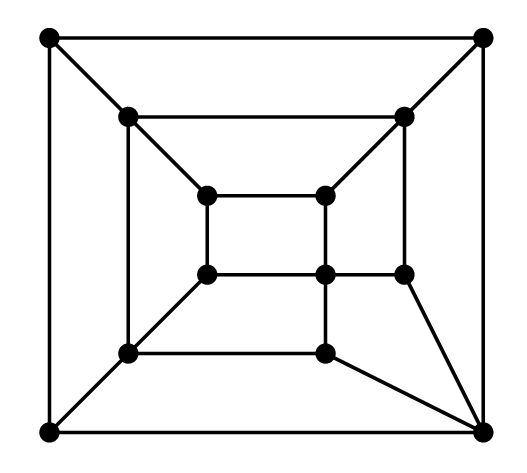
In the case of cubical $3$-polytopes, the derivative complex may consist of one or many $1$-spheres. For example, for the $3$-cube it consists of three $1$-spheres, while for the “cubical octahedron” $O_{8}$ displayed in Figure 2 the dual manifold is a single immersed $S^{1}$ (with $8$ double points).

In the case of $4$-polytopes, the dual manifolds are surfaces (compact $2$-manifolds without boundary). As an example, we here display a Schlegel diagram of a “neighborly cubical” $4$-polytope (with the graph of the $5$-cube), with $f$-vector $(32,80,96,48)$.

According to Joswig & Ziegler [21] this may be constructed as

Here the dual manifolds are four embedded cubical $2$-spheres $S^{2}$ with $f$-vector $(16,28,14)$ — of two different combinatorial types — and one embedded torus $T$ with $f$-vector $(16,32,16)$.

Let $P$ be a cubical $d$-polytope $(d\geq 3$). The immersed dual manifolds in its boundary cross the edges of the polytope transversally.

Thus we find that orientability of the dual manifolds is equivalent to the possibility to give consistent edge orientations to the edges of the $P$, that is, in each $2$-face of $P$ opposite edges should get parallel (rather than antiparallel) orientations; compare Hetyei [17]. Figure 4 shows such an edge orientation for a cubical $3$-polytope (whose derivative complex consists of three circles, so it has $8$ consistent edge orientations in total).

One can attempt to obtain such edge orientations by moving to from edge to edge across $2$-faces. The obstruction to this arises if on a path moving from edge to edge across quadrilateral $2$-faces we return to an already visited edge, with reversed orientation, that is, if we close a cubical Möbius strip with parallel inner edges, as displayed in the figure. (Such an immersion is not necessarily embedded, that is, some $2$-face may be used twice for the Möbius strip.)

The emphasis in this paper is on cubical convex $d$-polytopes. In the more general setting of cubical PL ($d-1$)-spheres, one has more flexible tools available. In this setting, Babson & Chan [3] proved that “all PL codimension $1$ normal crossing immersions appear.” The following sketch is meant to explain the Babson-Chan theorem geometrically (it is presented in a combinatorial framework and terminology in [3]), and to briefly indicate which parts of their construction are available in the polytope world.

Construction 1: Babson-Chan [3]

• • Input:

    A normal crossing immersion $j:\mathcal{M}^{d-2}\rightarrow\mathcal{S}^{d-1}$ of a triangulated PL manifold $\mathcal{M}^{d-2}$ of dimension $d-2$ into a PL simplicial ($d-1$)-sphere.

  • Output:

    A cubical PL ($d-1$)-sphere with a dual manifold immersion PL-equivalent to $j$.

  • (1)

    Perform a barycentric subdivision on $\mathcal{M}^{d-2}$ and $\mathcal{S}^{d-1}$.

    

      

    (Here each $i$-simplex is replaced by $(i+1)!$ new $i$-simplices, which is an even number for $i>0$. This step is done only to ensure parity conditions on the $f$-vector, especially that the number of facets of the final cubical sphere is congruent to the Euler characteristic of $\mathcal{M}^{d-2}$. Barycentric subdivisions are easily performed in the polytopal category as well, see Ewald & Shephard [11].)

  • (2)

    Perform a “cubical barycentric subdivision” on $\mathcal{M}^{d-2}$ and $\mathcal{S}^{d-1}$.

    

    (This is the standard tool for passage from a simplicial complex to a PL-homeomorphic cubical complex; here every $i$-simplex is subdivided into $i+1$ different $i$-cubes. Such cubations can be performed in the polytopal category according to Shephard [29]: If the starting triangulation of $\mathcal{S}^{d-1}$ was polytopal, the resulting cubation will be polytopal as well.)

  • (3)

    “Thicken” the cubical ($d-1$)-sphere along the immersed ($d-2$)-manifold, to obtain the cubical ($d-1$)-sphere $BC(\mathcal{S}^{d-1},j(\mathcal{M}^{d-2}))$.

    (In this step, every ($d-1-i$)-cube in the $i$-fold multiple point locus results in a new $(d-1)$-cube. The original immersed manifold, in its cubified subdivided version, now appears as a dual manifold in the newly resulting $(d-1)$-cubes. This last step is the one that seems hard to perform for polytopes in any non-trivial instance.)

  

In the following, the primary object we deal with is a regular ball: a regular polytopal subdivision $\mathcal{B}$ of a convex polytope $P=|\mathcal{B}|$.

In this definition, subdivisions of the boundary are allowed, that is, we do not necessarily require that the faces of $P=|\mathcal{B}|$ are themselves faces in $\mathcal{B}$.

In the sequel we focus on regular cubical balls. Only in some cases we consider regular non-cubical balls.

When constructing cubical complexes we often deal with regular cubical balls which are equipped with a lifting function. A lifted $d$-ball is a pair $(\mathcal{B},h)$ consisting of a regular $d$-ball $\mathcal{B}$ and a lifting function $h$ of $\mathcal{B}$. The lifted boundary of a lifted ball $(\mathcal{B},h)$ is the pair $(\partial\mathcal{B},h|_{\partial\mathcal{B}})$.

If $(\mathcal{B},h)$ is a lifted $d$-ball in ${\mathbb{R}}^{d^{\prime}}$ then $\operatorname{lift}(\mathcal{B},h)$ denotes the copy of $\mathcal{B}$ in ${\mathbb{R}}^{d^{\prime}+1}$ with vertices $(\boldsymbol{v},h(\boldsymbol{v}))\in{\mathbb{R}}^{d^{\prime}+1}$, $\boldsymbol{v}\in\verticesOP({\mathcal{B}})$. (In the sequel we sometimes do not distinguish between these two interpretations of a lifted ball.) We rely on Figure 10 for the illustration of this correspondence.

Often a lifted ball $(\mathcal{B},\psi)$ is constructed as follows: Let $P$ be a $d$-polytope (in ${\mathbb{R}}^{d}$) and $Q\subset{\mathbb{R}}^{d+1}$ a $(d+1)$-polytope such that $\pi(Q)=P$. Then the complex $\mathcal{B}^{\prime}$ given as the set of upper faces of $Q$ determines a lifted polytopal subdivision $(\mathcal{B},\psi)$ of $P$ (where $\mathcal{B}:=\pi(\mathcal{B}^{\prime})$ and $\psi$ is determined the vertex heights $\gamma(\boldsymbol{v})$, $\boldsymbol{v}\in\verticesOP({\mathcal{B}^{\prime}})$). Hence $\operatorname{lift}(\mathcal{B},\psi)$ equals $\mathcal{B}^{\prime}$. Compare again Figure 10.

The lifted boundary subdivision of a $d$-polytope $P$ is a pair $(\mathcal{S}^{d-1},\psi)$ consisting of a polytopal subdivision $\mathcal{S}^{d-1}$ of the boundary of $P$ and a piece-wise linear function $\psi:|\partial{P}|\rightarrow{\mathbb{R}}$ such that for each facet $F$ of $P$ the restriction of $\psi$ to $F$ is a lifting function of the induced subdivision $\mathcal{S}^{d-1}\cap F$ of $F$.

Often regular cubical balls are constructed from other regular balls. The following “patching lemma”, which appears frequently in the construction of regular subdivisions (see [22, Cor. 1.12] or [8, Lemma 3.2.2]) is a basic tool for this.

As a consequence, the prism $\operatorname{prism}(\mathcal{C})$ over a cubical $d$-complex $\mathcal{C}$ yields a cubical $(d+1)$-dimensional complex. Furthermore, the prism over a regular cubical ball $\mathcal{B}$ yields a regular cubical $(d+1)$-ball.

For integers $\ell_{1},\ldots,\ell_{d}\geq 1$, the pile of cubes $P_{d}(\ell_{1},\ldots,\ell_{d})$ is the cubical $d$-ball formed by all unit cubes with integer vertices in the $d$-polytope $P:=[0,\ell_{1}]\times\ldots\times[0,\ell_{d}]$, that is, the cubical $d$-ball formed by the set of all $d$-cubes

for integers $0\leq k_{i}<\ell_{i}$ together with their faces [33, Sect. 5.1].

The pile of cubes $P_{d}(\ell_{1},\ldots,\ell_{d})$ is a product of $1$-dimensional subdivisions, which are regular. Hence the product lemma implies that $P_{d}(\ell_{1},\ldots,\ell_{d})$ is a regular cubical subdivision of the $d$-polytope $P$.

The following construction yields a “connector” polytope that may be used to attach cubical $4$-polytopes resp. regular cubical $4$-balls without the requirement that the attaching facets are projectively equivalent.

While there appears to be no simple construction that would produce a cubical ($d+1$)-polytope from a given cubical $d$-polytope, we do have a simple prism construction that produces regular cubical ($d+1$)-balls from regular cubical $d$-balls.

Construction 2: Lifted prism

• Input:	A lifted cubical $d$-ball $(\mathcal{B},h)$.
  Output:	A lifted cubical ($d+1$)-ball $\mathop{\textsc{LiftedPrism}}(\mathcal{B},h)$
  	which is combinatorially isomorphic to the prism over $\mathcal{B}$.

  We may assume that the convex lifting function $h$ defined on $P:=|\mathcal{B}|$ is strictly positive. Then the lifted facets of $\mathop{\textsc{LiftedPrism}}(\mathcal{B},h)$ may be taken to be the sets

  $$\widetilde{F}\ \ :=\ \ \{(\boldsymbol{x},t,h(\boldsymbol{x})):\boldsymbol{x}\in F,\ -h(\boldsymbol{x})\leq t\leq+h(\boldsymbol{x})\},\qquad F\in\operatorname{fac}({\mathcal{B}}).\vskip-19.91692pt$$

If $\mathcal{B}$ does not subdivide the boundary of $P$, then $\mathop{\textsc{LiftedPrism}}(\mathcal{B},h)$ does not subdivide the boundary of $|\mathop{\textsc{LiftedPrism}}(\mathcal{B},h)|$. In this case $\widehat{P}:=|\mathop{\textsc{LiftedPrism}}(\mathcal{B},h)|$ is a cubical $(d+1)$-polytope whose boundary complex is combinatorially isomorphic to the boundary of the prism over $\mathcal{B}$. The $f$-vector of $\widehat{P}$ is then given by

Figure 11 shows the lifted prism over a lifted cubical $2$-ball.

Another modification of this construction is to take two different lifted cubical balls $(\mathcal{B}_{1},h_{1})$ and $(\mathcal{B}_{2},h_{2})$ with the same lifted boundary complex (that is, $\partial\mathcal{B}_{1}=\partial\mathcal{B}_{2}$ with $h_{1}(\boldsymbol{x})=h_{2}(\boldsymbol{x})$ for all $\boldsymbol{x}\in\partial\mathcal{B}_{1}=\partial\mathcal{B}_{2}$) as input. In this case the outcome is a cubical ($d+1$)-polytope which may not even have a cubification.

Construction 3: Lifted prism over two balls

• • Input:

    Two lifted cubical $d$-balls $(\mathcal{B}_{1},h_{1})$ and $(\mathcal{B}_{2},h_{2})$
    with the same lifted boundary.

  • Output:

    A cubical ($d+1$)-polytope $\mathop{\textsc{LiftedPrism}}((\mathcal{B}_{1},h_{1}),(\mathcal{B}_{2},h_{2}))$
    with lifted copies of $\mathcal{B}_{1}$ and $\mathcal{B}_{1}$ in its boundary.

  If both balls do not subdivide their boundaries, we set $\mathcal{B}^{\prime}_{k}:=\mathcal{B}_{k}$ and $h^{\prime}_{k}:=h_{k}$ for $k\in\{1,2\}$. Otherwise we apply the construction of the proof of Lemma 3.2 simultaneously to both lifted cubical balls $(\mathcal{B}_{1},h_{1})$ and $(\mathcal{B}_{2},h_{2})$ to obtain two lifted cubical $d$-balls $(\mathcal{B}^{\prime}_{1},h^{\prime}_{1})$ and $(\mathcal{B}^{\prime}_{2},h^{\prime}_{2})$ with the same support $Q=|\mathcal{B}_{1}|=|\mathcal{B}_{2}|$ which do not subdivide the boundary of $Q$.

  We can assume that $h^{\prime}_{1},h^{\prime}_{2}$ are strictly positive. Then $\widehat{Q}:=\mathop{\textsc{LiftedPrism}}((\mathcal{B}_{1},h_{1}),(\mathcal{B}_{2},h_{2}))$ is defined as the convex hull of the points in

  $$\{(\boldsymbol{x},+h^{\prime}_{1}(\boldsymbol{x})):\boldsymbol{x}\in|\mathcal{B}^{\prime}_{1}|\}\ \cup\ \{(\boldsymbol{x},-h^{\prime}_{2}(\boldsymbol{x})):\boldsymbol{x}\in|\mathcal{B}^{\prime}_{2}|\},$$

  Since $\mathcal{B}^{\prime}_{1}$ and $\mathcal{B}^{\prime}_{2}$ both do not subdivide their boundaries, each of their proper faces yields a face of $\widehat{Q}$. Furthermore, $\widehat{Q}$ is a cubical $(d+1)$-polytope whose $f$-vector is given by

  $$f_{k}(\widehat{Q})\ \ =\ \ \begin{cases}f_{0}(\mathcal{B}_{1})+f_{0}(\mathcal{B}_{2})&\textrm{ for }k=0,\\ f_{k}(\mathcal{B}_{1})+f_{k}(\mathcal{B}_{2})+f_{k-1}(\partial\mathcal{B}_{1})&\textrm{ for }0<k\leq d.\end{cases}$$

  See Figure 12.

The following is a projective variant of the prism construction, applied to a $d$-polytope $P$.

Construction 4: Schlegel cap

• • Input:

    An almost cubical $d$-polytope $(P,F_{0})$

  • Output:

    A regular cubical $d$-ball $\mathop{\textsc{SchlegelCap}}(P,F_{0})$, with $P\subset|\mathop{\textsc{SchlegelCap}}(P,F_{0})|$ which is combinatorially isomorphic to the prism over $\mathop{\textsc{Schlegel}}(P,F)$.

  The construction of the Schlegel cap depends on two further pieces of input data, namely on a point $\boldsymbol{x}_{0}\in{\mathbb{R}}^{d}$ beyond $F_{0}$ (and beneath all other facets of $P$; cf. [15, Sect. 5.2]) and on a hyperplane $H$ that separates $\boldsymbol{x}_{0}$ from $P$. In terms of projective transformations it is obtained as follows:

  • (1)

    Apply a projective transformation that moves $\boldsymbol{x}_{0}$ to infinity while fixing $H$ pointwise. This transformation moves the Schlegel complex $\mathcal{C}({\partial P}){\setminus}\{F_{0}\}$ to a new cubical complex $\mathcal{E}$.

  • (2)

    Reflect the image $\mathcal{E}$ of the Schlegel complex in $H$, and call its reflected copy $\mathcal{E}^{\prime}$.

  • (3)

    Build the polytope bounded by $\mathcal{E}$ and $\mathcal{E}^{\prime}$.

  • (4)

    Reverse the projective transformation of (1).

  

      

  An alternative description, avoiding projective transformations, is as follows:

  • (1)

    For each point $\boldsymbol{x}$ in the Schlegel complex $\mathcal{C}({\partial P}){\setminus}\{F_{0}\}$ let $\bar{\boldsymbol{x}}$ be the intersection point of $H$ and the segment $[\boldsymbol{x}_{0},\boldsymbol{x}]$, and let $\boldsymbol{x}^{\prime}$ be the point on the segment $[\boldsymbol{x}_{0},\boldsymbol{x}]$ such that $[\boldsymbol{x}_{0},\bar{\boldsymbol{x}};\boldsymbol{x}^{\prime},\boldsymbol{x}]$ form a harmonic quadruple (cross ratio $-1$).

    That is, if $\vec{\boldsymbol{v}}$ is a direction vector such that $\boldsymbol{x}=\boldsymbol{x}_{0}+t\vec{\boldsymbol{v}}$ for some $t>1$ denotes the difference $\boldsymbol{x}-\boldsymbol{x}_{0}$, while $\bar{\boldsymbol{x}}=\boldsymbol{x}_{0}+\vec{\boldsymbol{v}}$ lies on $H$, then $\boldsymbol{x}^{\prime}=\boldsymbol{x}_{0}+\frac{t}{2t-1}\vec{\boldsymbol{v}}$.

  • (2)

    For each face $G$ of the Schlegel complex, $G^{\prime}:=\{\boldsymbol{x}^{\prime}:\boldsymbol{x}\in G\}$ is the “projectively reflected” copy of $G$ on the other side of $H$.

  • (3)

    The Schlegel cap $\mathop{\textsc{SchlegelCap}}(P,F_{0})$ is the regular polytopal ball with faces $G$, $G^{\prime}$ and $\mathop{\operatorname{conv}}(G\cup G^{\prime})$ for faces $G$ in the Schlegel complex.

  

Yamakawa & Shimada [32] have introduced an interesting polytopal construction in dimension $3$ called the Hexhoop template; see Figure 18.

Their construction takes as input a $3$-polytope $P$ that is affinely isomorphic to a regular $3$-cube, a hyperplane $H$ and a cubical subdivision $\mathcal{S}$ of the boundary complex of $P$ such that $\mathcal{S}$ is symmetric with respect to $H$ and $H$ intersects no facet of $\mathcal{S}$ in its relative interior. For such a cubical PL $2$-sphere $\mathcal{S}$ the Hexhoop template produces a cubification. A $2$-dimensional version is shown in Figure 19.

In the following we present a generalized regular Hexhoop construction. It is a generalization of the Hexhoop template in several directions: Our approach admits arbitrary geometries, works in any dimension, and yields regular cubifications with “prescribed heights on the boundary” (with a symmetry requirement and with the requirement that the intersection of the symmetry hyperplane and the boundary subdivision is a subcomplex of the boundary subdivision).
Figure 20 displays a $2$-dimensional cubification (of a boundary subdivision $\mathcal{S}$ of a $2$-polytope such that $\mathcal{S}$ is symmetric with respect to a hyperplane $H$) obtained by our construction.

Not only do we get a cubification, but we may also derive a symmetric lifting function for the cubification that may be quite arbitrarily prescribed on the boundary. The input of our construction is a lifted cubical boundary subdivision $(\mathcal{S}^{d-1},\psi)$ of a $d$-polytope $P$, such that both $P$ and $(\mathcal{S}^{d-1},\psi)$ are symmetric with respect to a hyperplane $H$.

Our approach goes roughly as follows.

• (1)

  We first produce a $(d+1)$-polytope $T$ that is a symmetric tent (defined in Section 6.3) over the given lifted boundary subdivision $(\mathcal{S},\psi)$ of the input $d$-polytope $P$. Such a tent is the convex hull of all ‘lifted vertices’ $(\boldsymbol{v},\psi(\boldsymbol{v}))\in{\mathbb{R}}^{d+1}$, $\boldsymbol{v}\in\verticesOP({\mathcal{S}})$, and of two apex points $\boldsymbol{p}_{L},\boldsymbol{p}_{R}$; compare Figure 22.

  

• (2)

  Truncate $T$ by a hyperplane $H^{\prime}$ parallel to $\affOP(P)={\mathbb{R}}^{d}\subset{\mathbb{R}}^{d}\times\{0\}$ that separates the lifted points from the apex points, and remove the upper part.

• (3)

  Add the polytope $R:=\coneOP(\boldsymbol{p}_{L},Q)\cap\coneOP(\boldsymbol{p}_{R},Q)\cap H^{\prime}_{+}$, where $H^{\prime}_{+}$ is the halfspace with respect to $H$ that contains $\boldsymbol{p}_{L}$ and $\boldsymbol{p}_{R}$. Compare Figure 23.

• (4)

  Project the upper boundary complex of the resulting polytope to ${\mathbb{R}}^{d}$.

The figures in this section illustrate the generalized regular Hexhoop construction for the $2$-dimensional input polytope of Figure 21; the generalized Hexhoop construction for $d=2$ yields $2$-dimensional complexes in ${\mathbb{R}}^{3}$. The extension to higher dimensions is immediate, and the case $d=3$ is crucial for us (see Section 7). It is, however, also harder to visualize: A $3$-dimensional generalized regular Hexhoop cubification is shown in Figure 29.

Let $P$ be a $d$-polytope that is symmetric with respect to a hyperplane $H$ in ${\mathbb{R}}^{d}$. Choose a positive halfspace $H_{+}$ with respect to $H$. Let $(\mathcal{S},\psi)$ be a lifted boundary subdivision of $P$ such that $\mathcal{S}\cap H$ is a subcomplex of $\mathcal{S}$. Define $\widetilde{H}:=H+{\mathbb{R}}\boldsymbol{e}_{d+1}$, which is a symmetry hyperplane for $P\subset{\mathbb{R}}^{d+1}$. The positive halfspace of $\widetilde{H}\subset{\mathbb{R}}^{d+1}$ will be denoted by $\widetilde{H}_{+}$.

The symmetric tent over $(\mathcal{S},\psi)$ is the lifted polytopal subdivision $(\mathcal{T},\phi)$ of $P$ given by the upper faces of the polytope

if $\boldsymbol{p}_{L},\boldsymbol{p}_{R}\in{\mathbb{R}}^{d+1}$ are two apex points in ${\mathbb{R}}^{d+1}$ that are symmetric with respect to the hyperplane $\widetilde{H}$, and the upper facets of $T$ are

• •

  pyramids with apex point $\boldsymbol{p}_{L}$ over facets $F$ of $\operatorname{lift}(\mathcal{S},\psi)$ such that $\pi(F)\subset H_{+}$,

• •

  pyramids with apex point $\boldsymbol{p}_{R}$ over facets $F$ of $\operatorname{lift}(\mathcal{S},\psi)$ such that $\pi(F)\subset H_{-}$, and

• •

  $2$-fold pyramids with apex points $\boldsymbol{p}_{L},\boldsymbol{p}_{R}$ over ridges $R$ of $\operatorname{lift}(\mathcal{S},\psi)$ with $\pi(R)\subset H$.

(This requires that $\boldsymbol{p}_{L}\not\in\affOP(P)$ and $\pi(\boldsymbol{p}_{L})\in\relintOP(P\cap H_{+})$.)

This can be shown for instance by using the Patching Lemma (Lemma 3.3).

In this section we specify our generalization of the Hexhoop template and prove the following existence statement for cubifications.

The proof relies on the following construction.

Construction 5: Generalized regular Hexhoop

• Input:

  • $P$

    a convex $d$-polytope $P$ in ${\mathbb{R}}^{d}$.

  • $(\mathcal{S}^{d-1},\psi)$

    a lifted cubical boundary subdivision of $P$.

  • $H$

    a hyperplane in ${\mathbb{R}}^{d}$ such that

    • *

      $P$ and $(\mathcal{S}^{d-1},\psi)$ are symmetric with respect to $H$, and

    • *

      $\mathcal{S}^{d-1}\cap H$ is a subcomplex of $\mathcal{S}^{d-1}$.

  Output:

  • $(\mathcal{B}^{d},\phi)$

    a symmetric lifted cubification of $(\mathcal{S}^{d-1},\psi)$ given by a cubical $d$-ball $\mathcal{C}^{\prime}$ in ${\mathbb{R}}^{d+1}$.

  • (1)

    Choose a positive halfspace $H_{+}$ with respect to $H$, and a point $\boldsymbol{q}_{L}\in\relintOP(P\cap H_{+})$. Define $\boldsymbol{q}_{R}:=\boldsymbol{p}_{L}^{M}$, where the upper index ^M denotes the mirrored copy with respect to $\widetilde{H}=H+{\mathbb{R}}\boldsymbol{e}_{d+1}$.

    By Lemma 6.1 there is a height $h>0$ such that

    $$T:=\mathop{\operatorname{conv}}\{\operatorname{lift}(\mathcal{S}^{d-1},\psi),\boldsymbol{p}_{L},\boldsymbol{p}_{R}\}$$

    with $\boldsymbol{p}_{L}:=(\boldsymbol{q}_{L},h)$ and $\boldsymbol{p}_{R}:=(\boldsymbol{q}_{R},h)$ forms a symmetric tent over $(\mathcal{S}^{d-1},\psi)$.

  • (2)

    Choose a hyperplane $H^{\prime}$ parallel to $\affOP(P)\subset{\mathbb{R}}^{d}$ that separates $\{\boldsymbol{p}_{L},\boldsymbol{p}_{R}\}$ and $\operatorname{lift}(\mathcal{S}^{d-1},\psi)$. Let $H^{\prime}_{+}$ be the halfspace with respect to $H^{\prime}$ that contains $\boldsymbol{p}_{L}$ and $\boldsymbol{p}_{R}$.

    

  • (3)

    Define the “lower half” of the tent $T$ as

    $$T_{-}\ :=\ T\cap H^{\prime}_{-},$$

    whose “top facet” is the convex $d$-polytope $Q:=T\cap H^{\prime}$.

    

  • (4)

    Define the two $d$-polytopes

    	$\displaystyle Q_{L}$	$\displaystyle:=$	$\displaystyle\mathop{\operatorname{conv}}{\left\{{\boldsymbol{v}\in\verticesOP({Q})}\,:\,{\boldsymbol{v}\in H_{+}}\right\}},$
    	$\displaystyle Q_{R}$	$\displaystyle:=$	$\displaystyle\mathop{\operatorname{conv}}{\left\{{\boldsymbol{v}\in\verticesOP({Q})}\,:\,{\boldsymbol{v}\in H_{-}}\right\}}.$

    Let $F_{L}:=H^{\prime}\cap\convOP(\boldsymbol{p}_{L},P\cap H)$, the unique facet of $Q_{L}$ that is not a facet of $Q$.

    

  • (5)

    Construct the polytope

    $$R\ \ :=\ \ \coneOP(\boldsymbol{p}_{L},Q)\ \cap\ \coneOP(\boldsymbol{p}_{R},Q)\ \cap\ H^{\prime}_{+}.$$

    

  The complex $\mathcal{C}^{\prime}$ in question is given by the upper facets of the $(d+1)$-polytope

  $$U\ :=\ T_{-}\cup R.$$

References

- [1] P. M. Akhmetev, An elementary proof of the Freedman immersion theorem, St. Petersburg Math. J. 7 (1996), 749–754.
- [2] F. Apéry, Models of the Real Projective Plane, Vieweg, Braunschweig 1987.
- [3] E. K. Babson and C. Chan, Counting faces for cubical spheres modulo two, Discrete Math. 212 (2000), 169–183.
- [4] T. F. Banchoff, Triple points and surgery of immersed surfaces, Proc. Amer. Math. Soc. 46 (1974), 407–413.
- [5] M. W. Bern, D. Eppstein, and J. G. Erickson, Flipping cubical meshes, Engineering with Computers 18 (2002), 173–187.
- [6] G. Blind and R. Blind, Gaps in the numbers of vertices of cubical polytopes, I, Discrete Comput. Geometry 11 (1994), 351–356.
- [7] W. Boy, Über die Curvatura integra und die Topologie geschlossener Flächen, Mathematische Annalen 57 (1903), 151–184.
- [8] W. Bruns, J. Gubeladze, and N. V. Trung, Normal polytopes, triangulations, and Koszul algebras, J. Reine Angew. Math. 485 (1997), 123–160.
- [9] N. Dolbilin, M. Shtan’ko, and M. Shtogrin, Cubic manifolds in lattices, Russ. Acad. Sci. Izv. Math. 44 (1995), 301–313.
- [10] D. Eppstein, Linear complexity hexahedral mesh generation, Comput. Geom. 12 (1999), 3–16.
- [11] G. Ewald and G. C. Shephard, Stellar subdivisions of boundary complexes of convex polytopes, Mathematische Annalen 210 (1974), 7–16.
- [12] G. Francis, J. M. Sullivan, and C. Hartman, Computing sphere eversions, in “Mathematical Visualization (Berlin, 1997)”, Springer, Berlin 1998, pp. 237–255.
- [13] M. Freedman, Quadruple points of -manifolds in , Commentarii Math. Helv. 53 (1978), 385–394.
- [14] E. Gawrilow and M. Joswig, polymake: a framework for analyzing convex polytopes. TU Berlin, 1997–2003, www.math.tu-berlin.de/polymake.
- [15] B. Grünbaum, Convex Polytopes, Graduate Texts in Math. 221, Springer, New York 2003. Second ed. by V. Kaibel, V. Klee and G.M. Ziegler (original edition: Interscience, London 1967).
- [16] F. Heckenbach, Die Möbiusfunktion und Homologien auf partiell geordneten Mengen. Diplomarbeit Erlangen, 1997. (Computer program homology, www.mi.uni-erlangen.de/~heckenb/).
- [17] G. Hetyei, On the Stanley ring of a cubical complex, Discrete Comput. Geometry 14 (1995), 305–330.
- [18] D. Hilbert and S. Cohn-Vossen, Anschauliche Geometrie. Springer, Berlin 1932; 2nd edition 1996. English translation: Geometry and the Imagination, Chelsea, New York 1952.
- [19] J. F. P. Hudson, Piecewise Linear Topology, W.A. Benjamin, New York 1969.
- [20] W. Jockusch, The lower and upper bound problems for cubical polytopes, Discrete Comput. Geometry 9 (1993), 159–163.
- [21] M. Joswig and G. M. Ziegler, Neighborly cubical polytopes, Discrete Comput. Geometry 24 (2000), 325–344.
- [22] G. R. Kempf, F. F. Knudsen, D. Mumford, and B. Saint-Donat, Toroidal Embeddings I, Lecture Notes in Mathematics 339, Springer, Heidelberg 1973.
- [23] S. A. Mitchell, A characterization of the quadrilateral meshes of a surface which admit a compatible hexahedral mesh of the enclosed volume, in Proc. 13th Symp. Theoretical Aspects of Computer Science (STACS’96), Lecture Notes in Computer Science 1046, Springer, Heidelberg 1996, pp. 465–476.
- [24] J. R. Munkres, Elements of Algebraic Topology, Addison-Wesley, Menlo Park, CA 1984.
- [25] J.-P. Petit, Das Topologikon, Vieweg, Braunschweig 1995.
- [26] K. Polthier, S. Khadem, E. Preuß, and U. Reitebuch, JavaView visualization software, TU Berlin 1999–2002. www.javaview.de.
- [27] C. Rourke and B. Sanderson, Introduction to Piecewise-Linear Topology, Springer, Berlin 1972. Revised printing (Springer Study Edition) 1982.
- [28] A. Schwartz, Constructions of Cubical Polytopes, PhD thesis, TU Berlin, 2003.
- [29] G. C. Shephard, Approximations by polytopes with projectively regular facets, Mathematika 13 (1966), 189–195.
- [30] S. Smale, A classification of immersions of the two-sphere, Trans. Amer. Math. Soc. 90 (1958), 281–290.
- [31]
W. Thurston, Hexahedral decomposition of polyhedra.
Posting to sci.math, 1993.
www.ics.uci.edu/~eppstein/gina/Thurston-hexahedra.html. - [32] S. Yamakawa and K. Shimada, Hexhoop: Modular templates for converting a hex-dominant mesh to an all-hex mesh, in Proc. 10th Int. Meshing Roundtable, Sandia Nat. Lab., October 2001, pp. 235-246; Engineering with Computers 18 (2002), 211–228.
- [33] G. M. Ziegler, Lectures on Polytopes, Graduate Texts in Mathematics 152, Springer, New York 1995. Revised edition, 1998.