Root games on Grassmannians
Abstract
We recall the root game, introduced in [P], which gives a fairly powerful sufficient condition for non-vanishing of Schubert calculus on a generalised flag manifold . We show that it gives a necessary and sufficient rule for non-vanishing of Schubert calculus on Grassmannians. In particular, a Littlewood-Richardson number is non-zero if and only if it is possible to win the corresponding root game. More generally, the rule can be used to determine whether or not a product of several Schubert classes on is non-zero in a manifestly symmetric way. Finally, we give a geometric interpretation of root games for Grassmannian Schubert problems.
1 Prior work
In [P] we introduced the root game, a combinatorial game which can often determine whether or not a given Schubert structure constant is zero in the cohomology ring of a generalised flag manifold . Our goal in this paper is to strengthen our earlier results in the case where the group is and the Schubert classes are pulled back from a Grassmannian. We begin by recalling the root game for Schubert intersection numbers on the (ordinary) flag manifold . Apart from the root game, most of the relevant background material for this paper can be found in [F1, FG].
Let . Let and denote the Borel subgroups of upper and lower triangular matrices respectively, and the standard maximal torus, consisting of invertible diagonal matrices.
Recall that for each element of the symmetric group , there is a corresponding -fixed point on the flag manifold (here we view as an element of via the standard representation of ), and an associated Schubert variety . We denote its cohomology class in by .
Our convention will be to write all permutations in one line notation
If denotes the identity element, and is the long word, then the Schubert class is the identity element in , and is the class of a point. In general is a class of degree , where denotes the length of .
For , the Schubert intersection number
| (1) |
is always a non-negative integer. The root game attempts to determine whether this number is strictly positive.
The game is played on a set of squares . In our diagrams, we will arrange the squares in an array, where is the row index and is the column index. In each square we allow tokens to appear. Each token has a label , and no square may ever contain two tokens with the same label. A token labelled is called a -token, and we write if a -token appears in square .
A position in the game is specified by two pieces of data:
- •
The configuration of the tokens. Formally this is a map from to subsets of , and our notation is shorthand for ; however, in this paper we will wish to think of each token as a physical object which can be moved from square to square.
- •
A partition of the set of squares . Each is called a region.
The initial position of the game is as follows: there is a single region , and for , a -token appears in square if and only if .
From the initial position we move the tokens in the manner prescribed in the next paragraph. However, before each move we have the option of splitting regions into multiple regions. We define an ideal subset of the squares to be a set with the property that if , and then . Given an ideal subset of the squares we can break up a region into two regions: and . We call this splitting along , and we may repeat the process as many times as desired.
A move is specified by a region , a token label and a pair with . After choosing these data, we move tokens as follows:
- •
For every with , if and are both in and a -token appears in but not in , we move the -token from to ;
- •
For every with , if and are both in and a -token appears in but not in , we move the -token from to .
More succinctly put, within the region we move -tokens horizontally from column to column and vertically from row to row , wherever possible. See Figure 1.
In the play of the game we may make any sequence of moves in any order. The game is won when there is exactly one token in each square.

Remark 1.1.
It turns out to be advantageous to split along an ideal subset if and only if the total number of tokens in all squares in equals . We call the process of finding all such and splitting along them splitting maximally. Although in this paper we won’t take full advantage of this fact by splitting maximally before every move, we will never even consider the possibility of splitting along if this condition is not met.
The main result that we shall need is the following.
Theorem 1 ([P]).
If the game for can be won, then
In general we do not know if the converse of Theorem 1 is true. When , the Schubert intersection numbers (1) are structure constants for the ring , and in this case the converse has been confirmed for . It would certainly be remarkable if it were true in general.
We can also use the game to study the cohomology rings of partial flag manifolds by pulling back cohomology classes to the full flag manifold. In this paper, we investigate this in some detail in the case of the Grassmannian. Our main result is a version of the converse of Theorem 1 for Grassmannian Schubert calculus.
When and the classes come from a Grassmannian, the intersection numbers (1) are Littlewood-Richardson numbers. These numbers are also important in representation theory and in the theory of symmetric functions—they are the structure constants for the representation ring of , and for the ring of symmetric functions in the Schur basis. As such, they are well studied, and there are a number of combinatorial rules, and geometric rules (e.g. [C, V]) known for computing these numbers.
Remark 1.2.
An interesting and pleasant feature of root games is that the rules naturally extend to any number Schubert classes in a way which is manifestly symmetrical in these inputs: it is immediately clear from the definitions that reordering the input permutations does not affect whether or not the game can be won. This property is not generally shared by other combinatorial or geometric rules for Littlewood-Richardson numbers. Most of the known rules have no manifest symmetry. Knutson-Tao puzzles [KTW] are perhaps the most manifestly symmetrical Littlewood-Richardson rule, having a -cyclic symmetry when , but this is lost when one attempts to generalise beyond beyond triple intersections.
The manifest symmetry of the root game on , descends to the Grassmannian case. In Section 2 we partially break this symmetry, but as we explain in Section 4, the full symmetry is easily restored. To our knowledge, the only other manifestly symmetrical rule in Grassmannian Schubert calculus is the Horn recursion (see the survey article [F2]), which, like the root game, does not explicitly compute Littlewood-Richardson numbers and is only for determining which Schubert intersection numbers are strictly positive.
2 Associating a game to a Grassmannian Schubert calculus problem
Definition 2.1.
A -string is a string where each . A -string is a -string , where exactly of the are equal to .
Schubert varieties in the Grassmannian are indexed by -strings. Fix a base flag
in . The Schubert variety corresponding to is
We denote its cohomology class in by . According to these conventions is the identity element in and is the class of a point.
Given a list of -strings , we will wish to study the Grassmannian Schubert intersection numbers
We do so by investigating an equivalent problem on a full flag manifold. The most obvious way to do this is to simply consider the product of the classes etc., under the natural map , as in Lemma 2.2 below. However, our purposes require that we do things in a somewhat less straightforward way.
Let be an integer, and let be a -string. Let denote the positions of the zeroes in , and denote the positions of the ones. We define three ways to associate a permutation to the -string :
From we produce a list of permutations, :
Proposition 2.1.
The proof is based on the following standard pullback calculations, whose proofs we omit.
Lemma 2.2.
Let be the map which forgets all but the -dimensional subspace of the flag. Then .
For a -string , let denote the string followed by ones, and let denote the string preceded by ones.
Lemma 2.3.
Let be the map . Then . If is not of the form for some -string then .
If is a partial flag variety and is a Schubert class, let denote the opposite Schubert class, i.e. the unique Schubert class such that . For example , and where is reversed.
If are Schubert classes then the statement that
| (2) |
is equivalent to the statement that
| (3) |
in the Schubert basis. We’ll call Equation (3) the -special version of Equation (2).
3 Non-vanishing for Grassmannians
Let be -strings (if , we’ll write instead of ). For any given , we associate permutations as before. Our goal in this section is to prove the following theorem.
Theorem 2.
Take suitably large ( will always suffice). The root game corresponding to can be won if and only if
Moreover, only moves involving tokens labelled are required.
Remark 3.1.
We shall first consider what happens in the case where .
Recall the correspondence between -strings and Young diagrams. Our Young diagrams will be in the French convention (the rows are left justified and increase in length as we move down). If is a -string , let denote the number of ones before the zero. We associate to the Young diagram whose row is , where we are allowing the possibility that some rows may have length .
If is a Young diagram, let denote the Young diagram obtained by adding squares to each row of including those rows which contain squares.
The initial positions of the -tokens are in the shape of the Young diagram . The initial positions of the -tokens are in the shape of a Young diagram . The squares that do not contain a -token are also in the shape of a Young diagram, which we’ll denote ; viewed upside down, is the complement to inside an rectangle. The lower left corner of each of the Young diagrams , , is in the square . See Figure 2 for an illustration of how these shapes are generated.
If , then it is a basic fact that (in fact this is a necessary and sufficient condition). Therefore, we may assume that no square contains both a -token and a -token. The squares which contain neither a -token nor a -token are empty squares—since is suitably large the -tokens are all to the left of these squares— and are in the shape of a skew-diagram .
At the outset of the game, some immediate splitting can occur. We split in such a way that each square containing a -token becomes a -square region of its own. (For some choices of it may be possible to split beyond this, but our argument is slightly simplified if we elect not to.) The remaining squares are those of , which form what we call the big region. The big region is the only region which is unsolved; naturally, therefore, this will be the region in which all moves take place.
It is worth taking a moment to note how tokens move within the big region. A priori, a move will cause some -tokens to move horizontally and others to move vertically. However, since the rows of the big region are indexed by , and the columns are indexed by the disjoint set , these cannot both happen. If then -tokens will move vertically from row to row . If then -tokens move horizontally from column to column . No tokens move if .

Definition 3.2 (Zelevinsky [Z]).
A picture between two (French) skew diagrams is a bijection between their boxes with the property that if box is weakly above and weakly right of box in one diagram, then the corresponding boxes and are in lexicographic order (i.e. precedes if or and ) in the other diagram.
Now is given by the Littlewood-Richardson coefficient , which can be described as the number of pictures between and [Z]. This is a reformulation of the Littlewood-Richardson rule [LR], closely related to the Remmel-Whitney formula [RW]. In particular, if this number is non-zero, there exists such a picture. We pick one, and denote by the map it defines from the squares of to the squares of . Note that all of these squares are in the big region of the game.
To show that the game can be won, we will give an algorithm— the Grassmannian root game algorithm (GRGA)—which uses to construct a sequence of moves that transports each -token to a square of .
Essential to the GRGA is the following numbering scheme. At each point in the game we associate a number—called the readiness number—to each unplaced -token (i.e. one which has not already reached its final destination) and each empty square of .
Definition 3.3.
At any point in the game, let be a -token whose initial square was and whose current square is . Let . Define the readiness number of both the token and the square to be the number . We say an empty square of or an unplaced -token is ready if its readiness number is . Tokens which have reached their final destination and non-empty squares are not considered ready.
The key properties of this numbering scheme are the following:
Lemma 3.1.
Initially, the readiness numbers of the unplaced -tokens are
- (a)
weakly increasing along each row, and
- (b)
weakly decreasing down each column;
in the readiness numbers of empty squares are
- (c)
weakly decreasing along each row, and
- (d)
weakly increasing down each column.
Moreover, the GRGA, described below, preserves all of these properties.
Proof.
(a) If and are squares of in the same row, and is right of , then by Definition 3.2 is lexicographically before . In particular, is weakly above , i.e. in the same row or a row above. Thus the readiness number of the token in the readiness number of the token in .
(b) If and are squares of , and is one square above , then again is lexicographically before . There are two cases. If is strictly above , then the readiness number of the token in the readiness number of the token in . Otherwise, and are in the same row in , with right of . But then by Definition 3.2, must be lexicographically before , which is a contradiction.
Statements (c) and (d) are proved similarly. That the GRGA preserves all these properties will be quite evident. ∎
Note that since the readiness number of the lower-leftmost token is at least , by Lemma 3.1 parts (a) and (b) the readiness numbers are initially all non-negative.
The Grassmannian root game algorithm (GRGA).
The algorithm assumes that the tokens are in the initial positions of the root game for (corresponding to with suitably large), that all -tokens have been split into their own one-square region, and that we have a picture between and . All moves take place in the big region.
- 1.
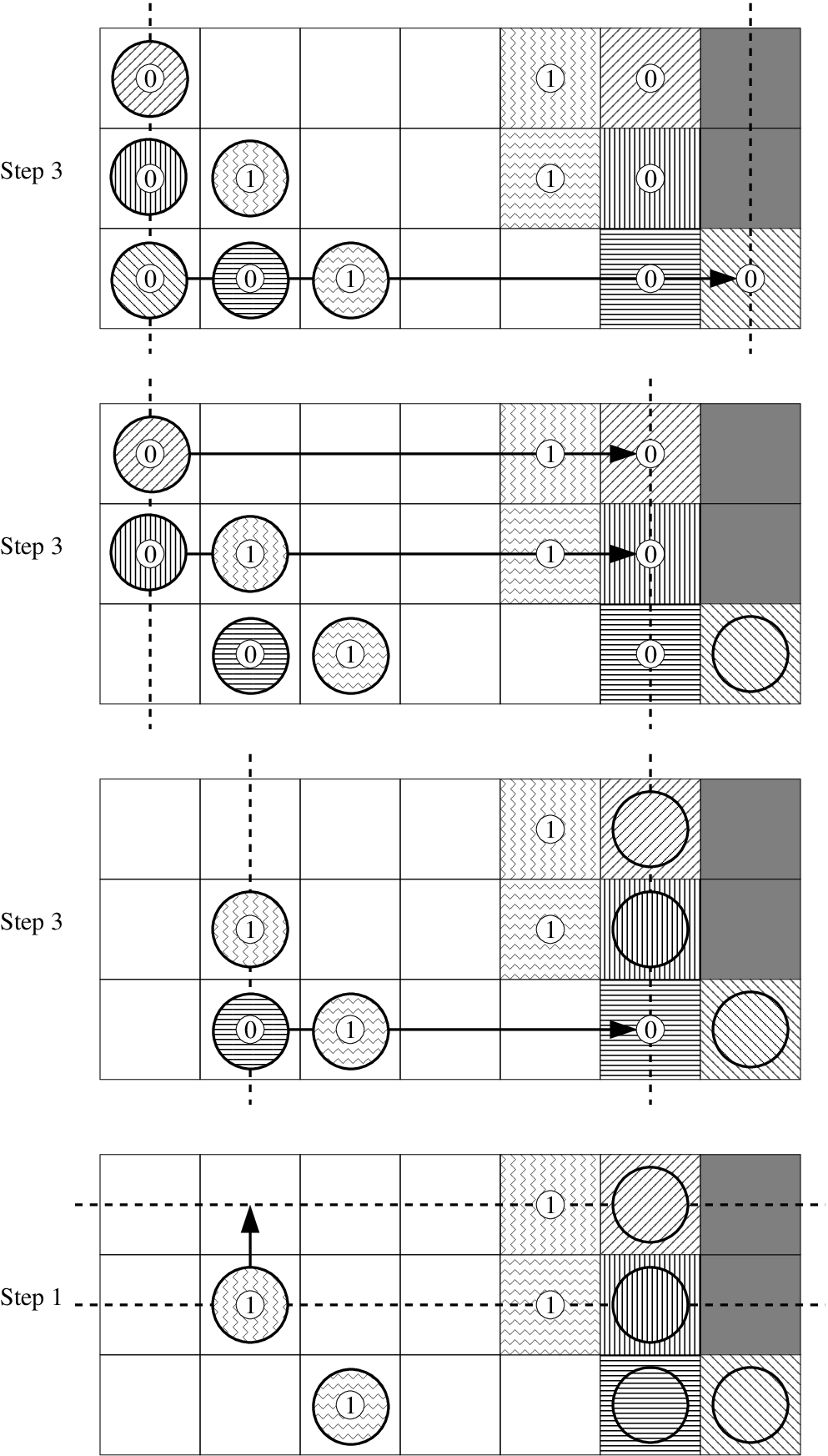
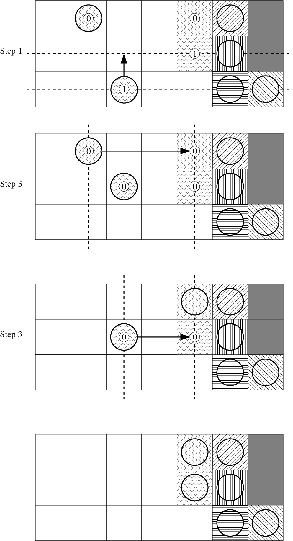
If any of the -tokens are ready, go to Step 2. Otherwise, perform a sequence of moves to shift all unplaced -tokens up one square. The reader can easily check that the sequence of moves accomplishes this. The assumption that is sufficiently large ensures that the upward movement of the -tokens is unobstructed. This step will decrease the readiness number of each -token by . Repeat this step until some -token is ready.
- 2.
Scan through the columns of , beginning with the rightmost column and proceeding to the left. Within each column locate the topmost square that does not already contain a -token. Let be the first ready square which we encounter in this way.
- 3.
Find a ready token in the same row as the square . Make the unique move which causes to move into . This may cause other tokens to move as well. All tokens which move here move to their final destination, so after this move, they and the squares they occupy are no longer considered ready.
- 4.
Repeat Steps 1 through 3 until every square of contains a -token.
Example 3.4.
Figures 3 and 4 illustrate the GRGA, applied to the example from Figure 2. We now draw only the squares in the upper right rectangle as these are the only ones relevant to the movement of the -tokens. Moreover, only the -tokens are shown in these diagrams, and the number on the token is the readiness number, not the token label. To specify the picture , each -token is given a shading and the corresponding square under in is shaded similarly. Each unshaded square actually contains a -token. The two darkly shaded squares in the upper right corner contain -tokens, as do each of the squares not shown in this diagram, but these squares are not part of the big region.
We now show that the GRGA accomplishes what it claims to accomplish.
Lemma 3.2.
Given a picture between and , the GRGA will win the game for .
Proof.
First note that after vertical movement from Step 1 is finished, the number of ready tokens in any row equals the number of ready squares in that row: an empty square is ready if and only if the -token which began in the square is in the same row as . We show that this equality is preserved, by showing that the move in Step 3 only ever causes ready tokens to move into ready squares.
Claim (i)
A move from Step 3 causes only ready tokens to move. In particular the number of ready tokens in a row always remains less than or equal to the number of ready squares in a row. The only tokens that can conceivably move are those in the same column as . Because is the top unfilled square in its column, no tokens above move. Because of Lemma 3.1 part (b), all tokens below are ready.
Claim (ii)
Only ready squares are filled. The algorithm attempts to fill the rightmost squares first. If there is a ready square in some column, the topmost empty square in that column will also be ready, by Lemma 3.1 part (d); thus the algorithm will never fill any square left of before it fills . However, by Lemma 3.1 part (c) the ready squares are rightmost in their row. Thus if a token moves into a non-ready square, it means that there are no ready squares in its row. But since only ready tokens move, we would have a row with at least one ready token and no ready squares. This, as noted in Claim (i), is impossible.
Claim (iii)
The move from Step 3 is always possible. Since only ready squares are filled by ready tokens, the number of ready squares and ready tokens in any given row is always equal. Thus there is a ready token in the same row as the ready square . Because we assume to be sufficiently large, is to the left of . If is in column and is in column , the move will take the token into square .
Thus in Steps 2 and 3, every ready square eventually gets filled by a ready token: by the argument in Claim (ii) no square is skipped. However, because the readiness numbers are initially non-negative and Step 1 decreases the readiness number of each square by , every square of is ready at some point; thus the algorithm puts a -token in each square of , at which point the game is won. ∎
Proof of Theorem 2.
() For we use the GRGA, which wins the game by Lemma 3.2. For , we proceed by induction. Suppose . Then we can write
| (5) |
in the Schubert basis, where , and
Since this is really a Grassmannian calculation, will be necessarily be of the form for some -string . By Lemma 3.2 we can win the game corresponding to , only moving -tokens. It is easy to see that exactly the same sequence of splittings and moves can be made in the game for , and that it causes the -tokens to end up in exactly the same final positions. Note that we end up with either a -token or an -token in every square which does not correspond to an inversion of , i.e. every square which does correspond to an inversion of .
This sequence of moves no longer wins the game; however, we can proceed inductively, after two further small steps. First, we perform a sequence of splittings so that every -token is in a one-square region of its own. Next, after splitting in this way, we replace each -token by an -token. This second step is not a legitimate play in the game, but it is completely harmless: because every -token is sequestered in its own one-square region, it can have no effect whatsoever on any possible subsequent moves of the game. But now we have precisely reached the initial position of the game corresponding to . This is again a game associated to a Grassmannian problem, and by Equation (5) the Schubert intersection number is non-zero. By induction, there is a sequence of moves to win this new game. Thus by concatenating the two sequences of moves, we can win the original game. ∎
4 Remarks
In Step 3 of the GRGA, there is a somewhat canonical choice for the token , namely the leftmost ready token in its row. If we use this choice of , one can verify that the algorithm actually transports the -token which is initially in square to the square . On the other hand, if there is a way of winning the root game, there is generally a plethora of ways, most of which do not arise by following the GRGA for any picture. Theorem 2 tells us that the existence of any one way to win implies the existence of a picture between , and . However, given a sequence of moves which wins the game, it is not at all obvious how to construct such a picture. This is even unclear in the the case where , and only -tokens are moved.
It is worth noting that the root game can be used to determine whether
even if the cohomological degree of the product is not . To do this, we modify the game by changing the winning condition to read “the game is won if there is at most one token in each square”, rather than “exactly one token in each square”. Once we do this, we have the following corollary of Theorem 2.
Corollary 4.1.
Take suitably large, and let be obtained from as before. Then if and only if the root game for can be won with the modified winning condition.
Proof.
There is a small catch: with this more general winning condition, our observation in Remark 1.1 becomes invalid. There is no longer an easy necessary and sufficient condition indicating when splitting is advantageous.
One of the unfortunate features of this presentation is the asymmetry in the way the permutations are defined. The root game itself is manifestly symmetrical in the permutations given. However, because and are produced in a different way from , the symmetry is broken for Grassmannians. Nevertheless, as Theorem 2 is valid for any , we can formulate a symmetrical game by taking to be arbitrary, and , so that . To see how this new formulation changes the initial position, contrast Figure 5 with Figure 2.

The only splitting which occurs in the proof of Theorem 2 is before the first move, and in the inductive step. The GRGA itself does not split between moves. As noted in Remark 1.1, it can never be harmful to split maximally between moves, and it turns out that if one modifies the GRGA to split maximally between moves, things proceed very much as before. However, in the next section, our proof of Theorem 3 will rely on the fact that the GRGA involves no splitting.
It would be nice if we could take in Theorem 2. Although we are not aware of any example which proves that this cannot be done, the algorithm simply falls apart if is too small. There are several problems which occur with trying to follow a similar approach. The most serious of these is that a token may be to the right of the square for which it is supposedly destined according to the chosen picture. Again, this highlights the fact that we do not know a straightforward two-way correspondence between pictures and ways of winning the root-game. Instead, in the next section we prove Theorem 3, a geometrical analogue of Theorem 2 which is valid for all . Theorem 3 suggests that it is not unreasonable to conjecture that Theorem 2 is true for all . We leave it as an open problem to determine whether or not this is in fact the case.
5 Geometric interpretation
In [P] we give a complete description of the geometry underlying the root game. The picture is quite different from those found in the geometric Littlewood-Richardson rules of Vakil [V] and more recently Coskun [C], both of which study degenerations of intersections of Schubert varieties inside a Grassmannian—we would be surprised if there were any straightforward relationship. Our methods are based on studying tangent spaces to Schubert varieties, and are more closely related to the approach used by Belkale in his geometric proof of the Horn conjecture [B]. Here, we will recall only the parts of the picture which are most relevant to our situation.
In this section we shall once again assume . Our notation changes slightly from Section 1 in that we will be working with instead of .
Let denote the standard basis of . Let denote the standard Borel subgroup of (upper triangular matrices), and let denote its opposite (lower triangular matrices). As before will be the standard maximal torus. For any complex vector space let be the disjoint union of all Grassmannians , .
Let be a region in the game, and let
describe the configuration of the tokens within this region. In the underlying geometry there is, assigned to the combinatorial pair , a corresponding geometric pair , where is a -module, and is a -fixed point on (or equivalently the are -invariant subspaces of ). As a -representation, is multiplicity-free, and the distinct -weights are
The (distinct) -weights of correspond to the positions of the -tokens inside :
Thus the pair carries all relevant information about the region and the arrangement of the tokens with .
The region is solved when there is exactly one token in each square. In terms of the pair this is occurs when
| (6) |
We’ll call any which satisfies condition (6) transverse.
Assuming we do not split the region , a move or a sequence of moves in the game takes the pair to a new pair , where is in the -orbit closure through . Thus if we solve a region starting from position , we have located a transverse -fixed point .
The importance of transverse points in is seen in the following proposition.
Proposition 5.1 ([P]).
Consider the position of the root game game for which arises after splitting but before the first move is made. The tokens are in their initial position, but there may be more than one region. To each region there is an associated pair . Then
if and only if for every region there exists a transverse point .
Note that the point in Proposition 5.1 is not necessarily -fixed. The big question, therefore, is how specialised can we make the point and still have Proposition 5.1 be true. There are three levels of specialisation that we could request of this transverse point .
- 1.
is any transverse point in .
- 2.
is a -fixed transverse point in .
- 3.
is a (-fixed) transverse point in , where comes from applying sequence of root game moves (but no splitting) to the position .
A priori, it is not clear that these three levels of specialisation are equivalent. However, for Grassmannian Schubert calculus with sufficiently large, Theorem 2 shows that they are all equivalent. The GRGA tells us exactly how to produce a sequence of moves which gives the point at Level 3, which is the most specialised. Note it is important here that splitting is never used in the GRGA—when a region is split, the one is tempted to define need not be in .
Unfortunately, when is small the GRGA can fail, and so we cannot claim that all three levels of specialisation are equivalent for all . Our goal in this section is to show that even if is too small for the GRGA to work, we can still get at Level 2; i.e. Proposition 5.1 is still true for Grassmannian Schubert calculus if we demand that be a -fixed point.
To make matters more concrete, we now explicitly describe the initial pair for the big region in the root game associated to . This is the only region that we need to concern ourselves with, since all other regions are already solved.
Let be the space of matrices, having standard basis , and let act on by conjugation. Let denote the -submodule of generated by the entries in the upper right rectangle. Let be the -submodule of generated by such that contains a -token. Then is the quotient -module
Note has a basis . The point is described as follows:
Note that , so we need not give it much further consideration.
Let be the subspace of whose -weights correspond to :
and let . Note that , so the point is transverse.
Example 5.1.
For the initial position shown in Figure 2,
Theorem 3.
For every ,
if and only if with and as above, .
Proof.
Assume
We know the result is true for sufficiently large, since the GRGA tells us how to get from the position to the position . We use this fact to deduce the result for other values of .
For any two choices of , say and , we get different spaces , , etc. We distinguish these notationally by using (resp. ) to denote the space corresponding to (resp. ), and likewise for any quantity depending on . Note that is independent of .
For any fixed and , let be the linear map given by
Let be the dense open subset of ,
Then induces a map
Observe that . The idea is essentially to show that is dense in , and that . This implies that if , then . Hence if the result is true for , then the result will be true for .
We will only prove this in the case where and is arbitrary, and in the case where is arbitrary and . This is enough to give the result for all .
The case where is the easier of the two. The map
allows us to view as a subgroup of , and is a -equivariant inclusion. Moreover . Thus takes into .
For the case where , we consider the -orbit not through , but through a lifted point . is defined in the same way as : . Let be defined analogously to , taking a dense subset of to . It suffices to show that takes a dense subset of to a subset of .
Let be the subgroup of of block diagonal matrices of type . Now also acts on , and is fixed by . Since is dense in , it follows that the orbit is dense in .
Thus in fact it suffices to show that takes a dense subset of to a subset of . But this is true, as
whenever both matrices are invertible.
∎
Although Theorem 3 is a geometric statement, our proof ultimately relies on the combinatorics of the Littlewood-Richardson rule. The key non-geometric fact we use is that if and only if there exists a picture between and . It would be an interesting project to find a purely geometric proof of this theorem. The hope would be that a geometric proof of Theorem 3 might allow us to see how to generalise some of the results in this paper beyond the Grassmannian.
Acknowledgements
The author is grateful to Allen Knutson and Stephanie van Willigenburg for providing feedback and corrections on this paper.
References
- [B] P. Belkale, Geometric proofs of Horn and saturation conjectures, J. Algebraic Geometry 15 (2006), no. 1, 133-173.
- [C] I. Coskun, A Littlewood-Richardson rule for two-step flag manifolds, preprint: http://www-math.mit.edu/˜coskun/.
- [F1] W. Fulton, Young tableaux with applications to representation theory and geometry, Cambridge U.P., New York, 1997.
- [F2] W. Fulton, Eigenvalues, invariant factors, highest weights, and Schubert calculus, Bull. Amer. Math. Soc. 37 (2000), 209–250.
- [FG] S. Fomin and C. Greene, A Littlewood-Richardson miscellany, European J. Combin. 14 (1993), no. 3. 191–212.
- [KTW] A. Knutson, T. Tao, and C. Woodward, The honeycomb model of tensor products II. Puzzles determine facets of the Littlewood-Richardson cone, J. Amer. Math. Soc. 17 (2004), no. 1, 19–48 (electronic).
- [LR] D.E. Littlewood and A.R. Richardson, Group characters and algebra, Philos. Trans. Roy. Soc. London. 233 (1934), 99–141.
- [P] K. Purbhoo, Vanishing and non-vanishing criteria in Schubert calculus, Int. Math. Res. Not. (2006), 24590, 1–38.
- [RW] J.B. Remmel and R. Whitney, Multiplying Schur functions, J. of Algorithms 5 (1984), 471–487.
- [V] R. Vakil, A geometric Littlewood-Richardson rule, to appear in Ann. Math, arXiv preprint: math.AG/0302294.
- [Z] A.V. Zelevinsky, A generalization of the Littlewood-Richardson rule and the Robinson-Schensted-Knuth correspondence, J. Algebra 69 (1981), no. 1, 82–94.