To appear in the
Handbook of Knot Theory
William W. Menasco and Morwen B. Thistlethwaite, Editors
- 1.
Colin Adams, Hyperbolic knots
- 2.
Joan S. Birman and Tara Brendle Braids and knots
- 3.
John Etnyre, Legendrian and transversal knots
- 4.
Cameron Gordon Dehn surgery
- 5.
Jim Hoste The enumeration and classification of knots and links
- 6.
Louis Kauffman Diagrammatic methods for invariants of knots and links
- 7.
Charles Livingston A survey of classical knot concordance
- 8.
Marty Scharlemann Thin position
- 9.
Lee Rudolph Knot theory of complex plane curves
- 10.
DeWit Sumners The topology of DNA
- 11.
Jeff Weeks Computation of hyperbolic structures in knot theory
Computation of Hyperbolic Structures
in Knot Theory
1 Introduction
Knot and link complements enjoy a geometry of crystalline beauty, rigid enough that simple cut-and-paste techniques meet geometrical as well as topological needs, yet surprisingly complex in their inexhaustible variety. The cut-and-paste approach makes computer exploration of their geometry easy: link complements become finite unions of tetrahedra, handled in a purely combinatorial way, with no need for the messy machinery of differential geometry.
The present article begins with the geometry of 2-dimensional link complements in Section 2 to provide an overview of all the main ideas. Section 3 explains an efficient algorithm for triangulating 3-dimensional link complements, Section 4 shows how to compute the hyperbolic structure, and finally Section 5 shows how the hyperbolic structure deforms to yield hyperbolic structures on closed manifolds obtained by Dehn filling.
Readers may consult other chapters in this volume for richer discussions of hyperbolic knots and links [1] and Dehn fillings [2]. Hyperbolic structures have found applications in knot tabulation [3] and more generally provide a fast and effective way to test hyperbolic knots and links for equivalence [4] and to compute their symmetry groups [5, 6] and other invariants [7]. The computer program SnapPea [8] implements these applications based on the foundation described in the present article. The SnapPea source code contains detailed explanations of all algorithms used.
Even though the exposition in the present article is original, most of the mathematics was born in the work of Bill Thurston. Thurston’s informal 1979 notes (see also [9, 10]) contained the theory of hyperbolic knots and links, hyperbolic Dehn filling, and in particular his simple and elegant system (explained here in Sections 4 and 5) for finding hyperbolic structures in terms of complex edge angles.
2 Two-dimensional preview
Before tackling 3-dimensional knots and links, let us review the the 2-dimensional ones. Their topology and geometry is far simpler, yet the insights they provide will serve us well in the 3-dimensional case.


Just as a 3-dimensional link is a collection of 1-spheres (circles) in a 3-sphere, a 2-dimensional link is a collection of 0-spheres (pairs of points) in a 2-sphere. The classification of 2-dimensional links is easy: two links are equivalent if and only if they have the same number of components (Figure 1).
Each link complement admits a constant curvature geometry. The 0-component link complement, which is simply an unpunctured 2-sphere, already has spherical geometry. At first glance the remaining -component link complements, which are punctured 2-spheres, also seem to have spherical geometry, but these geometric structures are disallowed because they are incomplete. Many formal definitions of completeness appear in the literature, but intuitively a surface is incomplete if a traveller starting at some point on the surface can reach an “edge” (either a ragged edge or a boundary) within a finite distance. Conversely a surface is complete if a traveller starting at any point on the surface can travel any finite distance in any direction without hitting an edge. In the case of a punctured 2-sphere, a traveller easily reaches a puncture, so the surface is incomplete.
To construct a complete geometric structure on the 1-component link complement, pull the link itself (the pair of points) to infinity, dragging the link complement along with it (Figure 2, second frame). The link complement becomes an infinite cylinder, which has locally Euclidean geometry (constant zero curvature) and is complete.
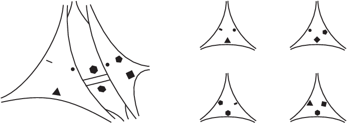
Following the same technique, take the 2-component link and pull the link itself (two pairs of points) to infinity. Intuitively the stretched out link complement looks hyperbolic (Figure 2, third frame). To make this rigorous, cut the link complement into four ideal triangles (Figure 3, left) and then define the hyperbolic structure on the link complement to be the union of four hyperbolic ideal triangles with edges identified (“glued”) in the appropriate way (Figure 3, right).
More generally, for every the -component link complement splits into a union of ideal triangles which then defines a hyperbolic structure on the link complement. The hyperbolic structure is never unique, but a simple Euler number argument shows that the number of ideal triangles must be exactly . An ideal triangle has area , so the total area of the -component link complement is no matter what hyperbolic structure is chosen.
Assuming we identify the ideal triangles’ edges
midpoint-to-midpoint (the midpoint of an edge being the edge’s
intersection with an orthogonal line of mirror symmetry), the
hyperbolic structure is complete, and is therefore called a complete hyperbolic structure. The parts stretching off to
infinity are called cusps.

On the one hand, ideal triangles are rigid
(Figure 4 left). On the other hand, the
gluing between two ideal triangles is flexible: each edge is
infinitely long so the neighboring triangles may slide past one
another (Figure 4 right). These
2-dimensional facts are exactly the opposite of the situation in 3
dimensions, where ideal tetrahedra are flexible but the gluings
between them are rigid. Nevertheless, deforming the hyperbolic
structure produces analogous results in both 2 and 3 dimensions,
and so examining the 2-dimensional case in this Section will
provide insight into the analogous 3-dimensional results in
Section 5.


To deform a hyperbolic structure, start with one of the cusps. Slice the cusp open (Figure 5). Gluing opposite edges of the sliced-open cusp straight across (Figure 5 top) would restore the cusp to its original condition, but gluing opposite edges with a shift (Figure 5 bottom) yields a different result. If you physically construct a paper model11 1 The paper model is of course only an approximation. The real cusp is intrinsically hyperbolic while your paper model is intrinsically flat. Nevertheless the paper model suffices for the demonstration at hand. Remember that the width of your paper strip must shrink exponentially fast as you move along it lengthwise. of the sliced-open cusp and wrap it around so that each point on one edge glues to a point on the opposite edge that’s shifted by, say, 4 cm, you obtain a cylinder (Figure 6). Your paper strip, if infinitely long, would wrap around the cylinder infinitely many times, approaching but never reaching a limiting circle.

Globally, for each 0-sphere in an -component link, pick a geodesic edge connecting the two cusps belonging to that 0-sphere. Cut, shift and reglue along each such edge (Figure 7 left). Locally the result at each cusp looks like Figure 6. Globally the result looks like Figure 7 right. That is, the result is a surface of genus with circles missing (namely the limiting circles of the former cusps). With foresight we may arrange for the geodesic edges (along which we cut, shifted and reglued) to be edges of the triangulation. That is, our original cusped surface was the union of hyperbolic ideal triangles, and we cut, shifted and reglued along edges of that ideal triangulation. Thus the result (Figure 7 right) is also the union of hyperbolic ideal triangles and therefore enjoys a hyperbolic structure, albeit an incomplete one. The missing circles are geodesics. Adding those missing geodesic circles yields a complete hyperbolic structure on the closed surface of genus .
In two dimensions most link complements admit a complete hyperbolic structure. Deforming a complete hyperbolic structure yields a hyperbolic structure (with missing geodesics) for a closed surface. Both these results generalize readily to three dimensions.
3 Triangulation of knot and link complements
Just as every 2-dimensional link complement splits into ideal triangles (Figure 3), every 3-dimensional link complement splits into ideal tetrahedra. For now we will work with “topological ideal tetrahedra” — that is, we will visualize them as ideal tetrahedra but won’t worry about the exact hyperbolic geometry they carry. The latter will be the subject of Section 4.
The goal in triangulating a link complement is to produce a triangulation that quickly simplifies down to as few tetrahedra as possible. Minimizing the number of tetrahedra saves space and computational time, but more importantly it vastly improves the chances that all tetrahedra will be “positively oriented”, a condition needed to rigorously guarantee that the subsequent hyperbolic structure is correct. The triangulation algorithm used in the computer program SnapPea has proven more effective than several alternatives the author tested, so that is the algorithm presented here.
Technical Note (which the reader may ignore): SnapPea’s algorithm
requires a connected link projection. If a given link projection
consists of more than one component, SnapPea does Type II
Reidemeister moves to make the projection connected. In the same
spirit, to each obviously unknotted component SnapPea does a
Type I Reidemeister move to add a nugatory crossing. Link
projections requiring these moves never have hyperbolic
complements; the moves are needed only for non-hyperbolic knots
and links.
The link complement will have one cusp for each component of the link. For visual convenience we chop off the cusps. That is, rather than triangulating the complement of the link using ideal tetrahedra, we’ll triangulate the complement of a tubular neighborhood of the link using truncated ideal tetrahedra. Once such a truncated ideal triangulation is found, the extension to true ideal tetrahedra is easy and obvious.
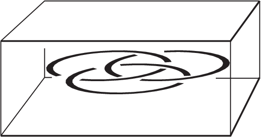
Imagine the tubular neighborhood of the link lying near the equatorial 2-sphere of the 3-sphere . To keep the construction simple and natural, the triangulation must adhere closely to the link projection itself. To accomplish this, let us triangulate it in rather than in (Figure 8). The two missing solid balls — one lying to either side of in — will be added back later.
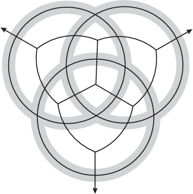
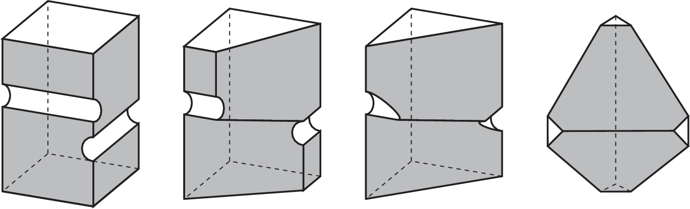
To triangulate the link complement in , cut straight down through it just as you would cut cookie dough with a cookie cutter. Figure 9 shows the pattern of the cuts: cut along the centerline of each link component and also along the dual graph. The resulting pieces are all identical. Figure 10 (first panel) shows one piece. It’s not yet a truncated tetrahedron. It has four truncated vertices, two of which border the tubular neighborhood of the knot and two of which border the upper and lower surfaces of , along with six ordinary faces, four of which are combinatorial hexagons and two of which are combinatorial squares.
Now deform each combinatorial square to become a tall narrow rectangle (Figure 10 second panel) that finally collapses to a vertical line segment (third panel). The resulting solid (last panel) has four truncated vertices (all are triangles) and four ordinary faces (all are hexagons), and is in fact combinatorially a truncated tetrahedron!
Collapsing all square faces to vertical lines does not change the
topology of the manifold. If some link component had only
overcrossings or only undercrossings, then collapsing the squares
would indeed change the manifold’s topology because we’d be
collapsing an embedded cylinder, but the preceding Technical Note
excludes this possibility. Collapsing an embedded square or a
series of embedded squares is safe.
A simple indexing system describes the triangulation in a format amenable to computer use. Label the four truncated vertices of each tetrahedron with the integers and label each face with the index of its opposite vertex. To specify how a face of one tetrahedron glues to a face of another, simply specify the permutation of the vertex index set induced by reflecting the vertices of the original tetrahedron across the face in question onto the vertices of the neighboring tetrahedron.
In general the vertex indices may be assigned arbitrarily, but in
the case of a triangulated link complement we make the convention
that vertex 0 is the truncated vertex at the south pole of
(on the bottom of the polyhedron in
Figure 10 left), vertex 1 is the
truncated vertex at the north pole of (on the top of the
polyhedron in Figure 10 left), and
vertices 2 and 3 are the truncated vertices touching the link (
the left and right hemi-cylindrical truncated vertices,
respectively, in Figure 10 left).
With this convention the symmetry of the decomposition guarantees
that all gluing permutations are the same throughout the
triangulation, namely .

We now have a nicely triangulated manifold, but we constructed it in rather than , so in it’s the complement of the link plus two solid balls. To remedy this problem, drill out a tube connecting the thickened link to the solid ball at the north pole (thus “cancelling” that solid ball) and a second tube connecting the thickened link to the solid ball at the south pole. The easiest way to drill out a tube is to splice into the triangulation a triangular pillow that already contains a pre-drilled tube (Figure 11). That is, let be any 2-cell of the triangulation incident to both the northern spherical boundary of and one of the torus boundary components of the link complement. If we cut along , insert an ordinary (un-drilled) triangular pillow, and reglue, then the topology of the manifold does not change. But if we instead insert a triangular pillow with a pre-drilled tube (Figure 11) then the boundary component at one end of the tube gets joined to the boundary component at the other end of the tube. In the present case this joins the spherical boundary component at the north pole (resp. south pole) to the torus boundary of the link, thereby neutralizing the former.
A triangular pillow with a pre-drilled tube can be constructed from two truncated (or ideal) tetrahedra. Face 0 of the first tetrahedron glues to face 0 of the second tetrahedron via the gluing . Face 3 of the first tetrahedron glues to face 3 of the second tetrahedron via the gluing . Faces 1 and 2 of the second tetrahedron glue to each other via the gluing . Faces 1 and 2 of the first tetrahedron remain unglued and provide the two external boundary faces of the pillow.
Once the two triangular pillows are installed we have a valid triangulation of the link complement. The triangulation contains tetrahedra, but the number of tetrahedra decreases substantially when the triangulation is simplified. Two elementary operations serve to simplify the triangulation: the first operation replaces three tetrahedra surrounding a common edge with two tetrahedra sharing a common face, while the second operation cancels two ”flattened” tetrahedra that share two adjacent faces. For an explanation of an effective high-level algorithm governing the application of the two elementary operations, please see the file simplify_triangulation.c in the SnapPea source code [8]. Note that the high-level algorithm sometimes requires the inverse of the first operation, which temporarily increases the number of tetrahedra – by replacing two tetrahedra sharing a face with three tetrahedra surrounding an edge – but ultimately leads to simplifications.
4 The complete hyperbolic structure
If the link complement admits a hyperbolic structure [1], then the “topological ideal tetrahedra” of the previous section may be replaced with honest hyperbolic ideal tetrahedra.
In principle this is easy: just imagine the topological ideal triangulation sitting in the hyperbolic manifold in some wiggly way, and pull all its 1-dimensional edges taut, so that the edges become geodesics running from infinity in one cusp, though the fat part of the manifold, and back to infinity either in the same cusp or in a different cusp. Each 2-dimensional face is now defined by its three geodesic edges, and each 3-dimensional ideal tetrahedron is defined by its faces.22 2 If the triangulation is inefficient, with more than a minimal number of tetrahedra, then there is some danger that one or more of the tetrahedra will become negatively oriented — in effect the triangulation folds over on itself and then double back at those places, leaving some points in the manifold covered three times, twice by ordinary positively oriented tetrahedra and once by a negatively oriented tetrahedron. But we needn’t worry about this problem here.


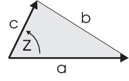

In practice we solve for the shapes of the honest hyperbolic ideal tetrahedra analytically. The shape of an ideal tetrahedron is determined by its dihedral angles. By symmetry (Figure 12) opposite dihedral angles are equal, so three of the angles determine the opposite three. Furthermore, if we examine a horospherical cross section of a cusp (Figure 13), we may replace the real dihedral angle with a complex dihedral angle (Figure 14). The three complex dihedral angles depend on each other: any one of them determines the other two (Figure 15). Thus a single complex dihedral angle completely parameterizes the shape of an ideal tetrahedron.

The real dihedral angles surrounding a single edge in a hyperbolic ideal triangulation sum to . Analogously, the complex dihedral angles surrounding an edge multiply to . Figure 16 illustrates how the complex angles provide more information than the real angles do. In practice one replaces the product with its more powerful logarithmic form to insure that the arguments sum to rather than, say, to or . Geometrically this ensures that the sequence of tetrahedra wraps exactly once around the edge.

Our goal, in geometrical terms, is to take the topological ideal triangulation of a knot or link complement produced in Section 3 and realize each topological ideal tetrahedron as an honest hyperbolic ideal tetrahedron in such as way that they fit together correctly around their common edges. Algebraically, this means we must find complex dihedral angles for the tetrahedra such that the edge equations are satisfied. But we are not quite ready to solve those equations. Even though a simple Euler characteristic argument guarantees that the number of equations equals the number of variables, the equations are not independent. Rather the solution space contains one complex degree of freedom for each cusp (i.e. for each component of the original link). For now we will resolve this ambiguity by insisting that each cusp be complete, i.e. that its cross section be effectively a parallelogram (Figure 17 left) rather than some other quadrilateral (Figure 17 right). Section 5 will explore the more general case in detail.
In summary, to the set of edge equations we add a set of cusp equations ensuring that each cusp is complete. We then solve the equations using Newton’s method and obtain the solution.
In practice the situation is somewhat delicate. When applied
blindly, Newton’s method usually fails. That is, if one begins
with, say, regular ideal tetrahedra (all complex dihedral angles
equal to the sixth root of unity ) and applies the standard Newton’s method, often the
shapes of the tetrahedra will diverge to infinity or other
nonsense values. To avoid this, one must take two precautions.
First, one re-selects the coordinate system at each iteration of
Newton’s method in order to minimize exposure to singularities and
keep the entries in the derivative matrix small. Second, one
trusts the direction of the gradient in Newton’s method but
distrusts its magnitude. Let us consider each of these two
precautions in detail.
Choice of coordinates. Complex dihedral angles of = 0, 1, or correspond to degenerate tetrahedra. Near those values, bad things happen. The two main problems are that (1) some of the entries in the derivative matrix (used in Newton’s method) approach infinity, and (2) incrementing the solution can move it too close to a singularity, resulting in wild swings in the real dihedral angles. Switching the coordinates from the complex dihedral angle to its logarithm helps a bit. Rather than having two singularities (at and ) embedded in the parameter space, you have only one. The singularity that used to be at is now at , but the singularity that used to be at has been happily pushed out to infinity.
This strategy can be further improved by choosing the (logarithmic) coordinate system based on the current shape of the tetrahedron. The coordinate system is chosen so that the current shape of the tetrahedron stays as far away as possible from the one remaining singularity in the parameter space. Specifically, let the three complex dihedral angles be
| (1) |
(note that those expressions are taken directly from the formulas in the caption of Figure 15) and divide the complex plane into three regions
| Region A: | and | ||
|---|---|---|---|
| Region B: | and | ||
| Region C: | and |
Viewed on the Riemann sphere, the singularities at , and are equally spaced points on the equator, and the Regions A, B and C are separated by meridians spaced apart. Points lying on the separating meridians may be arbitrarily assigned to either neighboring region.
When lies in Region A (resp. Region B, Region C), let (resp. , ) parameterize the shape of the
tetrahedron.
Proposition. If one chooses coordinates as
in the preceding sentence, then the entries in the derivative
matrix remain bounded.
Proof. Each entry in the derivative matrix used in Newton’s method is a fixed linear combination of the derivatives of , and for several tetrahedra, so it suffices to show that each such derivative has modulus less than or equal to one. First compute
| (2) |
and then take ratios of the above to obtain
| (3) |
If lies in Region A and we have chosen coordinates as required, then the derivatives in the first column of (3) have modulus less than or equal to 1. This is obvious for the first entry in the column. For the third entry it’s an immediate consequence of the condition . For the second entry, note that
and
so .
Similar arguments show that when lies in Region B (resp.
Region C) the derivatives in the second column (resp. third
column) have modulus less than or equal to 1. Q.E.D.
Theoretical Note #1: The computed dihedral
angles, given by the imaginary parts of , and
, are not a priori limited to the range .
However, only when they fall in the range does the
computed solution have a direct geometrical interpretation as a
union of ideal tetrahedra comprising a cusped hyperbolic
3-manifold. When some or all of the angles fall outside the range
the situation is more complicated: in most cases the
hyperbolic structure still exists and has the computed volume but
in rare cases spurious non-geometric solutions occur.
Theoretical Note #2: I briefly entertained the
idea of finding a single coordinate system that avoids all three
singularities. Unfortunately Picard’s Little Theorem shows that
this is not possible for an analytic function. It might be
possible for a nonanalytic function — perhaps a simple function
of and — but I haven’t pursued this idea and in any
case such a function wouldn’t be conformal.

Avoiding singularities. When applying Newton’s method to find a hyperbolic structure, one trusts the direction of the gradient but distrusts its magnitude. More precisely, one insists that neither the real part nor the imaginary part of the parameter change by more than for any tetrahedron. This restricts the change to a limited zone (Figure 18) and in particular keeps the parameter well away from the one singularity that remains in the parameter space (at or ). If Newton’s method calls for a change exceeding those limits, then we rescale the proposed change (for all the tetrahedra, not just the offending one) so that the largest change in any or is .
5 Hyperbolic Dehn filling
Section 2 showed how to construct a hyperbolic structure on the complement of a -component link of 0-spheres on a 2-sphere () and then went on to show how deforming the hyperbolic structure (Figures 5 and 6) yields a hyperbolic structure on a closed surface of genus with two closed geodesics missing (Figure 7). That was 2-dimensional hyperbolic Dehn filling. Three-dimensional hyperbolic Dehn filling is similar: deforming the complete hyperbolic structure on a -component link complement (Section 4) will yield a hyperbolic structure on a closed manifold with closed geodesics missing. In spite of the strong analogy between 2-dimensional and 3-dimensional hyperbolic Dehn filling, there are nevertheless a few differences. In the 2-dimensional case the ideal triangles were rigid while the gluings between them were flexible, whereas in the 3-dimensional case the shapes of the tetrahedra themselves are flexible while the gluings between them are rigid. More interestingly, in the 2-dimensional case different deformations all gave the same topological 2-manifold (namely the closed surface of genus , once the missing geodesics are filled in), whereas in the 3-dimensional case different deformations give topologically distinct 3-manifolds (filling in the missing geodesics realizes a Dehn filling on the link complement, with the Dehn filling coefficients depending on the deformation — more on this below).

The cut-open 2-dimensional cusps of Figure 5 become, in three dimensions, solid structures resembling the Eiffel tower (Figure 19). If the cusp cross section is effectively a parallelogram (Figure 17 left) the sides of the Eiffel tower match straight across (Figure 19 left) in the sense that people travelling across one face of the tower will re-enter the opposite face on the same level at which they left. This condition ensures that the hyperbolic structure is complete. If, on the other hand, the cusp cross section is not a parallelogram (Figure 17 right), then the sides of the Eiffel tower match with a vertical offset (Figure 19 right). For example, travellers leaving the tower at point on one level will re-enter at point on a lower level. Note that the width of the upper quadrilateral’s long side equals the width of the lower quadrilateral’s short side.

Henceforth we will restrict our attention to the case that the offset in one direction is a rational multiple of the offset in the transverse direction (Figure 20). Cutting along a consistent set of cross sections (like those illustrated in Figure 20) splits the cusp into an infinite set of bricks, all of equal height. Ignore for a moment the bricks’ freshly cut top and bottom faces, and instead glue them together along their side faces. The result will be a solid cylinder (Figure 21) with infinitely many progressively narrower bricks spiraling in towards the center. The vertical geodesic at the exact center is missing, and indeed plays the role in three dimensions of the missing geodesics in Figure 7. Restoring the gluings on the bricks’ top and bottom faces converts the cylinder into a solid torus, still with its central geodesic missing. Typically the cylinder’s bottom glues to its top with some nonzero twist.


Filling in the missing geodesic at the center of the solid torus (Figure 21) realizes a Dehn filling on the link complement. To read off the Dehn filling coefficients, simply note how a meridian of the solid torus wraps around the cusp. In the example shown (see Figure 22 for a top view) any topological meridian will wrap times around the quadrilateral’s “long direction” and times around its “short direction”. Typically the “long direction” is chosen to be a longitude of the original knot or link while the “short direction” is chosen to be a meridian of the original link, making this a Dehn surgery.
In practice, of course, we don’t randomly deform the hyperbolic structure and then wait to see what Dehn filling coefficients emerge. Instead, we choose the Dehn filling coefficients in advance and ask what deformation of the hyperbolic structure will accommodate them. Recall from Figure 17 that a product of complex dihedral angles gives the rotational/dilational factor taking one side of the quadrilateral to the other. In Section 4 we insisted that that product be ; more precisely we replaced the naive product equation with the more powerful logarithmic equation to guard against stray multiples of . Here we apply the same technique, but focusing on the arbitrary quadrilateral (Figure 17 right) instead of the parallelogram (Figure 17 left). We now get one expression for the rotation/dilation in the meridional (“short”) direction and a different expression for the rotation/dilation in the longitudinal (“long”) direction. Tracing all the way around the loop in Figure 22 returns us to our starting point with a rotation. The loop consists of meridians and longitudes, so the analytic condition is
| (4) |
In Section 4 we had supplemented the
edge equations with the cusp equations to solve for the hyperbolic
structure on the cusped manifold. We now instead supplement the
edge equations with the Dehn filling equations (4)
to solve for the hyperbolic structure on the Dehn filled manifold.
Acknowledgement. I thank Adam Weeks Marano for help with the illustrations.
References
- [1] C. Adams, “Hyperbolic knots”, this volume.
- [2] C. Gordon, “Dehn surgery”, this volume.
- [3] J. Hoste, “The enumeration and classification of knots and links”, this volume.
- [4] J. Weeks, “Convex hulls and isometries of cusped hyperbolic 3-manifolds”, Topology Appl. 52 (1993) 127–149.
- [5] S. Henry and J. Weeks, “Symmetry groups of hyperbolic knots and links”, J. Knot Theory and Its Ramifications 1 (1992) 185–201.
- [6] C. Hodgson and J. Weeks, “Symmetries, isometries and length spectra of closed hyperbolic 3-manifolds”, Exp. Math. 3 (1994) 261–274.
- [7] C. Adams, M. Hildebrand and J. Weeks, “Hyperbolic invariants of knots and links”, Trans. Amer. Math. Soc. 326 (1991) 1–56.
- [8] J. Weeks, “SnapPea: a computer program for creating and studying hyperbolic 3-manifolds”, available for free download from www.geometrygames.org.
- [9] W.P. Thurston, “Three dimensional manifolds, Kleinian groups and hyperbolic geometry”, Bull. (New Series) Amer. Math. Soc. 6 (1982) 357–381.
- [10] W.P. Thurston, Three-dimensional geometry and topology (1997) Princeton Mathematical series 35, Ed. S. Levy, (Princeton University Press, Princeton, USA).