Table of Contents for the Handbook of Knot Theory
William W. Menasco and Morwen B. Thistlethwaite, Editors
- (1)
Colin Adams, Hyperbolic knots
- (2)
Joan S. Birman and Tara Brendle Braids and knots: A survey
- (3)
John Etnyre, Legendrian and transversal knots
- (4)
Greg Friedman Knot spinning
- (5)
Jim Hoste The enumeration and classification of knots and links
- (6)
Louis Kauffman Knot Diagrammatics
- (7)
Charles Livingston A survey of classical knot concordance
- (8)
Lee Rudolph Knot theory of complex plane curves
- (9)
Martin Scharlemann Thin position in the theory of classical knots
- (10)
Jeff Weeks Computation of hyperbolic structures in knot theory
Thin position in the theory of classical knotsThanks: Research supported in part by an NSF grant.
For our purposes, “knot theory” will have the narrowest interpretation: the study of isotopy classes of locally flat embeddings of the circle in . The distinctions between smooth, PL, and locally flat topological embeddings are usually unimportant in these dimensions so, for convenience, we’ll use language that is typically associated with the smooth category. For example, a knot is a smooth submanifold of diffeomorphic to . The focus of this article will be on a particular technique for analyzing knots, called “thin position”. Much like the study of crossing diagrams, it’s a technique that exploits very heavily the fact that the ambient manifold is and not another manifold, not even a possibly alternate homotopy sphere. The roots of the technique might be traced back to Alexander’s proof [Al] of the Schönfliess theorem, in which he imagines a horizontal plane sweeping across a sphere embedded in -space and examines the intersection set during the sweep-out. The modern use began with a stunning application by David Gabai, in his proof that knots in satisfy Property R [Ga].
This is mostly an expository survey; one bit of new mathematics is an updated application of thin position to the proof that Heegaard splittings of are standard (cf. Corollary 5.13).
1. From crossing number to bridge number
One way, perhaps historically the first way, of thinking about knots in is this: Choose a point in . A knot in is generically disjoint from , as is an isotopy between knots. Thus knot theory in (narrowly defined, as above) is equivalent to knot theory in . Once we think of a knot as lying in , it’s natural to imagine projecting it to ; this is what we do when we draw the knot. A generic such projection will look like an immersed closed curve in the plane having only double points. If we keep track, at the double points, of which strand in the original knot passes over the other we have the classical description of a knot via its crossing diagram. Crossing diagrams are one of the oldest and most naive ways of trying to classify knots, but their importance has been re-emphasized by the modern discovery of new knot invariants, invariants that are most easily described via these projections. Unlike more sophisticated invariants (coming, for example, from the algebraic topology of the knot complement) it is clear that knot projections make immediate use of the fact that the ambient space is the -sphere, and not some other manifold.
The first knot invariant that is suggested by knot projection is the crossing number of the knot. For a generic projection of the knot to the plane, the crossing number of the projection is just the number of double-points of the projection. An isotopy of the knot may reduce this number; the crossing number of the knot is defined as the minimum number that can be achieved via an isotopy of the knot in -space. The crossing number is the most natural invariant for cataloguing knots via their projections (it is the basis of the standard knot tables) but otherwise it is not a particularly good invariant. For a given knot, while it’s easy to find an upper bound for the crossing number (just use any projection), there isn’t a natural way to find the projection that minimizes the crossing number. In particular, the behavior of the invariant under e.g. knot sum is not well-understood.
There is another invariant, much like the crossing number and only slightly more difficult to describe, that is in fact remarkably well behaved under knot sum. Suppose one starts with a knot projection, and a point on the knot, and starts moving along the knot, recording at each crossing whether one is on the upper strand (an overcrossing, say marked with a ) or on the lower strand (an undercrossing, say marked with a ). Continue in this way around the entire knot and examine the result. It is a sequence of signs, e. g. . The number of signs recorded is twice the number of crossings of the projection since in a trip around the knot, one passes through each crossing twice. For the same reason there will be as many as signs. Now, instead of considering the number of crossings of the knot (i. e. focusing on the number of and signs) consider the number of times that the sign recorded changes. If the last sign differs from the first, record that also as a change, as if one were viewing the pattern of and on a circle. Thus for the sequence the number of changes is . Of course the number of changes is necessarily even. Half that number (i.e. the number of strings of consecutive ’s, say) is called the bridge number of the knot projection. Just as with the crossing number, the bridge number of the projection may change as the knot is isotoped; the minimum that can be achieved by an isotopy of the knot is called the bridge number of the knot. For reasons that will be apparent, the bridge number of the unknot, which has no crossings, is conventionally set to be . This invariant was introduced by Schubert [Schub].
The terminology “bridge number” is meant to evoke the following picture: if a knot projection has bridge number , that means there are sign changes from to or vice versa; equivalently, each sign lies in one of strings of consecutive signs. Each string of consecutive signs corresponds to a strand of the knot which can be thought of as lying just above the plane. Between these strands are strands with only crossings; these can be thought of as lying on the plane. Thus the bridge number of the knot is the minimum number of bridges that one would need to erect on the plane so that the entire knot could be put on the plane and on the bridges, with crossing over each bridge exactly once. Schubert [Schub] proved that this invariant is essentially additive. To be precise, is additive; that is,
or
A modern proof is given in [Schul].
Schubert’s remarkable result suggests that there should be a more natural way of viewing bridge number. Consider the description of the knot just given: lying mostly on the plane, but with certain sections of it elevated above the plane on bridges. The original perspective on the knot is the bird’s-eye view in which we look down on the knot from above. Imagine instead the perspective of someone standing on the plane, looking sideways at the knot and thinking about the height of the knot above the plane. That is, instead of the projection that described the original knot projection, consider instead the projection defined by height above the plane. Then will achieve a single maximum on each bridge, and each pair of successive maxima is separated by a minimum corresponding to a strand of that lies on the plane. In other words, if is put on bridges, then has maxima. This number of maxima can be preserved even when is moved slightly to make it generic with respect to the height function by, for example, putting a bit of a dip into the level strands lying on the plane. In other words, we have the following:
Proposition 1.1.
Suppose has a projection with bridge number . Then may be isotoped so that the standard height function restricts to a Morse function on with maxima and minima.
Conversely, we have
Proposition 1.2.
Suppose , and the standard height function restricts to a Morse function on with maxima and minima. Then .
Proof.
Each point on at which has a local maximum can be pushed even higher by an isotopy of , say along a path that rises from the maximum and, by general position, misses the rest of as it rises. Similarly, each point at which has a local minimum can be pushed lower. So with no loss, may be isotoped so that all the maxima occur near the same height (say ) and similarly all the minima occur near the same height (say ). Consider how the plane divides : cuts into strands, above the plane, each containing a single maximum, and below the plane, each having a single minimum.
The plane slightly above height cuts off tiny strands of , one for each minimum, that lie below the plane. These are clearly isotopic rel their endpoints to disjoint arcs in . See Figure 1. Between the heights and there are no critical points of on . It follows that in fact all strands of lying below can be simultaneously isotoped rel their ends to lie on . Similarly, all strands of lying above can be isotoped rel their end points so that they consist of level arcs in a plane just above , together with vertical arcs at their end points between and . When viewed from above as projected onto , then has a projection with bridge number no higher than . ∎

Combining the two propositions above gives a more natural definition of bridge number of a knot : take the number of maxima that the standard height function has on the knot (in general position with respect to ) and minimize that number via an isotopy of . The result is the bridge number of . If there is a horizontal plane with the property that all maxima of lie above and all minima lie below it, then is said to be in bridge position with respect to ; the plane is called a dividing plane for . Any knot can be isotoped so that it is in bridge position, with maxima and minima.
2. From bridge number to width
Consider the critical values of in general position with respect to , the standard height function. As noted above, it’s always possible to isotope so as to raise the height of a maximum or to lower the height of a minimum, without affecting the height of any other critical point. Indeed there is such an isotopy whose support on is limited to a neighborhood of the critical point whose height is changed. Similarly, there is no difficulty lowering the height of a maximum through an interval that contains no other critical values, since by standard Morse theory, the preimage of an interval without critical values is a simple product. Combining these two observations, it’s easy to isotope to interchange the heights of critical points whose critical values are adjacent, so long as both critical points are maxima, or both are minima.
The only difficulty in rearranging the heights of critical points is the interchange of two adjacent critical values in which the higher value is a maximum and the lower value is a minimum. Informally, this can be described as moving a maximum down past a minimum. Such a move may or may not be possible, depending on the structure of the knot (cf Figure 2). It’s reasonable then to think of this move (pushing a maximum down past a minimum) as simplifying the picture of the knot, when it can be done; the point of thin position is to formally capture this idea in a useful way.

Let be a knot in general position with respect to the standard height function . That is, is a Morse function for which no two critical points have the same critical value. For each let denote the plane . If is a regular value for then crosses transversally, necessarily in an even number of points. The number changes only at critical values, where it increases by two at each minimum and decreases by two at each maximum. So if are the critical values of and values are chosen so that , then the function is determined by the sequence . That sequence is unchanged by pushing a maximum down past another maximum (or a minimum past another minimum) but is affected by pushing a maximum down past a minimum. In the last case, if the critical values are , then the reordering changes to and has no other effect. See Figure 3. More dramatically, if can be isotoped so that the maximum and its adjacent minimum cancel, then both and disappear and so both disappear from the sequence.
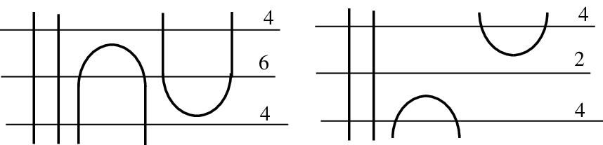
These changes are so straightforward, they suggest the following definition:
Definition 2.1.
Suppose, as above, is in general position with respect to the standard height function , are the critical values of and regular values are chosen so that . The width of K with respect to , denoted by , is . The width of K, denoted by , is the minimum of over all knots isotopic to . We say that is in thin position if
There is a small technical advantage in modifying this definition slightly so that it can be applied directly and a bit more usefully in the compact situation . Define the standard height function as the composition of the inclusion and the standard projection onto the last factor of . Then has two critical points on (called the north and south poles). A knot in general position with respect to will be disjoint from these poles, and the above definition can be restated for this height function. The most significant difference with this definition is that (for ), is now a -sphere instead of a plane; if is in bridge position, then what divides the maxima from the minima is a dividing sphere instead of a dividing plane. Whenever is a regular value for , we continue to denote by .
Note that if or has been isotoped to be in thin position with respect to the standard height function , it is impossible to have a limited isotopy that simply pushes a maximum below a minimum or cancels a maximum with a minimum, since either move decreases the width by at least .
3. Application: Thinning the unknot
To show the power of this idea, we begin with a simple exercise that illustrates how thin position interacts with geometric properties of a knot, in particular with an essential surface in the knot complement.
It will be useful to have the following notation and definitions:
Notation: For a manifold and a polyhedron, let denote a closed regular neighborhood, whereas (abusing notation slightly) will mean the closed complement of in .
Definition 3.1.
Let be a knot, be a sphere that is level with respect to the standard height function and is transverse to . Let and denote the balls which are the closures of the region above and below respectively. An upper disk (resp. lower disk) with respect to is a disk transverse to such that , where is an arc imbedded on , parallel to a subarc of , is an arc properly imbedded in , and a small product neighborhood of in lies in (resp. ) i.e., it lies above (resp. below) .
Note that may intersect in simple closed curves or indeed in other arcs. An innermost simple closed curve cuts off a disk that lies either entirely above or below . Such a disk is called respectively an upper cap or lower cap.
Natural upper disks with interiors disjoint from arise, for example, in the case where the arcs each have exactly one maximum, so in particular the collection of arcs is the untangle. To see the upper disks, consider what happens as a descending level sphere sweeps across a maximum. Join the descending arcs of from that maximum by an arc in and continue to carry that arc down all the way to . The result is a disjoint collection of upper disks, one for each component of ; each intersects a level sphere in at most one arc. These are called a family of descending disks for . Choices are involved in this construction: each time a new maximum is encountered as sweeps down, a choice is made about how existing arcs from earlier descending disks lie in relation to this maximum. In fact, if one allows isotopies that raise and lower maxima (but never introduce minima) one has the general observation, whose proof is mostly left as an exercise:
Lemma 3.2.
Suppose is a level sphere for and each component of has a single maximum. Suppose is a collection of disjoint upper disks contained entirely in . Then can be isotoped rel the arcs so that it becomes part of a complete collection of descending disks. Moreover, such an isotopy can be found so that during the isotopy no new critical points of are introduced.
A proof hint is this: Start with any complete collection of descending disks and alter and to reduce , i.e. the number of components in .
Proposition 3.3.
Suppose is the unknot, in bridge position with respect to the standard height function . There is a dividing sphere for so that a maximum and a minimum can simultaneously be isotoped to lie on . During the generic isotopy, the width remains unchanged.
Proof.
Since is the unknot, it bounds a disk . By a small isotopy of we can arrange that is in general position with respect to and near each critical point of , has a half-center singularity. (See Figure 9, applied there in another context.) That is, near each maximum of , is incident to from below and near each minimim, is incident to from above. In particular, for a level sphere just below a maximum (resp. just above a minimum) one of the components of is an upper disk (resp. lower disk) contained entirely above (resp. below) .
Let be the heights of, respectively, the highest minimum and the lowest maximum of and for each , let , as above, denote the level sphere . We have just seen that for slightly less than , contains an upper disk among its components and similarly, for slightly greater than , contains a lower disk among its components.
Claim: There is a value of for which admits disjoint upper and lower disks so that no component of or is an arc.
Proof of claim: For any generic value of (i. e. a value of for which is transverse to ), consider an outermost arc of in . The disk it cuts off from is either an upper disk or a lower disk; moreover the subarc of incident to the disk lies either entirely above or entirely below . Hence for each generic value there is either an upper or a lower disk as desired.
Now imagine ascending from up to . Since near an outermost arc of in cuts off a lower disk and near one cuts off an upper disk, and at any generic in between, one or the other is cut off, there are two possibilities. One is that there is a generic value for which outermost arcs of in cut off both an upper and a (disjoint) lower disk from ; then we are done with proving the claim. The second possibility is that there is a critical value for , whose critical point is necessarily an interior point of , so that for small , outermost arcs of and in cut off respectively an upper and a lower disk. In this case, thicken slightly and let be the boundary disks of the thickened region. That is, are two copies of , very near to but on opposite sides. Then is transverse to both and and outermost arcs of in and will cut off (disjoint) upper and lower disks, completing the proof of the claim.
In the special case in which both upper and lower disks have interiors entirely disjoint from , Lemma 3.2 applies, and may be isotoped rel , never changing the width, so that afterwards the upper disk is a descending disk and, dually, the lower disk is an ascending disk. These disks then define the isotopy of a maximum and minimum to disjoint arcs in , as required to complete the proof of the Proposition.
If the interiors of the upper disk or the lower disk are not disjoint from , the argument is only moderately more complicated. In that case, each component of intersection is a closed curve, and an innermost such closed curve on or cuts off a disk that is an upper or lower cap. Suppose, for example, that there is an upper cap . A standard innermost disk, outermost arc argument will alter a complete collection of descending disks for to a collection of upper disks disjoint from . Via Lemma 3.2 there is an isotopy of rel which does not increase width so that afterwards, these disks are descending disks, possibly now again intersecting , but only in their interiors. Then alter , via an innermost disk argument, isotoping so that afterwards the set of descending disks is disjoint from . This establishes that, after an isotopy of and with support away from and never increasing the width, there is a complete collection of descending disks for that is disjoint from .
Suppose then that there are disjoint upper and lower caps and . Modify away from so that all descending disks (resp. all ascending disks) are disjoint from (resp. ). and bound disjoint disks in the sphere . Pick a component of incident to and a component of incident to . A descending disk for the former will intersect inside of and an ascending disk for the latter will intersect inside of . In particular, they will be disjoint, and so they can be used to isotope arcs to as required. A similar argument applies if there is an upper cap and a lower disk whose interior is disjoint from , or symmetrically.
The only remaining case to consider is when there are no upper caps, say, but the interior of the upper disk intersects , so there are lower caps. We will show that in this case, one of the cases we have already considered also applies.
Let be a complete collection of descending disks for . We argue by induction on that there are both an upper disk (or an upper cap) and a lower cap so that their boundaries are disjoint. If then each component of lies in the ball . After compressing in each component becomes a disk. Since a neighborhood of lies in , it follows that after the compressions, bounds a disk in , hence in , as required.
So suppose . A simple innermost disk argument could eliminate a closed curve of intersection, so we can take all components of intersection to be arcs. Surprisingly, we may also assume that the lower cap is a slight push-off of a disk component of . Indeed, consider an innermost disk of . If it lies in then it is an upper cap disjoint from the lower cap and we are done. If it lies in then we may as well take a slight push-off as our lower cap.
This surprising fact means that an outermost arc of in can be used to -compress to an arc that is disjoint from the lower cap. This boundary compression defines an isotopy on the interior of that reduces without disturbing the disjoint lower cap. After the isotopy, the result follows by induction. ∎
Note that if the ends of the maximum and minimum arcs given by Proposition 3.3 both coincide then they constitute all of and already was in thin position. Otherwise, the minimum and maximum can be pushed on past each other, or just cancelled if the arcs have a single end in common, reducing the width. Thus we have:
Corollary 3.4.
If the unknot is in bridge position, then either it is in thin position (and so has just a single minimum and maximum) or it may be made thinner via an isotopy that does not raise the width.
The corollary begs the question: is the hypothesis that the unknot is in bridge position really needed? That is
Question 3.5.
Suppose is the unknot. Is there an isotopy of to thin position (i. e. a single minimum and maximum) via an isotopy during which the width is never increasing?
One suspects there are counterexamples, though it would be difficult to prove for such a counterexample that no such isotopy exists.
4. Thick and thin regions
If is in bridge position, then is constant on intervals that contain no critical values of . always increases by at each critical value that lies below the height of a dividing sphere and then decreases by at each critical value that lies above the height of a dividing sphere. If is not in bridge position, will still increase or decrease by at each critical value of , but will have one or more local minima as well as more than one local maximum. For example, if is a regular value of and the critical values above and below correspond respectively to a minimum and maximum of , then will be greater if is either increased or decreased past the adjacent critical values of . That is, is a local minimum of ; the interval of regular values for on which it lies is called a thin region (and the corresponding heights the thin levels). The level sphere is called a thin sphere.
Symmetrically, if is a regular value of and the critical values above and below correspond respectively to maxima and minima of , then the interval of regular values for on which it lies is called a thick region (and the corresponding heights the thick levels). The level sphere is then called a thick sphere.
To repeat in the notation of Definition 2.1, call the level a thin level of with respect to if the critical point is a local maximum for and is a local minimum for . Dually is a thick level of with respect to if is a local minimum and is a local maximum. Many may be neither thin nor thick. Since the lowest critical point of is a minimum and the highest is a maximum, there is one more thick level than thin level.
There is an alternative way, using thin and thick levels, to calculate the width of a knot in . Choose values in Definition 2.1 to be those of the thick levels of and to be those of the thin levels, so .
Lemma 4.1.
Let and . Then
Proof.
See the last section of [ScSc] for McCrory’s simple proof; indeed a contemplative look at the last figure there should suffice. ∎
If is in thin position, thin and thick levels of the height function have important geometric properties. For example, Thompson [Th1] showed that if thin position for is not bridge position, so has thin levels, then there is an essential meridinal planar surface for . One way of finding such a surface was recently identified by Ying-Qing Wu [Wu]:
Theorem 4.2.
Suppose is in thin position but not in bridge position, so there are thin levels. Suppose is the thinnest thin sphere (that is, among all values at thin levels , is the lowest). Then the planar surface is essential in . That is, is incompressible in and is not a boundary parallel annulus.
A sample application for this result comes from work of Gordon and Reid [GR]. A knot is said to have tunnel number one if there is a properly imbedded arc so that is a genus two handlebody. Gordon and Reid showed that a tunnel number one knot has no incompressible planar surfaces in its complement. Combining the two, we have Thompson’s result [Th1]:
Theorem 4.3.
Suppose a tunnel number one knot is in thin position. Then it is also in minimal bridge position.
A second feature of thin and thick spheres is that they intersect essential surfaces in the knot complement in a controlled way. For example, suppose is a Seifert surface for , i. e. an orientable surface in whose boundary is . Suppose is in general position with respect to the height function . That is, all the critical points of and are non-degenerate and no two occur at the same height. First consider thin levels:
Theorem 4.4.
Suppose is in thin position but not in bridge position, so there are thin levels. Suppose is a Seifert surface for , in general position with respect to , and is a thin sphere. Then every arc component of is essential in .
Proof.
The argument is most easily described in the compact manifold so let be the planar surface . Since is a Seifert surface we can assume that is a longitude, and so intersects each component of exactly once. In particular, every arc component of is essential in ; indeed such components pair up the components of . Suppose some arc component is inessential (i. e. -parallel) in ; let be an outermost such component, i. e. a component cutting off a subdisk of which contains no other arc component of , though it may contain circle components.
Aside: An experienced -manifold topologist would expect first to eliminate these circle components, but in fact we do not know that we can, for although Theorem 4.2 tells us that the thinnest level sphere gives rise to an incompressible surface, we do not know this to be true for an arbitrary thin level sphere and so we cannot automatically eliminate a circle in just because it bounds a disk in .
Now consists of two arc components: and a subarc of . Hence the disk can be used to isotope to , though note that this isotopy may move through since the interior of may have circles of intersection with . Nonetheless, we do know that lies entirely on one side of , say above . So the effect of moving to is at least the effect of moving a maximum (namely a maximum of ) past a minimum (namely the minimum that is the lowest critical value of above height ). In fact, much more may be accomplished, e. g. the elimination of other critical points from , but the net effect is to lower the width of . Since we have assumed that begins in thin position, this is impossible, proving the theorem. ∎
Note that the fact that the isotopy of may pass through is an example of why this argument cannot be directly applied to Question 3.5: we can always thin the unknot via an arc by arc isotopy as just described, but we have little control over the width during each of these isotopies.
It is a bit more surprising that there is a version of Theorem 4.4 that also applies at a thick level:
Theorem 4.5.
Suppose is in thin position and is a Seifert surface for in general position with respect to . Suppose is a thick sphere for . Let be critical values of that are adjacent to , so in particular is the height of a maximum and is the height of a minimum. Then either is the unknot or there is a value so that every arc component of is essential in .
Proof.
Consider a level sphere just below height , so in particular there are no critical values for between the level of and . If all arc components of are essential in , we are done, so suppose is a disk cut off by an outermost inessential arc , with . Let be the interval containing the maximum at height . Suppose first that lies below , so in particular is a lower disk. If the ends of coincide with the ends of then describes an isotopy of up to ; after the isotopy has a single maximum and minimum and so is the unknot. If a single end of coincides with a single end of then can be used to isotope up past , cancelling the maximum in , as well as one or more critical points in . This would reduce the width of , which is impossible. Finally, if the ends of and are disjoint, then can be used to move above (since there are no critical values of between the level of and ) thereby moving a minimum past a maximum, and possibly cancelling other critical points on . Again this would contradict the assumption that is in thin position. We therefore conclude that in fact lies above (indeed perhaps ) so is an upper disk.
Similarly, a level sphere just above the level of either cuts off a lower disk or we are done. If there is a generic height between for which all arcs of intersection with with the corresponding level sphere are essential in we are done. On the other hand, if at every generic level there is at least one inessential arc of intersection then there is always a disk cut off from that is an upper or a lower disk. Then, as in the proof of Proposition 3.3 (perhaps after thickening as there we thickened ), there is a level sphere that cuts off simultaneously an upper disk and a disjoint lower disk , via arcs . If both ends of and coincide, then is the unknot. Otherwise, and can be used to isotope arcs of to , lowering the width as described in the proof of Proposition 3.3. Since was assumed to be thin, this is impossible. ∎
The original application by Gabai that prompted the definition of thin position is in a similar setting [Ga]. Gabai’s application was in the proof of the Poenaru conjecture: For there is an essential (e. g. non-separating) planar surface whose boundary components are all longitudes (i.e. of slope ) on only if is the unknot. For technical reasons, Gabai wished to exhibit a planar surface transverse to for which is a collection of meridians of and every arc of is essential in both and . Gabai applied essentially the argument above, substituting for . The upshot is a pair of planar surfaces, so that in each surface, viewing the boundary components as large vertices and the intersection arcs as edges connecting the vertices, we have what appears to be a planar graph, with all the rich structure that this implies. (It must be said, though, that this structure is only the starting point of Gabai’s deep and complex argument using sutured manifold theory.) This application is an echo, in some sense, of Laudenbach’s [Lau] seminal introduction of graph theory into such arguments. Laudenbach proved the Poenaru conjecture, even for knots in a mere homotopy -sphere, in the simplest interesting case: when has just three boundary components.
There are two important directions in which Gabai’s application generalizes. To formulate the first extension, note first that the Poenaru conjecture implies in particular that if -framed surgery on a knot yields a manifold containing a non-separating sphere, then itself has genus . Gabai generalizes this to show that if -framed surgery on yields a manifold containing a non-separating genus surface, then the genus of is no larger than . The relevant extension of the thin-position part of his argument is to replace the punctured sphere with an essential punctured genus surface; remains a planar surface intersecting in arcs that are essential in both surfaces.
A second extension is used in the celebrated proof by Gordon and Luecke [GL], that a knot is determined by its complement. In their setting, surgery on with slope hypothetically yields again, with the core of the solid torus representing a new knot . They seek to simultaneously find meridinal planar surface and in and respectively, so that and are transverse and all arcs in are essential in both surfaces. Viewed in , each component of has slope the same as the surgery slope. In order to find the pair of surfaces, they must simultaneously use thin position on height functions for and for .
It’s important to repeat that in both the Gabai argument and the Gordon-Luecke argument, the use of thin position is only one of many parts of the full proof, and far from the deepest.
To conclude this section, consider again the property of bridge number that first attracted Schubert: its good behavior under summation of knots. If are knots in minimal bridge position, there is a natural way to get a bridge-positioning of the sum . Namely, arrange (as one can) that in the bridge positioning of the , the right-most vertical strand of has no crossings and the left-most vertical strand of has no crossings. Put to the left of and do the connected sum along these vertical strands. The result is a bridge-positioning of with bridges; Schubert’s theorem says that this is a minimal bridge positioning. See Figure 4.

There is a similar construction which one might easily conjecture would do the same for width. Put and in thin position and position them so that lies entirely above . Then do the connected sum of the knots via a monotonic band from the lowest minimum of to the highest maximum of . See Figure 5. Of course we do not immediately know that the result is a minimal width presentation for , but this simple picture does show:
Lemma 4.6.
With the precedent of Schubert’s theorem before us, it’s natural to ask
Question 4.7.
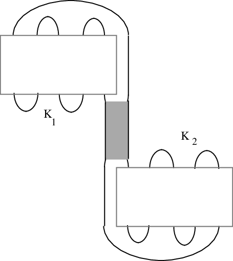
Rieck and Sedgwick [RS] show that the answer is yes when neither nor has in its exterior an essential meridional planar surface; Wu notes that their result now follows easily from Theorem 4.2. See also and [He]. Without the assumption on essential planar surfaces in the knot exteriors, only a little is currently known, e.g.
cf [ScSc], though there is strong evidence that the answer is no, cf [ST3].
5. From knots to graphs
5.1. Normal form for trivalent graphs
Thin position techniques outlined above for knots do not particularly make use of the fact that is connected (though some of the applications do) and so thin position can be applied to links as well as knots in . On the other hand, some thought is needed if thin position is to be applied to imbedded graphs in . We will restrict our discussion to trivalent graphs; presumably more general graphs can be treated similarly but so far there seems to be no notable application to higher valence graphs.
Definition 5.1.
Let be a finite trivalent graph in and let be the standard height function. is in normal form with respect to if
- (1)
the critical points of are nondegenerate and each lies in the interior of an edge;
- (2)
the critical points of and the vertices of all occur at different heights and
- (3)
At each (trivalent) vertex of either two ends of incident edges lie above (we say is a -vertex) or two ends of incident edges lie below (we say is a -vertex). (See Figure 6 a.)
Any can be perturbed by a small isotopy to be normal; for example, note that if three edges are incident to the same vertex from below, then a small isotopy moves the end of one edge so that is incident from above and has a maximum near the vertex. That is, such a vertex is replaced by an interior maximum adjacent to a -vertex. (See Figure 6 b.)

Suppose is in normal form with respect to .
Definition 5.2.
The maxima of consist of all local maxima of and all -vertices. The minima of consist of all local minima of and all -vertices.
A maximum (resp. minimum) that is not a -vertex (resp. -vertex) will be called a regular maximum (resp. minimum). The set of all maxima and minima (hence including all the vertices of ) is called the set of critical points of . The heights of the critical points are called the critical values or critical heights.
is in bridge position if there is a level sphere, called a dividing sphere, that lies above all minima of and below all maxima.
There are two sorts of complications introduced when valence vertices are allowed: there is some subtlety in finding an appropriate calculation of width; and surfaces that are properly imbedded in the graph complement may behave in a less orderly fashion. We treat each of these in turn:
5.2. Width for graphs
A naive way to define width is to proceed just as in the case of knots or links: For each generic let , a function that increases by two at a regular minimum of , and by one at a -vertex. Similarly decreases by two at a regular maximum of , and by one at a -vertex. Now pick generic heights , each between a distinct adjacent pair of critical heights, and calculate the sum . A complication that this definition introduces is this: there are now two types of maxima in , regular maxima and -vertices. If one is pushed down past the other, the width changes. In particular, if a maximum of unknown type is pushed down past other maxima and other minima, we do not a priori know that the width is decreased. (Symmetric statements are true, of course, for minima.) Such a definition then would make arguments using upper and lower disks, arguments that worked so successfully in the case of knots, pretty useless for graphs.
A fix for this is to alter the definition slightly, taking into account what the nature of the adjacent critical height is. A motivating thought is this: If we widen the graph to look like a ribbon whose core is the graph, then the boundary of the ribbon is just a standard link , with no vertices. Exchanging the heights of two critical points of will rearrange heights of several critical points on but in a predictable way. Moving maxima past maxima in will rearrange only maxima of (and so have no effect on height); moving a maximum past a minimum in will similarly move maxima past minima in . See Figure 7. It’s relatively easy to express the width of via the number of intersections of with level planes, and we will use that as the definition of the width of . The upshot is a somewhat more complicated definition, but one that automatically has the property we seek: it’s indifferent to the exchange in heights of adjacent maxima or adjacent minima, but will go down if a maximum is moved below a minimum.
Definition 5.3.
Let be the successive critical heights of . Let be generic levels chosen so that and let denote the critical point at height . For each define by:
Define the width of with respect to be
This is a essentially the width introduced in [GST, Section 3], but made symmetric with respect to reflection through a horizontal plane.

Definition 5.4.
A graph is in thin position (with respect to ) if cannot be lowered by an isotopy of . In that case, is denoted .
Remark: In practice, the chief property of the width that we will need is this: The width is decreased if a maximum is pushed below a minimum, but the width is unaffected by pushing one maximum above or below another maximum, or one minimum above or below another minimum. See Figures 7, 8.

5.3. Surfaces in graph complements
Surfaces that lie in a knot complement have the pleasant feature that boundary components are either horizontal (if the boundary component is a meridian) or the height function on the boundary circles roughly follow that of the knot, having maxima where the knot has a maximum and similarly with minima. It’s easy to locally isotope the surface so that all singularities of on its boundary are local half-centers.
In contrast, surfaces in a graph complement may have minima at -vertex maxima and maxima at -vertex minima. See Figure 9.

A graph in normal form with respect to can be thickened slightly to give a solid handlebody with the predictable height structure (e.g. very near any regular maximum of there are two non-degenerate critical points of , one a saddle just below and one a maximum just above.) We will be concerned with simple closed curves on and with properly imbedded surfaces in .
Definition 5.5.
Suppose is a graph, in normal form with respect to , and is a simple closed curve. Then is in normal form on if either it is a horizontal meridian circle or each critical point of on is non-degenerate, and occurs near an associated critical point of in . Furthermore, the number of critical points of has been minimized via isotopy of in .
Definition 5.6.
A properly imbedded surface
is in normal form if
- (1)
each critical point of on is nondegenerate,
- (2)
is in normal form with respect to
- (3)
no critical point of on int occurs near a critical height of on ,
- (4)
no two critical points of on int or occur at the same height,
- (5)
the minima (resp. maxima) of at the minima (resp. maxima) of are also local extrema of on , i.e., ‘half-center’ singularities,
- (6)
the maxima of at -vertices and the minima of at -vertices are, on the contrary, ‘half-saddle’ singularities of on .
Standard Morse theory ensures that, for in normal form, any properly imbedded surface can be properly isotoped to be in normal form.
5.4. Upper and lower triples
The definition of upper and lower disks naturally extends to the context of graphs:
Definition 5.7.
Given in normal form and a level sphere for at a generic height, let and denote the balls which are the closures of the region above and below respectively. An upper disk (resp. lower disk) for is a disk transverse to such that , where is a normal arc imbedded on , is an arc properly imbedded in , , and a small product neighborhood of in lies in (resp. ) i.e., it lies above (resp. below) .
Note that consists of simple closed curves and arcs with ends in . A natural occurence of upper (or, symmetrically, lower) disks is this: According to Definition 5.6, a maximum of near a maximum of is a half-center singularity on . In particular, a sphere just below this maximum will cut off an upper disk from .
As was noted above, curves in can be quite complicated, so a somewhat more elaborate notion than upper or lower disk will be needed.
Definition 5.8.
Suppose, as above, is in normal form and is a level sphere for at a generic height. An upper triple (resp. lower triple) for is an upper (resp. lower) disk with these properties
- (1)
The arc of Definition 5.7 has its ends at different points of (i.e. is not a loop)
- (2)
is one of the points of at an end of , and
- (3)
although there may be arc components of , none of them is incident to .
For example, in the old setting of, say, a Seifert surface for a knot , any arc of that is inessential in cuts off either an upper or a lower disk . If is either point of at the ends of , then is an upper or lower triple.
5.5. An application
As an illustration of how thin position can be used for graphs – in particular, why it is useful to have a definition that is indifferent to pushing maxima past maxima – we’ll offer an updated proof of the key Theorem in [ST1], which leads to the proof that any Heegaard splitting of is standard. (The roots of this proof go back to Otal [Ot].) For the proof in [ST1] we did not have in hand the efficient Definition 5.3 of width; instead we used a rather clumsy alternative, examining the entire function and minimizing its maximum, together with the number of times the function achieves that maximum.
The setting we consider is this: is a finite graph in normal form whose complement is -reducible, so there is a disk in which is essential in . The edges of the graph are allowed to slide over each other.
Lemma 5.9.
Suppose is a generic level sphere for , is -reducible, and the -reducing disk has been chosen to minimize and is properly isotoped to be in normal form. Then either there is an edge of that is disjoint from or there is a point with the following property: Suppose is an arc of that is outermost among the set of arcs of that are incident to . Let be the disk it cuts off from . Then is either an upper or a lower triple.
Proof.
Since was chosen to minimize it follows that every component of is essential in the planar surface . If any intersection point of with is incident to no arc component of then the edge of containing that point is disjoint from and we are done. So we may as well assume that each point of is incident to some arc component of ; it follows that some point is incident to no loops at all. Among all arcs of that are incident to , let be the arc that is outermost on . Then by construction, cuts off an upper disk (say) from in which no other arc of intersection is incident to and is not a loop in . ∎
Lemma 5.10.
Suppose the edges of have been slid and isotoped so as to minimize (cf Definition 5.3) and suppose is -reducible. Then either the edges of can be slid until there is a -reducing disk whose boundary is disjoint from an edge, or is in bridge position.
Proof.
Suppose on the contrary that is not in bridge position. Let be a thin level sphere, i. e. a level sphere intersecting so that the adjacent critical heights above and below are a minimum (possibly a -vertex) and a maximum (possibly a -vertex) respectively. Choose a -reducing disk so as to minimize . If any edge of is not incident to then we are done. If every edge is incident to then in particular is incident to every point in . In that case, let be the upper (say) triple given by Lemma 5.9. Then may be used to slide one end of the edge of on which lies down to . (The details of this move, involving possible “broken edge slides” are a bit more complicated than it might first appear, cf. [ST1, Proposition 2.2].)
Unfortunately this move, so similar to the one used in Theorem 4.4, does not in this case necessarily thin . To see why, suppose that, before the slide, the end simply ascends from into a -vertex, from below. Then the slide we’ve just described will move the end to (creating a -vertex just below and lowering by ); but also the -vertex merely becomes a regular minimum. Both the new -vertex and the transformation of the -vertex into a regular minimum will actually raise the width, by a total of . See Figure 10. This is a technical setback, but not a devastating one, as we now briefly outline.
Note that the slide we’ve just described lowers , so we cannot repeat the process indefinitely. The argument stops either because there is a -reducing disk disjoint from an edge (and we are done) or when is no longer a thin sphere. In the latter case, either all the minima above or all the maxima below have been removed by the sequence of edge slides. With no loss, assume that the process stops because all the minima above have been removed. (We do not assume that an upper disk arises at each stage, but of course an upper disk does happen to be needed at the last stage, since a lower disk would give rise to a minimum just above ). We will show that by the time the process stops, the width has been reduced.

We will assume that there are no further thin levels above and leave it to the reader to adjust the following argument for the general case (by counting for and only minima just above and then subtracting a further such term for each thin sphere above ). Let be the number of regular minima and be the number of -vertices lying above . Define
Claim: Every move in the process (whether on an upper or a lower disk) decreases .
Proof of claim: Each of the moves is either a simple isotopy of an arc of to an arc lying just above or below , or it is a slide of an end of an edge of to an arc just above or below . In the former case, no vertex moves and the proof is almost immediate. The move reduces and we only have to check that the reduction is greater than the increase of which may result from the elimination of regular minima of that lie above . These regular minima necessarily lie on the arc being isotoped. For every minimum of above there will be a maximum (and in toto one more maximum than minimum on each component of that lies above ). Eliminating both a minimum and a maximum above will reduce by a total of at least . (Since width is not altered by rearranging orders of maxima or of minima, we may assume for the purposes of calculation that the cancelling critical points are respectively the lowest maximum and the highest minimum, i.e. at adjacent heights). At the same time, will go up by only . Thus, in any case, the isotopy of will reduce .
Next suppose the move is an edge slide. If the end of an edge that is slid descends into a -vertex or ascends into a -vertex, then the edge slide does not create more critical levels and again the argument is fairly straightforward: is always reduced, and if ascends into a -vertex or if it descends into a -vertex lying below then the only minima above that disappear are internal minima for which the above argument applies. If the end of descends into a -vertex above , that minimum is eliminated (raising by ) but it can be viewed as being cancelled with an adjacent maximum, which reduces by at least .
So, not surprisingly, to prove the claim we are reduced to the case in which an extra critical level may be created, because the end either descends into a -vertex or ascends into a -vertex. (In these cases the slide does not eliminate the critical point at its end, and creates a new one near .) Let us call the terminating vertex . There are four cases: may lie above or below and the disk defining the move may be an upper or lower one. But, for example, if lies above and the disk is a lower one, we may imagine the slide as the composition of one based on an upper disk taking down below , followed by one based on a lower disk bringing back up to . In other words, it suffices to consider the two cases where lies below (resp. above) and the disk determining the slide is a lower disk (resp. upper disk).
Suppose first that is below and the move is via a lower disk, so the vertex is moved to a -vertex just above . We have already argued that eliminating internal critical points on can only improve the situation, so we may as well assume that either descends from straight down into a -vertex or has a single internal minimum, adjacent to its ascent from below into a -vertex. In the latter case the internal minimum of is also eliminated so again no new critical level is really created: In fact the slide is equivalent to a move that just brings the vertex up to . Since raising a -vertex cannot raise the width, and a new -vertex above reduces , the overall effect is to reduce . In the case where the end descends straight into , a -vertex, the slide that moves up to can be viewed as the composition of two moves: first move up to a new -vertex just above the lowest thin sphere above . We have already seen (cf. Figure 10) that this raises the width by . Next raise up above . This lowers the width every time passes a maximum: by for every -vertex passed and by for every regular maximum passed (cf. Figure 8). But then the total amount of the reduction, determined by the number and type of maxima between and is at least so in the end the move raises the width by at most . When combined with the effect of raising by , the result is that goes down by at least (indeed exactly only if ).
Finally, suppose is above and the move is via an upper disk. Again we may as well assume, because eliminating internal critical points only improve the situation, that either simply ascends from into a -vertex or its terminating end descends into a -vertex from a single adjacent internal maximum. We have seen that in the former case the width increases by exactly . On the other hand, the -vertex at becomes a regular vertex, reducing by . The net effect is to reduce by . In the latter case, again the slide effectively just moves the -vertex below , reducing the width by moving a -vertex down past minima, but having no effect on or . This finally proves the claim in all cases.
Now let be the graph when the process stops, with no further minima above . We have just seen . But since there are no minima of above , . Hence , a contradiction to the original assumption that was in thin position. ∎
Lemma 5.11.
Suppose is in bridge position and is -reducible. Then the edges of can be slid rel a dividing sphere until either
- •
there is a -reducing disk whose boundary is disjoint from an edge or
- •
for some dividing sphere there are both upper and lower triples , so that the disks are disjoint in
In the latter case, the triples may further be chosen so that either no arc of is incident to or, vice versa, no arc of is incident to .
Proof.
Let be a dividing sphere and choose among all -reducing disks for so that is minimal. In particular, this guarantees that no arc component of is a trivial loop in the planar surface .
Claim: can be slid and isotoped rel so that it is still in bridge position and at the lowest maximum (resp. the highest minimum) of , also has a maximum (resp. minimum). So for in normal form, both the lowest maximum and highest minimum of are incident to half-center singularities on .
Proof of Claim: Choose any component of , say one lying above . Since is in bridge position, is necessarily a tree. In particular, is a planar surface. If is not incident to an edge of we are done, so assume it is incident to every edge; it follows (by examining an innermost loop, if any, on the planar surface ) that there is a component of that runs from the end of one edge of to the end of another . Imagine collapsing the edges of that are not incident to to a single vertex (so is simply the cone on its ends) then sliding to recreate a trivalent graph with only maxima, in which a single pair of edges (forming a maximum that we may isotope to be the lowest maximum) contains the entire subarc of that connects to . See Figure 11. The new graph is again in bridge position and is homeomorphic to the original, so the width has not been altered. This establishes the claim.

Following the Claim, note that a level sphere just below the lowest maximum will cut off an upper disk entirely contained above the sphere; moreover the arc of intersection with is not a loop. Hence it’s an upper triple. Similarly, a level sphere just above the highest minimum will cut off a lower triple. According to Lemma 5.9 every generic level sphere in between cuts off either an upper or a lower triple. So, as usual, there is a level sphere that cuts off both an upper and a lower triple, and . Moreover at least one of the two, say , is obtained via Lemma 5.9. If, among the arcs incident to , there is also an arc cutting off a lower triple, use this triple for . Then automatically no arc of is incident to , establishing the last property required. If, on the other hand, no arc incident to cuts off a lower triple, then every arc outermost among the arcs incident to must cut off an upper triple. In this case, to establish the last property of the lemma, suppose on the contrary that some arc of is incident to . Then an outermost such arc will cut off a (possibly different) upper triple with the property that no arc of is incident to . ∎
Lemma 5.12.
Suppose is not the unknot, and the edges of have been slid and isotoped so as to minimize . Suppose further that is -reducible. Then the edges of can be further slid until there is a -reducing disk whose boundary is disjoint from an edge.
Proof.
Suppose not. Following Lemma 5.10, we may assume is in bridge position. Then consider the upper and lower triples , given by Lemma 5.11 with respect to a dividing sphere . In particular, we assume with no loss that no arc of is incident to . Then may be used to slide an end of the edge on which lies down to without affecting the end of the edge on which lies, so afterwards the latter end can also be brought to . But sliding one end down and the other end up will typically reduce the width, which is impossible. An alternate possibility is that the two moves actually level an entire edge, but again this would allow the graph to be thinned. See Figure 12 a), b). The final possibility is that the two slides together simultaneously level two edges (when and have the same pair of end vertices), moving a cycle in onto . See Figure 12 c).
If either of the disk components of is disjoint from , then either (and we are done) or that disk component is a -reducing disk as required. But even if a disk component of intersects , we can just apply to the process we earlier applied to all of to find a series of edge slides that will either finally exhibit an edge disjoint from a -reducing disk (via a point in incident to no arc of ) or will iteratively reduce the number of points in until so, as above, is a -reducing disk disjoint from an edge. ∎

Corollary 5.13.
Any Heegaard splitting of is standard.
Proof.
Given a Heegaard splitting of , let be a spine of one of the handlebodies. Apply the above argument not to just a single -reducing disk for the complement (i. e. a single meridian disk for the complementary handlebody) but to a complete collection of such disks. The argument is essentially the same and terminates either with an edge disjoint from a complete collection or with simply the unknot, i.e. the standard genus one splitting of . In the former case, a meridian circle of the edge is disjoint from a complete collection of meridians for the handlebody , so it also bounds a disk in . Thus there is a sphere in intersecting in a single point in . This is a reducing sphere for the Heegaard splitting which divides the splitting into two separate splittings of the -sphere. The conclusion follows by induction on the genus of the Heegaard splitting. ∎
6. From graphs back to knots
One might hope that thin position would be helpful in understanding the tunnel structure for knots in . We noted above that for a tunnel number one knot, thin position is bridge position. That is, if has tunnel number one and is in thin position, then there are no thin level spheres for . It’s natural to ask about the behavior of the tunnel arc with respect to the standard height function, once the knot is in thin position. The union of the knot and the tunnel arc is of course a graph in ; moreover, one way of viewing the definition of unknotting tunnel is that the graph is the spine of a genus two Heegaard splitting of . The reason that this does not just fall into the program leading to Corollary 5.13 is that in the knot tunnel case, whereas we are allowed to slide the ends of the tunnel over the knot, and over the other end of the tunnel, we can never regard a subarc of as an edge of that can be slid. Nonetheless, the answer is simple and direct: the tunnel may be made level with respect to the standard height function and this is the thinnest positioning of possible.
Theorem 6.1.
Suppose that is a knot with unknotting tunnel and is in thin position with respect to the standard height function . Then can be slid and isotoped without moving until is level – either a level arc or a level “eyeglass” (the wedge of an arc and a circle). Moreover, after is perturbed slightly (to put in normal position) the graph cannot be made thinner by sliding .
For a proof see [GST]. In fact a similar theorem is true for arbitrary genus spines of even when we do not allow edges to slide, see [ST2].
Theorem 6.1 raises the natural question whether a similar theorem is true for more than a single tunnel. In general, for a knot in , a collection of disjoint properly embedded arcs in is a system of unknotting tunnels if the graph is a Heegaard spine (i.e. the complement of is a handlebody).
Question 6.2.
Suppose is a system of unknotting tunnels for a knot , in thin position with respect to the standard height function . Suppose are slid and isotoped to minimize the width of . Is each of the tunnels a perturbed level arc?
Of course many versions of this question are possible, e. g. extending it to links or to arbitrary graphs in . Even the case of a pair of tunnels seems difficult; it seems the first order of business would need to be a generalization of Morimoto’s theorem [Mo] (so essential for the proof of Theorem [Th1]) to handlebodies of higher genus.
7. Graphs in other -manifolds
All our discussion so far revolves around objects (knots, links, graphs) in the -sphere, on which we have the standard height function. In fact, one can imagine using thin position in many other contexts. For example, if is a knot in an arbitrary closed -manifold , and is a Heegaard splitting for , one can describe the Heegaard splitting as a product structure on the complement of spines for the respective handlebodies . That is, . Just as in the applications above, one can define the width of with respect to this structure, and try to minimize the width. In effect, we are retrospectively viewing the whole discussion above as the special case in which is and the splitting is of genus . Of course, many of the arguments above rely heavily on the fact that is a sphere, so generalizing in this direction has not been particularly fruitful.
But there is a remarkable application of thin position that occurs as a crucial step in Thompson’s recognition algorithm for the -sphere [Th2]. In this section we will briefly outline how it arises, and note some related applications to other decision problems in -manifold topology.
Suppose is a closed -manifold with a given triangulation . Let be the -skeleton of the triangulation. Recall that a compact surface is normal with respect to the triangulation if
- •
is in general position with respect to (so in particular intersects is a finite number of points, each on an edge of )
- •
For each -simplex in , each component of is an arc with its ends on different faces of .
- •
For each -simplex in , each component of is either a triangle (i. e. parallel to a face of ) or a square (i. e. it is incident to each face in a single arc). See Figure 13.
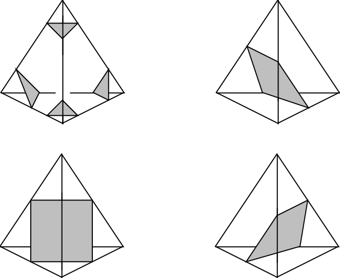
It is easy to show that any incompressible surface in can be isotoped so that it is normal. The converse is not true, most obviously because the link in of any vertex of is a normal sphere. On the other hand, if is a normal surface, then the complement is incompressible in . That implication is essentially reversible: If is a surface so that is incompressible in then may be isotoped rel so that either is normal or it’s a sphere that bounds a ball intersecting in a single unknotted arc.
There is an algorithm to find a maximal collection of disjoint non-parallel normal surfaces in ; the roots of this algorithm go back to early work of Kneser, establishing that there are at most a finite number of connected summands in [Kn]. At the very least, contains a linking sphere of each vertex, but typically there are many more. For example, if an edge of is incident to two distinct vertices, tube together their linking vertices by a tube along the edge. Unless is a specific -vertex triangulation of (cf [JR]) such a sphere is normal. In the end, it is possible to show that each component of is one of three types:
- •
a ball containing a single vertex, and bounded by a vertex-linking sphere
- •
a punctured -ball with more than one boundary component
- •
a single further component , for which .
Then is the -sphere if and only if is a -ball, and is algorithmically recognizable among the components of by the fact that it is the only component that has a single boundary component and contains no vertex. So in order to determine if is a -sphere, it suffices to find an algorithm to decide if is a -ball.
Inside of is a proper collection of arcs, and, because is incompressible in the complement of , we have that the planar surface is incompressible in . Suppose is a -ball and imagine putting in thin position with respect to the radial height function on the ball. We know immediately that is also in bridge position; that is, all the maxima lie above all the minima. For if not, consider the thin spheres in . We have noted above (essentially Theorem 4.2) that some thin sphere has the property that is incompressible in ; hence would be a normal sphere in not parallel in to . But this would contradict the completeness of .
This connection between thin spheres in and normal spheres in prompts this question: what would a thick sphere tell us? (Note that there has to be a thick sphere, since if there are only minima in then would be compressible.) If is the (unique) thick sphere, then a maximum of can be pushed down to and a minimum pushed up, but not simultaneously. Translating back into how would appear in the triangulation, it turns out that it looks just like a normal sphere, except in a single -simplex , where a single component is not a triangle or a square, but an octagon (cf. Figure 14). Such a surface is called an almost normal surface. Observe that arcs in the -skeleton of the -simplex can be pushed to the octagon from either side, but their images there necessarily intersect. Roughly the same algorithm that detects normal spheres can be used to detect almost normal spheres. The upshot is this:

Fact 1: If is the -sphere then there is an almost normal sphere in the component of .
To complete the argument that this is an algorithm, one needs to know that if there is an almost normal sphere in the component of then is not the -ball and so is not . Observe first of all that since a sub-arc of is parallel to an arc in , it follows that is compressible in on the side containing the arc: basically one constructs a compressing disk by doubling the disk defining the parallism. This argument applies on both sides of , so is compressible in in both directions (but compressing disks on opposite sides necessarily intersect). Thicken to a collar , then maximally compress in ; the result must be an incompressible planar surface (possibly with many components). Each component then just comes from a trivial sphere cutting off a ball intersecting in an unknotted arc, or it becomes a normal -sphere, hence a sphere parallel in to . Filling in all the -balls, then, creates exactly a copy of . That is, can be obtained from by attaching only and -handles to . In particular, if is a homology ball, it’s a real ball. We conclude:
Fact 2: If is a homology sphere and there is an almost normal sphere in the component of , then is the -sphere.
Since the homology of is easily calculable, the combination of Facts and gives the Thompson algorithm for recognizing the -sphere.
Without wandering too far afield, note that the algorithm above is particularly straightforward if there are few normal spheres. A triangulation (broadly defined) of a closed -manifold is -efficient if the only normal spheres are vertex linking. Clearly such a manifold must be irreducible. It is a theorem of Jaco and Rubinstein [JR] that, with just a few specific exceptions, any triangulation of a closed, orientable, irreducible -manifold can be modified to be -efficient and such a triangulation has only a single vertex. More generally, if is reducible, there is an algorithm to decompose into a connected sum of -manifolds, each of which either has a -efficient triangulation or is visibly homeomorphic to or . Thus to get an algorithm that precisely describes the connected sum decomposition of , one need only apply the Thompson algorithm above in the case in which the triangulation is -efficient.
There are other clever applications of thin position in settings that go well beyond the scope of this article. A favorite is [Lac], where Lackenby shows that the natural combinatorial ideal triangulation of a punctured torus bundle (with pseudo-Anosov monodromy) coincides with the natural hyperbolic ideal triangulation.
References
- [Al] J. W. Alexander, On the subdivision of -space by a polyhedron, Proc. Nat. Acad. Sc. 10 (1924), 6-8.
- [Ga] D. Gabai, Foliations and the topology of -manifolds. III, Jour. Diff. Geom. 26 (1987), 479–536.
- [GST] H. Goda, M. Scharlemann, A. Thompson, Levelling an unknotting tunnel Geom. Topol. 4 (2000) 243–275.
- [GL] C. McA. Gordon, J. Luecke, Knots are determined by their complements, J. Amer. Math. Soc. 2 (1989), 371–415.
- [GR] C. McA. Gordon and A. W. Reid, Tangle decompositions of tunnel number one knots and links, J. Knot Theory Ramifications 4 (1995), 389–409.
- [He] J. Hendricks, Mp-small summands increase knot width, Algebraic and Geometric Topology 4 (2004), 1041–1044.
- [JR] W. Jaco and H. Rubinstein, 0-efficient triangulations of -manifolds, J. Differential Geom. 65 (2003), 61–168.
- [Kn] H. Kneser, Geschlossene Flächen in dreidimensionalen Mannigfaltigkeiten, Jahresbericht der Deut. Math. Verein. 38 (1929), 248–260.
- [Lac] M. Lackenby, The canonical decomposition of once-punctured torus bundles, Comment. Math. Helv. 78 (2003), 363–384.
- [Lau] F. Laudenbach, Une remarque sur certains nœuds de , Compositio Math. 38 (1979), 77–82.
- [Mo] K. Morimoto, Planar surfaces in a handlebody and a theorem of Gordon-Reid, Proc. Knots ’96, ed.S.Suzuki, World Sci.Publ.Co., Singapore (1997), 127-146.
- [Ot] J.-P. Otal, Sur les scindements de Heegaard de la sphere , Topology 30 (1991) 249-258.
- [RS] Y. Rieck, E. Sedgwick, Thin position for a connected sum of small knots, Algebraic and Geometric Topology 2 (2002), 297-309.
- [ScSc] M. Scharlemann, J. Schultens, 3-manifolds with planar presentations and the width of satellite knots , to appear in Trans. Am. Math. Soc. math.GT/0304271
- [ST1] M. Scharlemann, A. Thompson, Thin position and Heegaard splittings of the -sphere J. Differential Geom. 39 (1994), 343–357.
- [ST2] M. Scharlemann, A. Thompson, Thinning genus two Heegaard spines in the 3-sphere J. Knot Theory Ramifications 12 (2003), 683–708.
- [ST3] M. Scharlemann, A. Thompson, On the additivity of knot width, in Proceedings of the Casson Fest, Geometry and Topology Monographs, 7 (2004) 135-144.
- [Schub] H. Schubert, Über eine numerische Knoteninvariante, Math. Z. 61 (1954), 245–288.
- [Schul] J. Schultens, Additivity of bridge numbers of knots, Math. Proc. Cambridge Philos. Soc. 135 (2003), 539–544.
- [Th1] Thompson, Abigail, Thin position and bridge number for knots in the -sphere, Topology 36 (1997), 505–507.
- [Th2] Thompson, Abigail, Thin position and the recognition problem for , Math. Res. Lett. 1 (1994), 613–630.
- [Wu] Y.-Q. Wu, Thin position and essential planar surfaces, Proc. Amer. Math. Soc. 132 (2004), 3417–3421.