Boundary Trace of Reflecting Brownian Motions
Abstract
We establish a uniform dimensional result for normally reflected Brownian motion (RBM) in a large class of non-smooth domains. Exact Hausdorff dimensions for the boundary occupation time and the boundary trace of RBM are given. Extensions to stable-like jump processes and to symmetric reflecting diffusions are also mentioned.
AMS Mathematics Subject Classification (2000): Primary 60G17, 60J60; Secondary 28A80, 30C35, 60G52, 60J50.
Keywords and phrases: Reflecting Brownian motion, Hausdorff dimension, uniform dimensional result, boundary occupation time, boundary trace, conformal mapping.
1 Introduction
Let and be a domain (connected open set) with compact closure. Consider a reflecting Brownian motion (RBM in abbreviation) in . Heuristically, RBM in is a continuous Markov process taking values in that behaves like a Brownian motion in when and is instantaneously pushed back along the inward normal direction when . RBM on smooth domains can be constructed in various ways, including the deterministic Skorokhod problem method, stochastic differential equation with boundary condition, martingale problem methods, etc. see the Introduction of [6]. When is non-smooth, all the above mentioned methods cease to work. On non-smooth domains, the most effective way to construct RBM is to use the Dirichlet form method, which will be recalled in Section 2. The RBM constructed through Dirichlet form coincides with all the other standard definitions in smooth domains. Using the Dirichlet form approach, it can be shown that, when is a simply connected planar domain, RBM in is the time change of the conformal image of RBM in a unit disc.
This paper is concerned with Hausdorff dimensions of various random sets associated with RBM. The study of Hausdorff dimensions of random sets associated with Brownian motion, stable processes and more generally Lévy processes together with their fractal structures has been an active research area in the last 40 years. See Xiao [30] for a recent survey on this subject. However, to the authors’ knowledge, this is the first time that such a study has been conducted for RBM in Euclidean domains.
The results obtained in this paper hold for a large class of non-smooth domains. In order to convey our results as transparently as possible, in this introductory section we confine ourselves to a special case of the more general results established in this paper by assuming that is a bounded uniform domain. The following definition is taken from Väisälä [29], where various equivalent definitions are discussed.
Definition 1.1
A domain is called uniform if there exists a constant such that for every there is a rectifiable curve joining and in with and moreover for all points . Here is the Euclidean distance between point and the set .
For example, the classical van Koch snowflake domain in the conformal mapping theory is a uniform domain in . The uniform domain is also called -domain in the terminology of Jones [17]. Note that every Lipschitz domain is uniform, and every non-tangentially accessible domain defined by Jerison and Kenig in [18] is a uniform domain (see (3.4) of [18]). However, the boundary of a uniform domain can be highly nonrectifiable and, in general, no regularity of its boundary can be inferred (besides the easy fact that the Hausdorff dimension of the boundary is strictly less than ). For any , one can construct a uniform domain such that for any open set satisfying . Here denotes the -dimensional Hausdorff measure in .
In this paper, we first extend Kaufman’s uniform doubling dimension result [20] for planar Brownian motion to RBMs in bounded domains. It follows as a special case of Theorem 3.1 below that for RBM in a bounded uniform domain ,
| (1.1) |
Here denotes the range of under RBM and denotes the Hausdorff dimension. Such a result is called a uniform dimensional result because the exceptional set in (1.1) is independent of the Borel time sets . This dependence is important when one wants to extract information on by observing only while itself is random, for example, when is the boundary occupation time set of .
We next study the occupation time of on the boundary ,
Corollary 4.3 below implies that
| (1.2) |
-almost surely for every . Note that for any Euclidean domain , . This together with (1.1) implies that the Hausdorff dimension of the boundary trace for RBM in is
-almost surely for every . In particular, for planar uniform domains (such as the van Koch snowflake) it follows that -almost surely
for every . This is in contrast to Makarov’s celebrated result about the support of harmonic measure: There is a subset of with such that the first intersection of with is almost surely contained in . In Section 5 an example of a (non-uniform) domain is given where the Hausdorff dimension of the boundary trace of RBM in differs from . Thus some assumption about the regularity of the domain is necessary for our results to hold.
The remainder of this paper is organized as follows. In Section 2, we recall the definitions of RBM and extension domains. In Section 3, we show that the sample paths of RBM have the same degree of Hölder continuity as Brownian motion, by using the Lyons-Zheng’s forward-backward martingale decomposition of RBM. We then establish the uniform dimensional results for RBM on a large class of non-smooth Euclidean domains. For this we derive the two-sided heat kernel estimates for RBM and use a capacitary argument. In the case of dimension , the logarithmic capacity is not good for our approach so we first subordinate the RBM, then establish dimensional results for the subordinated stable-like process and lastly transfer these results back to RBM. In this procedure, we use the recently obtained two-sided heat kernel estimates in Chen and Kumagai [7] for stable-like processes on . In Section 4, we apply a recent result in Bogdan, Burdzy and Chen [4] to get the exact capacitary dimension of the boundary occupation time of RBM and therefore establish its Hausdorff dimension. All these results are combined in Section 5 to get the Hausdorff dimension for the boundary trace of RBM. Several examples are given to illustrate the main results of this paper as well as an example that shows that certain regularity assumptions on the domain are needed for the main results of this paper to hold. Extensions of the main results in this paper to stable-like jump processes are mentioned in Remarks 3.10, 4.4 and 5.2.
We point out here that the approach used in this paper is quite robust that applies not only to RBM but also to symmetric reflecting diffusions as well. These symmetric reflecting diffusions have infinitesimal generators of divergence form:
where is a symmetric matrix-valued measurable function that is uniformly elliptic and bounded. See Chen [6] for relevant informations on symmetric reflecting diffusions on bounded domains, and Stroock [28] for two-sided heat kernel estimates for symmetric diffusions on .
2 Extension domains and RBM
Throughout this paper, is an integer. For a domain , let , equipped with the Sobolev norm , where . In this paper we will be concerned with reflecting Brownian motion on domains whose boundary has zero Lebesgue measure and have the following -extension property: there is a bounded linear extension operator
| (2.1) |
The -domains (also called locally uniform domains) introduced by P. W. Jones [17] have this property. A domain is , if there are and such that the conditions in Definition 1.1 for uniform domains hold for with . Clearly, an -domain is just a uniform domain. For later use, we record the following observation as a lemma.
Lemma 2.1
If is an -domain, then so is .
Proof. If with , then either or . In the first case, we can easily lift the rectifiable curve from to in in the definition of -domain for to a rectifiable curve from to that satisfies the -condition for , with possibly different values of and . In the second case, we construct a point with such that , and then apply the first case to construct rectifiable curves joining with and with . The piecing together curve satisfies the condition for -domain for , with possibly different values of and .
The importance of -domains is further illustrated by the following. It is shown by Jones [17] that a finitely connected domain is a -extension domain if and only if it is an -domain. More information on domains that have the -extension property (2.1) can be found in Herron and Koskela [15].
For , define
and . We say the Dirichlet form is regular on if is dense both in and in . It is known (cf. Theorem 2 on p.14 in Maz’ja [24]) that is a regular Dirichlet form on if has continuous boundary. Clearly is a regular Dirichlet form on . So if is a -extension domain, is regular on .
When is regular on , there is a strong Markov process associated with , having continuous sample paths on ; one can construct a consistent Markovian family of distributions for the process starting from every point in except possibly for a subset of having zero capacity (see Chen [6]). When is smooth, the exceptional set can be taken to be the empty set. We will show in Section 3 (see (3.6) and Lemma 3.7 below) that the exceptional set in fact can be taken to be the empty set for a large class of nonsmooth domains including -domains. Thus constructed process is the reflecting Brownian motion on in the sense that this definition agrees with all other standard definitions in smooth domains. As it is remarked in Bass, Burdzy and Chen [2] (see the second paragraph in the proof of Theorem 5.7 there), such reflecting Brownian is conformally invariant on planar domains.
Let be the occupation time of on the boundary and the trace of on the boundary .
Recall that for any increasing function on with , one can define a Hausdorff measure with respect to the gauge in the following way (see, e.g., p.132 of [1]). For ,
| (2.2) |
When for some , the Hausdorff measure will be denoted as .
Definition 2.2
A Borel set is called an -set if there exists a positive constant such that
where denotes the Lebesgue measure in .
3 Uniform Dimensional Results for RBM
In this section, we will extend Kaufman’s uniform dimensional result for planar Brownian motion to reflecting Brownian motions in -dimensional bounded domains. This is perhaps the first time such a uniform dimensional result has been established for a recurrent Markov process that does not have the property of independent increments.
Theorem 3.1
We will prove the upper bound first.
Theorem 3.2
Proof. We first show that the sample paths of RBM have the same degree of Hölder continuity as Brownian motion. Clearly, since RBM behaves like Brownian motion when , the sample paths of can not be smoother than those of Brownian motion. By Lyons-Zheng’s forward and backward martingale decomposition (see Theorem 5.7.1 of Fukushima, Oshima and Takeda [11]), for any ,
| (3.3) |
where is a martingale additive functional of which is an -dimensional Brownian motion, and is the time reversal operator of at time , i.e., for each . Since is symmetric under , is invariant under time reversal . For , define
It follows from (3.3) that q.e. on . Here q.e. is the abbreviation for quasi-everywhere; that is the above property holds holds for every point in except a set of zero capacity with respect to the RBM . Since is finely continuous, we have q.e. on . This implies that for q.e. ,
Taking a sequence , we have for q.e. ,
Since has density function for every (see Fukushima [10]), the above holds for every . If satisfies the condition of Theorem 3.1, then by (3.6) and Lemma 3.7 below, has transition density function for every . It follows that (3.2) holds for every .
Remark 3.3
In fact, Theorem 3.2(i) holds for RBM on any Euclidean domain, with the same proof. See Chen [6] for the construction of RBM and its forward-backward martingale decomposition on an arbitrary Euclidean domain. When is a domain satisfies the condition of Theorem 3.1, (3.2) can also be established by using the heat kernel estimates obtained in (3.6) and Lemma 3.7 together with a result initially due to Hawkes and Pruitt (see Lemma 8.1 of Xiao [30].
To prove the lower bound in Theorem 3.1, we treat the higher dimensional case () and two-dimensional case separately.
Let be a domain that satisfies the condition of Theorem 3.1. Let be a Borel set of having zero capacity with respect to RBM in such that for every ,
Such a set is called a properly exceptional set of and alway exists (see [11]). When , by the classical Sobolev inequality on and (2.1),
| (3.4) |
Thus according to Varopoulos (see Theorem 2.4.2 in Davies [8]) the reflecting Brownian motion has density function such that
| (3.5) |
Recall that it is assumed that has zero Lebesgue measure. Using Davies’ method together with an old idea of Nash advanced by Fabes and Stroock in [9], it is now standard to deduce that (cf. Theorem 2.3 and Theorem 3.4 in [3] and Section 3 in [9]) is jointly Hölder continuous on and for any there are positive constants and such that
| (3.6) |
for and . So can be extended continuously to . This in particular implies that reflecting Brownian motion on a -extension domain with can be constructed as a strong Markov process that starts from every point in (cf. [11]).
The following covering lemma was first proved for Lévy processes in by Pruitt and Taylor [27]. It is extended to general Markov processes in Liu and Xiao [22].
Lemma 3.4
Let be a collection of cubes of side in with the property that the number of these cubes which intersect an arbitrary sphere of radius in is bounded by a constant that is independent of and of the sphere (this happens when the cubes are those in or when the cubes do not overlap too much). Let satisfy the condition of Theorem 3.1 and let be the number of those cubes that are hit by RBM in before time . Then there is a constant that depends only on and such that
| (3.7) |
for every .
It follows from (3.6) that
| (3.8) |
Lemma 3.5
If is a ball of radius in and , then there is a constant such that
for every and .
Proof. Let be the 1-equilibrium measure of for ; that is,
where and . Note that
It follows from the extension property (2.1) that , where and denote the 1-capacity of for RBM on and Brownian motion in , respectively. Hence
which proves the lemma.
.
Theorem 3.6
Suppose that , that is a bounded domain satisfying the extension property (2.1) and that has Lebesgue measure. Then for every ,
| (3.9) |
Proof. With Lemmas 3.4 and 3.5 in hand, by the same argument as those for Lemma 3 and Theorem 1 in Hawkes [13], we have
for every and . Letting , we see that (3.9) holds for every .
So far we have proved Theorem 3.1(1). In the remainder of this section, we will deal with the two-dimensional case.
Lemma 3.7
Suppose is a bounded domain whose boundary has zero Lebesgue measure such that is a -extension domain in . Then reflecting Brownian motion on exists as a strong Markov process on starting from every point in . Furthermore its transition density function is jointly Hölder continuous on and has Gaussian estimates (3.6) with there.
Proof. Under the assumptions of the lemma, is a -extension domain in so RBM on exists as a strong Markov process on starting from every point in except on a properly exceptional set of . Note that RBM in can be obtained from by running an independent RBM in the unit interval along the -direction. By (3.5), RBM on has transition density function and
It follows that has density function and that
Joint Hölder continuity of and its two-sided estimate (3.6) (with ) now follows from a similar argument as that in Section 3 in Fabes and Stroock [9] and that for Theorems 2.3 and 3.4 in Bass and Hsu [3]. So the RBM can be refined to start from every point in .
Remark 3.8
By Lemma 2.1 and the remark at the end of Section 2, any bounded planar -domain satisfies the condition of Lemma 3.7. Combining this with a result of Jones mentioned at the paragraph following Lemma 2.1, we see that any bounded finitely connected -extension domain in satisfies the condition of Lemma 3.7.
Theorem 3.9
Proof. Let be a reflecting Brownian motion in with sample space . By Lemma 3.7, the transition density function has the estimate (3.6) with . For , let be a -valued process on a probability space with independent increments such that
We assume that and are independent and live on a common probability space. This can be achieved on the product space with product measures . Define ; that is, is the -subordinate of .
It follows from Kumagai [21] that is a special case of the stable-like processes on studied in Chen and Kumagai [7]. Hence by Theorem 1.1 of [7] the transition density function of has the property that
and
| (3.10) |
on any finite time intervals. Here for two function , means there are two positive constants such that . Furthermore, it follows from Theorem 2.5(1) and its proof in Bogdan, Burdzy and Chen [4] that the capacity induced by on is controlled by the capacity induced by the symmetric -stable process in (cf. also Lemma 3.1 of Fukushima and Uemura [12]). Thus by a similar argument as that for Lemma 3.5 above, we have
where is a ball of radius in , , and is a constant that depends only on , and . Using this and applying Lemma 3.4 to the process , the same reasoning as that in the proof of Theorem 3.6 implies that for every ,
| (3.11) |
For a Borel set , define . Clearly , and the random number depends only on the subordinator and , which is independent of and therefore of . Thus by (3.11) and Fubini’s theorem, for every , there is with such that for every and for every Borel measurable set ,
| (3.12) |
Thus for every and every Borel measurable set ,
which by (3.8) of Pruitt [26] is no less than . Hence we have shown that for every ,
Letting proves the theorem.
Remark 3.10
Let be a closed set such that there are constants and so that for every ,
(such a set is called a -set). Let be an -stable-like process on (see Chen and Kumagai [7] for the definition), where and . It is shown in [7] that has a jointly Hölder continuous transition density function on and that
on for every . Using a similar argument as above, one can show that
As it is observed by Xiao in [30], applying a result initially due to Hawkes and Pruitt (see Lemma 8.1 of [30]), one gets
Hence we have for and ,
| (3.13) |
Taking , one can see clearly that the above can not be true when .
4 Boundary Occupation Time
Theorem 4.1
Suppose that is a bounded open -set satisfying condition (2.1). Then for ,
-
(i) -a.s. for every if is polar for the symmetric -stable process in .
-
(ii) -a.s. for every if is not polar for the symmetric -stable process in .
Proof. For , let be the -subordinator that is independent of RBM in . Then is a recurrent symmetric Markov process with density functions and its associated Dirichlet form has the property that its -norm is comparable to the Besov norm in (see Kumagai [21] for a calculation). Hence by Theorem 2.5 in Bogdan, Burdzy and Chen [4], is polar for if and only if it is polar for the symmetric -stable process in . Note that according to Frostman the Hausdorff dimension is the same as the Riesz capacitary dimension, while Orey showed that one-dimensional -stable processes share the same polar sets (see Lemma 2 in Hawkes [14]). Therefore we have for any Borel set ,
So for every , -a.s.,
This proves the theorem.
The above theorem implies that almost surely if and only if is polar for symmetric -stable process in with and non-polar for symmetric -stable process with .
Remark 4.2
There is an intimate relationship between the Hausdorff measure (see (2.2) for its definition) and the Riesz capacity of order , see Theorems 2.2.7, 5.1.9 and 5.1.13 in [1]. Namely, implies that . On the other hand if then for every such that
| (4.1) |
In particular, implies for any . Later we will use the fact that for and implies , where stands for the logarithmic capacity see Theorem 5.1.9 in [1].
Recall that for any Euclidean domain , . Combining Remark 4.2 with Theorem 4.1, we have the following corollary.
Corollary 4.3
Suppose that is a bounded open -set satisfying condition (2.1). Then -a.s. for every .
Proof. If for some , for an increasing sequence of Borel sets such that , then by Remark 4.2, and so almost surely. If for some , then and hence almost surely. Since
the conclusion of the corollary now follows.
Remark 4.4
Let be an -stable-like process on an open -set in the sense of Chen and Kumagai [7]. It includes as a special case the reflected -stable process on introduced in Bogdan, Burdzy and Chen [4]. A similar argument gives the Hausdorff dimension of the boundary occupation time for , which asserts that -almost surely
for every . Hence we have for every , -a.s.
| (4.2) |
Note that when has locally finite -dimensional Hausdorff measure for , it follows from [4] that is a polar set for and therefore is the empty set almost surely.
5 Boundary Trace of RBM
Theorem 5.1
Let with be a bounded connected -set satisfying the condition of Theorem 3.1. Then the Hausdorff dimension for the boundary trace of RBM in is
for every .
Remark 5.2
Example 5.3 Let with be a bounded Lipschitz domain. Then it is an -set, satisfies the condition of Theorem 3.1, and . So the boundary occupation time set and boundary trace of RBM in have Hausdorff dimensions and , -a.s., respectively, for every .
Example 5.4 Let be a van Koch snowflake domain. By Remark 3.8 it satisfies the condition of Theorem 3.1(2) and it is well known that has Hausdorff dimension . Hence by Theorem 5.1 the boundary occupation time set and the boundary trace of RBM in have Hausdorff dimensions and -a.s., respectively, for every .
Example 5.5 Let , where is the van Koch snowflake domain in . Then satisfies the condition of Theorem 3.1(1) and . Hence by Theorem 5.1 the boundary occupation time set and the boundary trace of RBM in have Hausdorff dimensions and -a.s., respectively, for every . Note that the reflecting Brownian motion in is , where is the RBM in and is the RBM in . The above boundary trace result may be a bit surprising if one compares it with the range and the graph of a 1-dimensional Brownian motion . It is known that the Hausdorff dimension for the range of is 1 a.s., while the Hausdorff dimension for the graph of is a.s.
Example 5.6 Generalizing Example 5.4, let be a simply connected domain whose boundary is a regular fractal in the sense of [23] (the typical examples are from complex dynamics, namely components of the Fatou set of a hyperbolic rational function, and self-similar curves such as the van Koch snowflake). It is well-known that has positive and finite -dimensional Hausdorff measure, where By Theorem 5.1 the boundary trace of RBM in has Hausdorff dimension almost surely. We will now outline an alternative proof of this result, based on complex analytic methods. Let be a conformal map of the unit disc onto . Using the methods and results from [23], Section 3 (in particular Proposition 3.2), one can show that there is a set with such that
| (5.1) |
In fact, one can show that there is such that the set
satisfies , and that is uniformly expanding on
for every and all . This easily implies that satisfies (5.1). By conformal invariance is a time change of RBM in . Therefore has the same law as the boundary trace of RBM in . Because RBM in can be constructed from 2-dimensional Brownian motion by reflecting the part outside , and because Brownian motion intersects in a set of dimension almost surely by [25], we obtain a.s. Now (5.1) implies almost surely.
Example 5.7 Our final example shows that some assumption on the regularity of has to be made in order for Theorem 5.1 to hold. We will construct a simply connected planar domain such that
where has -finite length, has positive area, and has zero logarithmic capacity, where is a conformal map. Thus planar Brownian motion does not visit . Using conformal invariance as in Example 5.6, it follows that and hence a.s., while .
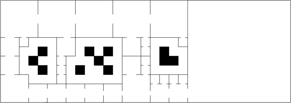
The idea is to construct as a countable union of “smooth” domains, for instance squares, joined by narrow “corridors”. The limit set of the squares is , and the width of the corridors can be arranged so that , where denotes logarithmic capacity of a set . To give a rigorous description, it is easier to begin with the set : Let be a totally disconnected compact set of positive area in the unit ball . Consider a decomposition
by closed squares with pairwise disjoint interiors, for instance the Whitney decomposition of It is easy to find line segments such that each is contained in some edge of some and such that
is connected and simply connected, see Figure 1. Then where has -finite length. Let denote the length of and a conformal map. Since is locally connected, extends continuously to . Given any sequence it is easy to choose the such that for all (for instance using Beurling’s projection theorem, which gives ). Denote the arc on that is separated from 0 by , so that If then passes through infinitely many Therefore for all By choosing such that we get with Now follows from Remark 4.2.
Acknowledgements. We thank Y. Xiao for very helpful comments on a preliminary version of this paper.
References
- [1] D. R. Adams and L. I. Hedberg, Function Spaces and Potential Theory. Springer, 1996.
- [2] R. F. Bass, K. Burdzy and Z.-Q. Chen, Uniqueness for reflecting Brownian motion in lip domains. Preprint, 2002.
- [3] R. F. Bass and P. Hsu, Some potential theory for reflecting Brownian motion in Hölder and Lipschitz domains. Ann. Probab. 19 (1991, 486-508.
- [4] K. Bogdan, K. Burdzy and Z.-Q. Chen, Censored stable processes. To appear in Probab. Theory Relat. Fields.
- [5] K. Burdzy and Z.-Q. Chen, Coalesence of synchronous couplings. Probab. Theory Relat. Fields 123 (2002), 553-578.
- [6] Z.-Q. Chen, On reflecting diffusion processes and Skorokhod decompositions. Probab. Theory Relat. Fields, 94 (1993), 281-351.
- [7] Z.-Q. Chen and T. Kumagai, Heat kernel estimates for stable-like processes on -sets. To appear in Stochastic Process Appl.
- [8] E. B. Davies, Heat Kernels and Spectral Theory. Cambridge Univ. Press, 1989.
- [9] E. B. Fabes and D. W. Stroock, A new proof of Moser’s parabolic Harnack inequality using the old ideas of Nash. Arch. Rational Mech. Anal. 96 (1986), 327-338.
- [10] M. Fukushima, A construction of reflecting barrier Brownian motions for bounded domains. Osaka J. Math., 4 (1967), 183-215.
- [11] M. Fukushima, Y. Oshima and M. Takeda, Dirichlet Forms and Symmetric Markov Processes. Walter de Gruyter, Berlin, 1994
- [12] M. Fukushima and T. Uemura, On Sobolev and capacitary inequalities for contractive Besov spaces over -sets. To appear in Potential Analysis.
- [13] J. Hawkes, Some dimension theorems for the sample function of stable processes. Indiana Univ. Math. J. 20 (1971), 733-738.
- [14] J. Hawkes, On the Hausdorff dimension of the intersection of the range of a stable process with a Borel set. Z. Wahrsch. 19 (1971), 90-102.
- [15] D. A. Herron and P. Koskela, Uniform, Sobolev extension and quasiconformal circle domains. J. D’Anal. Math. 57 (1991), 172-202.
- [16] N. Jacob and R. Schilling, Some Dirichlet spaces obtained by subordinate reflected diffusions. Rev. Mat. Iberoamericana 15 (1999), 59–91.
- [17] P. W. Jones, Quasiconformal mappings and extendability of functions in Sobolev spaces. Acta Math. 147 (1981), 71-88.
- [18] D. Jerison and C. Kenig, Boundary behavior of harmonic functions in nontangentially accessible domains. Adv. in Math. 46 (1982), 80–147.
- [19] A. Jonsson and H. Wallin, Function Spaces on Subsets of . Mathematical Reports, Vol. 2, Part 1. Acad. Publ., Harwood, 1984.
- [20] R. Kaufman, Une propriété métrique du mouvement brownien. R. Cad. Sc. Paris, 268 (1969), 727-728.
- [21] T. Kumagai, Some remarks for jump processes on fractals. To appear in Proc. of the Conference held in Graz 2001, Birkhäuser.
- [22] L. Liu and Y. Xiao, Hausdorff dimension theorem for self-similar Markov processes. Probab. Math. Statist. 18 (1998), 369-383.
- [23] N. Makarov, Fine structure of Harmonic measure. Algebra i Analiz 10 (1998), 1-62; translation in St. Petersburg Math. J. 10 (1999), 217-268.
- [24] V. G. Maz’ja, Sobolev Spaces. Springer, Berlin-Heidelberg, 1985.
- [25] Y. Peres, Intersection-equivalence of Brownian paths and certain branching processes. Comm. Math. Phys. 177 (1996), 417-434.
- [26] W. E. Pruitt, Some dimension results for processes with independent increments. In “Stochastic Processes and Related Topics, Vol. 1”, ed. M. L. Puri, Academic Press, 1975.
- [27] W. E. Pruitt and S. J. Taylor, Sample path properties of processes with stable components. Z. Wahrsch. verw. Gebiete 12 (1969), 267-289.
- [28] D. W. Stroock, Diffusion semigroups corresponding to uniformly elliptic divergence form operators. Séminaire de Probabilités, XXII, 316-347, Lecture Notes in Math., 1321, Springer, Berlin, 1988.
- [29] J. Väisälä, Uniform domains. Tohoku Math. J. 40 (1988), 101-118.
- [30] Y. Xiao, Random fractals and Markov processes. Preprint, 2002.
Itai Benjamini
Weizmann Institute, Rehovot 76100, Israel
Email: itai@wisdom.weizmann.ac.il
Zhen-Qing Chen and Steffen Rohde
Department of Mathematics, University of Washington, Seattle, WA 98195, USA
E-mail: zchen@math.washington.edu and rohde@math.washington.edu