A Contamination Carrying Criterion for Branched Surfaces

Let $M$ be an oriented 3-manifold and let $B\hookrightarrow M$ be a closed branched surface embedded in $M$. A contamination carried by B (which will be defined precisely later) is a plane field defined on a certain kind of regular neighborhood of $B$. In fact, we shall use two different kinds of neighborhoods of branched surfaces. Let $N(B)$ denote a fibered neighborhood of the branched surface $B$. It is foliated by interval “fibers” and its boundary is decomposed into two parts: the vertical boundary $\partial_{v}N(B)$ and the horizontal boundary $\partial_{h}N(B)$, see Figure 1. There is a projection $\pi:N(B)\to B$ which collapses the interval fibers foliating $N(B)$. The branched surfaces used in this paper have generic branch locus, meaning that the branched surface is locally modelled on the branched surfaces shown in Figure 1. Definitions related to branched surfaces can be found in [7], [2], [5], [3], and [4]. If we collapse the interval fibers of $\partial_{v}N(B)$, then we obtain another type of neighborhood, $V(B)$ as shown in Figure 1. Corresponding to $\partial_{v}(N(B))$, which is a union of annuli, we have $\partial_{v}(V(B))$, which is a union of curves. Again we have a projection, also denoted $\pi$, which projects $V(B)$ to $B$, $\pi:V(B)\to B$, and which projects $\partial_{v}V(B)$ to the branch locus of $B$. Cutting $\partial V(B)$ on the curves of $\partial_{v}V(B)$, we obtain the horizontal boundary, $\partial_{h}V(B)$ which is smoothly mapped to $M$.

A positive contamination $\xi$ carried by $B$ is a smooth plane field defined on $V(B)$ which is everywhere transverse to fibers of $V(B)$, is a positive confoliation in $\text{int}(V(B))$, and is tangent to $\partial_{h}V(B)$. A negative contamination is defined similarly. A pure positive contamination carried by $B$ is a positive contamination which is contact in $\text{int}(V(B))$.

For the following definition it will be convenient to choose a Riemannian metric on a given generic branched surface $B$ such that branch curves intersect orthogonally. A positive twisted immersed surface of contact for $B$ is an immersion $f:F\to N(B)$ mapping an oriented surface $F$ transverse to fibers of $N(B)$ except possibly at $\partial F$. The map $f$ restricted to $\partial F$ must map $\partial F$ transverse to fibers in $\text{int}(\partial_{v}N(B))$ except possibly on finitely many closed disjoint intervals $C_{1},C_{2},\ldots,C_{k}$ in $\partial F$, which are embedded by $f$ in fibers of $N(B)$ corresponding to double points of the branch locus of $B$. We also require that $f(C_{i})$ intersect $\text{int}(N(B))$, i.e. are not contained in $\partial_{v}N(B)$. We let $C=\cup_{i}C_{i}$, and we say that each $C_{i}$ is a corner. The immersion must satisfy further conditions. We can pull back the fibered neighborhood structure to $F$ obtaining $N_{F}$, a portion of a fibered neighborhood over $F$, see Figure 2, homotopically equivalent to $F$. The orientation on $F$ and an orientation on $N_{F}$ determine an orientation on fibers of $N_{F}$. We require that $f$ embed each oriented $C_{i}$ to a fiber respecting orientations: The orientation induced on $\partial F$ by the orientation on $F$ also gives an orientation for $C$, and $C$ must be mapped to $N_{F}$ such that the oriented arcs are mapped respecting orientation to the oriented arcs of $N_{F}$. For example, in Figure 2, $N_{F}$ is shown for an immersed disk of contact $F$, and the orientation on $F$ induces the upward orientation on fibers of $N_{F}$. We see in the figure, that the orientation on $C_{i}$’s induced by the orientation of $F$ are the same as the orientations induced by the orientations of fibers of $N_{F}$. There are more requirements. The map $\pi\circ f$ descends to a map (also denoted $f$) on the quotient space $F/C$, in which each arc $C_{i}$ becomes a point which we call a corner. Pulling back the metric of $B$ to $F/\sim$ using the map $f:F/C\to B$, we require that at its corners $F/\sim$ have interior angles $\pi/2+2n\pi$ for some $n\geq 0$. If $C=\emptyset$, then we say $f$ is an immersed surface of contact, but not a twisted immersed surface of contact; thus, for a twisted immersed surface of contact we require $C\neq\emptyset$.

A negative twisted immersed surface of contact is defined like the positive one, but now $C_{i}$’s are mapped to interval fibers corresponding to double points of the branch locus of $B$ reversing orientations.

If the map $f:F/C\to B$ is an embedding, it is easy to draw the embedded twisted surface of contact as it appears in $B$. We illustrate a positive embedded twisted disk of contact in Figure 3. The figure includes a schematic representation obtained by viewing the branch locus from “above,” where above is defined in terms of the transverse orientation of the disk. Of course, giving the disk the opposite orientation still gives a positive twisted disk of contact of the same sign. In the schematic representation of a portion of branched surface, one also needs to indicate the direction of branching. If sectors $W,X,Y$ are adjacent along an arc of branch locus $\gamma$, and if $W\cup Y$ and $X\cup Y$ are smooth, we say that branching along the arc $\gamma\subset\partial Y$ is inward for $Y$ and that branching along the arc $\gamma\subset\partial X$ is outward for $X$. We indicate the inward direction with an arrow as shown in Figure 3.

We should point out that Figure 3 is somewhat misleading, in that the behavior at the boundary of a twisted immersed surface of contact can be worse than illustrated. Namely, at a corner $c_{i}$ of $F/C$, the image of $F/C$ under $f$ may wrap around $f(c_{i})$ (a double point of the branch locus of $B$) more than one full turn, so that $f$ is not even locally an embedding in a neighborhood of $c_{i}\in F/C$. This is described in Section 2, see Figure 4.

The name “positive twisted immersed surface of contact” is too long, so we reluctantly resort to the use of an acronym. A tisc is a twisted immersed surface of contact; a positive tisc is a positive immersed twisted surface of contact; an isc is an immersed surface of contact.

Open sectors of a branched surface $B$ are the connected components obtained after removing the branched locus from $B$; sectors are their completions relative to a Riemannian metric on the branched surface. A positive (negative) tisc for $B$ induces integer weights on the sectors. If $f:F\to N(B)$ is a tisc, the weight on a given sector is the number of components in the tisc of the preimage of the open sector under the map $\pi\circ f$. The weights assigned to all sectors give the weight vector. These weights must satisfy certain equations and inequalities, called positive (negative) tisc equations and inequalities which we shall describe in Section 2. There are similar weight vectors for immersed surfaces of contact, which satisfy other relations called isc equations and inequalities.

The proof of Theorem 1.1 occupies Sections 3-7. It is preceded (in Section 2) by a discussion of weights and the proof of Theorem 1.2 as a corollary to Theorem 1.1.

In this section we discuss weight vectors induced by tiscs and iscs and prove Theorem 1.2, assuming Theorem 1.1.

As we mentioned in the introduction, a tisc can locally be more complex near a corner than shown in Figure 4a. In general, a tisc can be locally embedded in $N(B)$ as a truncated helix near an interval fiber of $N(B)$ which is the preimage of a double point of the branch locus, see Figure 4b. The figure shows a helical surface rotating between 1 and 2 full turns; in general, any number of full turns can be added. With a particular Riemannian metric on $B$ such that branch curves all intersect orthogonally, the angle of rotation after projecting to $B$ is $\pi/2+2n\pi$ for some $n\geq 0$, and in the figure the angle is $5\pi/2$. If a tisc has a corner with angle $\pi/2+2n\pi$, $n>0$, on its boundary, it cannot easily be represented using the schematic of Figure 4a. However, we shall see that an arbitrary tisc can be replaced by one with “convex” or $\pi/2$ corners only, and having the same weight vector. Formally, if $f:F\to N(B)$ is a tisc, a convex corner is a corner of the surface $F/C$ such that $f:F/C\to B$ is locally an embedding near this point.

In order to describe a practical method for detecting tiscs in a branched surface $B\hookrightarrow M$, we will describe the weight vectors induced by tiscs. If a branched surface has no weight vectors of this kind, we will conclude that $B$ has no tiscs. In a generic branched surface $B\hookrightarrow M$, there are two kinds of double points of the branch locus, as shown in Figure 5. A positive (negative) double point is of the kind that lies on the boundary of a positive (negative) tisc. Looking at the negative double point of Figure 5, we can describe the integer weight vectors corresponding to a negative tisc $f:F\to N(B)$. For each arc or closed curve of the branch locus with double points removed, the weights must satisfy inequalities like $z\geq x+y$, called a branch curve inequality. For this inequality, the curve of the branch locus in question is an arc or closed curve common to the boundaries of the sectors labelled $x,\ y,\ z$ respectively. In the figure, we also have branch curve inequalities $z\geq w+v$, $v\geq u+y$, and $x\geq w+u$. Each inequality is strict if a portion of $\partial F$ is mapped by $\pi\circ f$ to the edge corresponding to the inequality. The boundary of a positive tisc cannot turn the corner at a negative double point, so for a positive tisc, we would also have the corner equation

For a negative tisc, there are similar equations at positive double points. For a negative tisc at a negative double point, we have a corner inequality

Finally, for a negative tisc there must exist a double point where the above inequality is strict. Of course, all weights must be $\geq 0$. The equations and inequalities satisfied by weight vectors induced by a negative (positive) tisc will be referred to as the negative (positive) tisc equations and inequalities. An integer weight vector satisfying these equations and inequalities is called a negative (positive) tisc weight vector.

Similarly, an immersed surface of contact or isc, connected or not, determines an isc weight vector (with at least one curve inequality strict and all corner equations satisfied). The equations and inequalites satisfied by weights induced by an isc are called isc equations and inequalities. An integer weight vector satisfying these equations and inequalities is called an isc weight vector.

One might then ask whether a negative (positive) tisc weight vector determines a tisc $f:F\to N(B)$ embedded in $N(B)$, but with $f:F/C\to B$ possibly not an embedding. (Recall that invariant weight vectors, which satisfy all switch equations, uniquely determine measured laminations carried by $B$, and uniquely determine surfaces carried by $B$ if all weights are non-negative integers.)

The proof of Theorem 1.1 occupies Sections 3-7. Its first essential part (described in Section 4) consists of performing a sequence of splittings of the branched surface $B$, see [5], [3], and [4], for precise definitions of branched surface splitting. In this section we describe (and discuss some properties of) elementary splittings of the kind we will use in the next section.

The typical splitting we use focuses on a particular sector $Z$ of $B$ which has at least some inward branch locus on its boundary, as in an embedded twisted disk of contact. A good directed arc properly embedded in $Z$ is a directed arc $\alpha$ with starting point $P$ in $\partial Z$ and ending point $Q$ in $\partial Z$ which has the property that the branch locus at $P$ and $Q$ is inward for $Z$. Starting at $P$, we split the branched surface as shown in Figure 6. When we arrive at $Q$, we have a choice as to how we do the splitting at $Q$. The first part of the branch locus may pass “over” or “under” the other, see Figure 6. If we choose the over move, we call the branched surface resulting from the move $B_{o}$; if we choose the under move we call the resulting branched surface $B_{u}$. A third possibility is for the two segments of branch locus to meet as shown in Figure 6, in a move that we call the neutral move, resulting in a branched surface $B_{n}$. In this paper, we do not need to use the neutral move. Figure 6b shows the same moves using the schematic representation of a sector of $B$. We shall contrive always to split $B$ on good directed arcs passing through sectors of $B$.

At the level of the fibered neighborhood $N(B)$ the splitting move can be thought of as the removal of an $I$-bundle from $N(B)$. If $B^{\prime}$ is the branched surface obtained after the splitting, then $N(B)=N(B^{\prime})\cup J$, where $J$ is an $I$-bundle over a surface. In our situation $J=D\times I$, where $D$ is a disk. There is an arc $\beta\subset\partial D$ such that $J\cap\partial_{v}N(B)=\beta\times I$. Thus we are “cutting” some of the fibers of $N(B)$ where they meet a disk embedded in $N(B)$ transverse to fibers.

There is another move that one could use. Suppose that in Figure 6a the directed arc $\alpha$ had its final endpoint on an arc of the branch locus where the branching is outward with respect to the sector containing $\alpha$, i.e. with the opposite sense of branching. Then there is no choice for how to split on a neighborhood of the arc $\alpha$. In such a move, a portion of one arc of the branch locus “passes” another arc with the same sense of branching. It is best to avoid this kind of move, and we call the move a bad move. The move is undesirable, because it can easily result in a branched surface containing a negative tisc.

Our idea for proving Theorem 1.1 is first to construct an auxiliary object $\Lambda$, a lamination in part of $V(B)$, which in some sense encodes a sufficient amount of the “twisting” seen in contact plane fields, and which can then later be uniformly distributed over the interior of $V(B)$. The twisting manifests itself in the lamination as a property, explained below, that $\Lambda$ has strictly negative holonomy. Conversion of $\Lambda$ into a pure contamination in $V(B)$ is a technically involved but fairly standard procedure, the details of which occupy later sections. We regard the construction of the lamination $\Lambda$, described in this section, as the most delicate part of the proof of Theorem 1.1.

We will obtain $\Lambda$ as an inverse limit of a sequence of branched surfaces obtained from $B$ by elementary splitting operations. We start by showing, under assumptions of Theorem 1.1, how to choose a sequence of elementary splittings appropriately.

We are given a branched surface $B\hookrightarrow M$ with generic branch locus, and without negative tiscs. We choose for $B$ a structure as a 2-complex, where the branch locus is a subset of the 1-skeleton $X=B^{(1)}$ and the double points of branch locus are contained in the 0-skeleton $B^{(0)}=X^{(0)}$. We choose a reasonable metric for $B$ or $M$ such that if $\epsilon$ is sufficiently small then the $\epsilon$-neighborhood (or smaller) of $X$ gives a regular neighborhood of $X$. Now choose a decreasing sequence $\epsilon_{n},\ n\geq 0$ of small numbers with $\epsilon/2<\epsilon_{n}\leq\epsilon$.

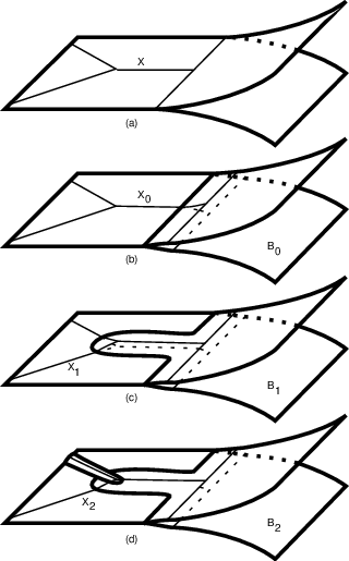
When $n=0$, we begin with $B$ and split in an $\epsilon_{0}$ neighborhood of the branch locus of $B$, see Figure 8ab. This gives a branched surface $B_{0}$ isomorphic to $B$, but now the 1-complex $X$ pulls back, under the projection $\pi_{0}:B_{0}\to B$ to a more complex 1-complex $X_{0}\subset B_{0}$. In particular, the pull-back of some edges of $X$ will be train tracks. We choose a directed 1-cell $\alpha$ of $X_{0}$ emanating from the branch locus of $B_{0}$ and split in an $\epsilon_{1}$ neighborhood of the arc as shown in Figure 8bc. Note that $\alpha$ corresponds to a directed arc in $X$. In fact, $\alpha$ projects to a subarc of a 1-cell in $X$, with at most length $\epsilon$ truncated from each end. It may happen that the final point of $\alpha$ is also on the branch locus of $B_{0}$, so that $\alpha$ is a good directed arc for $B_{0}$. In that case, we must use Lemma 3.1 to decide whether the newly formed branch locus goes over or under the branch locus at the end of the arc. The correct choice ensures that the new branched surface $B_{1}$ which we obtain will have no non-trivial negative tiscs.

We will continue splitting along (pull-backs of) other arcs of $X$, one at a time, to obtain a sequence $B_{n}$ of branched surfaces, each projecting to $B$ via $\pi_{n}:B_{n}\to B$. At the $n$-th step we split on a strip corresponding to an $\epsilon_{n}$ neighborhood of an arc contained in the pull-back train track of a 1-cell of $X$. Note that later splittings are done on thinner strips, older splittings are done on fatter strips as shown in Figure 8. Figure 8cd shows a splitting on a good arc, where Lemma 3.1 is applied to make a choice among possible splittings. At the $n$-th step, we choose to split $B_{n}$ on an arc emanating from the branch locus near a 0-cell, and we do this at the oldest part of the branch locus. This means that we begin the splitting at an available part of the branch locus outermost in a neighborhood of a 0-cell of $X$. This, and the fact that the sequence $\epsilon_{n}$ is decreasing, guarantees that none of the new branch locus “passes” the old branch locus to give a bad move. At the final end of the arc of splitting, however, we may need to apply Lemma 3.1 repeatedly to decide whether the splitting goes over or under the opposing branch locus. The correct choices ensure that $B_{n}$ has no iscs or negative tiscs.

We have projections $p_{n}:B_{n}\to B$. We illustrate a possible sequence of events locally by choosing an edge $e$ in $X$, then examining $p_{n}^{-1}(e)\subset X_{n}$. Figure 9 shows such a sequence of splittings of $e$ induced by the splittings of $B$. The first three splittings are consistent with the splittings induced on the central edge of $X$ in Figure 8.

Denote by $N(X)$ the $\epsilon/2$-neighbourhood of $X$ in $B$. The infinite sequence of splittings as above defines a lamination $\Lambda$ in the preimage $\pi^{-1}(N(X))\subset V(B)$ as an inverse limit of the sequence of projections $q_{n}:B_{j}\to B_{j-1}$

The inverse limit can be realized as a space embedded in $M$, where it is the intersection of appropriately chosen nested neighborhoods $N(B_{j})\hookrightarrow M$. See [4] for more details on constructing laminations as inverse limits.

We can describe the inverse limit in another way. For each splitting in the sequence (including the first splitting from $B$ to $B_{0}$) consider a sheet of surface in $V(B)$ “parallel” to this splitting, i.e. a sheet of surface transverse to the vertical fibers in $V(B)$, with boundary equal to the union of the old and new part of the branch locus corresponding to the splitting. We may think of this sheet as the splitting surface. The union of all such surfaces corresponding to the splittings in the infinite sequence, intersected with the preimage $\pi^{-1}(N(X))$ is a non-compact splitting surface which we call $L$. The lamination $\Lambda$ is obtained from $\pi^{-1}(N(X))\subset V(B)$ by splitting on $L$. Each component of $L$ has boundary, with one arc of the boundary attached to the branch locus $\partial_{v}V(B)$ and the remainder of the boundary in mapped by $\pi$ to the boundary of $N(X)$ in $B$. This follows from the choices of splittings at the oldest parts of branch locus, which guarantees that no part of branch locus in the interior of $\pi^{-1}(N(X))$ remains unaffected by later splittings. Thus we can say that $L$ is carried by $N(X)$.

Crucial for our purposes is the following property of the lamination $\Lambda$ or the splitting surface $L$. Let $E$ be a 2-cell of $B$ and $\hat{E}$ the smaller 2-cell obtained by removing the part of $N(X)$ contained in $E$. Then the intersection with $L$ defines a nonempty immersed 1-dimensional manifold in the annulus $\pi^{-1}(\partial\hat{E})=\partial\hat{E}\times I$ in $V(B)$. The intersection with $\Lambda$ gives a 1-dimensional lamination.

By the construction of $L$ and $\Lambda$, both $L$ and $\Lambda$ have strictly negative holonomy. This means that following any leaf of $L$ or $\Lambda$ in the direction of the orientation induced on $\partial\hat{E}$ from the orientation of $B$, after a full turn around $\hat{E}$, we end at a point in the same vertical fiber lying below the initial point using the canonical orientation of the fibers. (It is an unfortunate fact of life in contact geometry that positive contact structures induce negative holonomy.) To prove this property observe that if it were not true then we would have either a disk of contact (coming from a leaf without holonomy) or a negative twisted disc of contact (coming from a leaf with positive holonomy) for some branched surface $B_{n}$ in our sequence.

We will refer to the above property by saying that the splitting surface $L$ or the lamination $\Lambda$ itself has strictly negative holonomy.

We end this section by noting that the arguments can be extended, without too much difficulty, to the case of a noncompact branched surface $B$.

In this section we start converting the splitting surface $L$ or the lamination $\Lambda$ with strictly negative holonomy into a pure contamination in $V(B)$. As a first step we convert $L$ or $\Lambda$ to a smooth foliation $\cal F$ in $\pi^{-1}(N(X))$.

Without loss of generality we may assume $L$ has the following two further properties:

(1) $L$ is continuous, i.e. the tangent plane $T_{x}L$ depends continuously on the point $x\in L$ (in the topology on $L$ induced from $V(B)$);

(2) for each vertical fiber $I=[a,b]$ in $\pi^{-1}(N(X))$ we have $\sup L\cap I=b$ and $\inf L\cap I=a$.

A continuous foliation $\cal F$ with singular branched leaves with the required properties can also be constructed from the lamination $\Lambda$ roughly as follows. One replaces boundary leaves of $\Lambda$ by product families of leaves, suitably tapered, then one collapses gaps in $V(B)-\Lambda$.

Our next goal is to modify $\cal F$ so that it becomes smooth, and still has strictly negative holonomy.

Using a fiber-preserving homeomorphism of $V(B)$ we can make $\cal F$ smooth near the vertex fibers (i.e. vertical fibers corresponding to vertices of $X$). We can then choose smooth cylindrical charts

in cylinders $E\times I$ with the following properties:

(1) lines $(r,\theta)=\text{constant}$ correspond to vertical fibers of $V(B)$;

(2) for some $\delta>0$, $\pi^{-1}(N_{\epsilon/2}X)\cap E=\{(r,\theta,z):r\geq 1-\delta\}$;

(3) $\cal F$ is given in coordinates $(r,\theta,z)$ as the kernel of a 1-form $dz+f(z,\theta)d\theta$, with $f$ independent of $r$, $f\leq 0$, and $f=0$ only near the arguments $\theta$ corresponding to the vertex fibers in $\partial E\times I$ (where $\cal F$ is smooth).

Consider a 1-cell $A$ of $X$ which is the intersection of two 2-cells $E_{1}$ and $E_{2}$ whose union $E_{1}\cup E_{2}$ is smooth at $A$. We focus on the part of the foliation $\cal F$ restricted to $\pi^{-1}(A)$ (or more precisely, to the intersection of the cylinders in $V(B)$ corresponding to $E_{1}$ and $E_{2}$ in the preimage $\pi^{-1}(A)$). In both charts $(\theta_{1},z_{1})$ and $(\theta_{2},z_{2})$ (in $\partial E_{1}\times I_{1}$ and $\partial E_{2}\times I_{2}$ respectively), this restriction is described by the continuous functions $f_{1}$ and $f_{2}$ as in condition (3) above. We will modify this part of $\cal F$ so that the functions $f_{1}$ and $f_{2}$ become smooth and still satisfy the assertions of condition (3).

Let $f_{1}^{\prime}\geq f_{1}$ be a nonpositive smooth function with the same support as $f_{1}$ (such a function clearly exists). Modify $\cal F$ inside $E_{1}\times I_{1}$ and $E_{2}\times I_{2}$ (only close to $\pi^{-1}(A)$) by making it equal to the kernel of the 1-form $dz_{1}+f_{1}^{\prime}(\theta_{1},z_{1})d\theta_{1}$ and the 1-form $dz_{2}+f_{2}^{\prime}(\theta_{2},z_{2})d\theta_{2}$, where $f_{2}^{\prime}$ is the smooth function induced by $f_{1}^{\prime}$ and the compatibility of modifications at the intersection of the two charts.

The modified foliation still has strictly negative holonomy at $\partial E_{1}\times I_{1}$. The holonomy function is however smaller in absolute value (or at least not bigger) than before modification. Due to the fact that the orientations on $A$ induced by coordinates $\theta_{1}$ and $\theta_{2}$ are opposite, we have $f_{2}^{\prime}\leq f_{2}$, which clearly implies that the holonomy at $\partial E_{2}\times I_{2}$ of the modified foliation is also strictly negative. Since the modification did not affect other cylinders, the holonomy of the modified foliation is strictly negative for all of them. Performing this sort of modification at all edges $A$ in $X$ we get a smooth foliation $\cal F$ as required.

To prove Theorem 1.1 we will further modify the foliation $\cal F$ obtained in the previous section. For this modification, which is presented in Section 7, we need some coordinate charts well suited to the contamination structure. This section contains description of such charts, which are similar to ones used in [6].

Let $\xi$ denote a contamination carried by $B\hookrightarrow M$.

Observe that in view of (3), the image curves in condition (1) coincide with the fibers of $V(B)$.

We mention without proof the following easy fact.

The freedom for constructing $\cal B$-charts for a contamination $\xi$ is similar to that for $\cal C$-charts, see Lemma 6.2. We omit the details.

The advantage of working with $\cal C$-charts and $\cal B$-charts for a contamination $\xi$ carried by $B$ is that in the coordinates provided by these charts $\xi$ can be expressed in a unique way as the kernel of a 1-form $dz+f(r,\theta,z)d\theta$, or $dz+f(x,y,z)dx$, for some smooth function $f$. We will call the function $f$ as above a slope function. It is possible to modify a contamination $\xi$ inside a chart neighbourhood by modifying the appropriate slope function. The following lemmas show how to express the property of being a confoliation (or a contact structure) in terms of a slope function.

The proof of Lemma 6.4 is straightforward, and can be found in [1]. We will include the slightly more difficult proof of Lemma 6.5.

The following lemmas establish the existence of “purifying operations”, which modify a contamination to eliminate portions of the non-contact locus. In particular, we will use these lemmas to remove foliated parts of a contamination obtained (in the next section) from the foliation $\cal F$ by inserting pieces of contact structures in the complement $V(B)\setminus\pi^{-1}(N(X))$.

We wil prove Lemma 6.7 and omit the proof of Lemma 6.6, which is essentially the same.

(1) $f^{\prime}$ coincides with $f$ in the union of the subsets $\{|x|\geq 1-\delta\}$, $\{y\geq y_{1}\}$ and $\{|z|=1\}$ in $\cal B$;

(2) $\partial f^{\prime}/\partial y<0$ in the subset $\{|x|<1-\delta,|z|<1\}$.

To complete the proof of Theorem 1.1 we will further modify the foliation $\cal F$ obtained in Section 5. We will first extend $\cal F$ to an impure contamination $\xi_{0}$ in $V(B)$, by inserting standard pieces of contact structure in the components of $V(B)\setminus\pi^{-1}(N(X))$. Next, we will purify the contamination $\xi_{0}$ using the special charts and purifying operations described in the previous section.

Consider the cell structure in $B$ as in Section 4, with its 1-skeleton $X$ and with 2-cells denoted by $E$. Recall that $\cal F$ is a smooth foliation in $\pi^{-1}(N(X))$ transverse to the fibers in $V(B)$. We can choose in each part $\pi^{-1}(E)$ of $V(B)$ smooth cyllindrical coordinates $(r,\theta,z)$, $|z|\leq 1$, $r\leq R$, with the following properties:

(1) vertical fibers in $\pi^{-1}(E)$ correspond to curves $(r,\theta)=const$;

(2) $\pi^{-1}(E\cap N(X))=\{r\geq r_{0}\}$ for some $0<r_{0}<R$;

(3) $\cal F$ is the kernel of a 1-form $dz+f(\theta,z)d\theta$, where the function $f$ does not depend on $r$.

(4) $f(\theta,z)<0$ for all $|z|<1$ and all $\theta$.

It follows from properties of $f$ that there exists a function $f_{0}$ on $\pi^{-1}(E)$ such that

(a) $f_{0}(r,\theta,z)=f(\theta,z)$ for $r\geq r_{0}$;

(b) $\partial f_{0}/\partial r<0$ at $\{|z|<1,0<r<r_{0}\}$;

(c) $f_{0}=r^{2}\cdot h$ with $h(0,\theta,z)<0$ for all $|z|<1$.

Our goal now is to purify $\xi_{0}$. We do this in the following four steps.

Step 1. Observe that cylindrical charts as above in the parts $\pi^{-1}(E)\subset V(B)$ are in fact $\cal C$-charts for the contamination $\xi_{0}$. Using these $\cal C$-charts and Lemma 6.6(1), we modify $\xi_{0}$ so that, for all $E$, it becomes pure in $\pi^{-1}(E)$. Thus now the locus of interior points of $V(B)$ where $\xi_{0}$ is not contact is contained in the preimage $\pi^{-1}(X)$ of the 1-skeleton $X$.

Step 2. For each edge $e$ in $B$ not in the branch locus one can consider a $\cal B$-chart for $\xi_{0}$ in $V(B)$ so that $e$ corresponds to the curve $y=0$ in $(x,y)$ coordinates of this $\cal B$-chart and so that $\xi_{0}$ is contact at $\{|z|<1,y\neq 0\}\subset{\cal B}$. Using such charts and Lemma 6.7 we can modify $\xi_{0}$ so that the locus of interior points of $V(B)$ where $\xi_{0}$ is not contact is contained in the $\pi$-preimage of an arbitrarily small neighbourhood in $X$ of the branch locus of $B$. Some further purification with use of appropriate $\cal C$-charts and Lemma 6.6(1) makes this locus contained in the preimage of the branch locus of $B$ only.

Step 3. By modifying slope functions in small open $\cal B$-charts adjacent to the circle components in $\partial_{v}V(B)$, we can modify $\xi_{0}$ introducing thin annular leaves adjacent to those circles. This can be done so that the remainder of the locus where $\xi_{0}$ is contact is unchanged. We then split $V(B)$ on the above annular leaves and obtain a neighborhood $V(B^{\prime})$ of an isomorphic branched surface $B^{\prime}$ and the induced contamination $\xi_{0}^{\prime}$ in $V(B^{\prime})$.

Step 4. We can now purify $\xi_{0}^{\prime}$ near the locus where it is not contact inside $V(B^{\prime})$ (we denote this locus by $L$). The locus $L$ is contained in the subset of $V(B^{\prime})$ corresponding (before splitting $B\to B^{\prime}$) to the preimage by $\pi$ of the branch locus of $B$. Denoting by $\pi^{\prime}:V(B^{\prime})\to B^{\prime}$ the natural fiberwise projection in $V(B^{\prime})$, observe that $L$ is disjoint with the preimage by $\pi^{\prime}$ of the branch locus of $B^{\prime}$.

We purify first near the preimage of the regular part of the branch locus in $B$, using Lemma 6.7 in the same manner as in Step 2. Then, we purify near the preimages of the points $P$ in the branch locus of $B$, where two branching lines meet. This can be done using Lemma 6.6 with appropriate $\cal C$-charts. In this way we obtain a pure contamination $\xi$ carried by the branched surface $B^{\prime}$ and, since $B^{\prime}$ is isomorphic to $B$, Theorem 1.1 follows.

References

- [1] Y. M. Eliashberg and W. P. Thurston, Confoliations, University Lecture Series, vol. 13, American Mathematical Society, 1998.
- [2] W. Floyd and U. Oertel, Incompressible surfaces via branched surfaces, Topology 23 (1984), 117–125.
- [3] D. Gabai and U. Oertel, Essential laminations in 3-manifolds, Ann. of Math. 130 (1989), 41–73.
- [4] L. Mosher and U. Oertel, Spaces which are not negatively curved, Comm. in Anal. and Geom. 6 (1991), 67–140.
- [5] U. Oertel, Measured laminations in 3-manifolds, Trans. Am. Math. Soc. 305 (1988), no. 2, 531–573.
- [6] U. Oertel and J. Świa̧tkowski, Contact structures, -confoliations, and contaminations in 3-manifolds, Manuscript, 2001, may soon be posted at http://andromeda.rutgers.edu/ oertel/.
- [7] R. Williams, Expanding attractors, Pub. Math. I.H.E.S. 43 (1974), 169–203.