A geometric realization of spin representations and Young diagrams from quiver varieties

Alistair Savage

Abstract

Applying the techniques of an earlier paper with Frenkel, we develop a geometric realization of spin representations and Clifford algebras. In doing so, we give an explicit parametrization of the irreducible components of Nakajima varieties of type $D$ in terms of Young diagrams. We explicity compute the geometric action of the Lie algebra and are able to extend the geometric action to the entire Clifford algebra used in the classical construction of the spin representations.

^†^†footnotetext: 2000 Mathematics Subject Classification: 17B10 (Primary), 16G20 (Secondary)^†^†footnotetext: Keywords: spin representation, clifford algebra, quiver, geometrization, Young diagram

Introduction

In [FS03], we related two apparently different bases in the representations of affine Lie algebras of type $A$ : one arising from statistical mechanics, the other from gauge theory. In particular, using geometric methods associated to quiver varieties, we were able to give an alternative and much simpler geometric proof of a result of [DJKMO89] on the construction of bases of affine Lie algebra representations. At the same time, we gave a simple parametrization of the irreducible components of Nakajima quiver varieties associated to infinite and cyclic quivers in terms of Young and Maya diagrams. In the current paper, we consider the spin representations of the Lie algebra $\mathfrak{g}=\mathfrak{so}_{2n}\mathbb{C}$ of type $D_{n}$ . Applying the techniques of [FS03], we are able to give a very explicit parametrization of the irreducible components of the associated Nakajima varieties in terms of Young diagrams of strictly decreasing row length with maximum length $n-1$ . We also explicitly compute the geometric action and thus obtain a realization of the spin representations in terms of these diagrams. Furthermore, we are able to extend the geometric action to the entire Clifford algebra used in the classical construction of the spin representations. This is the first example of a geometric realization of additional structure on irreducible representations extending the module structure originally defined by Nakajima. Possible extensions of these results to the affine case may suggest new statistical mechanics results for type $D$ analogous to those of type $A$ mentioned above.

The author would like to thank I. B. Frenkel for numerous discussions and helpful suggestions and M. Kassabov for pointing out an error in an earlier version of this paper. This research was supported in part by the Natural Sciences and Engineering Research Council (NSERC) of Canada and the Clay Mathematics Institute.

1 Lusztig’s Quiver Varieties

In this section, we will recount the explicit description given in [L91] of the irreducible components of Lusztig’s quiver variety for type $D_{n}$ . See this reference for details, including proofs.

1.1 General Definitions

Let $I$ be the set of vertices of the Dynkin graph of a symmetric Kac-Moody Lie algebra $\mathfrak{g}$ and let $H$ be the set of pairs consisting of an edge together with an orientation of it. For $h\in H$ , let $\inc(h)$ (resp. $\out(h)$ ) be the incoming (resp. outgoing) vertex of $h$ . We define the involution $\bar{\ }:H\to H$ to be the function which takes $h\in H$ to the element of $H$ consisting of the same edge with opposite orientation. An orientation of our graph is a choice of a subset $\Omega\subset H$ such that $\Omega\cup\bar{\Omega}=H$ and $\Omega\cap\bar{\Omega}=\emptyset$ .

Let $\mathcal{V}$ be the category of finite-dimensional $I$ -graded vector spaces $\mathbf{V}=\oplus_{i\in I}\mathbf{V}_{i}$ over $\mathbb{C}$ with morphisms being linear maps respecting the grading. Then $\mathbf{V}\in\mathcal{V}$ shall denote that $\mathbf{V}$ is an object of $\mathcal{V}$ . Labelling the vertices of $I$ by $1,\dots,n$ , the dimension of $\mathbf{V}\in\mathcal{V}$ is given by $\mathbf{v}=\dim\mathbf{V}=(\dim\mathbf{V}_{1},\dots,\dim\mathbf{V}_{n})$ .

Given $\mathbf{V}\in\mathcal{V}$ , let

\mathbf{E_{V}}=\bigoplus_{h\in H}\Hom(\mathbf{V}_{\out(h)},\mathbf{V}_{\inc(h)}).

For any subset $H^{\prime}$ of $H$ , let $\mathbf{E}_{\mathbf{V},H^{\prime}}$ be the subspace of $\mathbf{E_{V}}$ consisting of all vectors $x=(x_{h})$ such that $x_{h}=0$ whenever $h\not\in H^{\prime}$ . The algebraic group $G_{\mathbf{V}}=\prod_{i}\Aut(\mathbf{V}_{i})$ acts on $\mathbf{E_{V}}$ and $\mathbf{E}_{\mathbf{V},H^{\prime}}$ by

(g,x)=((g_{i}),(x_{h}))\mapsto gx=(x^{\prime}_{h})=(g_{\inc(h)}x_{h}g_{\out(h)}^{-1}).

Define the function $\varepsilon:H\to\{-1,1\}$ by $\varepsilon(h)=1$ for all $h\in\Omega$ and $\varepsilon(h)=-1$ for all $h\in{\bar{\Omega}}$ . For $\mathbf{V}\in\mathcal{V}$ , the Lie algebra of $G_{\mathbf{V}}$ is $\mathbf{gl_{V}}=\prod_{i}\End(\mathbf{V}_{i})$ and it acts on $\mathbf{E_{V}}$ by

(a,x)=((a_{i}),(x_{h}))\mapsto[a,x]=(x^{\prime}_{h})=(a_{\inc(h)}x_{h}-x_{h}a_{\out(h)}).

Let $\left<\cdot,\cdot\right>$ be the nondegenerate, $G_{\mathbf{V}}$ -invariant, symplectic form on $\mathbf{E_{V}}$ with values in $\mathbb{C}$ defined by

\left<x,y\right>=\sum_{h\in H}\varepsilon(h)\tr(x_{h}y_{\bar{h}}).

Note that $\mathbf{E_{V}}$ can be considered as the cotangent space of $\mathbf{E}_{\mathbf{V},\Omega}$ under this form.

The moment map associated to the $G_{\mathbf{V}}$ -action on the symplectic vector space $\mathbf{E_{V}}$ is the map $\psi:\mathbf{E_{V}}\to\mathbf{gl_{V}}$ with $i$ -component $\psi_{i}:\mathbf{E_{V}}\to\End\mathbf{V}_{i}$ given by

\psi_{i}(x)=\sum_{h\in H,\,\inc(h)=i}\varepsilon(h)x_{h}x_{\bar{h}}.

Definition 1.1 ([L91]).

An element $x\in\mathbf{E_{V}}$ is said to be nilpotent if there exists an $N\geq 1$ such that for any sequence $h^{\prime}_{1},h^{\prime}_{2},\dots,h^{\prime}_{N}$ in $H$ satisfying $\out(h^{\prime}_{1})=\inc(h^{\prime}_{2})$ , $\out(h^{\prime}_{2})=\inc(h^{\prime}_{3})$ , …, $\out(h^{\prime}_{N-1})=\inc(h^{\prime}_{N})$ , the composition $x_{h^{\prime}_{1}}x_{h^{\prime}_{2}}\dots x_{h^{\prime}_{N}}:\mathbf{V}_{\out(h^{\prime}_{N})}\to\mathbf{V}_{\inc(h^{\prime}_{1})}$ is zero.

Definition 1.2 ([L91]).

Let $\Lambda_{\mathbf{V}}$ be the set of all nilpotent elements $x\in\mathbf{E_{V}}$ such that $\psi_{i}(x)=0$ for all $i\in I$ .

1.2 Type $D_{n}$

Let $\mathfrak{g}=\mathfrak{so}_{2n}\mathbb{C}$ be the simple Lie algebra of type $D_{n}$ . Let $I=\{1,2,\dots,n\}$ be the set of vertices of the Dynkin graph of $\mathfrak{g}$ , labelled as in Figure 1.

Refer to caption — Figure 1: The Dynkin graph of type $D_{n}$ . We represent the $n$ th vertex by an open dot to distinguish it from the $(n-1)$ st vertex.

We let $\Omega$ be the orientation indicated in Figure 2.

Label each oriented edge by its incoming and outgoing vertices. That is, if vertices $i$ and $j$ are connected by an edge, $h_{i,j}$ denotes the oriented edge with $\out(h)=i$ , $\inc(h)=j$ . The following is proven in [L91, Proposition 14.2].

Proposition 1.3.

The irreducible components of $\Lambda_{\mathbf{V}}$ are the closures of the conormal bundles of the various $G_{\mathbf{V}}$ -orbits in $\mathbf{E}_{\mathbf{V},\Omega}$ .

For two integers $1\leq k^{\prime}\leq k\leq n-1$ , define $\mathbf{V}(k^{\prime},k)\in\mathcal{V}$ to be the vector space with basis $\{e_{r}\ |\ k^{\prime}\leq r\leq k\}$ . We require that $e_{r}$ has degree $r\in I$ . Let $x(k^{\prime},k)\in\mathbf{E}_{\mathbf{V}(k^{\prime},k),\Omega}$ be defined by $x(k^{\prime},k)_{h_{r,r+1}}:e_{r}\mapsto e_{r+1}$ for $k^{\prime}\leq r<k$ , and all other components of $x(k^{\prime},k)$ are zero. We picture this representation as the string of Figure 3.

For an integer $k^{\prime}$ such that $1\leq k^{\prime}\leq n-2$ or $k^{\prime}=n$ , define $\mathbf{V}(k^{\prime},n)$ to be the vector space with basis $\{e_{r}\ |\ k^{\prime}\leq r\leq n-2\text{ or }r=n\}$ . Again, we require that $e_{r}$ has degree $r\in I$ . Let $x(k^{\prime},n)\in\mathbf{E}_{\mathbf{V}(k^{\prime},n),\Omega}$ be defined by

	$\displaystyle x(k^{\prime},n)_{h_{r,r+1}}(e_{r})$	$\displaystyle=\begin{cases}e_{r+1}&\text{if $r<n-2$}\\ 0&\text{otherwise}\end{cases},$
	$\displaystyle x(k^{\prime},n)_{h_{n-2,n}}(e_{n-2})$	$\displaystyle=e_{n}$

and all other components of $x(k^{\prime},k)$ are zero. We picture this representation as the string of Figure 4.

Next, for an integer $k^{\prime}$ such that $1\leq k^{\prime}\leq n-2$ , define $\mathbf{V}(k^{\prime},n+1)$ to be the vector space with basis $\{e_{r}\ |\ k^{\prime}\leq r\leq n\}$ where the degree of $e_{r}$ is $r\in I$ . $x(k^{\prime},n+1)$ is defined by

	$\displaystyle x(k^{\prime},n+1)_{h_{r,r+1}}(e_{r})$	$\displaystyle=\begin{cases}e_{r+1}&\text{if $r\leq n-2$}\\ 0&\text{otherwise}\end{cases},$
	$\displaystyle x(k^{\prime},n+1)_{h_{n-2,n}}(e_{n-2})$	$\displaystyle=e_{n}$

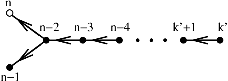
and all other components of $x(k^{\prime},n+1)$ are zero. We picture this representation as the (forked) string of Figure 5.

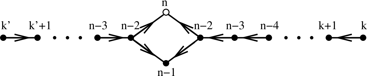
Finally, for $1\leq k^{\prime}<k\leq n-2$ , let ${\widetilde{\mathbf{V}}}(k^{\prime},k)$ be the vector space with basis $\{e_{r}\,|\,k\leq r\leq n\}\cup\{{\tilde{e}}_{r}\,|\,k^{\prime}\leq r\leq n-2\}$ where the degree of $e_{r}$ and ${\tilde{e}}_{r}$ is $r\in I$ . Let ${\tilde{x}}(k^{\prime},k)$ be defined by

	$\displaystyle{\tilde{x}}(k^{\prime},k)_{h_{r,r+1}}(e_{r})$	$\displaystyle=\begin{cases}e_{r+1}&\text{if $r\geq n-2$},\\ 0&\text{otherwise}\end{cases},$
	$\displaystyle{\tilde{x}}(k^{\prime},k)_{h_{r,r+1}}({\tilde{e}}_{r})$	$\displaystyle=\begin{cases}{\tilde{e}}_{r+1}&\text{if $r<n-2$},\\ e_{n-1}&\text{if $r=n-2$}\\ 0&\text{otherwise}\end{cases},$
	$\displaystyle{\tilde{x}}(k^{\prime},k)_{h_{n-2,n}}(e_{n-2})$	$\displaystyle=e_{n}$
	$\displaystyle{\tilde{x}}(k^{\prime},k)_{h_{n-2,n}}({\tilde{e}}_{n-2})$	$\displaystyle=e_{n}$

and all other components of ${\tilde{x}}(k^{\prime},k)$ are zero. We picture this representation as the string of Figure 6.

Proposition 1.4.

The above $(\mathbf{V}(k^{\prime},k),x(k^{\prime},k))$ and $({\widetilde{\mathbf{V}}}(k^{\prime},k),{\tilde{x}}(k^{\prime},k))$ are indecomposable representations of the $D_{n}$ quiver with orientation $\Omega$ . Conversely, any indecomposable finite-dimensional representation $(\mathbf{V},x)$ of this quiver is isomorphic to one of these representations.

Proof.

It is easy to see that each of the above representations is indecomposable. The fact that our list is exhaustive follows from the fact that the indecomposable representations of the $D_{n}$ quiver are in one-to-one correspondence with the positive roots of the Lie algebra of type $D_{n}$ (see [K80, K83]). $\hfill\square$

Let

	$\displaystyle Z=$	$\displaystyle\{(k^{\prime},k)\,\|\,(k^{\prime},k)\neq(n-1,n),(n-1,n+1),(n,n+1),(n+1,n+1)\}$
		$\displaystyle\cup\{(k^{\prime},k)^{\sim}\,\|\,1\leq k^{\prime}<k\leq n-2\},$

and let $\tilde{Z}$ be the set of all functions $Z\to\mathbb{Z}_{\geq 0}$ with finite support. It is clear that for $\mathbf{V}\in\mathcal{V}$ , the set of $G_{\mathbf{V}}$ -orbits in $\mathbf{E}_{\mathbf{V},\Omega}$ is naturally indexed by the subset $\tilde{Z}_{\mathbf{V}}$ of $\tilde{Z}$ consisting of those $f\in\tilde{Z}$ such that

\sum_{A(k^{\prime},k)\ni i}f(k^{\prime},k)+\sum_{B(k^{\prime},k)\ni i}f((k^{\prime},k)^{\sim})(\dim{\widetilde{\mathbf{V}}}(k^{\prime},k))_{i}=\dim\mathbf{V}_{i}\hskip 10.00002pt\forall\ i\in I

where $A(k^{\prime},k)$ is the set of all $i\in I$ such that $\mathbf{V}(k^{\prime},k)$ contains a vector of degree $i$ and $B(k^{\prime},k)$ is the set of all $i\in I$ such that ${\widetilde{\mathbf{V}}}(k^{\prime},k)$ contains a vector of degree $i$ . Note that we write $f(k^{\prime},k)$ for $f((k^{\prime},k))$ . Corresponding to a given $f$ is the orbit consisting of all representations isomorphic to a sum of the indecomposable representations $x(k^{\prime},k)$ and ${\tilde{x}}(k^{\prime},k)$ , each occurring with multiplicity $f(k^{\prime},k)$ and $f((k^{\prime},k)^{\sim})$ respectively. Denote by $\mathcal{O}_{f}$ the $G_{\mathbf{V}}$ -orbit corresponding to $f\in\tilde{Z}_{\mathbf{V}}$ . Let $\mathcal{C}_{f}$ be the conormal bundle to $\mathcal{O}_{f}$ and let $\bar{\mathcal{C}}_{f}$ be its closure. We then have the following proposition.

Proposition 1.5.

The map $f\to\bar{\mathcal{C}}_{f}$ is a one-to-one correspondence between the set $\tilde{Z}_{\mathbf{V}}$ and the set of irreducible components of $\Lambda_{\mathbf{V}}$ .

Proof.

This follows immediately from Propositions 1.3 and 1.4. $\hfill\square$

2 Nakajima’s Quiver Varieties

We introduce here a description of the quiver varieties first presented in [N94] for type $D_{n}$ .

Definition 2.1 ([N94]).

For $\mathbf{v},\mathbf{w}\in\mathbb{Z}_{\geq 0}^{I}$ , choose $I$ -graded vector spaces $\mathbf{V}$ and $\mathbf{W}$ of graded dimensions $\mathbf{v}$ and $\mathbf{w}$ respectively. Then define

\Lambda\equiv\Lambda(\mathbf{v},\mathbf{w})=\Lambda_{\mathbf{V}}\times\sum_{i\in I}\Hom(\mathbf{V}_{i},\mathbf{W}_{i}).

Now, suppose that $\mathbf{S}$ is an $I$ -graded subspace of $\mathbf{V}$ . For $x\in\Lambda_{\mathbf{V}}$ we say that $\mathbf{S}$ is $x$ -stable if $x(\mathbf{S})\subset\mathbf{S}$ .

Definition 2.2 ([N94]).

Let $\Lambda^{\text{st}}=\Lambda(\mathbf{v},\mathbf{w})^{\text{st}}$ be the set of all $(x,j)\in\Lambda(\mathbf{v},\mathbf{w})$ satisfying the following condition: If $\mathbf{S}=(\mathbf{S}_{i})$ with $\mathbf{S}_{i}\subset\mathbf{V}_{i}$ is $x$ -stable and $j_{i}(\mathbf{S}_{i})=0$ for $i\in I$ , then $\mathbf{S}_{i}=0$ for $i\in I$ .

The group $G_{\mathbf{V}}$ acts on $\Lambda(\mathbf{v},\mathbf{w})$ via

(g,(x,j))=((g_{i}),((x_{h}),(j_{i})))\mapsto((g_{\inc(h)}x_{h}g_{\out(h)}^{-1}),(j_{i}g_{i}^{-1})).

and the stabilizer of any point of $\Lambda(\mathbf{v},\mathbf{w})^{\text{st}}$ in $G_{\mathbf{V}}$ is trivial (see [N98, Lemma 3.10]). We then make the following definition.

Definition 2.3 ([N94]).

Let $\mathcal{L}\equiv\mathcal{L}(\mathbf{v},\mathbf{w})=\Lambda(\mathbf{v},\mathbf{w})^{\text{st}}/G_{\mathbf{V}}$ .

Let $\Irr\mathcal{L}(\mathbf{v},\mathbf{w})$ (resp. $\Irr\Lambda(\mathbf{v},\mathbf{w})$ ) be the set of irreducible components of $\mathcal{L}(\mathbf{v},\mathbf{w})$ (resp. $\Lambda(\mathbf{v},\mathbf{w})$ ). Then $\Irr\mathcal{L}(\mathbf{v},\mathbf{w})$ can be identified with

\{Y\in\Irr\Lambda(\mathbf{v},\mathbf{w})\,|\,Y\cap\Lambda(\mathbf{v},\mathbf{w})^{\text{st}}\neq\emptyset\}.

Specifically, the irreducible components of $\Irr\mathcal{L}(\mathbf{v},\mathbf{w})$ are precisely those

X_{f}\stackrel{{\scriptstyle\text{def}}}{{=}}\left(\left(\bar{\mathcal{C}}_{f}\times\sum_{i\in I}\Hom(\mathbf{V}_{i},\mathbf{W}_{i})\right)\cap\Lambda(\mathbf{v},\mathbf{w})^{\text{st}}\right)/G_{\mathbf{V}}

which are nonempty.

The following will be used in the sequel.

Lemma 2.4.

One has

\Lambda^{\text{st}}=\left\{x\in\Lambda\,\left|\,\ker j_{i}\cap\bigcap_{h:\out(h)=i}\ker x_{h}=0\ \forall\ i\right.\right\}.

Proof.

Since each $\bigcap_{h:\out{h}=i}\ker x_{h}$ is $x$ -stable, the left hand side is obviously contained in the right hand side. Now suppose $x$ is an element of the right hand side. Let $\mathbf{S}=(\mathbf{S}_{i})$ with $\mathbf{S}_{i}\subset\mathbf{V}_{i}$ be $x$ -stable and $j_{i}(\mathbf{S}_{i})=0$ for $i\in I$ . Assume that $\mathbf{S}\neq 0$ . Since all elements of $\Lambda$ are nilpotent, we can find a minimal value of $N$ such that the condition in Definition 1.1 is satisfied. Then we can find a $v\in\mathbf{S}_{i}$ for some $i$ and a sequence $h_{1}^{\prime},h_{2}^{\prime},\dots,h_{N-1}^{\prime}$ (empty if $N=1$ ) in $H$ such that $\out(h_{1}^{\prime})=\inc(h_{2}^{\prime})$ , $\out(h_{2}^{\prime})=\inc(h_{3}^{\prime})$ , …, $\out(h_{N-2}^{\prime})=\inc(h_{N-1}^{\prime})$ and $v^{\prime}=x_{h_{1}^{\prime}}x_{h_{2}^{\prime}}\dots x_{h_{N-1}^{\prime}}(v)\neq 0$ . Now, $v^{\prime}\in\mathbf{S}_{i^{\prime}}$ for some $i^{\prime}\in I$ by the stability of $\mathbf{S}$ (hence $j_{i^{\prime}}(v^{\prime})=0$ ) and $v^{\prime}\in\bigcap_{h:\out{h}=i^{\prime}}\ker x_{h}$ by our choice of $N$ . This contradicts the fact that $x$ is an element of the right hand side. $\hfill\square$

3 The Lie Algebra Action

We summarize here some results from [N94] that will be needed in the sequel. See this reference for more details, including proofs. We keep the notation of Sections 1 and 2.

Let $\mathbf{w,v,v^{\prime},v^{\prime\prime}}\in\mathbb{Z}_{\geq 0}^{I}$ be such that $\mathbf{v}=\mathbf{v^{\prime}}+\mathbf{v^{\prime\prime}}$ . Consider the maps

\Lambda(\mathbf{v}^{\prime\prime},\mathbf{0})\times\Lambda(\mathbf{v}^{\prime},\mathbf{w})\stackrel{{\scriptstyle p_{1}}}{{\leftarrow}}\mathbf{\tilde{F}(v,w;v^{\prime\prime})}\stackrel{{\scriptstyle p_{2}}}{{\rightarrow}}\mathbf{F(v,w;v^{\prime\prime})}\stackrel{{\scriptstyle p_{3}}}{{\rightarrow}}\Lambda(\mathbf{v},\mathbf{w}),

(3.1)

where the notation is as follows. A point of $\mathbf{F(v,w;v^{\prime\prime})}$ is a point $(x,j)\in\Lambda(\mathbf{v},\mathbf{w})$ together with an $I$ -graded, $x$ -stable subspace $\mathbf{S}$ of $\mathbf{V}$ such that $\dim\mathbf{S}=\mathbf{v^{\prime}}=\mathbf{v}-\mathbf{v^{\prime\prime}}$ . A point of $\mathbf{\tilde{F}(v,w;v^{\prime\prime})}$ is a point $(x,j,\mathbf{S})$ of $\mathbf{F(v,w;v^{\prime\prime})}$ together with a collection of isomorphisms $R^{\prime}_{i}:\mathbf{V}^{\prime}_{i}\cong\mathbf{S}_{i}$ and $R^{\prime\prime}_{i}:\mathbf{V}^{\prime\prime}_{i}\cong\mathbf{V}_{i}/\mathbf{S}_{i}$ for each $i\in I$ . Then we define $p_{2}(x,j,\mathbf{S},R^{\prime},R^{\prime\prime})=(x,j,\mathbf{S})$ , $p_{3}(x,j,\mathbf{S})=(x,j)$ and $p_{1}(x,j,\mathbf{S},R^{\prime},R^{\prime\prime})=(x^{\prime\prime},x^{\prime},j^{\prime})$ where $x^{\prime\prime},x^{\prime},j^{\prime}$ are determined by

	$\displaystyle R^{\prime}_{\inc(h)}x^{\prime}_{h}$	$\displaystyle=x_{h}R^{\prime}_{\out(h)}:\mathbf{V}^{\prime}_{\out(h)}\to\mathbf{S}_{\inc(h)},$
	$\displaystyle j^{\prime}_{i}$	$\displaystyle=j_{i}R^{\prime}_{i}:\mathbf{V}^{\prime}_{i}\to\mathbf{W}_{i}$
	$\displaystyle R^{\prime\prime}_{\inc(h)}x^{\prime\prime}_{h}$	$\displaystyle=x_{h}R^{\prime\prime}_{\out(h)}:\mathbf{V}^{\prime\prime}_{\out(h)}\to\mathbf{V}_{\inc(h)}/\mathbf{S}_{\inc(h)}.$

It follows that $x^{\prime}$ and $x^{\prime\prime}$ are nilpotent.

Lemma 3.1 ([N94, Lemma 10.3]).

One has

(p_{3}\circ p_{2})^{-1}(\Lambda(\mathbf{v},\mathbf{w})^{\text{st}})\subset p_{1}^{-1}(\Lambda(\mathbf{v}^{\prime\prime},\mathbf{0})\times\Lambda(\mathbf{v}^{\prime},\mathbf{w})^{\text{st}}).

Thus, we can restrict (3.1) to $\Lambda^{\text{st}}$ , forget the $\Lambda(\mathbf{v}^{\prime\prime},\mathbf{0})$ -factor and consider the quotient by $G_{\mathbf{V}}$ , $G_{\mathbf{V^{\prime}}}$ . This yields the diagram

\mathcal{L}(\mathbf{v^{\prime}},\mathbf{w})\stackrel{{\scriptstyle\pi_{1}}}{{\leftarrow}}\mathcal{F}(\mathbf{v},\mathbf{w};\mathbf{v}-\mathbf{v^{\prime}})\stackrel{{\scriptstyle\pi_{2}}}{{\rightarrow}}\mathcal{L}(\mathbf{v},\mathbf{w}),

(3.2)

where

\mathcal{F}(\mathbf{v},\mathbf{w},\mathbf{v}-\mathbf{v^{\prime}})\stackrel{{\scriptstyle\text{def}}}{{=}}\{(x,j,\mathbf{S})\in\mathbf{F(v,w;v-v^{\prime})}\,|\,(x,j)\in\Lambda(\mathbf{v},\mathbf{w})^{\text{st}}\}/G_{\mathbf{V}}.

Let $M(\mathcal{L}(\mathbf{v},\mathbf{w}))$ be the vector space of all constructible functions on $\mathcal{L}(\mathbf{v},\mathbf{w})$ . For a subvariety $Y$ of a variety $A$ , let $\mathbf{1}_{Y}$ denote the function on $A$ which takes the value 1 on $Y$ and 0 elsewhere. Let $\chi(Y)$ denote the Euler characteristic of the algebraic variety $Y$ . Then for a map $\pi$ between algebraic varieties $A$ and $B$ , let $\pi_{!}$ denote the map between the abelian groups of constructible functions on $A$ and $B$ given by

\pi_{!}(\mathbf{1}_{Y})(y)=\chi(\pi^{-1}(y)\cap Y),\ Y\subset A

and let $\pi^{*}$ be the pullback map from functions on $B$ to functions on $A$ acting as $\pi^{*}f(y)=f(\pi(y))$ . Then define

		$\displaystyle H_{i}:M(\mathcal{L}(\mathbf{v},\mathbf{w}))\to M(\mathcal{L}(\mathbf{v},\mathbf{w}));\hskip 10.00002ptH_{i}f=u_{i}f,$
		$\displaystyle E_{i}:M(\mathcal{L}(\mathbf{v},\mathbf{w}))\to M(\mathcal{L}(\mathbf{v}-\mathbf{e}^{i},\mathbf{w}));\hskip 10.00002ptE_{i}f=(\pi_{1})_{!}(\pi_{2}^{*}f),$
		$\displaystyle F_{i}:M(\mathcal{L}(\mathbf{v}-\mathbf{e}^{i},\mathbf{w}))\to M(\mathcal{L}(\mathbf{v},\mathbf{w}));\hskip 10.00002ptF_{i}g=(\pi_{2})_{!}(\pi_{1}^{*}g).$

Here

\mathbf{u}={{}^{t}(u_{0},\dots,u_{n})}=\mathbf{w}-C\mathbf{v}

where $C$ is the Cartan matrix of $\mathfrak{g}$ and we are using diagram (3.2) with $\mathbf{v}^{\prime}=\mathbf{v}-\mathbf{e}^{i}$ where $\mathbf{e}^{i}$ is the vector whose components are given by $\mathbf{e}^{i}_{j}=\delta_{ij}$ .

Now let $\varphi$ be the constant function on $\mathcal{L}(\mathbf{0},\mathbf{w})$ with value 1. Let $L(\mathbf{w})$ be the vector space of functions generated by acting on $\varphi$ with all possible combinations of the operators $F_{i}$ . Then let $L(\mathbf{v},\mathbf{w})=M(\mathcal{L}(\mathbf{v},\mathbf{w}))\cap L(\mathbf{w})$ .

Proposition 3.2 ([N94, Thm 10.14]).

The operators $E_{i}$ , $F_{i}$ , $H_{i}$ on $L(\mathbf{w})$ provide the structure of the irreducible highest weight integrable representation of $\mathfrak{g}$ with highest weight $\mathbf{w}$ . Each summand of the decomposition $L(\mathbf{w})=\bigoplus_{\mathbf{v}}L(\mathbf{v},\mathbf{w})$ is a weight space with weight $\mathbf{w}-C\mathbf{v}$ . That is, with weight

\sum_{i\in I}(\mathbf{w}-C\mathbf{v})_{i}\Lambda_{i}

where the $\Lambda_{i}$ are the fundamental weights of $\mathfrak{g}$ (i.e. $\Lambda_{i}(\alpha_{j})=\delta_{ij}$ where $\alpha_{j}$ is the simple root corresponding to the vertex $j$ ).

Let $X\in\Irr\mathcal{L}(\mathbf{v},\mathbf{w})$ and define a linear map $T_{X}:L(\mathbf{v},\mathbf{w})\to\mathbb{C}$ as in [L92, 3.8]. The map $T_{X}$ associates to a constructible function $f\in L(\mathbf{v},\mathbf{w})$ the (constant) value of $f$ on a suitable open dense subset of $X$ . The fact that $L(\mathbf{v},\mathbf{w})$ is finite-dimensional allows us to take such an open set on which any $f\in L(\mathbf{v},\mathbf{w})$ is constant. So we have a linear map

\Phi:L(\mathbf{v},\mathbf{w})\to\mathbb{C}^{\Irr\mathcal{L}(\mathbf{v},\mathbf{w})}.

The following proposition is proved in [L92, 4.16] (slightly generalized in [N94, Proposition 10.15]).

Proposition 3.3.

The map $\Phi$ is an isomorphism; for any $X\in\Irr\mathcal{L}(\mathbf{v},\mathbf{w})$ , there is a unique function $g_{X}\in L(\mathbf{v},\mathbf{w})$ such that for some open dense subset $O$ of $X$ we have $g_{X}|_{O}=1$ and for some closed $G_{\mathbf{V}}$ -invariant subset $K\subset\mathcal{L}(\mathbf{v},\mathbf{w})$ of dimension $<\dim\mathcal{L}(\mathbf{v},\mathbf{w})$ we have $g_{X}=0$ outside $X\cup K$ . The functions $g_{X}$ for $X\in\Irr\Lambda(\mathbf{v},\mathbf{w})$ form a basis of $L(\mathbf{v},\mathbf{w})$ .

4 Geometric Realization of the Spin Representations

We now seek to describe the irreducible components of Nakajima’s quiver variety corresponding to the spin representations of the Lie algebra $\mathfrak{g}$ of type $D_{n}$ . By the comment made in Section 2, it suffices to determine which irreducible components of $\Lambda(\mathbf{v},\mathbf{w})$ are not killed by the stability condition. By Definition 2.1 and Lemma 2.4, these are precisely those irreducible components which contain points $x$ such that

\dim\left(\bigcap_{h:\out(h)=i}\ker x_{h}\right)\leq\mathbf{w}_{i}\ \forall\ i.

(4.1)

We will consider the spin representations of highest weights $\Lambda_{n-1}$ and $\Lambda_{n}$ which correspond to $\mathbf{w}=\mathbf{w}^{n-1}$ and $\mathbf{w}^{n}$ respectively, where $\mathbf{w}^{i}_{j}=\delta_{ij}$ .

Let $\mathcal{Y}$ be the set of all Young diagrams with strictly decreasing row lengths of length at most $n-1$ , that is, the set of all strictly decreasing sequences $(l_{1},\dots,l_{s})$ of non-negative integers ( $l_{j}=0$ for $j>s$ ) such that $l_{1}\leq n-1$ . We will use the terms Young diagram and partition interchangeably. For $Y=(l_{1},\dots,l_{s})\in\mathcal{Y}$ and $1\leq i\leq s$ , let

	$\displaystyle A_{l_{i}}^{+}$	$\displaystyle=\begin{cases}(n-l_{i},n)&\text{if $i$ is odd and $l_{i}>1$}\\ (n,n)&\text{if $i$ is odd and $l_{i}=1$}\\ (n-l_{i},n-1)&\text{if $i$ is even}\end{cases},$
	$\displaystyle A_{l_{i}}^{-}$	$\displaystyle=\begin{cases}(n-l_{i},n)&\text{if $i$ is even and $l_{i}>1$}\\ (n,n)&\text{if $i$ is even and $l_{i}=1$}\\ (n-l_{i},n-1)&\text{if $i$ is odd}\end{cases}$

and let

A_{Y}^{\pm}=\bigcup_{i=1}^{s}A_{l_{i}}^{\pm}.

Theorem 4.1.

The irreducible components of $\mathcal{L}(\mathbf{v},\mathbf{w}^{n})$ (resp. $\mathcal{L}(\mathbf{v},\mathbf{w}^{n-1})$ ) are precisely those $X_{f}$ where $f\in\tilde{Z}_{\mathbf{V}}$ such that

\{(k^{\prime},k)\ |\ f(k^{\prime},k)=1\}=A_{Y}^{\pm}

for some $Y\in\mathcal{Y}$ , $f(k^{\prime},k)=0$ for $(k^{\prime},k)\not\in A_{Y}^{\pm}$ , and $f((k^{\prime},k)^{\sim})=0$ for all $(k^{\prime},k)$ . Denote the component corresponding to such an $f$ by $X_{Y}^{\pm}$ . Thus, $Y\leftrightarrow X_{Y}^{\pm}$ is a natural 1-1 correspondence between the set $\mathcal{Y}$ and the irreducible components of $\cup_{\mathbf{v}}\mathcal{L}(\mathbf{v},\mathbf{w}^{n})$ (resp. $\cup_{\mathbf{v}}\mathcal{L}(\mathbf{v},\mathbf{w}^{n-1})$ ). Here the plus signs correspond to the case $\cup_{\mathbf{v}}\mathcal{L}(\mathbf{v},\mathbf{w}^{n})$ and the minus signs correspond to the case $\cup_{\mathbf{v}}\mathcal{L}(\mathbf{v},\mathbf{w}^{n-1})$ .

Proof.

We prove only the $\cup_{\mathbf{v}}\mathcal{L}(\mathbf{v},\mathbf{w}^{n})$ case. The other case in analogous. Consider the two representations $(\mathbf{V}(k_{1}^{\prime},k_{1}),x(k_{1}^{\prime},k_{1}))$ and $(\mathbf{V}(k_{2}^{\prime},k_{2}),x(k_{2}^{\prime},k_{2}))$ , $1\leq k^{\prime}\leq k\leq n-1$ of our oriented graph as described in Section 1 where the basis of $\mathbf{V}(k_{i}^{\prime},k_{i})$ is $\{e^{i}_{r}\ |\ k_{i}^{\prime}\leq r\leq k_{i}\}$ . Let $W$ be the conormal bundle to the $G_{\mathbf{V}}$ -orbit through the point

x_{\Omega}=(x_{h})_{h\in\Omega}=x(k_{1}^{\prime},k_{1})\oplus x(k_{2}^{\prime},k_{2})\in\mathbf{E}_{\mathbf{V}(k_{1}^{\prime},k_{1})\oplus\mathbf{V}(k_{2}^{\prime},k_{2}),\Omega}.

By the proof of Theorem 5.1 of [FS03], we see that for

x=(x_{\Omega},x_{\bar{\Omega}})=((x_{h})_{h\in\Omega},(x_{h})_{h\in{\bar{\Omega}}})=(x_{h})_{h\in H}\in W,

all of $V(k_{2}^{\prime},k_{2})$ must be in the kernel of $x_{\bar{\Omega}}$ unless $k_{2}^{\prime}>k_{1}^{\prime}$ and $k_{2}>k_{1}$ . If these conditions are satisfied, there exists a point $(x_{\Omega},x_{\bar{\Omega}})\in W$ such that $x_{h_{i,i-1}}(e^{2}_{i})=ce^{1}_{i-1}$ for all $k_{1}+1\leq i\leq k_{2}^{\prime}$ (for a fixed non-zero $c$ ). We picture such a representation as in Figure 7.

Similarly, for the two represenations $(\mathbf{V}(k_{1}^{\prime},n),x(k_{1}^{\prime},n))$ and $(\mathbf{V}(k_{2}^{\prime},n),x(k_{2}^{\prime},n))$ , Both $\mathbf{V}(k_{1}^{\prime},n)$ and $\mathbf{V}(k_{2}^{\prime},n)$ are in the kernel of any component $x_{h}$ , $h\in{\bar{\Omega}}$ of a point in the conormal bundle to the orbit through $x(k_{1}^{\prime},n)\oplus x(k_{2}^{\prime},n)$ (since the left endpoints of the strings are the same).

However, for $k_{1}^{\prime}<k_{2}^{\prime}$ , there are points $x$ in the conormal bundle to the orbit through $x(k_{1}^{\prime},n)\oplus x(k_{2}^{\prime},n-1)$ such that $x_{h_{i,i-1}}(e^{2}_{i})=ce^{1}_{i-1}$ for all $k_{2}^{\prime}\leq i\leq n-1$ and some non-zero $c$ . These maps do not violate the moment map condition since the left endpoints of the two strings are different. Such a representation is pictured as in Figure 8. By symmetry, reversing the roles of $n-1$ and $n$ , there are points $x$ in the conormal bundle to the orbit through $x(k_{1}^{\prime},n-1)\oplus x(k_{2}^{\prime},n)$ such that $x_{h_{n,n-2}}(e^{2}_{n})=ce^{1}_{n-2}$ and $x_{h_{i,i-1}}(e^{2}_{i})=ce^{1}_{i-1}$ for all $k_{2}^{\prime}\leq i\leq n-2$ and some non-zero $c$ if and only if $k_{1}^{\prime}<k_{2}^{\prime}$

Now consider the representations $(\mathbf{V}(k_{1}^{\prime},n-1),x(k_{1}^{\prime},n-1))$ and $(\mathbf{V}(k_{2}^{\prime},n+1),x(k_{2}^{\prime},n+1))$ . Suppose there exists a point $(x_{\Omega},x_{\bar{\Omega}})$ in the conormal bundle to the orbit through the point $x(k_{1}^{\prime},n-1)\oplus x(k_{2}^{\prime},n+1)$ such that $(\mathbf{V}(k_{2}^{\prime},n+1),x(k_{2}^{\prime},n+1))$ is not contained in the kernel of $x_{\bar{\Omega}}$ . Then there is some basis element $e^{2}_{i}\in\mathbf{V}(k_{2}^{\prime},n+1)$ that is not killed by $x_{\bar{\Omega}}$ . This implies that $x_{h_{i,i-1}}(e^{2}_{i})=ce^{1}_{i-1}$ for some $c\neq 0$ since $x_{h_{i,i-1}}(e^{2}_{i})$ can have no $e^{2}_{i-1}$ component by nilpotency. As the cases above, this implies $k_{2}^{\prime}>k_{1}^{\prime}$ .

Now, let $x=(x_{\Omega},x_{\bar{\Omega}})$ lie in the conormal bundle to the point

\bigoplus_{i=1}^{s}x(k_{i}^{\prime},k_{i})\in\mathbf{E}_{\oplus_{i=1}^{s}\mathbf{V}(k_{i}^{\prime},k_{i}),\Omega}.

(4.2)

We can assume (by reordering the indices if necessary) that $k_{1}^{\prime}\leq k_{2}^{\prime}\leq\dots\leq k_{s}^{\prime}$ . By the above arguments, if $k_{1}=n+1$ then both $e^{1}_{n-1}$ and $e^{1}_{n}$ lie in the kernel of $x_{\bar{\Omega}}$ (and hence $x$ ). But this violates the stability condition. So $k_{1}\leq n$ . Then we know from the above that $e^{1}_{k_{1}}$ is in the kernel of $x_{\bar{\Omega}}$ (and hence $x$ ) since $k_{j}^{\prime}\geq k_{1}^{\prime}$ for all $j$ . Thus

e^{1}_{k_{1}}\in\bigcap_{h:\out(h)=k_{1}}\ker x_{h}.

By the stability condition, we must then have $k_{1}=n$ and there can be no other $e^{j}_{i}$ in $\bigcap_{h:\out(h)=i}\ker x_{h}$ for any $i$ . Suppose $k_{2}=n+1$ . Then we must have $x_{h_{n,n-2}}(e^{2}_{n})=ce^{1}_{n-2}$ . But then $x_{h_{n-2,n}}x_{h_{n,n-2}}(e^{2}_{n})=ce^{1}_{n}\neq 0$ which violates the moment map condition at the $n$ th vertex. So $k_{2}\leq n$ . Then, by the above considerations, $e^{2}_{k_{2}}$ is in $\bigcap_{h:\out(h)=k_{2}}\ker x_{h}$ unless $k_{2}=n-1$ and $x_{h_{n-1,n-2}}(e^{2}_{n-1})$ is a non-zero multiple of $e^{1}_{n-2}$ . Continuing in this manner, we see that we must have

k_{i}=\begin{cases}n&\text{if $i$ is odd}\\ n-1&\text{if $i$ is even}\end{cases}

and $x_{h_{k_{i+1},n-2}}(e^{i+1}_{k_{i+1}})$ has non-zero $e^{i}_{n-2}$ component for $1\leq i\leq s-1$ . Then by the above we must have $k_{i+1}^{\prime}>k_{i}^{\prime}$ for $1\leq i\leq s-1$ . Setting

l_{i}=\begin{cases}n-k_{i}^{\prime}&\text{if $k_{i}^{\prime}\leq n-2$}\\ 1&\text{if $k_{i}^{\prime}=n-1,n$}\end{cases}

we have an irreducible component of the type mentioned in the theorem. It remains to consider the case where a summand ${\tilde{x}}(k^{\prime},k)$ occurs with some non-zero multiplicity. Using the moment map condition and the same sort of arguments as above, one can see that $x_{h}$ for $h\in{\bar{\Omega}}$ acting on vectors of such summands can only have non-zero components of vectors in other summands of this type or summands $x(k^{\prime},k)$ for $k\leq n-2$ . Thus, it follows by the nilpotency and stability conditions that no such summands can occur. The theorem follows. $\hfill\square$

The Young diagrams enumerating the irreducible components of $\cup_{\mathbf{v}}\mathcal{L}(\mathbf{v},\mathbf{w}^{n})$ can be visualized as in Figure 9. For the case of $\cup_{\mathbf{v}}\mathcal{L}(\mathbf{v},\mathbf{w}^{n-1})$ , simply interchange the labellings $n-1$ and $n$ . Note that the vertices in our diagram correspond to the boxes in the classical Young diagram, and our arrows intersect the classical diagram edges (cf. [FS03]).

It is relatively easy to compute the geometric action of the generators $E_{k}$ and $F_{k}$ of $\mathfrak{g}$ . We first note that for every $\mathbf{v}$ , $\mathcal{L}(\mathbf{v},\mathbf{w}^{n})$ and $\mathcal{L}(\mathbf{v},\mathbf{w}^{n-1})$ are either empty or a point. This can be seen directly or from the dimension formula for quiver varieties [N98, Cor. 3.12]. It follows that each $X_{Y}^{+}$ (resp. $X_{Y}^{-}$ ) is equal to $\mathcal{L}(\mathbf{v},\mathbf{w}^{n})$ (resp. $\mathcal{L}(\mathbf{v},\mathbf{w}^{n-1})$ ) for some unique $\mathbf{v}$ which we will denote $\mathbf{v}_{Y}^{+}$ (resp. $\mathbf{v}_{Y}^{-}$ ).

Lemma 4.2.

The function $g_{X_{Y}^{\pm}}$ corresponding to the irreducible component $X_{Y}^{\pm}$ where $Y\in\mathcal{Y}$ is simply $\mathbf{1}_{X_{Y}^{\pm}}$ , the function on $X_{Y}^{\pm}$ with constant value one.

Proof.

This is obvious since $X_{Y}$ is a point. $\hfill\square$

Proposition 4.3.

One has $F_{k}\mathbf{1}_{X_{Y}^{\pm}}=\mathbf{1}_{X_{Y^{\prime}}^{\pm}}$ where $\mathbf{v}_{Y^{\prime}}^{\pm}=\mathbf{v}_{Y}^{\pm}+\mathbf{e}^{k}$ if such a $Y^{\prime}$ exists and $F_{k}\mathbf{1}_{X_{Y}^{\pm}}=0$ otherwise. Also, $E_{k}\mathbf{1}_{X_{Y}^{\pm}}=\mathbf{1}_{X_{Y^{\prime\prime}}^{\pm}}$ where $\mathbf{v}_{Y^{\prime\prime}}^{\pm}=\mathbf{v}_{Y}^{\pm}-\mathbf{e}^{k}$ if such a $Y^{\prime\prime}$ exists and $E_{k}\mathbf{1}_{X_{Y}^{\pm}}=0$ otherwise.

Proof.

We prove the $\mathcal{L}(\mathbf{v},\mathbf{w}^{n})$ case. The case of $\mathcal{L}(\mathbf{v},\mathbf{w}^{n-1})$ is analogous. It is clear from the definitions that $F_{k}\mathbf{1}_{X_{Y}^{+}}=c_{1}\mathbf{1}_{X^{+}_{Y^{\prime}}}$ and $E_{k}\mathbf{1}_{X_{Y}^{+}}=c_{2}\mathbf{1}_{X^{+}_{Y^{\prime\prime}}}$ for some constants $c_{1}$ and $c_{2}$ if $Y^{\prime}$ and $Y^{\prime\prime}$ exist as described above and that these actions are zero otherwise. We simply have to compute the constants $c_{1}$ and $c_{2}$ . Now,

	$\displaystyle F_{k}\mathbf{1}_{X_{Y}^{+}}(x)$	$\displaystyle=(\pi_{2})_{!}\pi_{1}^{*}\mathbf{1}_{X_{Y}^{+}}(x)$
		$\displaystyle=\chi(\{S\,\|\,S\text{ is $x$-stable},\,x\|_{S}\in X_{Y}^{+}\})$
		$\displaystyle=\chi(\text{pt})$
		$\displaystyle=1$

if $x\in X_{Y^{\prime}}$ where $\mathbf{v}^{+}_{Y^{\prime}}=\mathbf{v}^{+}_{Y}+\mathbf{e}^{k}$ and zero otherwise. The fact that the above set is simply a point follows from the fact that $S_{k}$ must be the sum of the images of $x_{h}$ such that $\inc(h)=k$ . That is, it must be the span of all the vectors corresponding to the vertices in the column associated to $S_{k}$ except the bottommost vertex. Thus $c_{1}=1$ as desired.

A similar argument shows that $c_{2}=1$ . For a Young diagram $Y$ that contains a removable vertex $k$ (that is, a $Y^{\prime\prime}$ exists as described above), there is only one way to extend the unique representation (up to isomorphism) corresponding to $Y^{\prime\prime}$ (recall that $\mathcal{L}(\mathbf{v}_{Y^{\prime\prime}},\mathbf{w})$ is a point) to a representation corresponding to $Y$ – it must be the unique such representation (up to isomorphism). $\hfill\square$

We now compute the weights of the functions corresponding to the various irreducible components of the quiver variety. Let $V=\mathbb{C}^{2n}$ with basis $\{a_{1},\dots,a_{n},b_{1},\dots,b_{n}\}$ and let

Q:V\times V\to\mathbb{C}

be the nondegenerate, symmetric bilinear form on $V$ given by

	$\displaystyle Q(a_{i},b_{i})=Q(b_{i},a_{i})=1$
	$\displaystyle Q(a_{i},a_{j})=Q(b_{i},b_{j})=0$
	$\displaystyle Q(a_{i},b_{j})=0\text{ if }i\neq j.$

Then the Lie algebra $\mathfrak{g}=\mathfrak{so}_{2n}\mathbb{C}$ of type $D_{n}$ consists of the endomorphisms $A:V\to V$ satisfying

Q(Av,w)=Q(v,Aw)=0\ \forall\ v,w\in V.

In the above basis, the Cartan subalgebra $\mathfrak{h}$ is spanned by the matrices

D_{i}=e_{i,i}-e_{n+i,n+i}

where $e_{i,j}$ is the matrix with a one in entry $(i,j)$ and zeroes everywhere else. Thus the dual space $\mathfrak{h}^{*}$ is spanned by the functions $\{\varepsilon_{i}\}_{i=1}^{n}$ given by

\varepsilon_{i}(D_{j})=\delta_{ij}.

The simples roots are given in this basis by

	$\displaystyle\alpha_{i}$	$\displaystyle=\varepsilon_{i}-\varepsilon_{i+1},\ 1\leq i\leq n-1$
	$\displaystyle\alpha_{n}$	$\displaystyle=\varepsilon_{n-1}+\varepsilon_{n}$

and

	$\displaystyle\Lambda_{n-1}$	$\displaystyle=(\varepsilon_{1}+\dots+\varepsilon_{n-1}-\varepsilon_{n})/2$
	$\displaystyle\Lambda_{n}$	$\displaystyle=(\varepsilon_{1}+\dots+\varepsilon_{n-1}+\varepsilon_{n})/2.$

Let $\lceil a\rceil$ denote the least integer greater than or equal to $a$ and let $\lfloor a\rfloor$ denote the greatest integer less than or equal to $a$ .

Proposition 4.4.

For a Young diagram (or partition) $Y=(\lambda_{1},\dots,\lambda_{s})\in\mathcal{Y}$ , let $\mu=(\mu_{1},\dots,\mu_{t})$ be the conjugate partition. Then the weight of $\mathbf{1}_{X_{Y}^{+}}$ is

	$\displaystyle\Lambda_{n}-\left\lceil\frac{\mu_{1}}{2}\right\rceil\alpha_{n}-\left\lfloor\frac{\mu_{1}}{2}\right\rfloor\alpha_{n-1}-\sum_{i=2}^{t}\mu_{i}\alpha_{n-i}$
	$\displaystyle=\frac{1}{2}\left(\sum_{i=1}^{n-1}\varepsilon_{i}-\sum_{i=1}^{s}\varepsilon_{n-\lambda_{i}}\right)+\frac{1}{2}\begin{cases}\varepsilon_{n}&\text{if $l(\lambda)$ is even}\\ -\varepsilon_{n}&\text{if $l(\lambda)$ is odd}\end{cases}$

and the weight of $\mathbf{1}_{X_{Y}^{-}}$ is

	$\displaystyle\Lambda_{n-1}-\left\lfloor\frac{\mu_{1}}{2}\right\rfloor\alpha_{n}-\left\lceil\frac{\mu_{1}}{2}\right\rceil\alpha_{n-1}-\sum_{i=2}^{t}\mu_{i}\alpha_{n-i}$
	$\displaystyle=\frac{1}{2}\left(\sum_{i=1}^{n-1}\varepsilon_{i}-\sum_{i=1}^{s}\varepsilon_{n-\lambda_{i}}\right)+\frac{1}{2}\begin{cases}\varepsilon_{n}&\text{if $l(\lambda)$ is odd}\\ -\varepsilon_{n}&\text{if $l(\lambda)$ is even}\end{cases}.$

Proof.

The first expression follows easily from counting the vertices in the Young diagram and the second from switching to the bases given by the $\varepsilon_{i}$ . For instance, we see that the space $V(k,n-1)$ contributes a weight

-\sum_{i=k}^{n-1}\alpha_{i}=-\sum_{i=k}^{n-1}(\varepsilon_{i}-\varepsilon_{i+1})=\varepsilon_{n}-\varepsilon_{k}

and the space $V(k,n)$ , $k\leq n-2$ , contributes a weight

-\alpha_{n}-\sum_{i=k}^{n-2}\alpha_{i}=-(\varepsilon_{n-1}+\varepsilon_{n})-\sum_{i=k}^{n-2}(\varepsilon_{i}-\varepsilon_{i+1})=-\varepsilon_{n}-\varepsilon_{k}.

$\hfill\square$

5 Geometric Realization of the Clifford Algebra

The standard construction of the spin representations considered above is through the use of the associated Clifford algebra. In this section, we will given a geometric realization of this algebra.

5.1 Preliminaries

We first review the neccessary details concering the Clifford algebra. Proofs can be found (for example) in [FH].

Let the vector space $V$ and the bilinear form $Q$ be as in the previous section. Let $C=C(Q)$ be the Clifford algebra associated to $Q$ . That is, it is the associative algebra generated by $V$ with relations $v\cdot v=\frac{1}{2}Q(v,v)\cdot 1$ or equivalently

\{v,w\}=v\cdot w+w\cdot v=Q(v,w)\ \forall\ v,w\in V.

Since the relations are linear combinations of elements of even degree, $C$ inherits a $\mathbb{Z}/2\mathbb{Z}$ -grading $C=C^{\text{even}}\oplus C^{\text{odd}}$ . Obviously, $C^{\text{even}}$ is a subalgebra of $C$ .

Let $W=\operatorname{Span}\{a_{1},\dots,a_{n}\}$ , $W^{\prime}=\operatorname{Span}\{b_{1},\dots,b_{n}\}$ and $\bigwedge W^{\prime}=\bigwedge^{0}W^{\prime}\oplus\dots\oplus\bigwedge^{n}W^{\prime}$ . Recall that $b_{I}=b_{i_{1}}\wedge b_{i_{2}}\wedge\dots\wedge b_{i_{k}}$ for $I=\{i_{1}<i_{2}<\dots<i_{k}\}$ , and with $b_{\emptyset}=1$ form a basis for $\bigwedge W^{\prime}$ .

For $w^{\prime}\in W^{\prime}$ , let $L_{w^{\prime}}\in\End(\bigwedge W^{\prime})$ be left multiplication by $w^{\prime}$ :

L_{w^{\prime}}(\xi)=w^{\prime}\wedge\xi,\ \xi\in{\textstyle\bigwedge}W^{\prime}.

For $\vartheta\in(W^{\prime})^{*}$ , let $D_{\vartheta}\in\End(\bigwedge W^{\prime})$ be the derivation of $\bigwedge W^{\prime}$ given by

D_{\vartheta}(w_{1}^{\prime}\wedge\dots\wedge w_{r}^{\prime})=\sum_{i=1}^{r}(-1)^{i-1}\vartheta(w_{i}^{\prime})(w_{1}^{\prime}\wedge\dots\wedge{\hat{w}_{i}^{\prime}}\wedge\dots w_{r}^{\prime})

where $\hat{w}_{i}^{\prime}$ means the factor $w_{i}^{\prime}$ is missing. Define a map $l:C\to\End(\bigwedge W^{\prime})$ by

l(w^{\prime})=L_{w^{\prime}},\hskip 10.00002ptl(w)=D_{\vartheta},\hskip 10.00002ptw\in W,w^{\prime}\in W^{\prime}

where $\vartheta\in(W^{\prime})^{*}$ is given by $\vartheta(w^{\prime})=Q(w,w^{\prime})$ for all $w^{\prime}\in W^{\prime}$ .

Lemma 5.1.

The map $l$ is an isomorphism of algebras $C\cong\End(\bigwedge W^{\prime})$ .

It follows that

C^{\text{even}}\cong\End({\textstyle\bigwedge}^{\text{even}}W^{\prime})\oplus\End({\textstyle\bigwedge}^{\text{odd}}W^{\prime}).

From now on, we suppress the isomophism $l$ and identify $C$ with $\End(\bigwedge W^{\prime})$ . We can view $C$ as a Lie algebra with bracket given by the commutator.

Proposition 5.2.

The map $\mathfrak{g}\to C^{\text{even}}$ given on generators by

	$\displaystyle E_{k}$	$\displaystyle\mapsto b_{k+1}a_{k}=L_{b_{k+1}}D_{b_{k}^{*}},\ 1\leq k\leq n-1$
	$\displaystyle F_{k}$	$\displaystyle\mapsto b_{k}a_{k+1}=L_{b_{k}}D_{b_{k+1}^{*}},\ 1\leq k\leq n-1$
	$\displaystyle E_{n}$	$\displaystyle\mapsto a_{n}a_{n-1}=D_{b_{n}^{}}D_{b_{n-1}^{}}$
	$\displaystyle F_{n}$	$\displaystyle\mapsto b_{n-1}b_{n}=L_{b_{n-1}}L_{b_{n}}$

is an injective morphism of Lie algebras. This gives $\bigwedge W^{\prime}$ the structure of a $\mathfrak{g}$ -module and

{\textstyle\bigwedge}W^{\prime}\cong L_{\Lambda_{n-1}}\oplus L_{\Lambda_{n}}

as $\mathfrak{g}$ -modules where $L_{\lambda}$ is the irreducible representation of highest weight $\lambda$ . In particular

	$\displaystyle{\textstyle\bigwedge}^{\text{even}}W^{\prime}$	$\displaystyle\cong\begin{cases}L_{\Lambda_{n}}&\text{ if $n$ is even}\\ L_{\Lambda_{n-1}}&\text{ if $n$ is odd}\end{cases},$
	$\displaystyle{\textstyle\bigwedge}^{\text{odd}}W^{\prime}$	$\displaystyle\cong\begin{cases}L_{\Lambda_{n}}&\text{ if $n$ is odd}\\ L_{\Lambda_{n-1}}&\text{ if $n$ is even}\end{cases}.$

The weight of the natural basis vector $b_{I}$ is

\frac{1}{2}\left(\sum_{i\not\in I}\varepsilon_{i}-\sum_{j\in I}\varepsilon_{j}\right).

5.2 Geometric Realization

We now present a geometric construction of the Clifford algebra. Recall the maps

\mathcal{L}(\mathbf{v^{\prime}},\mathbf{w})\stackrel{{\scriptstyle\pi_{1}}}{{\leftarrow}}\mathcal{F}(\mathbf{v},\mathbf{w};\mathbf{v}-\mathbf{v^{\prime}})\stackrel{{\scriptstyle\pi_{2}}}{{\rightarrow}}\mathcal{L}(\mathbf{v},\mathbf{w})

of Diagram 3.2. For $1\leq k\leq n-1$ , define elements $\mathbf{y}^{k},\mathbf{z}^{k}\in\mathbb{Z}_{\geq 0}^{n}$ by

	$\displaystyle\mathbf{y}^{k}_{i}$	$\displaystyle=\begin{cases}1&\text{if $k\leq i\leq n-1$}\\ 0&\text{otherwise}\end{cases}$
	$\displaystyle\mathbf{z}^{k}_{i}$	$\displaystyle=\begin{cases}1&\text{if $k\leq i\leq n-2$ or $k=n$}\\ 0&\text{otherwise}\end{cases}.$

Then consider the maps

\bigcup_{v}\mathcal{L}(\mathbf{v},\mathbf{w})\stackrel{{\scriptstyle\pi_{1}}}{{\leftarrow}}\bigcup_{v}\mathcal{F}(\mathbf{v},\mathbf{w};\mathbf{y}^{k})\cup\bigcup_{v}\mathcal{F}(\mathbf{v},\mathbf{w};\mathbf{z}^{k})\stackrel{{\scriptstyle\pi_{2}}}{{\rightarrow}}\bigcup_{v}\mathcal{L}(\mathbf{v},\mathbf{w})

(5.1)

where $\pi_{1}$ and $\pi_{2}$ are as above. Now, for $\mathbf{v}\in\mathbb{Z}_{\geq 0}^{n}$ , define $\mathbf{v}^{*}$ by

	$\displaystyle\mathbf{v}^{*}_{i}=\mathbf{v}_{i},\ 1\leq i\leq n-2$
	$\displaystyle\mathbf{v}^{}_{n-1}=\mathbf{v}_{n},\hskip 10.00002pt\mathbf{v}^{}_{n}=\mathbf{v}^{*}_{n-1}.$

Note that $\mathbf{v}\mapsto\mathbf{v}^{*}$ is an involution. Let

\kappa:\mathcal{L}(\mathbf{v},\mathbf{w})\to\mathcal{L}(\mathbf{v}^{*},\mathbf{w}^{*})

be the map that “switches” the vertices $n-1$ and $n$ . Specifically, for $[(x,j)]\in\mathcal{L}(\mathbf{v},\mathbf{w})$ ( $[(x,j)]$ denotes the $G_{\mathbf{V}}$ -orbit through the point $(x,j)$ ), $\kappa([(x,j)])=[(x^{\prime},j^{\prime})]$ where

	$\displaystyle x^{\prime}_{h}$	$\displaystyle=x_{h}\text{ for }h\neq h_{n-1,n-2},h_{n,n-2},h_{n-2,n-1},h_{n-2,n}$
	$\displaystyle x^{\prime}_{h_{n-1,n-2}}$	$\displaystyle=x_{h_{n,n-2}},\ x^{\prime}_{h_{n-2,n-1}}=x_{h_{n-2,n}}$
	$\displaystyle x^{\prime}_{h_{n,n-2}}$	$\displaystyle=x_{h_{n-1,n-2}},\ x^{\prime}_{h_{n-2,n}}=x_{h_{n-2,n-1}}$
	$\displaystyle j^{\prime}_{i}$	$\displaystyle=j_{i}\text{ for }i\neq n-1,n$
	$\displaystyle j^{\prime}_{n-1}$	$\displaystyle=j_{n}$
	$\displaystyle j^{\prime}_{n}$	$\displaystyle=j_{n-1}.$

Note that $\kappa^{2}$ is the identity map.

Recall that the set of $\mathbf{v}$ such that $\mathcal{L}(\mathbf{v},\mathbf{w})$ is non-empty is in 1-1 correspondence with the set $\mathcal{Y}$ . Denote the Young diagram corresponding to such a $\mathbf{v}$ by $Y_{\mathbf{v}}$ . Recall that each row in the Young diagram corresponds to a string of vertices of the Dynkin diagram of $\mathfrak{g}$ . We say that the endpoint of the row is the lowest index of the vertices appearing in that string with one exception: we say that the endpoint of the string consisting of the single vertex $n$ is $n-1$ . For a Young diagram $Y$ , let $l_{i}(Y)$ be the number of rows of $Y$ with endpoint strictly less than $i$ (or, equivalently, the number rows of length greater that $n-i$ ) and $l(Y)$ the number of rows of $Y$ . Note that

l(Y_{\mathbf{v}})=\mathbf{v}_{n-1}+\mathbf{v}_{n}.

Now, for $\mathbf{w}=\mathbf{w}^{n-1}\text{ or }\mathbf{w}^{n}$ and for $1\leq k\leq n-1$ define

		$\displaystyle a_{k}:M(\mathcal{L}(\mathbf{v},\mathbf{w}))\to M(\mathcal{L}(\mathbf{v}-\mathbf{y}^{k},\mathbf{w^{}}))\oplus M(\mathcal{L}(\mathbf{v-\mathbf{z}^{k}},\mathbf{w^{}}))$
		$\displaystyle b_{k}:M(\mathcal{L}(\mathbf{v},\mathbf{w}))\to M(\mathcal{L}(\mathbf{v}+\mathbf{y}^{k},\mathbf{w^{}}))\oplus M(\mathcal{L}(\mathbf{v}+\mathbf{z}^{k},\mathbf{w^{}}))$

	$\displaystyle a_{k}(f)$	$\displaystyle=(-1)^{l_{k}(Y_{\mathbf{v}})}\kappa^{}(\pi_{1})_{!}\pi_{2}^{}f$
	$\displaystyle b_{k}(f)$	$\displaystyle=(-1)^{l_{k}(Y_{\mathbf{v}})}\kappa^{}(\pi_{2})_{!}\pi_{1}^{}f$

where we have used Diagram 5.1. Define

		$\displaystyle a_{n}:M(\mathcal{L}(\mathbf{v},\mathbf{w}))\to M(\mathcal{L}(\mathbf{v},\mathbf{w^{*}}))$
		$\displaystyle b_{n}:M(\mathcal{L}(\mathbf{v},\mathbf{w}))\to M(\mathcal{L}(\mathbf{v},\mathbf{w^{*}}))$

	$\displaystyle a_{n}(f)$	$\displaystyle=\begin{cases}(-1)^{l(Y_{\mathbf{v}})}\kappa^{*}f&\text{if $\dim\mathbf{w}_{n}+l(Y_{\mathbf{v}})$ is even}\\ 0&\text{if $\dim\mathbf{w}_{n}+l(Y_{\mathbf{v}})$ is odd}.\end{cases}$
	$\displaystyle b_{n}(f)$	$\displaystyle=\begin{cases}(-1)^{l(Y_{\mathbf{v}})}\kappa^{*}f&\text{if $\dim\mathbf{w}_{n}+l(Y_{\mathbf{v}})$ is odd}\\ 0&\text{if $\dim\mathbf{w}_{n}+l(Y_{\mathbf{v}})$ is even}.\end{cases}$

For $\mathbf{v}=\mathbf{v}_{Y}^{\pm}$ for some $Y\in\mathcal{Y}$ , note that there exists a $Y^{+k}$ such that $\mathbf{v}^{\pm}_{Y^{+k}}=\mathbf{v}^{\pm}_{Y}+\mathbf{y}^{k}$ or $\mathbf{v}^{\pm}_{Y}+\mathbf{z}^{k}$ if and only if $Y$ does not contain a row with endpoint $k$ . If this is the case, then $Y^{+k}$ is obtained from $Y$ by adding such a row and if $\mathbf{v}^{\pm}_{Y^{+k}}=\mathbf{v}^{\pm}_{Y}+\mathbf{y}^{k}$ , then $\mathcal{L}(\mathbf{v}^{\pm}_{Y}+\mathbf{z}^{k})$ is empty and vice versa. Similarly, there exists a $Y^{-k}$ such that $\mathbf{v}^{\pm}_{Y^{-k}}=\mathbf{v}^{\pm}_{Y}-\mathbf{y}^{k}$ or $\mathbf{v}^{\pm}_{Y}-\mathbf{z}^{k}$ if and only if $Y$ contains a row with endpoint $k$ . If this is the case, then $Y^{-k}$ is obtained from $Y$ by removing such a row and if $\mathbf{v}^{\pm}_{Y^{-k}}=\mathbf{v}^{\pm}_{Y}-\mathbf{y}^{k}$ , then $\mathcal{L}(\mathbf{v}^{\pm}_{Y}-\mathbf{z}^{k})$ is empty and vice versa.

Proposition 5.3.

Using Diagram 5.1,

	$\displaystyle(\pi_{1})_{!}\pi_{2}^{*}\mathbf{1}_{X^{\pm}_{Y}}$	$\displaystyle=\begin{cases}\mathbf{1}_{X^{\pm}_{Y^{-k}}}&\text{if $Y$ contains a row with endpoint $k$}\\ 0&\text{otherwise}\end{cases},$
	$\displaystyle(\pi_{2})_{!}\pi_{1}^{*}\mathbf{1}_{X^{\pm}_{Y}}$	$\displaystyle=\begin{cases}\mathbf{1}_{X^{\pm}_{Y^{+k}}}&\text{if $Y$ does not contain a row with endpoint $k$}\\ 0&\text{otherwise}\end{cases},$
	$\displaystyle\kappa^{*}\mathbf{1}_{X^{\pm}_{Y}}$	$\displaystyle=\mathbf{1}_{X^{\mp}_{Y}}.$

Proof.

It is clear from the definitions that $(\pi_{1})_{!}\pi_{2}^{*}\mathbf{1}_{X^{\pm}_{Y}}=c_{-k}\mathbf{1}_{X^{\pm}_{Y^{-k}}}$ for some constant $c_{-k}$ if $Y$ contains a row with endpoint $k$ and is zero otherwise. Similarly, it is clear that $(\pi_{2})_{!}\pi_{1}^{*}\mathbf{1}_{X^{\pm}_{Y}}=c_{+k}\mathbf{1}_{X^{\pm}_{Y^{+k}}}$ for some constant $c_{+k}$ if $Y$ does not contain a row with endpoint $k$ and is zero otherwise. It remains to compute the constants $c_{-k}$ and $c_{+k}$ . Assume $Y$ does not contain a row with endpoint $k$ . Then,

	$\displaystyle(\pi_{2})_{!}\pi_{1}^{*}\mathbf{1}_{X^{\pm}_{Y}}(x)$	$\displaystyle=\chi(\{S\ \|\ S\text{ is $x$-stable},\ x\|_{S}\in X^{\pm}_{Y}\})$
		$\displaystyle=\chi(\text{pt})$
		$\displaystyle=1$

if $x\in X^{\pm}_{Y^{+k}}$ and is zero otherwise. The fact that the above set is a point follows from the fact that $x$ -stability implies that $S$ must be the span of the vectors corresponding to the vertices of the Young diagram obtained from $Y^{+k}$ by removing the lowest vertex of each of the first $n-k$ columns. This is because the vector corresponding to a given vertex lies in the smallest subspace of $\mathbf{V}$ containing any vector below it, in the same column. Thus $c_{+k}=1$ .

A similar argument shows that $c_{-k}=1$ . For a Young diagram $Y$ that contains a row with endpoint $k$ , there is only one way to extend the unique representation (up to isomorphism) corresponding to $Y^{-k}$ (recall that $\mathcal{L}(\mathbf{v}_{Y},\mathbf{w})$ is a point) to a representation corresponding to $Y$ – it must be the unique such representation (up to isomorphism). $\hfill\square$

Theorem 5.4.

The operators $a_{k}$ , $b_{k}$ on $L(\mathbf{w}^{n-1})\oplus L(\mathbf{w}^{n})$ provide the structure of a representation of the Clifford algebra $C$ . Moreover, as representations of $C$ ,

L(\mathbf{w}^{n-1})\oplus L(\mathbf{w}^{n})\cong{\textstyle\bigwedge}W.

(5.2)

Proof.

For $Y=(n-1\geq l_{1}>\dots>l_{s}\geq 1)\in\mathcal{Y}$ , let

	$\displaystyle I_{Y}^{+}$	$\displaystyle=\begin{cases}\{l_{s},\dots,l_{1}\}&\text{if $s$ is even}\\ \{l_{s},\dots,l_{1},n\}&\text{if $s$ is odd}\end{cases}$
	$\displaystyle I_{Y}^{-}$	$\displaystyle=\begin{cases}\{l_{s},\dots,l_{1}\}&\text{if $s$ is odd}\\ \{l_{s},\dots,l_{1},n\}&\text{if $s$ is even}\end{cases}.$

Both sides of (5.2) have dimension $2^{n}$ . We identify the two via the map $\mathbf{1}_{X^{\pm}_{Y}}\mapsto b_{I_{Y}^{\pm}}$ . For a set $I$ of indices between $1$ and $n$ that does not contain the index $k$ , let $I^{+k}$ be the set obtained by adding $k$ . For a set $I$ of indices between $1$ and $n$ that contains the index $k$ , let $I^{-k}$ be the set obtained by removing $k$ . We view such sets of indices as a partition or Young diagram as follows: for $I=\{i_{1},\dots,i_{s}\}$ , let the corresponding Young diagram have rows of length $n-i_{j}$ (with endpoint $i_{j}$ ) for those $1\leq j\leq s$ such that $i_{j}<n$ . Thus $l_{i}(I)$ is defined – it is the number of indices of $I$ strictly less than $i$ . Now, for $1\leq k\leq n$ ,

	$\displaystyle a_{k}(b_{I_{Y}^{\pm}})$	$\displaystyle=D_{b_{k}^{*}}(b_{I_{Y}^{\pm}})=\begin{cases}(-1)^{l_{k}(I_{Y})}b_{(I_{Y}^{\pm})^{-k}}&\text{if $I_{Y}^{\pm}$ contains $k$}\\ 0&\text{if $I_{Y}^{\pm}$ does not contain $k$}\end{cases},$
	$\displaystyle b_{k}(b_{I_{Y}^{\pm}})$	$\displaystyle=L_{b_{k}}(b_{I_{Y}^{\pm}})=\begin{cases}(-1)^{l_{k}(I_{Y})}b_{(I_{Y}^{\pm})^{+k}}&\text{if $I_{Y}^{\pm}$ does not contain $k$}\\ 0&\text{if $I_{Y}^{\pm}$ contains $k$}\end{cases}.$

Note that $(I_{Y}^{\pm})^{\pm k}=I_{Y^{\pm k}}^{\mp}$ for $1\leq k\leq n-1$ , $(I_{Y}^{\pm})^{+n}=I_{Y}^{\mp}$ if $I_{Y}^{\pm}$ does not contain $n$ and $(I_{Y}^{\pm})^{-n}=I_{Y}^{\mp}$ if $I_{Y}^{\pm}$ contains $n$ .

Now, recalling that a plus sign indicates the case $\mathbf{w}=\mathbf{w}^{n}$ and a minus sign indicates the case $\mathbf{w}=\mathbf{w}^{n-1}$ , we see that $I_{Y}^{\pm}$ contains an $n$ if and only if $\mathbf{w}_{n}+l(Y)=\mathbf{w}_{n}+l_{n}(Y)$ is even. Thus the result follows from the definition of the geometric action of the $a_{k}$ and $b_{k}$ and Proposition 5.3. $\hfill\square$

We now show that the geometric action of the Clifford algebra we have constructed is a natural extension of the geometric action of $\mathfrak{g}$ .

Proposition 5.5.

As operators on $L(\mathbf{w}^{n-1})\oplus L(\mathbf{w}^{n})$ ,

	$\displaystyle E_{k}$	$\displaystyle=b_{k+1}a_{k},\hskip 10.00002pt1\leq k\leq n-1$
	$\displaystyle F_{k}$	$\displaystyle=b_{k}a_{k+1},\hskip 10.00002pt1\leq k\leq n-1$
	$\displaystyle E_{n}$	$\displaystyle=a_{n}a_{n-1}$
	$\displaystyle F_{n}$	$\displaystyle=b_{n-1}b_{n}.$

Proof.

It suffices to show that the relations hold on the $\mathbf{1}_{X^{\pm}_{Y}}$ since these functions span $L(\mathbf{w}^{n-1})\oplus L(\mathbf{w}^{n})$ . Note that we can remove a vertex with degree $k$ from $Y$ (and be left with an element of $\mathcal{Y}$ ) if and only if it has a row with endpoint $k$ but no row with endpoint $k+1$ . Let $Y$ be such a diagram. For $1\leq k\leq n-1$ ,

	$\displaystyle b_{k+1}a_{k}\mathbf{1}_{X^{\pm}_{Y}}$	$\displaystyle=(-1)^{l_{k}(Y)}b_{k+1}\kappa^{}(\pi_{1})_{!}\pi_{2}^{}\mathbf{1}_{X^{\pm}_{Y}}$
		$\displaystyle=(-1)^{l_{k}(Y)}b_{k+1}\kappa^{*}\mathbf{1}_{X^{\pm}_{Y^{-k}}}$
		$\displaystyle=(-1)^{l_{k}(Y)}b_{k+1}\mathbf{1}_{X^{\mp}_{Y^{-k}}}$
		$\displaystyle=(-1)^{l_{k}(Y)}(-1)^{l_{k+1}(Y^{-k})}\kappa^{}(\pi_{2})^{!}\pi_{1}^{}\mathbf{1}_{X^{\mp}_{Y^{-k}}}$
		$\displaystyle=(-1)^{l_{k}(Y)}(-1)^{l_{k+1}(Y^{-k})}\kappa^{*}\mathbf{1}_{X^{\mp}_{(Y^{-k})^{+(k+1)}}}$
		$\displaystyle=\mathbf{1}_{X^{\pm}_{(Y^{-k})^{+(k+1)}}}$

But $(Y^{-k})^{+(k+1)}$ is precisely the Young diagram obtained from $Y$ by removing a vertex $k$ and so $b_{k+1}a_{k}\mathbf{1}_{X^{\pm}_{Y}}=E_{k}\mathbf{1}_{X^{\pm}_{Y}}$ . The proof of the other three equations is analogous. $\hfill\square$

6 Extensions

The results of this paper can be easily extended to type $D_{\infty}$ . One obtains an enumeration of the irreducible components of Nakajima’s quiver variety by Young diagrams of stricly decreasing row lengths but with no condition on maximum row length. The geometric Lie algebra and Clifford algebra actions can be easily computed and are analogous to those obtained for type $D_{n}$ .

If one is interested in the $q$ -deformed analogues of the Clifford algebra and spin representations (cf. [DF94]), this can also be handled by the methods of the current paper. One simply has to consider the quiver varieties over a finite field instead of over $\mathbb{C}$ .

To treat arbitrary finite dimensional irreducible representations instead of just the spin representations considered here, somewhat different techniques are required. This situation will be examined in a upcoming paper.

References

[DJKMO89] E. Date, M. Jimbo, A. Kuniba, T. Miwa, M. Okado, Paths, Maya Diagrams and representations of $\widehat{\mathfrak{sl}}(r,\mathbb{C})$ . Advanced Studies in Pure Mathematics 19 (1989) 149–191.
[DF94] J. Ding, I. B. Frenkel, Spinor and oscillator representations of quantum groups, in: Lie Theory and Geometry in Honor of Bertram Kostant, Progress in mathematics 123 (Birkhauser, Boston 1994).
[FS03] I. B. Frenkel, A. Savage, Bases of representations of type $A$ affine Lie algebras via quiver varieties and statistical mechanics. Inter. Math. Res. Notices 28 (2003) 1521–1548.
[FH] W. Fulton, J. Harris, Representation Theory. Graduate Texts in Mathematics 129, Springer, New York, 1991.
[K80] V. G. Kac, Infinite root systems, representations of graphs and invariant theory. Invent. Math. 56 (1980) 57–92.
[K83] V. G. Kac, Root systems, representations of graphs and invariant theory, Invariant Theory, Lecture Notes in Mathematics 996 (ed. F. Gherardelli, Springer, Berlin, 1983) 74–108.
[L91] G. Lusztig, Quivers, perverse sheaves, and quantized enveloping algebras. JAMS 4, no. 2 (1991) 365–421.
[L92] G. Lusztig, Affine quivers and canonical bases. IHES, no. 76 (1992) 111–163.
[N94] H. Nakajima, Instantons on ALE spaces, quiver varieties, and Kac-Moody algebras. Duke Mathematical Journal 76, no. 2 (1994) 365–416.
[N98] H. Nakajima, Quiver varieties and Kac-Moody algebras. Duke Mathematical Journal 91, no. 3 (1998) 515–560.

Alistair Savage,
The Fields Institute for Research in Mathematical Sciences and University of Toronto, Toronto, Ontario, Canada,
email: alistair.savage@aya.yale.edu

A geometric realization of spin representations and Young diagrams from quiver varieties

Abstract

Introduction

1 Lusztig’s Quiver Varieties

1.1 General Definitions

Definition 1.1 ([L91]).

Definition 1.2 ([L91]).

1.2 Type DnD_{n}

Proposition 1.3.

Proposition 1.4.

Proof.

Proposition 1.5.

Proof.

2 Nakajima’s Quiver Varieties

Definition 2.1 ([N94]).

Definition 2.2 ([N94]).

Definition 2.3 ([N94]).

Lemma 2.4.

Proof.

3 The Lie Algebra Action

Lemma 3.1 ([N94, Lemma 10.3]).

Proposition 3.2 ([N94, Thm 10.14]).

Proposition 3.3.

4 Geometric Realization of the Spin Representations

Theorem 4.1.

Proof.

Lemma 4.2.

Proof.

Proposition 4.3.

Proof.

Proposition 4.4.

Proof.

5 Geometric Realization of the Clifford Algebra

5.1 Preliminaries

Lemma 5.1.

Proposition 5.2.

5.2 Geometric Realization

Proposition 5.3.

Proof.

Theorem 5.4.

Proof.

Proposition 5.5.

Proof.

6 Extensions

References

1.2 Type $D_{n}$