Ideals of Adjacent Minors

Serkan Hoşten Affiliation: Department of Mathematics, San Francisco State University, San Francisco Seth Sullivant Thanks: Partially supported by the National Science Foundation (DMS-0200729) Affiliation: Department of Mathematics, University of California, Berkeley

Abstract

We give a description of the minimal primes of the ideal generated by the $2\times 2$ adjacent minors of a generic matrix. We also compute the complete prime decomposition of the ideal of adjacent $m\times m$ minors of an $m\times n$ generic matrix when the characteristic of the ground field is zero. A key intermediate result is the proof that the ideals which appear as minimal primes are, in fact, prime ideals. This introduces a large new class of mixed determinantal ideals that are prime.

1 Introduction

Let $X_{mn}$ be an $m\times n$ matrix of indeterminates $x_{ij}$ which generate the polynomial ring $K[x_{ij}]$ where $K$ is a field. The ideal generated by all $k\times k$ minors of $X_{mn}$ has been studied from many different points of view; for a comprehensive exposition see [3] and [2, Chapter 7]. For example, these ideals are prime ideals that are also Cohen-Macaulay [10], and they are Gorenstein when $m=n$ [16]. Similar determinantal ideals where one mixes minors of different sizes have been also studied. For instance, in the context of invariant theory and algebras with straightening laws one looks at the ideal of minors generated by a coideal in a particular poset of all minors [6]. There are also many variations such as ladder determinantal ideals [5], and mixed ladder determinantal ideals [9] where the ideals of (mixed) minors in a ladder-shape region in $X_{mn}$ are studied. In both cases these ideals are prime and Cohen-Macaulay, and criteria for when they are Gorenstein are characterized.

A $k\times k$ adjacent minor of $X_{mn}$ is the determinant of a submatrix with row indices $r_{1},\ldots,r_{k}$ and column indices $c_{1},\ldots,c_{k}$ where these indices are consecutive integers. We let $I_{mn}(k)$ be the ideal generated by all of the $k\times k$ adjacent minors of $X_{mn}$ . As opposed to the ideal of all $k\times k$ minors, the ideal $I_{mn}(k)$ is far from being a prime ideal. This ideal first appeared in [7] for the case $k=2$ where primary decompositions of $I_{2n}(2)$ and $I_{44}(2)$ were given. The motivation for studying $I_{mn}(2)$ comes from the rapidly growing field of algebraic statistics [13], [15, Chapter 8]: a primary decomposition of $I_{mn}(2)$ helps to measure the connectedness of the set of $m~\times~n$ contingency tables with the same row and column sums via the moves corresponding to the $2\times 2$ adjacent minors [7].

The goal of this paper is to study the minimal primes of $I_{mn}(k)$ . A motivation is related to algebraic statistics and focuses on the case when $k=2$ in Section 2, and on the case of adjacent minors of higher-dimensional matrices in Section 5. We give in Section 2 a combinatorial description of the minimal primes of $I_{mn}(2)$ . This ideal is a very special instance of a lattice basis ideal, and minimal primes of lattice basis ideals have been characterized [11]. However, in the case we treat here we get a more transparent characterization.

In Section 3 we analyze the case when $k=m$ , i.e. the maximal adjacent minors of an $m\times n$ matrix where $m\leq n$ . In this case, $I_{mn}(m)$ is a complete intersection that is also radical. We present a combinatorial description of the minimal primes and give a recurrence relation for the number of these primes. These prime ideals are a very general type of mixed determinantal ideals that, to our knowledge, have never before been studied. All the usual questions can be asked about them, however, even the fact that they are prime seems to be a challenging result. Section 4 is the technical heart of the paper: it is devoted to the proof that these mixed determinantal ideals are, in fact, prime. A string of arguments that culminates in Theorem 4.20 proves this result when $\mathrm{char}(K)=0$ . In arbitrary characteristic we also show that they are prime in special cases including the case when $m\leq 3$ . On the way to proving these results we show that the minors that generate these mixed determinantal ideals form a squarefree Gröbner basis when the characteristic is arbitrary.

Section 5 is a look into the future with a view towards applications in algebraic statistics. We introduce the notion of adjacent minors of a generic $m_{1}\times m_{2}\times\cdots\times m_{d}$ matrix. These come from the study of discrete random variables $X_{1},\ldots,X_{d}$ where each $X_{i}$ takes values in $\{1,\ldots,m_{i}\}$ . A particular family of statistical models that describe the joint probability distributions of these random variables (the so-called no $d$ -way interaction models [8]) gives rise to a toric variety whose set of defining equations may be extremely large and complicated [1, 15]. However, the positive probability distributions are described precisely by the simple multidimensional adjacent minors we will introduce. The story of the minimal primes of these ideals is far from complete, but in Theorem 5.3 we will describe them in the case $m_{1}=m_{2}=\cdots=m_{d-1}=2$ .

2 $2\times 2$ Adjacent Minors

From the general characterization of minimal primes of lattice basis ideals [11] it follows that every minimal prime $P$ of $I_{mn}(2)$ is of the form

P=\langle x_{ij}\,:\,\,x_{ij}\in S\rangle\,\,+\,\,\,J:(\prod_{x_{ij}\notin S}x_{ij})^{\infty}

(1)

where $S$ is a subset of the variables in the ring $K[x_{ij}]$ and $J$ is the ideal generated by the $2\times 2$ adjacent minors in the ring $K[x_{ij}:\,\,x_{ij}\notin S]$ . In other words, $P$ is uniquely determined by the variables it contains. We will denote this set of variables by $S_{P}$ , and the variables not in $S_{P}$ by $N_{P}$ . In the rest of this section we will give a characterization of the sets $S_{P}$ and $N_{P}$ that give rise to the minimal primes of $I_{mn}(2)$ . In order to describe these minimal primes we need a few definitions.

Let $S$ be a subset of variables of $K[x_{ij}]$ . We say that two variables $x_{ij}$ and $x_{st}$ are adjacent if $s=i+\epsilon_{1}$ and $t=j+\epsilon_{2}$ where $\epsilon_{1},\epsilon_{2}\in\{-1,0,1\}$ . The set $S$ is connected if for every pair of variables $\{x_{ij},x_{st}\}\subset S$ there is a sequence of variables in $S$ starting with $x_{ij}$ and ending with $x_{st}$ , and such that each variable in the sequence is adjacent to the variable preceding and following it. A subset $T$ of $S$ is called maximally connected if there is no larger connected subset of $S$ containing $T$ . A set of variables $S$ is a rectangle $X[i,j;s,t]$ if it is equal to the set of all the variables in the submatrix

\left(\begin{array}[]{ccc}x_{ij}&\cdots&x_{it}\\ \vdots&\ddots&\vdots\\ x_{sj}&\cdots&x_{st}\end{array}\right).

The boundary edges of $X[i,j;s,t]$ are the four rectangles $X[i-1,j;i-1,t]$ , $X[s+1,j;s+1,t]$ , $X[i,j-1;s,j-1]$ , and $X[i,t+1;s,t+1]$ . The boundary of $X[i,j;s,t]$ is the union of the the four boundary edges together with the “corner” variables $x_{i-1,j-1}$ , $x_{s+1,j-1}$ , $x_{i-1,t+1}$ , and $x_{s+1,t+1}$ . When we speak of boundary edges and the boundary of a rectangle we always mean only those parts that are defined, since some boundary edges or corner variables might not exist because they are outside of the matrix $X_{mn}$ .

Refer to caption — Figure 1: Two rectangles with their boundary edges and boundaries

Example 2.1

Let $m=6$ and $n=7$ . In the matrix $X_{67}$ , the two rectangles $X[1,1;3,1]$ and $X[3,5;5,6]$ together with their boundary edges and boundaries can be viewed in Figure 1. The first rectangle has only two boundary edges since the other two are not defined. $\Box$

Definition 2.2

We will call a partition $(S,N)$ of the variables in $X_{mn}$ a prime partition if $S$ and $N$ satisfy the following properties:

1.

$N$ contains the variables $x_{11}$ , $x_{1n}$ , $x_{m1}$ and $x_{mn}$ ,
2.

when $N$ is written as the disjoint union of its maximally connected subsets $N=\bigcup_{k}T_{k}$ , then each $T_{k}$ is a rectangle,
3.

each boundary edge of a maximal rectangle $T_{k}$ in $N$ has a nontrivial intersection with the boundary of another maximal rectangle $T_{\ell}$ ,
4.

the boundary edges of two maximal rectangles of width (height) one in the same column (row) do not intersect, and
5.

$S$ is the union of the boundaries of the maximal rectangles $T_{k}$ .

Theorem 2.3

The prime ideal $P$ is a minimal prime of $I_{mn}(2)$ if and only if $(S_{P},N_{P})$ is a prime partition.

The rest of the section is devoted to the proof of Theorem 2.3. We remark that this theorem does indeed cover the characterizations of minimal primes of $I_{mn}(2)$ in the known cases, in particular, that of $I_{2n}(2)$ in [7] and of $I_{3n}(2)$ in [11]. Before starting the proof we give an example to illustrate the definition above and the content of the theorem.

Example 2.4

Figure 2 displays all the minimal primes of $I_{55}(2)$ . This is the smallest example where all five conditions in the Definition 2.2 are needed. In this case there are 92 minimal primes that can be grouped into 19 equivalence classes modulo symmetries. We show one member from each equivalence class. The boxes in Figure 2 are the maximal rectangles in the $N_{P}$ of the corresponding prime partition, and the solid buttons correspond to the variables in $S_{P}$ . The first number following each diagram is the size of the equivalence class and the second is the degree of the corresponding prime ideal. $\Box$

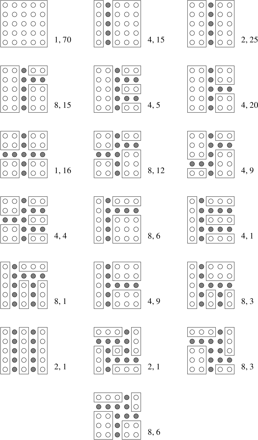
Now we begin the proof of Theorem 2.3 with a sequence of lemmas. The first one concerns the first property in Definition 2.2 and is taken from Lemma 3.3 in [11].

Lemma 2.5

The corner variables $x_{11}$ , $x_{1n}$ , $x_{m1}$ , and $x_{mn}$ do not belong to $S_{P}$ for any minimal prime $P$ of $I_{mn}(2)$ .

Lemma 2.6

If $P$ is a minimal prime of $I_{mn}(2)$ , then every maximally connected subset of $N_{P}$ is a rectangle.

Proof. Let $T$ be a maximally connected subset of $N_{P}$ and suppose that the adjacent variables $x_{ij}$ and $x_{i+1,j+1}$ are in $T$ . Since these two variables are not in $P$ , the only way the adjacent minor $x_{ij}x_{i+1,j+1}-x_{i,j+1}x_{i+1,j}$ could be in $P$ is if the variables $x_{i+1,j}$ and $x_{i,j+1}$ also belong to $N_{P}$ . Since $T$ is maximally connected these two variables are also in $T$ . Similarly, if $x_{i+1,j}$ and $x_{i,j+1}$ belong to $T$ then $x_{ij}$ and $x_{i+1,j+1}$ are also in $T$ . This implies that any maximally connected subset of $N_{P}$ is a rectangle. $\Box$

The general description of the minimal primes in (1) together with Lemma 2.6 imply that if $P$ is a minimal prime of $I_{mn}(2)$ , and $N_{P}$ , the set of variables not in $P$ , is written as the disjoint union of its maximally connected rectangles, say $N_{P}=\bigcup_{k}T_{k}$ , then

P=\langle x_{ij}:\,\,x_{ij}\in S_{P}\rangle\,+\,\langle x_{ij}x_{st}-x_{it}x_{sj}:\mbox{ all of }x_{ij},x_{st},x_{it},x_{sj}\mbox{ are in the same }T_{k}\rangle.

Lemma 2.7

Let $P$ be a minimal prime of $I_{mn}(2)$ and let $T$ be a maximally connected rectangle of $N_{P}$ . Then the boundary of $T$ is a subset of $S_{P}$ . Moreover, for each boundary edge $E$ of $T$ there is another maximal rectangle $T^{\prime}\subset N_{P}$ whose boundary has a nonempty intersection with $E$ .

Proof. The boundary of $T$ is a subset of $S_{P}$ since $T$ is maximally connected. To prove the second statement, suppose that there were a maximal rectangle $T$ with a boundary edge $E$ that does not intersect the boundary of any other maximal rectangle. Consider the prime ideal $P^{\prime}$ where $S_{P^{\prime}}=S_{P}\setminus E$ , and $N_{P^{\prime}}=N_{P}\cup E$ . The assumption on the edge $E$ implies that $T^{\prime}=T\cup E$ is a maximally connected rectangle of $N_{P^{\prime}}$ . The new prime ideal $P^{\prime}$ still contains all the adjacent minors. The only new $2\times 2$ minors that appear in the ideal $P^{\prime}$ involve variables from $E$ , and these are already contained in $P$ . This implies that $P^{\prime}$ is a prime ideal contained in $P$ , contradicting the minimality of $P$ . $\Box$

Lemma 2.8

Let $P$ be a minimal prime of $I_{mn}(2)$ and let $T=X[i,j;i,s]$ be a maximally connected rectangle in $N_{P}$ of height one. Then there is no maximally connected rectangle of height one in $N_{P}$ of the form $T^{\prime}=X[i,s+2;i,t]$ . A similar statement holds for vertical rectangles of width one.

Proof. By Lemma 2.7 the rectangles $X[i-1,j;i-1,t]$ and $X[i+1,j;i+1,t]$ , and the variable $x_{i,s+1}$ are in $S_{P}$ . Since the variables of $T$ and $T^{\prime}$ do not appear in any generator of $P$ , the prime ideal $P^{\prime}$ given by the set of variable $S_{P}\setminus x_{i,s+1}$ is a strictly smaller prime ideal which contains $I_{mn}(2)$ , contradicting the minimality of $P$ . $\Box$

Lemma 2.9

If $P$ is a minimal prime of $I_{mn}(2)$ , then every variable in $S_{P}$ belongs to the boundary of some maximal rectangle in $N_{P}$ .

Proof. Suppose that $S_{P}$ contains a variable $x_{ij}$ that is not in the boundary of any maximal rectangle in $N_{P}$ . This implies that $x_{ij}$ is adjacent only to variables in $S_{P}$ . Let $U\subset S_{P}$ be the set of variables that are adjacent to $x_{ij}$ . The $2\times 2$ adjacent minors contained in the ideal generated by the variables in $U\cup x_{ij}$ are the same as those contained in the ideal generated by the variables in $U$ alone. Hence by omitting the variable $x_{ij}$ from $P$ we can construct a prime ideal that contains $I_{mn}(2)$ , but strictly contained in $P$ . This is a contradiction to the minimality of $P$ . $\Box$

With the help of the five lemmas we have presented we are ready to prove the main theorem of this section.

Proof of Theorem 2.3. If $P$ is a minimal prime of $I_{mn}(2)$ , the partition $(S_{P},N_{P})$ satisfies all the five properties to be a prime partition because of the five lemmas, Lemma 2.5 through Lemma 2.9, above. Hence we just need to prove the converse. Suppose $(S,N)$ is a prime partition, and we assume $N=\cup_{k}T_{k}$ is the partition of $N$ into its maximally connected rectangles. We will show that the prime ideal

P=\langle x_{ij}:\,\,x_{ij}\in S\rangle\,+\,\langle x_{ij}x_{st}-x_{it}x_{sj}:\mbox{ all of }x_{ij},x_{st},x_{it},x_{sj}\mbox{ are in the same }T_{k}\rangle

is a minimal prime of $I_{mn}(2)$ . Since all the $T_{k}$ are rectangles, it is easy to see that $P$ contains $I_{mn}(2)$ . Suppose that there were a minimal prime $P^{\prime}$ over $I_{mn}(2)$ strictly contained in $P$ . This means that $(S_{P^{\prime}},N_{P^{\prime}})$ is a prime partition, and $S_{P^{\prime}}$ is a proper subset of $S_{P}=S$ . We consider a variable $x_{ij}$ in $S_{P}\setminus S_{P^{\prime}}$ . By Lemma 2.9, $x_{ij}$ lies on the boundary of some maximal rectangle $T$ of $N_{P}=N$ . The variable $x_{ij}$ either lies on a boundary edge $E$ of $T$ , or is a corner variable on the boundary of $T$ . In the first case, since $(S_{P^{\prime}},N_{P^{\prime}})$ is a prime partition, $E\subset S_{P}\setminus S_{P^{\prime}}$ , and therefore $E$ is a subset of $N_{P^{\prime}}$ . Moreoever $E$ intersects the boundary of at least one other rectangle $T^{\prime}$ of $N_{P}$ . This means $T\cup E\cup T^{\prime}$ is a connected subset of $N_{P^{\prime}}$ , and this union must be contained in a maximally connected rectangle $T^{\prime\prime}$ of $N_{P^{\prime}}$ . If $x_{ij}$ is a corner variable of the boundary of $T$ , then the two boundary edges $E$ and $E^{\prime}$ of $T$ that are adjacent to $x_{ij}$ must be a part of $N_{P^{\prime}}$ . Now by repeating the above argument we are guaranteed to have another rectangle $T^{\prime}$ of $N_{P}$ where $T\cup E\cup T^{\prime}$ is contained in a maximally connected rectangle $T^{\prime\prime}$ of $N_{P^{\prime}}$ . By the fourth property of Definition 2.2, $T$ and $T^{\prime}$ could not be both height (width) one rectangles in the same row (column) of $X_{mn}$ . Hence there are variables $x_{st}\in T$ and $x_{pq}\in T^{\prime}$ where $s\neq p$ and $t\neq q$ . Since these variables are in the same maximally connected rectangle $T^{\prime\prime}$ of $N_{P^{\prime}}$ , the $2\times 2$ minor $x_{st}x_{pq}-x_{sq}x_{pt}$ is in $P^{\prime}$ . On the other hand, the set of variables appearing in this minor is not contained in any maximally connect rectangle of $N_{P}$ and so it does not belong to $P$ . This contradicts the assumption that $P^{\prime}\subset P$ . $\Box$

There are many open questions left to answer about $I_{mn}(2)$ . A combinatorial description of the embedded primes remains elusive. Moreover, there are many interesting open questions regarding the minimal primes. For example, how many are there, which minimal primes have the largest dimension, and what is the degree of the radical $\mathrm{rad}(I_{mn}(2))$ ?

3 Maximal Adjacent Minors

In this section we will describe the complete primary decomposition of the ideals $I_{mn}(m)$ for $m\leq n$ over a field $K$ of characteristic zero, and for $m\leq 3$ in arbitrary characteristic. With no restrictions on the characteristic of the field our description presents $I_{mn}(m)$ as the irredundant intersection of radical ideals.

Proposition 3.1

The ideal $I_{mn}(m)$ is a radical ideal that is a complete intersection. Its codimension is $n-m+1$ and it has degree $m^{n-m+1}$ .

Proof. With respect to the lexicographic term order where $x_{11}\succ x_{12}\succ\cdots\succ x_{1n}\succ x_{21}\succ\cdots\succ x_{mn}$ , the set of $m\times m$ adjacent minors of $X_{mn}$ is a Gröbner basis of $I_{mn}(m)$ . This follows from the fact that the initial terms of these minors are pairwise relatively prime. The initial ideal is a radical ideal that is a complete intersection, and hence so is $I_{mn}(m)$ . Since there are $n-m+1$ maximal adjacent minors, the codimension of $I_{mn}(m)$ is $n-m+1$ and its degree is $m^{n-m+1}$ . $\Box$

Below we will give a description of the minimal primes of $I_{mn}(m)$ . In this section we will show that $I_{mn}(m)$ is the irredundant intersection of these radical ideals. The proof that they are prime in characteristic zero and when $m\leq 3$ for arbitrary characteristic occupies Section 4.

Description of the minimal primes

In order to make the narrative cleaner we will assume that the matrix $X_{mn}$ has two phantom columns: a column indexed by $0$ and another by $n+1$ . (The role of the phantom columns is only to make the description of the minimal primes simpler.) We will denote by $[i,j]$ with $0\leq i\leq j\leq n+1$ the interval of column indices $\{i,i+1,\ldots,j-1,j\}$ of $X_{mn}$ , and $X[i,j]$ will denote the submatrix consisting of the corresponding columns of $X_{mn}$ .

Definition 3.2

Let $\Gamma=\{[a_{1},b_{1}],[a_{2},b_{2}],\ldots,[a_{k},b_{k}]\}$ be a sequence of $k$ intervals. The sequence $\Gamma$ is called a prime sequence if it satisfies the following properties:

1.

$\bigcup[a_{i},b_{i}]=[0,n+1]$ ,
2.

$a_{i}<a_{i+1}$ , $b_{i}<b_{i+1}$ for all $i$ ,
3.

$b_{i}-a_{i}>m$ for all $i$ , and
4.

$0\leq b_{i}-a_{i+1}<m-1$ for all $i$ .

The definition says that each interval of $\Gamma$ is a block of more than $m$ columns and all together they cover all the columns of $X_{mn}$ (including the two phantom columns). Moreover the consecutive intervals in the sequence have a nonempty overlap of width less than $m$ . Given a prime sequence $\Gamma$ we let $P_{\Gamma}$ be the ideal in $K[x_{ij}]$ defined by

1.

all $m\times m$ minors of $X[a_{i},b_{i}]$ for each $[a_{i},b_{i}]\in\Gamma$ , and
2.

all (maximal) $(b_{i}-a_{i+1}+1)\times(b_{i}-a_{i+1}+1)$ minors of $X[a_{i+1},b_{i}]$ for $1\leq i\leq k-1$ .

In other words, $P_{\Gamma}$ is generated by the $m\times m$ minors of the submatrices whose columns are indexed by the intervals in $\Gamma$ , and the maximal minors of the submatrices whose columns are indexed by the overlap of consecutive intervals. An example will do the best job to illustrate this construction.

Example 3.3

We display the minimal primes $P_{\Gamma}$ of $I_{36}(3)$ . There are seven primes corresponding to the seven prime sequences:

\begin{array}[]{rcl}\Gamma_{1}&=&\{[0,7]\}\\ \Gamma_{2}&=&\{[0,3],[3,7]\}\\ \Gamma_{3}&=&\{[0,3],[2,7]\}\\ \Gamma_{4}&=&\{[0,4],[4,7]\}\\ \Gamma_{5}&=&\{[0,4],[3,7]\}\\ \Gamma_{6}&=&\{[0,5],[4,7]\}\\ \Gamma_{7}&=&\{[0,3],[2,6],[4,7]\}\end{array}

Figure 3 illustrates these minimal primes. The rectangles with the solid borders describe the intervals in the corresponding prime sequence. All $3\times 3$ minors of each rectangle are included in the corresponding minimal prime. We also indicate the overlaps by rectangles with dashed borders; all the maximal minors in these submatrices also need to be included in the corresponding minimal prime. $\Box$

The Main Theorem

We now present the proof that the ideals $P_{\Gamma}$ describe the prime decomposition of $I_{mn}(m)$ in characteristic zero and when $m\leq 3$ . The following lemma will be needed for the proof of Theorem 3.5.

Lemma 3.4

The variety $\mathcal{V}(I_{mn}(m))$ is contained in $\bigcup\mathcal{V}(P_{\Gamma})$ where the union is taken over all prime sequences of $[0,n+1]$ .

Proof. We will show that for each matrix $\mathbf{X}\in\mathcal{V}(I_{mn}(m))$ there is a prime sequence $\Gamma$ such that $\mathbf{X}\in\mathcal{V}(P_{\Gamma})$ . We describe an algorithm that constructs this prime sequence $\Gamma$ . For this, let $\mathcal{I}(\mathbf{X}):=\{[c_{1},d_{1}],\ldots,[c_{t},d_{t}]\}$ be the set of all intervals of width less than $m$ in $[1,n]$ such that $\mathbf{X}[c_{i},d_{i}]$ has rank $d_{i}-c_{i}$ , and $[c_{i},d_{i}]\not\subset[c_{j},d_{j}]$ for $i\neq j$ . We assume that $c_{1}<\cdots<c_{t}$ . We define a prime sequence $\Gamma$ as follows:

1.

Set $i=a_{1}=b_{0}=0$ and $\Gamma=\emptyset$ .
2.
While $b_{i}\neq n+1$ do
- (a)
  
  i := i + 1.
- (b)
  
  Let $[c_{j_{i}},d_{j_{i}}]\in\mathcal{I}(\mathbf{X})$ be the first interval in $[a_{i},n+1]$ with $c_{j_{i}}>a_{i}+1$ . If there is no such interval set $b_{i}=n+1$ .
- (c)
  
  If $d_{j_{i}}\leq a_{i}+m$ set $b_{i}=a_{i}+m$ , unless $a_{i}+m\geq n$ in which case set $b_{i}=n+1$ . Otherwise set $b_{i}=d_{j_{i}}$ .
- (d)
  
  $\Gamma:=\Gamma\cup\{[a_{i},b_{i}]\}$ .
- (e)
  
  If $b_{i}\neq n+1$ , let $[p_{j_{i}},q_{j_{i}}]\in\mathcal{I}(\mathbf{X})$ be the last interval in $[a_{i},b_{i}]$ . Set $a_{i+1}=p_{j_{i}}$ .
3.

If the last interval in $\Gamma$ has width less than $m+1$ replace it with $[n+1-m,n+1]$ .

Step $2\mathrm{(c)}$ together with step $3$ guarantees that the intervals in $\Gamma$ have width at least $m+1$ . Moreover, step $2\mathrm{(e)}$ implies that consecutive intervals have a nonempty overlap of width less than $m$ . These show that $\Gamma$ is a prime sequence.

Next we show that $\mathbf{X}$ is in $\mathcal{V}(P_{\Gamma})$ . By the above construction of $\Gamma$ the overlap $[a_{i+1},b_{i}]$ of two consecutive intervals contains one of the elements $[c_{i},d_{i}]$ of $\mathcal{I}(\mathbf{X})$ . Since $\mathbf{X}[c_{i},d_{i}]$ is rank-deficient (it has rank $d_{i}-c_{i}$ instead of $d_{i}-c_{i}+1$ ), so is $\mathbf{X}[a_{i+1},b_{i}]$ , and the corresponding $(b_{i}-a_{i+1}+1)\times(b_{i}-a_{i+1}+1)$ minors vanish on $\mathbf{X}$ .

We need to show that the rank of $\mathbf{X}[a_{i},b_{i}]$ for each $[a_{i},b_{i}]\in\Gamma$ is at most $m-1$ . For this we analyze a few different cases. First suppose that the width of $[a_{i},b_{i}]$ is bigger than $m+1$ . The above algorithm implies that there are either zero, one, two, or three intervals from $\mathcal{I}(\mathbf{X})$ that are in $[a_{i},b_{i}]$ . When there are no such intervals then $\Gamma=\{[0,n+1]\}$ , and the matrix $\mathbf{X}$ does not have any rank-deficient submatrices consisting of less than $m$ adjacent columns. So $\mathbf{X}[1,m-1]$ has full rank and these columns generate a subspace $V$ with $\dim(V)=m-1$ . But since the span of $\mathbf{X}[1,m]$ is also $V$ and $\mathbf{X}[2,m]$ has rank $m-1$ , the span of $\mathbf{X}[2,m+1]$ and hence the span of $\mathbf{X}[1,m+1]$ is $V$ . Now by induction it is easy to see that the span of $\mathbf{X}$ is the $(m-1)$ -dimensional space $V$ , and therefore all $m\times m$ minors vanish on $\mathbf{X}$ . If there is one interval from $\mathcal{I}(\mathbf{X})$ inside $[a_{i},b_{i}]$ , then either $[a_{i},b_{i}]=[a_{i},n+1]$ and the only minimal rank-deficient interval is of the form $[a_{i},c]$ with $c<n$ , or $[a_{i},b_{i}]=[0,b_{i}]$ and the only minimal rank-deficient interval is of the form $[c,b_{i}]$ with $c>1$ . In the first case, the submatrix $\mathbf{X}[a_{i}+1,n]$ has at least $m$ columns, and this matrix does not have any rank-deficient submatrices consisting of less than $m$ adjacent columns. By the same argument above we conclude that the span of $\mathbf{X}[a_{i}+1,n]$ is an $(m-1)$ -dimensional subspace $V$ . But since $\mathbf{X}[a_{i},c]$ is minimally rank-deficient we conclude that the span of $\mathbf{X}[a_{i},n]$ is $V$ , and therefore all $m\times m$ minors corresponding to this interval vanish on $\mathbf{X}$ . A symmetric argument applies when $[a_{i},b_{i}]=[0,b_{i}]$ .

In the case where there are two intervals from $\mathcal{I}(\mathbf{X})$ , the two minimally rank-deficient intervals are of the form $[a_{i},c]$ and $[d,b_{i}]$ where $c<b_{i}$ and $d>a_{i}$ or of the form $[a_{i},c]$ and $[a_{i}+1,d]$ which forces the interval $[a_{i},b_{i}]=[a_{i},n+1]$ . This means that, in the first case, $\mathbf{X}[a_{i}+1,b_{i}-1]$ has at least $m$ columns and does not have any rank-deficient submatrices consisting of less than $m$ adjacent columns. Similar considerations as above show that $\mathbf{X}[a_{i}+1,b_{i}-1]$ has rank $m-1$ . Since $\mathbf{X}[a_{i},c]$ is minimally rank deficient and $\mathbf{X}[a_{i}+1,a_{i}+m]$ is not rank deficient we see that the column of $\mathbf{X}$ indexed by $a_{i}$ is in the span of the columns of $\mathbf{X}[a_{i}+1,a_{i}+m]$ and so $\mathbf{X}[a_{i},b_{i}]$ has rank $m-1$ . In the second case, the usual argument implies that $\mathbf{X}[a_{i}+1,n]$ has rank $m-1$ . But since $\mathbf{X}[a_{i},c]$ is minimally rank deficient and $\mathbf{X}[a_{i}+1,c]$ is not rank deficient we see that the column of $\mathbf{X}$ indexed by $a_{i}$ is in the span of the columns of $\mathbf{X}[a_{i}+1,n]$ and so $\mathbf{X}[a_{i},n]$ has rank $m-1$ . Finally, we consider the case where there are three intervals from $\mathcal{I}(\mathbf{X})$ in $[a_{i},b_{i}]$ . By construction these are necessarily of the form $[a_{i},c],[a_{i}+1,d]$ , and $[e,b_{i}]$ . But then the combination of the two arguments for the cases with two minimally rank deficient intervals shows that $\mathbf{X}[a_{i},b_{i}]$ has rank $m-1$ .

The case where the width of $[a_{i},b_{i}]$ is exactly $m+1$ requires a slightly different argument. If $[a_{i},b_{i}]=[0,m]$ or $[n+1-m,n+1]$ there is nothing to show since there is only one $m\times m$ minor that needs to be considered and it is necessarily an adjacent minor. If we are not in these two trivial cases, the construction of $\Gamma$ implies that there are at least two intervals from $\mathcal{I}(\mathbf{X})$ contained in $[a_{i},b_{i}]$ . Let $[c,d]$ be the first such interval and $[e,f]$ the last such interval. Observe that we have $c=a_{i}$ . Now if these two intervals do not overlap then any $m\times m$ submatrix of $\mathbf{X}[a_{i},b_{i}]$ will contain one of these rank-deficient intervals and hence its rank will be at most $m-1$ . If there is an overlap we have $a_{i}<e\leq d<f\leq b_{i}$ . The rank of the submatrix $\mathbf{X}[a_{i},d]$ is $d-a_{i}$ , and the rank of $\mathbf{X}[e,f]$ is $f-e$ . Moreover, since these intervals are minimally rank-deficient the rank of $\mathbf{X}[e,d]$ is $d-e+1$ . But then the rank of $\mathbf{X}[a_{i},b_{i}]$ is at most

(d-a_{i})+(f-e)-(d-e+1)+(b_{i}-f)=b_{i}-a_{i}-1=m-1.

This completes the proof of the lemma. $\Box$

Theorem 3.5

Let $K$ be a field of arbitrary characteristic. Then the ideal of adjacent minors $I_{mn}(m)$ can be written as the irredundant intersection of radical ideals

I_{mn}(m)=\bigcap P_{\Gamma}

where the intersection runs over all prime sequences of $[0,n+1]$ . When $char(K)=0$ or when $m\leq 3$ in arbitrary characteristic this is a minimal prime decomposition.

Proof. Since $P_{\Gamma}$ is radical by Corollary 4.5, the intersection $\bigcap P_{\Gamma}$ is also radical. Moreover, given any prime sequence $\Gamma$ , each adjacent $m\times m$ minor belongs to $P_{\Gamma}$ since the column indices of this minor are either contained in an interval $[a_{i},b_{i}]$ in $\Gamma$ or they contain the indices of one of the overlaps $[a_{i+1},b_{i}]$ . This shows that $I_{mn}(m)$ is contained in this radical ideal. If $K$ is algebraically closed, Lemma 3.4 and the Nullstellensatz imply that $I_{mn}(m)$ is equal to the intersection. Since all the ideals in question lie in $K[x_{ij}]$ for any field $K$ we deduce that the equation holds over any field by passing to the algebraic closure. In order to prove that this intersection is irredundant we need to argue that if $\Gamma\neq\Gamma^{\prime}$ then $P_{\Gamma}$ and $P_{\Gamma^{\prime}}$ are incomparable. This is a consequence of our Gröbner basis arguments and is proven in Corollary 4.6. The intersection is a prime decomposition in characteristic zero because $P_{\Gamma}$ is prime when $\mathrm{char}(K)=0$ : this is the content of Theorem 4.20. Similarly, all the ideals $P_{\Gamma}$ are prime when $m\leq 3$ and the characteristic is arbitrary. This is proven in Corollary 4.15. $\Box$

Theorem 3.6

Let $f_{m}(n)$ be the number of primes in the prime decomposition of $I_{mn}(m)$ . Then $f_{m}(n)$ is generated by the following recurrence:

f_{m}(n+1)=\sum_{i=0}^{m-1}f_{m}(n-i)

subject to the initial conditions $f_{m}(1)=f_{m}(2)=\cdots=f_{m}(m-2)=0$ , $f_{m}(m-1)=1$ and $f_{m}(m)=1$ .

Proof. We count the prime sequences $\Gamma$ on $[0,n+1]$ . There are no such sequences when $n<m-1$ and there is a unique sequence when $n=m-1$ or $n=m$ . If the last interval $[a_{i},n+1]$ in $\Gamma$ has width greater than $m+1$ then $\Gamma^{\prime}=\Gamma-[a_{i},n+1]\cup[a_{i},n]$ is a prime sequence of $[0,n]$ . If the width of $[a_{i},n+1]$ is $m+1$ , then $\Gamma^{\prime}=\Gamma-[a_{i},n+1]$ is a prime sequence of $[0,n+1-j]$ for $2\leq j\leq m$ . This gives an injective map from the set of prime sequences of $[0,n+1]$ to the disjoint union of prime sequences of $[0,n+1-m],[0,n+2-m],\ldots,[0,n]$ . It is also easy to see that the inverse of this map is injective. Hence these two sets have the same cardinality which proves the theorem. $\Box$

4 A new class of prime determinantal ideals

We now prove that the ideals $P_{\Gamma}$ are prime ideals in characteristic zero. We believe they are prime in arbitrary characteristic and we verify this conjecture in special cases. First we will show that $P_{\Gamma}$ is a radical ideal through a Gröbner basis argument which does not depend on $\mathrm{char}(K)$ . Then we use an intricate geometric argument to show that $\mathcal{V}(P_{\Gamma})$ is irreducible over fields of characteristic zero.

A Gröbner basis

We will use the diagonal term order introduced in Proposition 3.1. The argument will also depend on the following lemma proved in [4].

Lemma 4.1

Let $I$ and $J$ be two homogeneous ideals of a polynomial ring $K[x_{1},\ldots,x_{n}]$ , and let $F$ and $G$ be Gröbner bases of $I$ and $J$ with respect to a fixed term order $\prec$ . Then $F\cup G$ is a Gröbner basis of $I+J$ with respect to $\prec$ if and only if for every $f\in F$ and $g\in G$ there exists $h\in I\cap J$ such that $\mathrm{in}(h)=\mathrm{LCM}(\mathrm{in}(f),\mathrm{in}(g))$ .

Our main Gröbner basis result follows from the result below.

Lemma 4.2

Let $F$ be the set of $m\times m$ minors of $X_{mn}$ and let $G$ be the set of the $k\times k$ minors of the submatrix which consists of either the first or the last $k$ columns of $X_{mn}$ where $k<m$ . Then with respect to the lexicographic term order $x_{11}\succ x_{12}\succ\cdots\succ x_{1n}\succ\cdots\succ x_{mn}$ the set $F\cup G$ is a Gröbner basis of the ideal it generates.

Proof. We prove the case where $G$ is the set of the $k\times k$ minors of the submatrix $Y$ consisting of the first $k$ columns of $X_{mn}$ since the other case follows from a symmetric argument similar to the one we give below. We will use Lemma 4.1 where $I=\langle F\rangle$ and $J=\langle G\rangle$ . Note that $F$ and $G$ are Gröbner bases for $I$ and $J$ with respect to the given term order by [14]. For $f\in F$ and $g\in G$ we want to show that there is $h\in I\cap J$ such that $\mathrm{in}(h)=\mathrm{LCM}(\mathrm{in}(f),\mathrm{in}(g))$ . We will construct $h$ as follows: let $\mathrm{in}(f)=x_{1i_{1}}x_{2i_{2}}\cdots x_{mi_{m}}$ where $1\leq i_{1}<i_{2}<\cdots<i_{m}\leq n$ , and let $\mathrm{in}(g)=x_{j_{1}1}x_{j_{2}2}\cdots x_{j_{k}k}$ where $1\leq j_{1}<j_{2}<\cdots<j_{k}\leq m$ . It is not hard to see that if $\mathrm{in}(f)$ contains a variable $x_{si_{s}}$ where $i_{s}\leq k$ then for the corresponding variable $x_{j_{i_{s}}i_{s}}$ of $\mathrm{in}(g)$ we have $j_{i_{s}}\geq s$ . Let $Y_{1}$ be the set of columns of $Y$ indexed by the $j_{t}$ with $j_{i_{s}}=s$ , and let $Y_{2}$ be the set of those columns of $Y$ indexed by those $j_{t}$ which have $j_{i_{s}}>s$ . Moreover, let $Y_{3}$ be the set of columns that do not contain a variable from $\mathrm{in}(f)$ ; that is, $Y_{3}$ consists of the columns of $Y$ which are not in $Y_{1}$ or $Y_{2}$ . Finally, $Y_{4}$ will be the set of columns of $X_{mn}$ with indices $\{i_{t}:\,i_{t}>k\}$ . We make two simple observations. First of all, the sum $|Y_{1}|+|Y_{2}|+|Y_{4}|$ is equal to $m$ , and secondly, $Y_{1}$ comes before all of the other $Y_{i}$ in $X_{mn}$ : indeed, $Y_{1}$ is the first $|Y_{1}|$ columns of $X_{mn}$ . Now let us look at the rows of $Y$ in which a variable of $\mathrm{in}(g)$ that is also either in $Y_{2}$ or $Y_{3}$ appears. These rows form a $(|Y_{2}|+|Y_{3}|)\times k$ submatrix of $Y$ that we will denote by $A$ . With all this data we construct the $(m+|Y_{2}|+|Y_{3}|)\times(m+|Y_{2}|+|Y_{3}|)$ matrix

\left[\begin{array}[]{c|c}A&0\\ \hline\cr Y&Y_{2}\,|\,Y_{4}\end{array}\right],

and we let $h$ be its determinant. Since $h$ can be computed by the Laplace expansion either using the $m\times m$ minors of the last $m$ rows, or using the $k\times k$ minors of the first $k$ columns we deduce that $h$ is in $I\cap J$ . The specific term order we use together with the second observation above gives us the fact that $\mathrm{in}(h)=\mathrm{LCM}(\mathrm{in}(f),\mathrm{in}(g))$ . This is the easiest to see by computing the Laplace expansion using the first $|Y_{2}|+|Y_{3}|$ rows of the matrix. $\Box$

Example 4.3

The proof of Lemma 4.2 relies on the construction of a special element $h$ in $I\cap J$ . We will now describe an example of this construction in the case $m=5$ , $n=6$ , and $k=3$ and we will suppose that we are taking $3\times 3$ minors from the last three columns of $X_{mn}$ . In other words, we illustrate the symmetrical case that we omitted in the above proof. We will consider the special case where $f$ is the $5\times 5$ minor with column indices $\{1,2,3,4,6\}$ and $g$ is the $3\times 3$ minor with row indices $\{2,3,5\}$ . We can represent the situation pictorially with a marked matrix: the crosses $\times$ represent variables which appear in the leading term of $f$ and the squares $\Box$ represent variables which appear in the leading term of $g$ . Our marked matrix is

\left[\begin{array}[]{ccc|ccc}\times&&&&&\\ &\times&&\Box&&\\ &&\times&&\Box&\\ &&&\times&&\\ &&&&&\!\boxtimes\end{array}\right].

According to the symmetric version of the construction, we take $Y_{1}$ to consist of the last column of the matrix, $Y_{2}$ is the third to last column, $Y_{3}$ is the second to last column, and $Y_{4}$ consists of the first three columns. We construct the new matrix whose determinant is the desired polynomial $h$ . In this new matrix, we again use symbols to mark the desired variables in the leading term. This new matrix is a $7\times 7$ matrix and looks like

\left[\begin{array}[]{cccc|ccc}0&0&0&0&\Box&&\\ 0&0&0&0&&\Box&\\ \hline\cr\times&&&&&&\\ &\times&&\Box&\Box&&\\ &&\times&&&\Box&\\ &&&\times&\times&&\\ &&&&&&\!\boxtimes\end{array}\right].

It is easy to see that $\mathsf{in}(h)=\mathrm{LCM}(\mathsf{in}(f),\mathsf{in}(g))$ : just use the Laplace expansion along the first two rows. $\Box$

Theorem 4.4

With respect to the lexicographic term order $x_{11}\succ x_{12}\succ\cdots\succ x_{1n}\succ\cdots\succ x_{mn}$ all the minors defining $P_{\Gamma}$ form a Gröbner basis.

Proof. We do induction on the number of intervals in $\Gamma=\{[a_{1},b_{1}],\ldots,[a_{t},b_{t}]\}$ . If $\Gamma=\{[0,n+1]\}$ , then $P_{\Gamma}$ is just generated by the $m\times m$ minors of $X_{mn}$ and by the results in [14] they form a Gröbner basis. When there is more than one interval then $\Gamma^{\prime}=\Gamma-[a_{t},n+1]$ is a prime sequence for $[0,b_{t-1}+1]$ . By induction, the set of minors $F$ generating $P_{\Gamma^{\prime}}$ is a Gröbner basis of $I:=I_{mb_{t-1}}(m)$ . Now we let $J$ be the ideal generated by the $m\times m$ minors corresponding to the interval $[a_{t},b_{t}]$ and the maximal minors of the overlap $[a_{t},b_{t-1}]$ . We let $k:=b_{t-1}-a_{t}+1$ , and we denote the set of these $k\times k$ minors together with the $m\times m$ minors that generate $J$ by $G$ . Lemma 4.2 implies that $G$ is a Gröbner basis of $J$ . Now we will use Lemma 4.1 to prove the theorem. Observe that if $f\in F$ and $g\in G$ are minors of submatrices corresponding to intervals or overlaps of intervals which do not share a column, then $\mathrm{LCM}(\mathrm{in}(f),\mathrm{in}(g))=\mathrm{in}(f)\cdot\mathrm{in}(g)$ and we choose $h=f\cdot g$ . Hence we only need to study the pairs of intervals that do overlap. Here is the list of the cases we need to consider:

(a)

both $f$ and $g$ are $m\times m$ minors,
(b)

$f$ is an $s\times s$ minor coming from an overlap that also intersects the interval $[a_{t},n+1]$ , and $g$ is an $m\times m$ minor,
(c)

$f$ is as in (b), and $g$ is a $k\times k$ minor,
(d)

$f$ is an $m\times m$ minor coming from an interval that is not $[a_{t-1},b_{t-1}]$ and $g$ is $k\times k$ minor, and
(e)

$f$ is an $m\times m$ minor coming from $[a_{t-1},b_{t-1}]$ and $g$ is a $k\times k$ minor.

The last case is covered by the proof of Lemma 4.2. In all the other cases, simple arguments show that the leading terms of $f$ and $g$ are relatively prime and hence we choose $h=f\cdot g$ . For completeness, we go through this argument for case (c). The main tool is the following simple observation. For any maximal minor of any matrix, the leading term selected by our diagonal lexicographic term order has all of its variables lying in the parallelogram-shaped region bounded by the diagonal extending from the upper left hand corner of the matrix and the diagonal extending from the lower right hand corner. Since $\Gamma$ is a prime sequence, the smallest interval $[a,b]$ which contains the column indices of both $f$ and $g$ has width greater than or equal to $m+1$ . This ensures that the two regions corresponding to the possible variables in the leading terms of these minors do not intersect, because the diagonal from the upper left corner of $X[a,b]$ is below the diagonal from the lower right corner of $X[a,b]$ . This guarantees that the leading terms of $f$ and $g$ are relatively prime as desired. $\Box$

Corollary 4.5

The ideal $P_{\Gamma}$ is radical.

Proof. The initial ideal of $P_{\Gamma}$ given by Theorem 4.4 is squarefree, and therefore it is radical. Then $P_{\Gamma}$ is also radical. $\Box$

Corollary 4.6

If $\Gamma\neq\Gamma^{\prime}$ then $P_{\Gamma}$ and $P_{\Gamma^{\prime}}$ are incomparable.

Proof. We will show that $P_{\Gamma}$ is not contained in $P_{\Gamma^{\prime}}$ . For this it suffices to show that there is a minor among the generators of $P_{\Gamma}$ which is not contained in $P_{\Gamma^{\prime}}$ . Let $[a_{i},b_{i}]$ be the first interval of $\Gamma$ which is not contained in $\Gamma^{\prime}$ and let $[c_{i},d_{i}]$ be the corresponding $i$ th interval of $\Gamma^{\prime}$ . The intervals $[a_{1},b_{1}],\ldots[a_{i-1},b_{i-1}]$ are the first $i-1$ intervals which are common to both $\Gamma$ and $\Gamma^{\prime}$ . There are a few cases to consider.

If $i=1$ then $[a_{1},b_{1}]=[0,b_{1}]$ and $[c_{1},d_{1}]=[0,d_{1}]$ . Suppose that $b_{1}>d_{1}$ . Among the indices in the interval $[d_{1}+1,b_{1}]$ there exists at least one index $e$ so that $[e,e]$ is not an interval obtained by overlapping two consecutive intervals in $\Gamma^{\prime}$ . Then the $m\times m$ minor with columns indices $\{1,\ldots,m-1,e\}$ is contained in $P_{\Gamma}$ but not in $P_{\Gamma^{\prime}}$ because its leading term is not divisible by any leading term in the Gröbner basis for $P_{\Gamma^{\prime}}$ . If we suppose that $b_{1}<d_{1}$ , then any $(b_{1}-a_{2}+1)\times(b_{1}-a_{2}+1)$ minor with column indices $[a_{2},b_{1}]$ belongs to $P_{\Gamma}$ but not $P_{\Gamma^{\prime}}$ since its leading term is not divisible by any leading term in the Gröbner basis for $P_{\Gamma^{\prime}}$ .

Now we suppose that $i>1$ . The arguments are similar to those in the preceding paragraph and we sketch them briefly. Suppose $a_{i}<c_{i}$ . Then there is an $m\times m$ minor with column indices in $[a_{i},b_{i}]$ using the column index $a_{i}$ which is contained in $P_{\Gamma}$ but not $P_{\Gamma}^{\prime}$ . If $a_{i}>c_{i}$ then there is an $(b_{i-1}-a_{i}+1)\times(b_{i-1}-a_{i}+1)$ minor with column indices equal to $[a_{i},b_{i-1}]$ which is contained in $P_{\Gamma}$ but not $P_{\Gamma^{\prime}}$ . Finally, if $a_{i}=c_{i}$ then a minor modification of the $i=1$ case shows that $P_{\Gamma}$ contains a minor which is not contained in $P_{\Gamma^{\prime}}$ . $\Box$

$\mathcal{V}(P_{\Gamma})$ is irreducible

Before proceeding with the proof, we will outline the strategy that we will employ to show that $\mathcal{V}(P_{\Gamma})$ is irreducible over a field $K$ with $\mathrm{char}(K)=0$ . First, we will construct a morphism from an irreducible variety $\mathcal{X}$ to $\mathcal{V}(P_{\Gamma})$ . Then we will argue that this morphism surjects onto a Zariski open subset $\mathcal{W}$ of $\mathcal{V}(P_{\Gamma})$ when restricted to a Zariski open (and necessarily irreducible) subset $\mathcal{Y}$ of $\mathcal{X}$ . This implies that $\mathcal{W}$ is irreducible. Up to this point the results will be obtained without any assumptions on the characteristic of the field. Then we will assume that $K={\mathbb{C}}$ , and we will show that the closure of $\mathcal{W}$ is equal to $\mathcal{V}(P_{\Gamma})$ which proves that $\mathcal{V}(P_{\Gamma})$ is irreducible. This will require a perturbation argument which we present in the next subsection. Finally, we use standard arguments in the proof of Theorem 4.20 to show that $P_{\Gamma}$ is prime over any field of characteristic zero.

We first define the irreducible variety $\mathcal{X}$ . In order to do this we need to introduce a poset $\mathcal{Q}_{\Gamma}$ associated to a prime sequence $\Gamma$ .

Definition 4.7

Let $\Gamma$ be a prime sequence. The elements of the poset $\mathcal{Q}_{\Gamma}$ are certain subintervals of the intervals in $\Gamma$ which will be defined recursively, and these subintervals are ordered with respect to inclusion. The intervals in $\Gamma$ are the maximal elements of $\mathcal{Q}_{\Gamma}$ , and we sort them with respect to each interval’s starting index, the left border, in ascending order. These will form the elements in row $1$ . The elements in row $2$ are the nonempty subintervals obtained by intersecting two consecutive intervals in row $1$ . We also sort row $2$ in ascending order with respect to the left borders. The subsequent rows are defined recursively: the elements in row $r$ consist of all nonempty intervals that arise from the intersection of two consecutive elements from row $r-1$ . It is clear that every nonmaximal element is covered by exactly two elements (a left and a right parent), and each nonminimal element covers at most two other elements (a left and a right child).

Example 4.8

Let $m=6$ and consider the sequence of intervals

\Gamma\,\,=\,\,\{[0,7],[3,9],[5,11],[7,13],[10,17]\}.

The second row of the poset consists of the overlapping intervals $[3,7],[5,9],[7,11]$ , and $[10,13]$ . The third row is formed by the intervals $[5,7],[7,9]$ , and $[10,11]$ . The fourth and final row of the poset is the interval $[7,7]$ . This poset is illustrated in Figure 4. $\Box$

In order to define $\mathcal{X}$ we need one more piece of information. This will be a positive integer attached to each element of $\mathcal{Q}_{\Gamma}$ .

Definition 4.9

For each $p\in\mathcal{Q}_{\Gamma}$ let

D(p):=\left\{\begin{array}[]{cl}m-1&\mbox{if $p$ is in the first row of }\mathcal{Q}_{\Gamma}\\ w(p)-1&\mbox{ if $p$ is in the second row of }\mathcal{Q}_{\Gamma}\\ w(p)&\mbox{otherwise}\end{array}\right.

where $w(p)$ is the width of the interval $p$ .

Now each element $p\in\mathcal{Q}_{\Gamma}$ will give rise to a general linear group ${G_{\!}L}_{k(p)}$ of invertible $k(p)\times k(p)$ matrices where $k(p)=D(q)-D(q^{\prime})$ , and $q$ is the left parent of $p$ and $q^{\prime}$ is the left child of $p$ . If $p$ does not have a left parent then we set $D(q)=m$ , and if $p$ does not have a left child, then we set $D(q^{\prime})=0$ . Moreover each maximal element $q\in\mathcal{Q}_{\Gamma}$ will give rise to an affine space ${\mathbb{A}}^{\ell(q)}$ , and we define $\ell(q)$ as follows: suppose $q$ corresponds to the interval $[a_{s},b_{s}]$ and let $[a_{s+1},b_{s+1}]$ be the next interval (if there is one). Let $\Lambda:=[a_{s},a_{s+1}-1]$ or $\Lambda:=[a_{s},n]$ if $[a_{s},b_{s}]$ is the last interval. Now for each index $i\in\Lambda$ there is a unique $p(i)\in\mathcal{Q}_{\Gamma}$ which is minimal among all elements containing $i$ . It is an easy exercise to see that $p(i)\in\{p_{0},\ldots,p_{r}\}$ where $p_{0}=q$ and $p_{j+1}$ is the left child of $p_{j}$ . With this we define $\ell(q)=\sum_{i\in\Lambda}D(p(i))$ . Finally we arrive at the variety

\mathcal{X}\,\,:=\,\,\prod_{p\in\mathcal{Q}_{\Gamma}}{G_{\!}L}_{k(p)}\,\,\,\times\,\,\,\prod_{q\,\,maximal}{\mathbb{A}}^{\ell(q)}.

We note that over an infinite field $\mathcal{X}$ is irreducible since it is the product of irreducible varieties.

Next we define a map $\phi$ from $\mathcal{X}$ to ${\mathbb{A}}^{mn}$ , the space of all $m\times n$ matrices. Given a point in $x\in\mathcal{X}$ we will build an $m\times n$ matrix piece by piece using the intervals in $\Gamma$ . We start with the last interval $[a_{t},n+1]$ and the corresponding maximal element $q\in\mathcal{Q}_{\Gamma}$ . Then we build an $m\times|\Lambda|$ matrix $\mathbf{Z}$ as follows: for each $i\in\Lambda$ we set all entries in column $i$ with row indices $D(p(i))+1,D(p(i))+2,\ldots,m$ to zero. There are precisely $\ell(q)$ entries in $\mathbf{Z}$ that are not set to zero yet, and we “plug in” the coordinates of the point $x$ corresponding to ${\mathbb{A}}^{\ell(q)}$ to these entries. We set $\mathbf{X}:=\mathbf{Z}$ . Now let $q=p_{0},p_{1},\ldots,p_{s}$ be the elements of $\mathcal{Q}_{\Gamma}$ such that $p_{j+1}$ is the left child of $p_{j}$ , and let $g_{j}\in{G_{\!}L}_{k(p_{j})}$ be the matrices that could be read off from the corresponding coordinates of $x$ . For $j=0,\ldots,s$ we define $\mathbf{X}:=g_{j}\cdot\mathbf{X}$ recursively, where $g_{j}\cdot\mathbf{X}$ is obtained by multiplying the last $k(p_{j})$ rows of the first $D(q_{j})$ rows of $\mathbf{X}$ , and $q_{j}$ is the left parent of $p_{j}$ (since $D(q_{j})\geq k(p_{j})$ , by the definition of $k(p_{j})$ this makes sense).

After we have gone through the sequence $p_{0},\ldots,p_{s}$ , let the resulting matrix be $\mathbf{Y}$ . Next we move onto the second to last interval $[a_{t-1},b_{t-1}]$ , and using the set $\Lambda$ associated to this interval we build a matrix $\mathbf{Z}$ , and then we set $\mathbf{X}:=[\mathbf{Z}|\mathbf{Y}]$ . Now using the various invertible matrices associated to the sequence of the left children starting from $[a_{t-1},b_{t-1}]$ we repeat this procedure. Clearly the result of this construction is an $m\times n$ matrix. It is also clear that this map is a polynomial map and hence a morphism.

Example 4.10

This is a detailed example displaying the variety $\mathcal{X}$ and the recursive construction of the map $\phi$ . Let $m=4$ and let $\Gamma$ be the prime sequence $\Gamma=\{[0,5],[3,7],[5,10]\}$ . The second row of the poset $\mathcal{Q}_{\Gamma}$ consists of the two intervals $[3,5]$ and $[5,7]$ , and the third row of the poset is the singleton interval $[5,5]$ . According to the construction of $\mathcal{X}$ we have

\mathcal{X}={G_{\!}L}_{4}\times{G_{\!}L}_{3}\times{G_{\!}L}_{2}\times{G_{\!}L}_{2}\times{G_{\!}L}_{2}\times{G_{\!}L}_{2}\times{\mathbb{A}}^{6}\times{\mathbb{A}}^{4}\times{\mathbb{A}}^{11}.

We have ordered the general linear groups and the affine spaces in the reverse of the order in which they are used in the map $\phi$ . This should not be confusing to the reader: the ordering of the general linear groups mimics the right to left order of group actions and the affine spaces are ordered in this way as a reminder that we construct the matrix in the image of $\phi$ from right to left. Now let $x$ be an arbitrary point in the variety $\mathcal{X}$ . We begin with the interval $[5,10]$ , the last interval in $\Gamma$ , and use the affine space ${\mathbb{A}}^{11}$ to construct a $4\times 5$ matrix $\mathbf{Z}$ which looks like

\mathbf{Z}=\left[\begin{array}[]{ccccc}*&*&*&*&*\\ 0&*&*&*&*\\ 0&0&0&*&*\\ 0&0&0&0&0\end{array}\right]

and corresponds to columns 5 through 9 of our eventual completed matrix. We set $\mathbf{X}:=\mathbf{Z}$ . Now we read down the right-most chain in the poset and apply the action of general linear groups accordingly. In particular, we apply $g_{1}\in{G_{\!}L}_{2}$ to the bottom two rows of $\mathbf{X}$ , then $g_{2}\in{G_{\!}L}_{2}$ to the middle two rows of $g_{1}\cdot\mathbf{X}$ , and finally $g_{3}\in{G_{\!}L}_{2}$ to the first two rows of $g_{2}\cdot g_{1}\cdot\mathbf{X}$ . Pictorially, we have

\left[\begin{array}[]{ccccc}*&*&*&*&*\\ 0&*&*&*&*\\ 0&0&0&*&*\\ 0&0&0&0&0\end{array}\right]{g_{1}\atop\longrightarrow}\left[\begin{array}[]{ccccc}*&*&*&*&*\\ 0&*&*&*&*\\ 0&0&0&*&*\\ 0&0&0&*&*\end{array}\right]{g_{2}\atop\longrightarrow}\left[\begin{array}[]{ccccc}*&*&*&*&*\\ 0&*&*&*&*\\ 0&*&*&*&*\\ 0&0&0&*&*\end{array}\right]{g_{3}\atop\longrightarrow}\left[\begin{array}[]{ccccc}*&*&*&*&*\\ *&*&*&*&*\\ 0&*&*&*&*\\ 0&0&0&*&*\end{array}\right].

where the last matrix is the matrix $\mathbf{Y}$ obtained at the end of this iteration of the construction. Now we look at the second to last interval $[3,7]$ in $\Gamma$ . Comparing with the interval $[5,10]$ we see that $\Lambda=[3,4]$ , and we add two new columns $\mathbf{Z}$ to $\mathbf{Y}$ above. These come from our ${\mathbb{A}}^{4}$ to arrive at a matrix $\mathbf{X}:=\left[\mathbf{Z}|\mathbf{Y}\right]$ . Reading the second descending chain in $\mathcal{Q}_{\Gamma}$ we apply $g_{4}\in{G_{\!}L}_{2}$ to the last two rows of $\mathbf{X}$ and then apply $g_{5}\in{G_{\!}L}_{3}$ to the first three rows of $g_{4}\cdot\mathbf{X}$ . Pictorially, this looks like

\left[\begin{array}[]{cc|ccccc}*&*&*&*&*&*&*\\ *&*&*&*&*&*&*\\ 0&0&0&*&*&*&*\\ 0&0&0&0&0&*&*\end{array}\right]{g_{4}\atop\longrightarrow}\left[\begin{array}[]{cc|ccccc}*&*&*&*&*&*&*\\ *&*&*&*&*&*&*\\ 0&0&0&*&*&*&*\\ 0&0&0&*&*&*&*\end{array}\right]{g_{5}\atop\longrightarrow}\left[\begin{array}[]{cc|ccccc}*&*&*&*&*&*&*\\ *&*&*&*&*&*&*\\ *&*&*&*&*&*&*\\ 0&0&0&*&*&*&*\end{array}\right].

And again the last matrix is the matrix $\mathbf{Y}$ obtained at the end of the second iteration of the construction. We are now at the last step and we adjoin two new columns $\mathbf{Z}$ to our matrix $\mathbf{Y}$ . The entries in these columns come from the ${\mathbb{A}}^{6}$ . We form the matrix

\mathbf{X}:=\left[\mathbf{Z}|\mathbf{Y}\right]=\left[\begin{array}[]{cc|ccccccc}*&*&*&*&*&*&*&*&*\\ *&*&*&*&*&*&*&*&*\\ *&*&*&*&*&*&*&*&*\\ 0&0&0&0&0&*&*&*&*\end{array}\right].

Since the interval $[0,5]$ has no left child, we deduce that we should apply $g_{6}\in{G_{\!}L}_{4}$ to the entire matrix. This final matrix $g_{6}\cdot\mathbf{X}$ is the image of $x$ under $\phi$ . $\Box$

Proposition 4.11

The image of $\phi$ is contained in $\mathcal{V}(P_{\Gamma})$ .

Proof. We need to show that for every $x\in\mathcal{X}$ all the minors that generate $P_{\Gamma}$ vanish on $\phi(x)$ . We will prove this by using the definition of $\phi$ . First we observe that if a set of minors vanish on the partial matrix $\mathbf{X}$ in the definition of $\phi$ then after the row operations $g_{j}\cdot\mathbf{X}$ these minors will still vanish on $\mathbf{X}$ . We will show that as we build $\mathbf{X}$ each submatrix of $\mathbf{X}$ that corresponds to $p\in\mathcal{Q}_{\Gamma}$ has rank at most $D(p)$ . This is certainly true after constructing $\mathbf{X}$ corresponding to the last interval of $\Gamma$ , since at most the first $D(p_{j})$ rows of each submatrix corresponding to $p_{j}$ are nonzero. An inductive argument shows that after applying $g_{j}$ to $\mathbf{X}$ , the columns of $\mathbf{X}$ that are in the submatrix corresponding to $p_{k}$ for $k=0,\ldots,j$ , but that are not in the submatrix corresponding to $p_{k+1}$ have nonzero elements in at most the first $D(q_{k})$ rows where $q_{k}$ is the left parent of $p_{k}$ . So when $\mathbf{Y}$ is constructed at most the first $D(q_{j})$ rows of the matrix corresponding to $p_{j}$ for $j=0,\ldots,s$ are nonzero. In order to finish the proof by induction, we assume that after constructing the matrix $\mathbf{Y}$ for an interval in $[a_{r},b_{r}]$ where $r>1$ all the minors arising from the intervals $[a_{r},b_{r}],[a_{r+1},b_{r+1}],\ldots,[a_{t},n+1]$ and their consecutive overlaps vanish on $\mathbf{Y}$ , and in the submatrices corresponding to the sequence $p_{0},\ldots,p_{s}$ (where $p_{0}$ is $[a_{r},b_{r}]$ ) at most the first $D(q_{j})$ rows are nonzero, where $q_{j}$ is the left parent of $p_{j}$ . When we move to the next interval $[a_{r-1},b_{r-1}]$ with the corresponding sequence of elements $\bar{p}_{0},\ldots,\bar{p}_{u}$ , first we consruct $\left[\mathbf{Z}\,|\mathbf{Y}\right]$ . It is easy to see that the submatrix $\mathbf{A}_{j}$ of this matrix corresponding to $\bar{p}_{j}$ is obtained by concatenating the portion of $\mathbf{Z}$ contained in $\mathbf{A}_{j}$ with the submatrix corresponding to the right child of $\bar{p}_{j}$ . Now at most the first $D(\bar{p}_{j})$ rows of the portion of $\mathbf{A}_{j}$ contained in $\mathbf{Z}$ are nonzero, and by induction the same is true for the submatrix corresponding to the right child of $\bar{p}_{j}$ . Hence at most the first $D(\bar{p}_{j})$ rows of $\mathbf{A}_{j}$ are nonzero. This shows that the minors arising from the intervals $[a_{r-1},b_{r-1}],[a_{r},b_{r}],[a_{r+1},b_{r+1}],\ldots,[a_{t},n+1]$ and their consecutive overlaps vanish on $\mathbf{X}:=\left[\mathbf{Z}\,|\mathbf{Y}\right]$ . After applying the row operations $\bar{g}_{j}$ , at most the first $D(\bar{q}_{j})$ rows of the matrix corresponding to $\bar{p}_{j}$ will be nonzero where $\bar{q}_{j}$ is the left parent of $\bar{p}_{j}$ because $k(\bar{p}_{j})=D(\bar{q}_{j})-D(\bar{p}_{j+1})$ . This implies that $\mathbf{X}$ has the properties the induction is based on, and this completes the induction. $\Box$

Now we let $\mathcal{W}$ be the subset of $\mathcal{V}(P_{\Gamma})$ consisting of matrices $\mathbf{X}$ where the rank of each submatrix of $\mathbf{X}$ corresponding to $p\in\mathcal{Q}_{\Gamma}$ is equal to $D(p)$ . Since this subset is defined by the non-vanishing of certain minors we conclude that it is a Zariski open subset of $\mathcal{V}(P_{\Gamma})$ . It is guaranteed to be nonempty by the results in the next subsection. Moreover, we let $\mathcal{Y}$ be the set of $x\in\mathcal{X}$ such that $\phi(x)\in\mathcal{W}$ . We argue that $\mathcal{Y}$ is an open subset of $\mathcal{X}$ . For this, consider an $x\in\mathcal{X}$ where we take the entries as indeterminates. Then $\phi(x)$ is a matrix with polynomial entries in the coordinates of $x$ . Thus $\mathcal{Y}$ is defined by the non-vanishing of certain minors of $\phi(x)$ . Furthermore, $\mathcal{Y}$ is irreducible since $\mathcal{X}$ is irreducible.

Proposition 4.12

The morphism $\phi\,:\,\mathcal{Y}\longrightarrow\mathcal{W}$ is surjective, and therefore $\mathcal{W}$ is irreducible when $K$ is an infinite field.

Proof. Since the second statement follows from the first we just prove the first claim. We will do this by constructing $x\in\mathcal{Y}$ for each $\mathbf{X}\in\mathcal{W}$ such that $\phi(x)=\mathbf{X}$ . We start with the first interval $p=[a_{1},b_{1}]$ in $\Gamma$ . Since $\mathbf{X}[a_{1},b_{1}]$ has rank $D(p)=m-1$ , we can find a $g\in{G_{\!}L}_{k(p)}$ where $k(p)=m$ so that $g\cdot\mathbf{X}[a_{1},b_{1}]$ is row-reduced, in particular, the last row is a zero row. We let $\mathbf{X}=g\cdot\mathbf{X}$ , and we record $g^{-1}$ as well as the entries of the first $D(p)=m-1$ rows of each column of $\mathbf{X}$ with column index $i\in\Lambda$ (see the definition of $\Lambda$ in the paragraph before Example 4.10) as part of the element $x$ we are constructing. Then we delete these columns from $\mathbf{X}$ to obtain the new $\mathbf{X}$ .

By induction, suppose we have gone through the intervals $[a_{1},b_{1}],\ldots,[a_{r-1},b_{r-1}]$ and the matrix $\mathbf{X}=\mathbf{X}[a_{r},n]$ has the following properties. Let $p_{0},p_{1},\ldots,p_{s}$ be the sequence of elements where $p_{0}$ is $[a_{r-1},b_{r-1}]$ and $p_{j+1}$ is the left child of $p_{j}$ . Then the only nonzero rows of the submatrix of $\mathbf{X}$ corresponding to the right child of $p_{j}$ are the first $D(p_{j})$ rows of this submatrix.

Now we let $\bar{p}_{0},\ldots,\bar{p}_{u}$ be the sequence where $\bar{p}_{0}$ is the interval $[a_{r},b_{r}]$ and $\bar{p}_{j+1}$ is the left child of $\bar{p}_{j}$ . We observe that, by induction, only the first $D(\bar{q}_{j})$ rows of the submatrix of $\mathbf{X}$ corresponding to $\bar{p}_{j}$ could be nonzero where $\bar{q}_{j}$ is the left parent of $\bar{p}_{j}$ . Now we apply $\bar{g}_{j}\in{G_{\!}L}_{k(\bar{p}_{j})}$ to $\mathbf{X}$ successively starting from $j=u$ and finishing with $j=0$ . In this process $\bar{g}_{j}$ will be chosen as the matrix which will be applied to the last $k(\bar{p}_{j})$ rows of the first $D(\bar{q}_{j})$ rows of $\mathbf{X}$ so that after applying $\bar{g}_{j}$ , the submatrix of $\mathbf{X}$ corresponding to $\bar{p}_{j}$ is row reduced. Since we have assumed that the submatrix corresponding to $\bar{p}_{j+1}$ has rank equal to $D(\bar{p}_{j+1})$ , this implies that the submatrix corresponding to $\bar{p}_{j}$ with row indices $D(\bar{p}_{j+1})+1$ , $D(\bar{p}_{j+1})+2$ , $\ldots$ , $D(\bar{p}_{j+1})+k(\bar{p}_{j})$ has rank $k(\bar{p}_{j})-1$ . This implies that after applying $\bar{g}_{j}$ the rows indexed by $D(\bar{p}_{j})+1,D(\bar{p}_{j})+2,\ldots,m$ in the submatrix corresponding to $\bar{p}_{j}$ will consist of zeros. Moreover, when applying $\bar{g}_{j}$ , the definition of $k(\bar{p}_{j})$ and the particular rows which will be affected guarantee that the zero rows of the submatrices corresponding to $\bar{p}_{j+1},\ldots,\bar{p}_{u}$ stay as zero rows. Hence when we compute $\mathbf{X}:=\bar{g}_{0}\cdot\mathbf{X}$ , we return to the property we started with at the beginning of the induction step, namely: the only nonzero rows of the submatrix of $\mathbf{X}$ corresponding to $\bar{p}_{j}$ are the first $D(\bar{p}_{j})$ rows of this submatrix.

Now we delete the submatrix $\mathbf{X}[a_{r},a_{r+1}-1]$ from $\mathbf{X}$ to obtain the new $\mathbf{X}$ for the next iteration, and we record the $\ell(\bar{p}_{0})$ possibly nonzero elements in the deleted columns of $\mathbf{X}$ as part of $x$ (this belongs to ${\mathbb{A}}^{\ell(\bar{p}_{0})}$ ) as well as the inverses of all the matrices $\bar{g}_{j}\in{G_{\!}L}_{k(p_{j})}$ which we used. Since we have returned $\mathbf{X}$ to the form of the inductive hypothesis, this shows that we can continue the procedure to compute an $x\in\mathcal{Y}$ whose image under $\phi$ is $\mathbf{X}$ .

$\Box$

We conclude this section with the proof that in certain special cases, the map $\phi:\mathcal{X}\rightarrow\mathcal{V}(P_{\Gamma})$ is, in fact, surjective (i.e. not just surjective on an open subset). Hence, in these cases we may conclude that $P_{\Gamma}$ is prime without resorting to the analytic techniques in Proposition 4.19.

Proposition 4.13

Suppose that $\mathcal{Q}_{\Gamma}$ has only two rows. Then the map $\phi:\mathcal{X}\rightarrow\mathcal{V}(P_{\Gamma})$ is surjective.

Proof. We will closely follow the proof of Proposition 4.12 but with an extra twist. Given an $\mathbf{X}\in\mathcal{V}(P_{\Gamma})$ we will construct $x\in\mathcal{X}$ such that $\phi(x)=\mathbf{X}$ . We start with the first interval $p=[a_{1},b_{1}]$ in $\Gamma$ . Since $\mathbf{X}[a_{1},b_{1}]$ has rank $D(p)=m-1$ , we can find a $g\in{G_{\!}L}_{k(p)}$ where $k(p)=m$ so that $g\cdot\mathbf{X}[a_{1},b_{1}]$ is row-reduced, in particular, the last row is a zero row. We let $\mathbf{X}=g\cdot\mathbf{X}$ , and we record $g^{-1}$ as well as the entries of the first $D(p)=m-1$ rows of each column of $\mathbf{X}$ with column index $i\in\Lambda$ as part of the element $x$ we are constructing. Then we delete these columns from $\mathbf{X}$ to obtain the new $\mathbf{X}$ .

Since $\mathcal{Q}_{\Gamma}$ has only two rows, our inductive hypothesis is simpler than Proposition 4.12. Namely, suppose that we have gone through the intervals $[a_{1},b_{1}],\ldots,[a_{r-1},b_{r-1}]$ and the submatrix of $\mathbf{X}=\mathbf{X}[a_{r},n]$ indexed by $\Lambda=[a_{r},b_{r-1}]$ has its last row as a zero row.

We will let $\bar{p}_{0}=[a_{r},b_{r}]$ and $\bar{p}_{1}=[a_{r},b_{r-1}]$ . Since $\mathcal{Q}_{\Gamma}$ has only two rows, these are the only two elements of $\mathcal{Q}_{\Gamma}$ which we need to consider when we perform our induction. First we use an element of $g_{1}\in{G_{\!}L}_{m-1}$ to row reduce the submatrix consisting of the first $k(\bar{p}_{1})=m-1$ rows of $\mathbf{X}$ and the columns indexed by $\bar{p}_{1}$ . This submatrix has rank $\leq D(\bar{p}_{1})=b_{r-1}-a_{r}$ : if the rank of the submatrix is strictly less than $D(\bar{p}_{1})$ we must perform our row reductions with caution to ensure that the submatrix of $\mathbf{X}$ with columns indexed by $[b_{r-1}+1,b_{r}]$ and consisting of the last $k(\bar{p}_{0})=m-D(\bar{p}_{1})$ rows has rank less than $m-D(\bar{p}_{1})$ . To ensure this possibility, we note that there are two cases to consider. In the first case, the submatrix consisting of its first $m-1$ rows of $\mathbf{X}[a_{r},b_{r}]$ has rank $m-1$ . In this case we can choose $g_{1}$ so that the $(m-1)$ st row of $g_{1}\cdot\mathbf{X}[a_{r},b_{r}]$ is a multiple of the last row of $\mathbf{X}[a_{r},b_{r}]$ . In the second case, the submatrix consisting of the first $m-1$ rows of $\mathbf{X}[a_{r},b_{r}]$ rank $<m-1$ . Then we can choose $g_{1}$ so that the $(m-1)$ st row of $g_{1}\cdot\mathbf{X}[a_{r},b_{r}]$ is the zero row. In either case, this ensures that the last $m-D(\bar{p}_{1})$ rows of $\mathbf{X}[b_{r-1}+1,b_{r}]$ has rank less than $m-D(\bar{p}_{1})$ . Now we apply row reduction via $g_{0}$ in ${G_{\!}L}_{k(\bar{p}_{0})}$ to the last $m-D(\bar{p}_{1})$ rows of $\mathbf{X}$ to bring $\mathbf{X}$ into the form of the inductive hypothesis.

To complete the proof, we record the entries in first $D(\bar{p}_{1})$ rows of $\mathbf{X}[a_{r},b_{r-1}]$ , and the entries in the first $D(\bar{p}_{0})$ rows of $\mathbf{X}[b_{r-1}+1,a_{r+1}-1]$ (this becomes a set of entries in ${\mathbb{A}}^{\ell(\bar{p}_{0})}$ ). We also record the inverses of $g_{1}$ and $g_{0}$ , and we delete the first $|\Lambda|=a_{r+1}-a_{r}$ columns from $\mathbf{X}$ to arrive at $\mathbf{X}:=\mathbf{X}[a_{r+1},n]$ . By our construction, this matrix is in proper form of the inductive hypothesis, and so we may continue the process to construct $x$ such that $\phi(x)=\mathbf{X}$ . $\Box$

Corollary 4.14

Let $K$ be a field of arbitrary characteristic and suppose that $\mathcal{Q}_{\Gamma}$ has only two rows. Then $P_{\Gamma}$ is a prime ideal.

Proof. If $K$ is algebraically closed, Proposition 4.13 and Corollary 4.5 together with the Nullstellensatz imply that $P_{\Gamma}$ is a prime ideal. But this implies $P_{\Gamma}$ is prime over any field by passing to the algebraic closure. $\Box$

Corollary 4.15

If $m\leq 3$ , then $P_{\Gamma}$ is prime for any prime sequence $\Gamma$ .

Proof. For $m\leq 2$ the statement was proven in [7]. When $m=3$ , each interval $[a_{i},b_{i}]\in\Gamma$ has width greater than or equal to 4, whereas each of the overlapping intervals $[a_{i},b_{i-1}]$ and $[a_{i+1},b_{i}]$ has width less than or equal to 2. This implies that the intervals $[a_{i},b_{i-1}]$ and $[a_{i+1},b_{i}]$ do not overlap and so $\mathcal{Q}_{\Gamma}$ has only two rows. By Corollary 4.14, $P_{\Gamma}$ is a prime ideal. $\Box$

The reader may wonder why we have not shown that $\phi:\mathcal{X}\rightarrow\mathcal{V}(P_{\Gamma})$ is surjective in general, eliminating the need for the analytic arguments in Proposition 4.19. In general, it is not clear if this is true; so we state it as a question.

Question 4.16

Is the morphism $\phi:\mathcal{X}\rightarrow\mathcal{V}(P_{\Gamma})$ always surjective?

We do not even know the answer in the case $m=4$ with $\Gamma=\{[0,5],[3,7],[5,10]\}$ from Example 4.10, which is essentially the smallest instance not covered by Proposition 4.13. An affirmative answer to this question would imply that $P_{\Gamma}$ is prime for all $\Gamma$ and in arbitrary characteristic.

The perturbation argument

We now present the details of the argument that every point of $\mathcal{V}(P_{\Gamma})$ is arbitrarily close to $\mathcal{W}$ when the underlying field is ${\mathbb{C}}$ . It suffices to show that given a matrix $\mathbf{X}\in\mathcal{V}(P_{\Gamma})\setminus\mathcal{W}$ , there exists an infinitesimal perturbation which will make the rank of all the submatrices corresponding to $q\in\mathcal{Q}_{\Gamma}$ equal to $D(q)$ . Making this perturbation requires care, since an arbitrary perturbation might force the rank of some submatrix to jump to a value greater than $D(q)$ , and this will result in a matrix that is no longer in $\mathcal{V}(P_{\Gamma})$ .

For notational convenience we denote by $\mathcal{Q}_{\Gamma}(\mathbf{X})$ the poset $\mathcal{Q}_{\Gamma}$ where the elements are taken to be the actual submatrices instead of the intervals. This way, for instance, we will be able to work with $\mathrm{span}(p)$ of $p\in\mathcal{Q}_{\Gamma}(\mathbf{X})$ which will mean the vector space spanned by the columns of $p$ . Similarly $\dim(p)$ will denote the dimension of this vector space.

Definition 4.17

Let $p$ be an element of the poset $\mathcal{Q}_{\Gamma}(\mathbf{X})$ . We let $\mathcal{M}(p)$ be the set of elements of $\mathcal{Q}_{\Gamma}(\mathbf{X})$ above $p$ whose rank is equal to the desired maximal rank:

\mathcal{M}(p)=\left\{q\in\mathcal{Q}_{\Gamma}(\mathbf{X})|q\geq p,\,\,\dim(q)=D(q)\right\}.

Next we define $Per(p)$ , the vector space of allowable perturbations to be

Per(p)=\left\{\begin{array}[]{cl}\bigcap_{q\in\mathcal{M}(p)}\mathrm{span}(q)&\mbox{if }\mathcal{M}(p)\neq\emptyset\\ \mathbb{C}^{m}&\mbox{if }\mathcal{M}(p)=\emptyset\end{array}\right.

Lemma 4.18

Let $p$ be an element of the poset $\mathcal{Q}_{\Gamma}(\mathbf{X})$ . Then

D(p)\leq\dim Per(p),

that is, there is a large enough vector space in which perturbations can be made.

Proof. We suppose throughout that $\dim(p)<D(p)$ since in the case of equality there is nothing to prove. Assuming this, the case where $\mathcal{M}(p)=\emptyset$ is trivial, so suppose $\mathcal{M}(p)$ is nonempty. If $p$ is in the first row of $\mathcal{Q}_{\Gamma}(\mathbf{X})$ there is nothing to show. If $p$ is in the second row then $\dim Per(p)\geq m-2$ whereas $D(p)\leq m-2$ by the definition of $\Gamma$ . So suppose that $p$ is in at least the third row of the poset.

Clearly it is enough to take the minimal elements of $\mathcal{M}(p)$ when computing $Per(p)$ . Furthermore, since $\dim(p)<D(p)=w(p)$ we see that no $q>p$ can belong to $\mathcal{M}(p)$ if $q$ is in at least the third row. Otherwise for such a $q$ to be in $\mathcal{M}(p)$ would require that $q$ has its rank equal to its width. But then $\dim(p)=w(p)$ which is a contradiction. With this in mind, we first prove the inequality in the statement of the lemma when the minimal elements of $\mathcal{M}(p)$ consist of elements in the second row of the poset.

Let $q_{1},q_{2},\ldots,q_{r}$ be all the elements in the second row of the poset which are larger than $p$ . We assume that each $q_{j}$ spans a subspace of dimension $w(q_{j})-1:=m-i_{j}-1$ where $i_{j}>0$ . Now consider the intersection of the vector spaces spanned by the $q_{i}$ . Since $q_{1}$ and $q_{2}$ are submatrices of $q_{1}\vee q_{2}$ which has rank less than or equal to $m-1$ , we deduce that the vector space $\mathrm{span}(q_{1})\cap\mathrm{span}(q_{2})$ has dimension at least $m-i_{1}-i_{2}-1$ . By induction, the vector space

Per(p)=\bigcap_{j=1}^{r}\mathrm{span}(q_{j})

has dimension $\geq m-1-\sum_{j}i_{j}.$ On the other hand, $w(p)\leq m-r+1-\sum_{j}i_{j}$ since the width of the intervals in $\Gamma$ is at least $m+1$ , and this completes the proof in the case when the minimal elements of $\mathcal{M}(p)$ consist of elements in the second row of the poset. The general case now follows because removing one of the $q_{j}$ from $\mathcal{M}(p)$ (and possibly adding something from the first row) can only make $\dim Per(p)$ larger. $\Box$

Now we show how perturbations should be made inside a given rank-deficient matrix $\mathbf{X}$ so that every submatrix corresponding to $p\in\mathcal{Q}_{\Gamma}(\mathbf{X})$ has maximal rank $D(p)$ .

Proposition 4.19

Let $\mathbf{X}\in\mathcal{V}(P_{\Gamma})$ be a matrix such that $\dim(p)<D(p)$ for an element $p\in\mathcal{Q}_{\Gamma}(\mathbf{X})$ . Then there is an infinitesimal perturbation of $\mathbf{X}$ to $\mathbf{X}^{\prime}\in\mathcal{V}(P_{\Gamma})$ such that the rank of the corresponding $p^{\prime}$ in $\mathcal{Q}_{\Gamma}(\mathbf{X})$ increases, and $\dim(q)$ for any other element in $\mathcal{Q}_{\Gamma}(\mathbf{X})$ does not decrease.

Proof. We can assume that $p$ is minimal in $\mathcal{Q}_{\Gamma}(\mathbf{X})$ among the submatrices that are rank-deficient. It suffices to show that we can increase the rank of this submatrix by one. There are two cases to consider.

Case 1: There is a column ${\mathbf{x}}$ of $p$ that does not belong to any child of $p$ and is a linear combination of the rest of the columns of $p$ (for instance this happens when $p$ has at most one child). In this case we choose a vector $\tilde{{\mathbf{x}}}\in Per(p)\setminus\mathrm{span}(p)$ which is guaranteed to exist by Lemma 4.18. Then adding an infinitesimal multiple of $\tilde{{\mathbf{x}}}$ to ${\mathbf{x}}$ increases $\dim(p)$ without increasing the rank of any of the matrices in $\mathcal{M}(p)$ , and hence does not change the fact that $\mathbf{X}$ satisfies the minors of $P_{\Gamma}$ .

Case 2: Our element $p$ has a left child $p_{1}$ and a right child $p_{2}$ , but none of the columns of $p$ that are not in $p_{1}$ or $p_{2}$ can be written as a linear combination of the rest of the columns of $p$ . We cannot add a vector $\tilde{{\mathbf{x}}}\in Per(p)$ to any part of $p$ which will increase $\dim(p)$ without risking the increase of $\dim(p_{1})$ or $\dim(p_{2})$ . We let $q$ be the common child of $p_{1}$ and $p_{2}$ , and if there is no such child we let $q=\emptyset$ . Now there exists a column ${\mathbf{x}}$ of $p_{1}$ that is not in $\mathrm{span}(q)$ . This is clear when $q=\emptyset$ , and otherwise this follows from the minimality assumption on $p$ . Now we choose a vector $\tilde{{\mathbf{x}}}\in Per(p)\setminus\mathrm{span}(p)$ which is almost parallel to ${\mathbf{x}}$ , and we assume that both vectors have the same norm. We let $B$ be a basis of ${\mathbb{C}}^{m}$ that contains the columns of $q$ (the columns of $q$ are linearly independent since $q$ is in at least the third row of $\mathcal{Q}_{\Gamma}(\mathbf{X})$ ) as well as a basis for $\mathrm{span}(p_{1})$ , and in particular ${\mathbf{x}}$ . This implies that $\tilde{B}=B\setminus\{{\mathbf{x}}\}\cup\{\tilde{{\mathbf{x}}}\}$ is also a basis for $\mathbb{C}^{m}$ . We let $\mathbf{T}$ be the change of basis matrix from $\tilde{B}$ to $B$ . Now assuming that $p_{2}=[a,b]$ , we perturb $\mathbf{X}$ and obtain

\mathbf{X}^{\prime}=\left[\begin{array}[]{c|c}\mathbf{T}\cdot\mathbf{X}[1,a-1]&\mathbf{X}[a,n]\end{array}\right].

Since $\tilde{{\mathbf{x}}}$ is almost parallel to ${\mathbf{x}}$ and both vectors have the same norm, the linear transformation $\mathbf{T}$ is small in the sense that it is close to the identity matrix in the Euclidean topology. Furthermore, this perturbation increases $\dim(p)$ by one, and any submatrix $q\in\mathcal{M}(p)$ will not change its rank. The rank of any submatrix $q\geq p$ with $q\notin\mathcal{M}(p)$ increases by at most one, and hence $\dim(q)\leq D(q)$ after perturbing by $\mathbf{T}$ . Finally, a submatrix which does not contain $p$ is either unchanged or is changed by applying an element of ${G_{\!}L}_{m}(\mathbb{C})$ which does not alter the rank. This implies that our new perturbed matrix is in $\mathcal{V}(P_{\Gamma})$ and completes the proof that we can always make perturbations to improve the ranks of rank-deficient submatrices. $\Box$

Theorem 4.20

Let $K$ be a field of characteristic zero. Then $P_{\Gamma}$ is a prime ideal.

Proof. First suppose that $K={\mathbb{C}}$ . Corollary 4.5 says that $P_{\Gamma}$ is radical and Propositions 4.12 and 4.19 imply that $\mathcal{V}(P_{\Gamma})$ is irreducible, hence $P_{\Gamma}$ is prime by the Nullstellensatz. Now we apply the Lefschetz principle to deduce that $P_{\Gamma}$ is prime over an arbitrary field $K$ of characteristic zero. For this suppose there are $f,g$ in $K[x_{ij}]$ with $fg\in P_{\Gamma}$ but $f,g\notin P_{\Gamma}$ . Then $fg\in P_{\Gamma}$ but $f,g\notin P_{\Gamma}$ over the field ${\mathbb{Q}}(\{c_{\alpha}\})$ where $\{c_{\alpha}\}$ is the finite set of coefficients of $f$ and $g$ . Since ${\mathbb{C}}$ has infinite transcendence degree over ${\mathbb{Q}}$ and is algebraically closed, and these fields have characteristic zero, ${\mathbb{Q}}(\{c_{\alpha}\})$ can be embedded as a subfield of ${\mathbb{C}}$ . The images of $f$ and $g$ under this embedding will show that $P_{\Gamma}$ is not prime over ${\mathbb{C}}$ . This is a contradiction. $\Box$

5 Higher Dimensional Adjacent Minors

Let $\mathbf{m}=(m_{1},\ldots m_{d})\in{\mathbb{Z}}^{d}$ with all $m_{j}\geq 2$ and let $X_{\mathbf{m}}$ be the generic $d$ -dimensional $m_{1}\times\cdots\times m_{d}$ matrix with entries $x_{i_{1},\ldots,i_{d}}$ . Throughout this section we will call any integer vector $\mathbf{u}=(u_{1},\ldots,u_{d})$ even if $\sum u_{j}$ is even, and ${\sl odd}$ otherwise.

Definition 5.1

Let $\mathbf{i}=(i_{1},\ldots,i_{d})$ be an integer vector with $1\leq i_{j}\leq m_{j}-1$ for all $j$ . A multidimensional adjacent 2-minor is a binomial of degree $2^{d-1}$ of the form

\prod_{\mathbf{\epsilon}\in\{0,1\}^{d}\atop\mathbf{\epsilon}\,\,even}x_{\mathbf{i}+\mathbf{\epsilon}}-\prod_{\mathbf{\epsilon}\in\{0,1\}^{d}\atop\mathbf{\epsilon}\,\,odd}x_{\mathbf{i}+\mathbf{\epsilon}}.

Furthermore we let $I_{\mathbf{m}}(2)$ be the ideal in $K[x_{\mathbf{i}}]$ generated by all the multidimensional adjacent 2-minors.

The ideal $I_{\mathbf{m}}(2)$ generalizes the ideals $I_{mn}(2)$ of $2\times 2$ adjacent minors from Section 2. The set of vectors $\{u-v\,:\,{\mathbf{x}}^{u}-{\mathbf{x}}^{v}\mbox{ is an adjacent 2-minor}\}$ is a basis for the lattice of $d$ -dimensional $m_{1}\times\cdots\times m_{d}$ integral matrices with all line sums equal to zero [12]. A line sum of a matrix with entries $u_{\mathbf{i}}$ is any sum of the form

\sum_{i_{j}=1}^{m_{j}}u_{\mathbf{i}}.

This is actually only a very special case of the types of marginals which one may compute of multidimensional matrices. In fact, any marginal computation of a multidimensional matrix leads naturally to a lattice of integer matrices with all marginals equal to zero. From this lattice, we can extract a lattice basis of generalized adjacent minors [12], and construct an ideal of generalized adjacent minors. The general results on lattice basis ideals in [11] imply that every minimal prime of these ideals of adjacent minors is of the form in equation (1), so we only need to determine the variables which appear in each minimal prime.

The similarity between the $2\times 2$ adjacent minors for two dimensional matrices and the higher dimensional adjacent minors we describe in this section is somewhat misleading. One important difference is that the higher dimensional minors do not describe rank conditions on tensors, so the linear algebra arguments which we applied in Sections 3 and 4 no longer succeed. This problem aside, one might still hope that the partition of variables which arises in the description of the minimal primes of ideals of higher dimensional adjacent minors might still provide a decomposition of the multidimensional matrix into rectangular chambers and their boundaries. Unfortunately, this hope is far from the true description of the minimal primes. In this section, we describe the minimal primes in a few special instances, showcasing the increasing complexity which arises in higher dimensions.

Example 5.2

Let $d=3$ and $\mathbf{m}=(2,2,3)$ . The ideal of multidimensional adjacent minors is

I_{2,2,3}(2)=\langle\underline{x_{111}x_{122}x_{212}x_{221}}-x_{112}x_{121}x_{211}x_{222},\underline{x_{112}x_{123}x_{213}x_{222}}-x_{113}x_{122}x_{212}x_{223}\rangle.

If we choose a term order which selects the underlined terms as the leading terms, these leading monomials are relatively prime, and hence this ideal is a radical complete intersection. The five minimal primes of $I_{2,2,3}(2)$ are the ideals

\langle x_{112},x_{122}\rangle,\langle x_{222},x_{122}\rangle,\langle x_{222},x_{212}\rangle,\langle x_{212},x_{112}\rangle,

and

I_{2,2,3}(2):(\prod x_{ijk})^{\infty}=I_{2,2,3}(2)+\langle x_{111}x_{123}x_{213}x_{221}-x_{113}x_{121}x_{211}x_{223}\rangle.

$\Box$

Generalizing Example 5.2 it is possible to give a combinatorial description of the minimal primes of the ideal of multidimensional adjacent minors whenever $\mathbf{m}=(2,2,\ldots,2,m)$ . This is the content of the following theorem.

Theorem 5.3

Let $I_{\mathbf{m}}(2)$ be the ideal of adjacent 2-minors where $\mathbf{m}=(2,2,\ldots,2,m)$ . The minimal primes of $I_{\mathbf{m}}(2)$ are of the form as in (1) where the set $S$ of variables is a collection of the pairs of variables $x_{s_{1},\ldots,s_{d-1},j_{i}}$ and $x_{t_{1},\ldots,t_{d-1},j_{i}}$ chosen for each $j_{i}$ in the (possibly empty) set $J=\{2\leq j_{1}<\cdots<j_{\ell}\leq m-1|j_{i}+1<j_{i+1}\}$ such that the index vector of the first variable is even and the second one is odd. Moreover, if we let $f_{d}(m)$ denote the number of minimal primes of this ideal, then the function $f_{d}$ satisfies the recurrence relation

f_{d}(m+1)=f_{d}(m)+4^{d-2}f_{d}(m-1),

with initial conditions $f_{d}(1)=f_{d}(2)=1$ .

Proof. Note that if $P$ is a minimal prime of $I_{\mathbf{m}}(2)$ and contains a variable $x_{s_{1},\ldots,s_{d-1},j_{i}}$ whose index set is even (or odd) then it must contain some other variable $x_{t_{1},\ldots,t_{d-1},j_{i}}$ whose index set is odd (or respectively even). Moreover $P$ cannot contain another variable with last index $j_{i}$ because this would contradict the minimality of $P$ . Any adjacent $2$ -minor that contains these two variables must contain two other variables of opposite parity with either a last index $j_{i}+1$ or $j_{i}-1$ , therefore no variable of this form is needed in $P$ . A similar reasoning implies that the variables with last index $1$ or $m$ do not appear in $P$ either. This shows that every minimal prime has the desired form. To see that every ideal of the form we described is a minimal prime one needs merely note that there are no containment relations between these ideals.

Now we prove the recurrence relation. Let $P$ be a minimal prime arising from the sequence $J$ . If the last index in $J$ is not equal to $m-1$ , then the sequence $J$ and the choice of variables provides a minimal prime for $I_{\mathbf{m}}(2)$ where $\mathbf{m}=(2,2,\ldots,2,m-1)$ . If the last index in $J$ is equal to $m-1$ , then removing it from the sequence (and the corresponding variables from $S$ ) produces a minimal prime $Q$ for $I_{\mathbf{m}}(2)$ where $\mathbf{m}=(2,2,\ldots,2,m-2)$ . There are precisely $4^{d-2}$ minimal primes $P$ that would give rise to $Q$ since there are $4^{d-2}$ possible pairs of variables with last index $m-1$ and having opposite parity. $\Box$

Aside from Theorem 5.3 we do not know of any general characterization of the minimal primes of these ideals of higher dimensional adjacent minors. We conclude this section with an example which shows that these minimal primes do not have the same appearance as in the two dimensional case, where the partition of variables corresponded to rectangular subregions and their boundaries.

Example 5.4

Let $\mathbf{m}=(3,3,3)$ . Then there are sixty-seven minimal primes of $I_{\mathbf{m}}(2)$ which fall into nine symmetry classes modulo the natural symmetry of the cube. In the table below, we display the set of variables $S$ which appear in the representative minimal primes, as well as the number of minimal primes in a given symmetry class, and the degree of the corresponding prime ideal.

\begin{array}[]{|c|c|c|}\hline\cr S&\mbox{size}&\mbox{degree}\\ \hline\cr\emptyset&1&2457\\ \hline\cr\{x_{221},x_{222},x_{223}\}&3&1\\ \hline\cr\{x_{121},x_{122},x_{123}\}&12&81\\ \hline\cr\{x_{121},x_{122},x_{123},x_{223},x_{323}\}&12&12\\ \hline\cr\{x_{121},x_{122},x_{123},x_{232},x_{332}\}&12&12\\ \hline\cr\{x_{122},x_{322},x_{211},x_{213},x_{231},x_{233}\}&3&1\\ \hline\cr\{x_{121},x_{122},x_{123},x_{321},x_{322},x_{323}\}&6&1\\ \hline\cr\{x_{121},x_{122},x_{123},x_{312},x_{322},x_{332}\}&6&1\\ \hline\cr\{x_{121},x_{123},x_{232},x_{332},x_{212},x_{312}\}&12&1\\ \hline\cr\end{array}

$\Box$

References

[1] S. Aoki and A. Takemura. Minimal basis for connected markov chain over 3x3xk contingency tables with fixed two-dimensional marginals. Technical report, METR 02-02, 2002.
[2] W. Bruns and J. Herzog. Cohen-Macaulay rings, volume 39 of Cambridge Studies in Advanced Mathematics. Cambridge University Press, Cambridge, 1993.
[3] W. Bruns and U. Vetter. Determinantal rings, volume 1327 of Lecture Notes in Mathematics. Springer, Heidelberg, 1988.
[4] A. Conca. Gröbner Bases and Determinantal Rings. PhD thesis, Universtät Essen, 1993.
[5] A. Conca. Ladder determinantal rings. Journal of Pure and Applied Algebra, 98:119–134, 1995.
[6] C. De Concini, D. Eisenbud, and C. Procesi. Young diagrams and determinantal varieties. Invent. Math., 56:129–165, 1980.
[7] P. Diaconis, D. Eisenbud, and B. Sturmfels. Lattice walks and primary decomposition. In Mathematical essays in honor of Gian-Carlo Rota (Cambridge, MA, 1996), pages 173–193. Birkhäuser Boston, Boston, MA, 1998.
[8] S.E. Fienberg. The Analysis of Cross-Classified Categorical Data. The MIT Press, Cambridge, MA, 2nd edition, 1980.
[9] N. Gonciulea and C. Miller. Mixed ladder determinantal varieties. Journal of Algebra, 231:104–137, 2000.
[10] M. Hochster and J. A. Eagon. Cohen-Macaulay rings, invariant theory, and the generic perfection of determinantal loci. Amer. J. Math., 93:1020–1058, 1971.
[11] S. Hoşten and J. Shapiro. Primary decomposition of lattice basis ideals. Journal of Symbolic Computation, 29(4-5):625–639, 2000.
[12] S. Hoşten and S. Sullivant. Gröbner bases and polyhedral geometry of reducible and cyclic models. Journal of Combinatorial Theory, Series A, 100:277–301, 2002.
[13] G. Pistone, E. Riccomagno, and H.P. Wynn. Algebraic Statistics: Computational Commutative Algebra in Statistics. Chapman & Hall, 2001.
[14] B. Sturmfels. Gröbner bases and Stanley decompositions of determinantal rings. Mathematische Zeitschrift, 205:137–144, 1990.
[15] B. Sturmfels. Solving Systems of Polynomial Equations, volume 97 of CBMS Regional Conference Series in Mathematics. American Mathematical Society, Providence, RI, 2002.
[16] T. Svanes. Coherent cohomology on Schubert subschemes of flag schemes and applications. Advances in Mathematics, 14:369–453, 1974.

Ideals of Adjacent Minors

Abstract

1 Introduction

2 2×22\times 2 Adjacent Minors

Example 2.1

Definition 2.2

Theorem 2.3

Example 2.4

Lemma 2.5

Lemma 2.6

Lemma 2.7

Lemma 2.8

Lemma 2.9

3 Maximal Adjacent Minors

Proposition 3.1

Description of the minimal primes

Definition 3.2

Example 3.3

The Main Theorem

Lemma 3.4

Theorem 3.5

Theorem 3.6

4 A new class of prime determinantal ideals

A Gröbner basis

Lemma 4.1

Lemma 4.2

Example 4.3

Theorem 4.4

Corollary 4.5

Corollary 4.6

𝒱⁡(PΓ)\mathcal{V}(P_{\Gamma}) is irreducible

Definition 4.7

Example 4.8

Definition 4.9

Example 4.10

Proposition 4.11

Proposition 4.12

Proposition 4.13

Corollary 4.14

Corollary 4.15

Question 4.16

The perturbation argument

Definition 4.17

Lemma 4.18

Proposition 4.19

Theorem 4.20

5 Higher Dimensional Adjacent Minors

Definition 5.1

Example 5.2

Theorem 5.3

Example 5.4

References

2 $2\times 2$ Adjacent Minors

$\mathcal{V}(P_{\Gamma})$ is irreducible