跳到论文正文
W Papers独立论文阅读器 arXiv:math/0306262 论文正文 计算阅读时间 · 0%
引用这篇论文根据当前论文元数据生成,正式投稿前建议核对。


License: Assumed arXiv.org perpetual non-exclusive license
arXiv:math/0306262v1 [math.AP] 17 Jun 2003

Geometrical Optics Approach to Markov-Modulated Fluid Models

Diego Dominici Thanks: ddomin1@uic.edu    Charles Knessl Thanks: knessl@uic.edu Affiliation: Department of Mathematics, Statistics and Computer Science Affiliation: University of Illinois at Chicago (M/C 249) Affiliation: 851 South Morgan Street Affiliation: Chicago, IL 60607-7045, USA
Abstract

We analyze asymptotically a differential-difference equation, that arises in a Markov-modulated fluid model. Here there are NN identical sources that turn on and off, and when on they generate fluid at unit rate into a buffer, which process the fluid at a rate c<N.c<N. In the steady state limit, the joint probability distribution of the buffer content and the number of active sources satisfies a system of N+1N+1 ODEs, that can also be viewed as a differential-difference equation analogous to a backward/forward parabolic PDE. We use singular perturbation methods to analyze the problem for N→∞,N\rightarrow\infty, with appropriate scalings of the two state variables. In particular, the ray method and asymptotic matching are used.

1 Introduction

The study of fluid queues has been the subject of much recent work. In these models the queue length is considered a deterministic (or “fluid”) process, rather than a discrete random process that measures the number of customers. These models tend to be somewhat easier to analyze, as they allow for less randomness than more traditional queueing models. Also, the rougher description of a queue as a fluid is thought to be adequate for many important modern applications, such as ATM (asynchronous transfer mode) and other high speed integrated networks.

Some of the earliest studies of fluid queues are due to Kosten [24], [25] and Anick, Mitra and Sondhi [2]. We briefly describe the model in [2], since much of the latter work can be viewed as extensions/generalizations of it. There are NN identical, independent sources that turn on and off at exponential waiting times. The rate from off to on is λ,\lambda, and time is scaled so that the rate of the reverse transition equals 1.1. When a particular source is on, it generates fluid at unit rate to a buffer. We denote the buffer content at time tt by X⁡(t).X(t). This buffer is depleted at a constant (deterministic) rate c,c, as long as it is non-empty.

If c<N,c<N, which we assume henceforth, the buffer content may be non-empty. Letting Z⁡(t)Z(t) be the number of on sources at time t,t, the buffer evolves according to the law

X˙​(t)={Z⁡(t)−c, ifX⁡(t)>0max⁡[Z⁡(t)−c, 0], ifX⁡(t)=0\dot{X}(t)=\left\{\begin{array}[c]{c}Z(t)-c,\text{ if}\quad X(t)>0\\ \max\left[Z(t)-c,\ 0\right],\text{ if}\quad X(t)=0\end{array}\right.

where ⌊c⌋\left\lfloor c\right\rfloor denotes the integer part of cc. For simplicity we assume that cc is not an integer, so that the fractional part of c,c, {c}=c−⌊c⌋∈(0,1).\left\{c\right\}=c-\left\lfloor c\right\rfloor\in(0,1).

Since there is randomness in the evolution of Z⁡(t),Z(t), the process (X⁡(t),Z⁡(t))(X(t),Z(t)) is stochastic and the exponential distributions of the on and off periods imply that the process is Markovian. These models are called Markov-modulated fluid flows. Of primary interest in applications is the distribution of the buffer content X⁡(t).X(t). This can be obtained easily if we know the joint distribution Fk​(x,t)F_{k}(x,t)

Fk​(x,t)\displaystyle F_{k}(x,t) =Pr[X(t)≤x,Z(t)=k∣X(0)=x0,Z(0)=k0]\displaystyle=\Pr\left[X(t)\leq x,\ Z(t)=k\mid X(0)=x_{0},\ Z(0)=k_{0}\right]
0\displaystyle 0 ≤x,x0; 0≤k,k0≤N\displaystyle\leq x,x_{0}\ ;\ 0\leq k,k_{0}\leq N

but the latter is often difficult to compute. It seems that it is known explicitly only for the simplest models, such as those in [24], [25] and [2]. Surveys of (single buffer) fluid models appear in [26], [32] and [29].

In [2] the steady state limit t→∞t\rightarrow\infty is considered for the model described above and the authors obtained an explicit expression for Fk​(x)=Fk​(x,∞),F_{k}(x)=F_{k}(x,\infty), as a spectral representation. Then, the marginal buffer distribution was obtained from ∑k=0NFk​(x).{\displaystyle\sum\nolimits_{k=0}^{N}}F_{k}(x). The complexity of this function has led to various asymptotic investigations. These assume that the number of sources N→∞,N\rightarrow\infty, with an appropriate scaling of the state variables (x,k).(x,k). In [34] and [35] the theory of large deviations is used to construct an approximation to the probability that the buffer exceeds the value x=N​y,x=Ny, of the form Pr[X(∞)>Ny]≈exp[−NI(y)],\Pr\left[X(\infty)>Ny\right]\approx\exp\left[-N\ \mathrm{I}(y)\right], where I⁡(y)\mathrm{I}(y) satisfies a variational problem that can be solved fairly explicitly.

A more complete asymptotic description of this buffer overflow probability is obtained in [31], where the author shows that

Pr[X(∞)>Ny]∼N−12I1(y)exp[−NI0(y)]\Pr\left[X(\infty)>Ny\right]\sim N^{-\frac{1}{2}}\mathrm{I}_{1}(y)\exp\left[-N\ \mathrm{I}_{0}(y)\right]

and it is also shown that I0​(y)\mathrm{I}_{0}(y) is equivalent to the solution of the variational problem in [35]. It is furthermore established that the asymptotic approximation is quite accurate numerically. The technique used is to expand the spectral representation in [2] using asymptotic methods, such as the Euler-McLaurin formula and Laplace’s method [7].

The existence of a steady state for this model requires that λλ+1<γ<1,c=N​γ,\frac{\lambda}{\lambda+1}<\gamma<1,\quad c=N\gamma, which says simply that the processing rate exceeds the average input rate. The case where this stability condition is only weakly satisfied is called “heavy traffic”. More precisely, this corresponds to the scaling γ=λλ+1+O(N−1/2).\gamma=\frac{\lambda}{\lambda+1}+O\left(N^{-1/2}\right). In [22] the authors obtain an approximate diffusion model in the heavy traffic limit and solve it explicitly as a spectral representation involving Hermite polynomials. We note that the discrete model has Fk​(0)≠0F_{k}(0)\neq 0 for 0≤k≤⌊c⌋,0\leq k\leq\left\lfloor c\right\rfloor, which says that there is a non-zero probability that the buffer is empty for this range of on sources. Then Fk​(0)=0F_{k}(0)=0 for k>ck>c and this boundary condition was used to obtain explicitly the coefficients in the spectral representation in [2].

In the heavy traffic limit the joint distribution satisfies a parabolic PDE, that behaves as the heat equation in a part of the domain and the backward heat equation in the remainder [20], [22]. Such problems arise in a variety of applications, such as counter-current separators [16], mean exit times [15], the Milne problem of statistical physics [6], neutron transport theory [17] and diffusion in spatially varying convection fields.

Their study goes back to Gevrey [13], [14] and more recent analyses appear in [3], [4], [5], [12] and [19]. The interesting mathematical feature of these problems is that the initial (or boundary) conditions can be imposed only where the PDE is forward parabolic. This “half-boundary condition” makes the problem difficult to analyze. The model in [2] may be viewed as a discrete analog of these PDEs and the “half BC” corresponds to the condition Fk​(0)=0,F_{k}(0)=0, that can be applied only for ⌊c⌋+1≤k≤N.\left\lfloor c\right\rfloor+1\leq k\leq N.

In [20] we developed an asymptotic approach to analyze backward-forward parabolic PDEs, in a limit where the diffusion coefficient is small. It is based on the ray method of geometrical optics [18] and matched asymptotic expansions. An important feature is the careful treatment of the point on the boundary where the PDE changes type from backward to forward parabolic. In this “corner region” the asymptotic solution may be represented as a contour integral involving Airy functions.

The purpose of this paper is to extend the asymptotic approach in [20] to discrete models. We shall analyze the model in [2] directly by using the differential-difference equation satisfied by Fk​(x).F_{k}(x). We make no recourse to the exact spectral representation of the solution given in [2]. After appropriate scalings of kk and x,x, we shall analyze this equation asymptotically for N→∞N\rightarrow\infty using singular perturbation methods. The asymptotic results for ∑k=0NFk​(x){\displaystyle\sum\nolimits_{k=0}^{N}}F_{k}(x) in [31] can be easily recovered from our two-dimensional results. There are several important differences between the asymptotic structure of these discrete models and the backward-forward parabolic PDE studied in [20]. For example, the structure of the solution in the corner region, where x≈0x\approx 0 and k≈c,k\approx c, is different than the corresponding range in the diffusion model. Here the solution can be expressed in terms of Bessel functions.

A variety of extensions/generalizations of the model in [2] have been recently analyzed. For example, the transient solution (more precisely, its Laplace transform over time) is obtained in [23] as a spectral expansion, using arguments similar to those in [2]. In [27] the author allows the fluid input rates from the on sources to depend upon the buffer size. This allows for an admission control policy for the fluid level (buffer size). An asymptotic analysis was done in [27], which assumed that NN is fixed, but that the input rates vary “weakly” with the buffer size xx. Finite buffer size models are considered in [29] and in [30] the model allows for certain sources to increase the buffer while others deplete it. The latter leads to a three dimensional problem, where one must keep track of the buffer content and also the number of active sources of either type. Problems with two buffers and various priority mechanisms are studied in [8], [11] and [21]. In [9] and [10] fluid models with more general birth-death modulating processes were analyzed.

It seems that for the more general models considered [8], [9], [10], [11], [21], [30], the solutions are not particularly explicit. They involve either solving systems of equations or computing the eigenvalues of matrices numerically. The merit of our asymptotic approach is that it yields relatively simple formulas, which are both easy to numerically evaluate and also provide numerically accurate approximations to the performance measures, even for moderate values of the large parameter N.N. We use similar scalings as the large deviations studies [28], [34], [35], but in contrast to these studies we provide the full asymptotic approximation and not just the exponential growth/decay rate (in OPENN)N) of the performance measure.

We also carefully treat various boundary and corner regions of the state space

{(x,k):x≥0,0≤k≤N}\left\{\left(x,k\right):x\geq 0,\quad 0\leq k\leq N\right\} (1)

and indeed we show that their analysis is needed in order to obtain the asymptotic expansions away from the boundaries. We obtain detailed results for the model in [2] and develop the methodology to treat other models of this type.

The paper is organized as follows. In Section 2 we state the basic equations. In Sections 3-7 we analyze these in various ranges of the state space (1). In Section 8 we recover the one-dimensional results in [31]. Finally, in Section 9 we summarize and interpret the asymptotics.

2 Problem statement

In the model proposed by Amick, Mitra and Sondhi [2], a data-handling switch receives messages from NN mutually independent information sources, which independently and asynchronously alternate between the on and off state. The number of on sources forms a birth-death process Z⁡(t)Z(t) with birth rate λk=λ⁡(N−k)\lambda_{k}=\lambda(N-k) and death rate μk=k,\mu_{k}=k, where the rates are conditioned on Z⁡(t)=kZ(t)=k. Each source is on, on average, λλ+1\frac{\lambda}{\lambda+1} of the total time. An on source transmits at the uniform rate of 11 unit of information per unit of time.

The switch has infinite capacity, and stores or buffers the incoming information that is in excess of the maximum transmission rate cc of the output channel. The drift rk=k−cr_{k}=k-c gives the rate of increase of X⁡(t)X(t) (the buffer content at time OPENt)t) when the birth-death process is in state k.k. That is, the rate of change of X⁡(t)X(t) at time tt is rZ⁡(t),r_{Z(t)}, provided rZ⁡(t)≥0r_{Z(t)}\geq 0 or rZ⁡(t)<0r_{Z(t)}<0 and X⁡(t)>0.X(t)>0. If the buffer has emptied at time tt, it stays empty as long as the drift remains negative.

Following [33] we define

πk=∏j=0k−1λjμj+1=(Nk)​λk.\pi_{k}={\displaystyle\prod\limits_{j=0}^{k-1}}\frac{\lambda_{j}}{\mu_{j+1}}=\binom{N}{k}\lambda^{k}.

The stationary probabilities pkp_{k} of the birth-death process can then be represented as

pk=πk∑j=0Nπj=1(λ+1)N​(Nk)​λk.p_{k}=\frac{\pi_{k}}{{\displaystyle\sum\nolimits_{j=0}^{N}}\pi_{j}}=\frac{1}{\left(\lambda+1\right)^{N}}\binom{N}{k}\lambda^{k}.

In order that a stationary distribution for X⁡(t)X(t) exists, the mean drift ∑j=0Nπj​rj{\displaystyle\sum\nolimits_{j=0}^{N}}\pi_{j}r_{j} should be negative

(λ+1)N​[λλ+1​N−c]=∑j=0Nπj​rj<0\left(\lambda+1\right)^{N}\left[\frac{\lambda}{\lambda+1}N-c\right]={\displaystyle\sum\nolimits_{j=0}^{N}}\pi_{j}r_{j}<0

which gives the stability condition

λλ+1<γ<1,γ=cN.\frac{\lambda}{\lambda+1}<\gamma<1,\quad\gamma=\frac{c}{N}. (2)

Setting

Fk​(x,t)=Pr⁡[X⁡(t)≤x,Z⁡(t)=k];t,x≥0,0≤k≤NF_{k}(x,t)=\Pr\left[X(t)\leq x,\ Z(t)=k\right];\quad t,x\geq 0,\quad 0\leq k\leq N

and

Fk​(x,t)≡0,k∉[0,N],F_{k}(x,t)\equiv 0,\quad k\notin[0,\ N],

the Kolmogorov forward equations for the Markov process (X⁡(t),Z⁡(t))\left(X(t),\ Z(t)\right) are given by

∂Fk∂t+rk​∂Fk∂x=λk−1​Fk−1+μk+1​Fk+1−(λk+μk)​Fk.\frac{\partial F_{k}}{\partial t}+r_{k}\frac{\partial F_{k}}{\partial x}=\lambda_{k-1}F_{k-1}+\mu_{k+1}F_{k+1}-\left(\lambda_{k}+\mu_{k}\right)F_{k}.

For the stationary distribution Fk​(x)≡F_{k}(x)\equiv Fk​(x,∞)F_{k}(x,\infty) with the above rates and drift, we have

(k−c)​∂Fk∂x=λ⁡[N−(k−1)]​Fk−1+(k+1)​Fk+1−[λ⁡(N−k)+k]​Fk,0≤k≤N.(k-c)\frac{\partial F_{k}}{\partial x}=\lambda\left[N-(k-1)\right]\,\,F_{k-1}+(k+1)\,\,F_{k+1}-\left[\lambda(N-k)+k\right]\,F_{k},\quad 0\leq k\leq N. (3)

Moreover, if the number of on sources kk exceeds cc, then the buffer content increases and the buffer can’t be empty. Hence,

Fk​(0)=0,⌊c⌋+1≤k≤N.F_{k}(0)=0,\quad\left\lfloor c\right\rfloor+1\leq k\leq N. (4)

Also,

Fk​(∞)=1(1+λ)N​(Nk)​λk,0≤k≤N,F_{k}(\infty)=\frac{1}{(1+\lambda)^{N}}\binom{N}{k}\lambda^{k},\quad 0\leq k\leq N, (5)

since Fk​(∞)F_{k}(\infty) is the probability that kk out of NN sources are on simultaneously.

3 The ray expansion

To analyze the problem (3)-(5) for large NN we introduce the scaled variables y,z,γ,y,z,\gamma, with

k=zN,c=γN,x=yN,z,γ,y=O(1).k=zN,\quad c=\gamma N,\quad x=yN,\quad z,\gamma,y=O(1).

We define the function G⁡(y,z)G(y,z) and the small parameter ε\varepsilon by

ε=1N,Fk​(x)=G⁡(ε​x,ε​k)=G⁡(y,z)\varepsilon=\frac{1}{N},\quad F_{k}(x)=G\left(\varepsilon x,\varepsilon k\right)=G(y,z)

and note that Fk±1​(x)=G⁡(y,z±ε).F_{k\pm 1}(x)=G(y,z\pm\varepsilon).

Then (3) becomes the following equation for G⁡(y,z)G(y,z)

ε⁡(z−γ)​Gy​(y,z)=λ⁡(1−z−ε)​G​(y,z−ε)+(z+ε)​G​(y,z+ε)−[λ⁡(1−z)+z]​G​(y,z)\varepsilon(z-\gamma)G_{y}(y,z)=\lambda(1-z-\varepsilon)G(y,z-\varepsilon)+(z+\varepsilon)G(y,z+\varepsilon)-\left[\lambda(1-z)+z\right]G(y,z) (6)

and (4) implies that

G⁡(0,z)=0,γ<z<1.G(0,z)=0,\quad\gamma<z<1. (7)

To find G⁡(y,z)G(y,z) for ε\varepsilon small, we shall use the ray method. Thus, we consider solutions which have the asymptotic form

G⁡(y,z)∼εν​exp⁡[1ε​Ψ​(y,z)]​𝕂​(y,z).G(y,z)\sim\varepsilon^{\nu}\exp\left[\frac{1}{\varepsilon}\Psi(y,z)\right]\mathbb{K}(y,z). (8)

Using (8) in (6), with

1ε​Ψ​(y,z±ε)=1ε​Ψ±Ψz+12​Ψz​z​ε+O⁡(ε2),\frac{1}{\varepsilon}\Psi(y,z\pm\varepsilon)=\frac{1}{\varepsilon}\Psi\pm\Psi_{z}+\frac{1}{2}\Psi_{zz}\varepsilon+O\left(\varepsilon^{2}\right),

dividing by exp⁡[1ε​Ψ​(y,z)],\exp\left[\frac{1}{\varepsilon}\Psi(y,z)\right], and expanding in powers of ε\varepsilon we get

(z−γ)​[Ψy​𝕂+ε​𝕂y]=[z​U+(λ−1)​z−λ+λ⁡(1−z)​1U]​𝕂\displaystyle(z-\gamma)\left[\Psi_{y}\mathbb{K}+\varepsilon\mathbb{K}_{y}\right]=\left[zU+(\lambda-1)z-\lambda+\lambda(1-z)\frac{1}{U}\right]\mathbb{K}
+{[z​U+λ⁡(z−1)​1U]​𝕂z+[(1+z2​Ψz​z)​U+λ⁡(1+12​Ψz​z−z2​Ψz​z)​1U]​𝕂}​ε+O⁡(ε2)\displaystyle+\left\{\left[zU+\lambda(z-1)\frac{1}{U}\right]\mathbb{K}_{z}+\left[\left(1+\frac{z}{2}\Psi_{zz}\right)U+\lambda\left(1+\frac{1}{2}\Psi_{zz}-\frac{z}{2}\Psi_{zz}\right)\frac{1}{U}\right]\mathbb{K}\right\}\varepsilon+O\left(\varepsilon^{2}\right)

where

U⁡(y,z)=exp⁡[Ψz​(y,z)].U(y,z)=\exp\left[\Psi_{z}(y,z)\right]. (9)

Equating the coefficients of ε\varepsilon we obtain the eikonal equation for Ψ⁡(y,z)\Psi(y,z)

(z−γ)​Ψy+(1−λ)​z+λ+λ⁡(z−1)​1U−z​U=0(z-\gamma)\Psi_{y}+(1-\lambda)z+\lambda+\lambda(z-1)\frac{1}{U}-zU=0 (10)

and the transport equation for 𝕂⁡(y,z)\mathbb{K}(y,z)

[(1+z2​Ψz​z)​U+λ⁡(1+12​Ψz​z−z2​Ψz​z)​1U]​𝕂+(γ−z)​𝕂y+[z​U+λ⁡(z−1)​1U]​𝕂z=0.\left[\left(1+\frac{z}{2}\Psi_{zz}\right)U+\lambda\left(1+\frac{1}{2}\Psi_{zz}-\frac{z}{2}\Psi_{zz}\right)\frac{1}{U}\right]\mathbb{K}+(\gamma-z)\mathbb{K}_{y}+\left[zU+\lambda(z-1)\frac{1}{U}\right]\mathbb{K}_{z}=0. (11)

To solve (10) and (11) we use the method of characteristics, which we briefly review below.

Given the first order partial differential equation

𝔉⁡(y,z,Ψ,p,q)=0,\mathfrak{F}\left(y,z,\Psi,p,q\right)=0,

where p=Ψy,q=Ψz,p=\Psi_{y},\quad q=\Psi_{z}, we search for a solution Ψ⁡(y,z).\Psi(y,z). The technique is to solve the system of “characteristic equations” given by

y˙\displaystyle\dot{y} =∂y∂t=𝔉p,z˙=𝔉q\displaystyle=\frac{\partial y}{\partial t}=\mathfrak{F}_{p},\quad\dot{z}=\mathfrak{F}_{q}
p˙\displaystyle\dot{p} =−𝔉y−p​𝔉Ψ,q˙=−𝔉z−q​𝔉Ψ\displaystyle=-\mathfrak{F}_{y}-p\mathfrak{F}_{\Psi},\quad\dot{q}=-\mathfrak{F}_{z}-q\mathfrak{F}_{\Psi}
ψ˙\displaystyle\dot{\psi} =p​𝔉p+q​𝔉q\displaystyle=p\mathfrak{F}_{p}+q\mathfrak{F}_{q}

where we now consider {y,z,ψ,p,q}\left\{y,z,\psi,p,q\right\} to all be functions of the variable t,t, with ψ⁡(s,t)=Ψ⁡(y,z).\psi(s,t)=\Psi(y,z).

For the eikonal equation (10), the characteristic equations are

y˙\displaystyle\dot{y} =z−γ\displaystyle=z-\gamma (12a)
z˙\displaystyle\quad\dot{z} =λ⁡(1−z)​e−q−z​eq\displaystyle=\lambda(1-z)e^{-q}-ze^{q} (12b)
p˙\displaystyle\dot{p} =0\displaystyle=0 (12c)
q˙\displaystyle\quad\dot{q} =eq−λ​e−q−p+λ−1\displaystyle=e^{q}-\lambda e^{-q}-p+\lambda-1 (12d)
ψ˙\displaystyle\dot{\psi} =p⁡(z−γ)+q⁡[λ⁡(1−z)​e−q−z​eq].\displaystyle=p(z-\gamma)+q\left[\lambda(1-z)e^{-q}-ze^{q}\right]. (12e)
The particular solution is determined by the initial conditions at t=0t=0. We shall show that for this problem two different types of solutions are needed; these correspond to two distinct families of characteristic curves, or rays.

3.1 The partial derivatives Ψy,Ψz\Psi_{y},\ \Psi_{z}

Setting Ψy|t=0=s\left.\Psi_{y}\right|_{t=0}=s, and solving (12c) yields

p=s,p=s,

so that Ψy\Psi_{y} is constant along a ray. Introducing the function u⁡(s,t)u(s,t) as in (9)

u⁡(s,t)=exp⁡[q⁡(s,t)]u(s,t)=\exp[q(s,t)]

we have from (12d)

u˙\displaystyle\dot{u} =u​q˙=(u−λu−s+λ−1)​u\displaystyle=u\dot{q}=\left(u-\frac{\lambda}{u}-s+\lambda-1\right)u
=u2+(λ−1−s)​u−λ\displaystyle=u^{2}+\left(\lambda-1-s\right)u-\lambda (13)
=(u−r1)​(u−r2)\displaystyle=(u-r_{1})(u-r_{2})

where

r1,2​(s)=12​(s+1−λ±Δ),Δ⁡(s)=(λ−s−1)2+4​λr_{1,2}(s)=\frac{1}{2}\left(s+1-\lambda\pm\Delta\right),\quad\Delta(s)=\sqrt{\left(\lambda-s-1\right)^{2}+4\lambda}

and r1r_{1} corresponds to the (+)(+) sign.

Solving (13) gives

1Δ​ln⁡[(u−r1)​(u0−r2)(u−r2)​(u0−r1)]=t,u⁡(s,0)=u0​(s)\frac{1}{\Delta}\ln\left[\frac{\left(u-r_{1}\right)\left(u_{0}-r_{2}\right)}{\left(u-r_{2}\right)\left(u_{0}-r_{1}\right)}\right]=t,\quad u(s,0)=u_{0}(s) (14)

or

u⁡(s,t)=r2+ΔeΔ​t​(Δu0−r2−1)+1.u(s,t)=r_{2}+\frac{\Delta}{e^{\Delta t}\left(\frac{\Delta}{u_{0}-r_{2}}-1\right)+1}. (15)

Evaluating (10) at t=0t=0 we get

(1−λ)​γ+λ+λ⁡(γ−1)​1u0−γ​u0=0(1-\lambda)\gamma+\lambda+\lambda(\gamma-1)\frac{1}{u_{0}}-\gamma u_{0}=0

so that

u0=1​ or ​u0=λγ​(1−γ).u_{0}=1\text{ \ or \ }u_{0}=\frac{\lambda}{\gamma}\left(1-\gamma\right). (16)

3.2 The rays from (0,γ)(0,\gamma)

We now consider the family of rays emanating from the point y=0,z=γ.y=0,\ z=\gamma. From (12b) the equation for zz is

z˙=λ⁡(1−z)​1u−z​u\dot{z}=\lambda(1-z)\frac{1}{u}-zu (17)

which we can rewrite as

d​zd​u​u˙=λ⁡(1−z)​1u−z​u\frac{dz}{du}\dot{u}=\lambda(1-z)\frac{1}{u}-zu

whose solution is

z=C⁡(s)​u−λu2+(λ−1−s)​u−λ.z=\frac{C(s)u-\lambda}{u^{2}+\left(\lambda-1-s\right)u-\lambda}.

Imposing the initial condition z⁡(s,0)=γz(s,0)=\gamma and using (16), we obtain C⁡(s)=λ−γ​sC(s)=\lambda-\gamma s for both possible values of u0.u_{0}. Therefore,

z=(λ−γ​s)​u−λu2+(λ−1−s)​u−λ.z=\frac{(\lambda-\gamma s)u-\lambda}{u^{2}+\left(\lambda-1-s\right)u-\lambda}. (18)

From (12) the equation for yy is

y˙=z−γ\dot{y}=z-\gamma (19)

which implies that

y˙​(s,0)=z⁡(s,0)−γ=0\dot{y}(s,0)=z(s,0)-\gamma=0

and

y¨​(s,0)=z˙​(s,0)=λ⁡(1−γ)​1u0−γ​u0.\ddot{y}(s,0)=\dot{z}(s,0)=\lambda(1-\gamma)\frac{1}{u_{0}}-\gamma u_{0}.

We define

ρ=γ−λ+λ​γ\rho=\gamma-\lambda+\lambda\gamma (20)

with 0<ρ<10<\rho<1 from (2). From (16) we have

y¨​(s,0)={−ρ,u0=1ρ,u0=λγ​(1−γ).\ddot{y}(s,0)=\left\{\begin{array}[c]{l}-\rho,\quad u_{0}=1\\ \allowbreak\rho,\quad u_{0}=\frac{\lambda}{\gamma}\left(1-\gamma\right)\end{array}\right..

Using the initial condition y⁡(s,0)=0y(s,0)=0 and expanding in powers of tt, we get

y⁡(s,t)∼y¨​(s,0)​t22,t→0y(s,t)\sim\ddot{y}(s,0)\frac{t^{2}}{2},\quad t\rightarrow 0

and in order to have y>0y>0 for t>0t>0 (i.e., for the rays to enter the domain [0,∞)×[0,1][0,\infty)\times[0,1]) we need to choose

u0=λγ​(1−γ)\ u_{0}=\frac{\lambda}{\gamma}\left(1-\gamma\right) (21)

with u0<1\ u_{0}<1 from (2).

Integrating (19) and using (13), (14) and (18), we have

y\displaystyle y =∫0tz⁡(s,v)​𝑑v−γ​t\displaystyle={\displaystyle\int\limits_{0}^{t}}z(s,v)dv-\gamma t
=∫u0u(λ−γ​s)​w−λ[w2+(λ−1−s)​w−λ]2​𝑑w−γ​1Δ​ln⁡[(u−r1)​(u0−r2)(u−r2)​(u0−r1)]\displaystyle={\displaystyle\int\limits_{u_{0}}^{u}}\frac{(\lambda-\gamma s)w-\lambda}{\left[w^{2}+\left(\lambda-1-s\right)w-\lambda\right]^{2}}dw-\gamma\frac{1}{\Delta}\ln\left[\frac{\left(u-r_{1}\right)\left(u_{0}-r_{2}\right)}{\left(u-r_{2}\right)\left(u_{0}-r_{1}\right)}\right]
=−1Δ3​[(λ+1)​ρ+ϕ​s]​ln⁡[(u−r1)​(u0−r2)(u−r2)​(u0−r1)]\displaystyle=-\frac{1}{\Delta^{3}}\left[(\lambda+1)\rho+\phi s\right]\ln\left[\frac{\left(u-r_{1}\right)\left(u_{0}-r_{2}\right)}{\left(u-r_{2}\right)\left(u_{0}-r_{1}\right)}\right] (22)
+[r1​(λ−s​γ)−λ]​(u−u0)Δ2​(u−r1)​(u0−r1)+[r2​(λ−s​γ)−λ]​(u−u0)Δ2​(u−r2)​(u0−r2)\displaystyle+\frac{\left[r_{1}(\lambda-s\gamma)-\lambda\right](u-u_{0})}{\Delta^{2}\left(u-r_{1}\right)\left(u_{0}-r_{1}\right)}+\frac{\left[r_{2}(\lambda-s\gamma)-\lambda\right](u-u_{0})}{\Delta^{2}\left(u-r_{2}\right)\left(u_{0}-r_{2}\right)}

where

ϕ=γ+λ−γ​λ\phi=\gamma+\lambda-\gamma\lambda (23)

with ϕ>0\phi>0 from (2).

Finally, combining (15), (18), (22) and (21) we conclude that

y⁡(s,t)=1Δ2​{ϕ​s+(λ+1)​ρΔ​sinh⁡(Δ​t)+ρ​cosh⁡(Δ​t)−ρ+[γ​s2+(γ−λ−λ​γ)​s+λ⁡(λ+1)]​t}−γ​ty(s,t)=\frac{1}{\Delta^{2}}\left\{\frac{\phi s+(\lambda+1)\rho}{\Delta}\sinh(\Delta t)+\rho\cosh(\Delta t)-\rho+\left[\gamma s^{2}+(\gamma-\lambda-\lambda\gamma)s+\lambda(\lambda+1)\right]t\right\}-\gamma t (24)
z⁡(s,t)=1Δ2​[ϕ​s+(λ+1)​ρ​cosh⁡(Δ​t)+ρ​Δ​sinh⁡(Δ​t)+γ​s2+(γ−λ−λ​γ)​s+λ⁡(λ+1)].z(s,t)=\frac{1}{\Delta^{2}}\left[\phi s+(\lambda+1)\rho\cosh(\Delta t)+\rho\Delta\sinh(\Delta t)+\gamma s^{2}+(\gamma-\lambda-\lambda\gamma)s+\lambda(\lambda+1)\right]. (25)

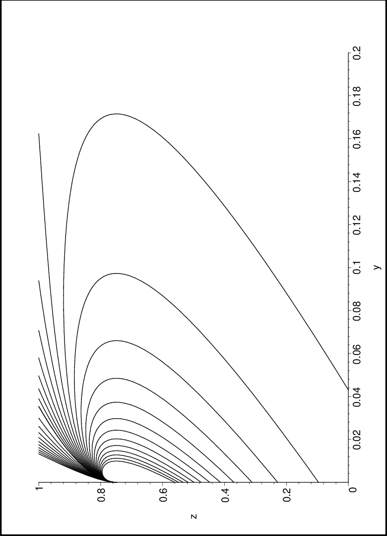
This yields the rays that emanate from (0,γ)(0,\gamma) in parametric form. Several rays are sketched in Figure 1.

Refer to caption
Figure 1: A sketch of the rays from (0,γ)(0,\gamma).

Combining the terms depending on tt we have another useful expression for y⁡(s,t)y(s,t) and z⁡(s,t)z(s,t)

y⁡(s,t)=A1​(s)Δ​(eΔ​t−1)+A2​(s)Δ​(1−e−Δ​t)+[A3​(s)−γ]​ty(s,t)=\frac{A_{1}(s)}{\Delta}\left(e^{\Delta t}-1\right)+\frac{A_{2}(s)}{\Delta}\left(1-e^{-\Delta t}\right)+\left[A_{3}(s)-\gamma\right]t (26)
z⁡(s,t)=A1​(s)​eΔ​t+A2​(s)​e−Δ​t+A3​(s)z(s,t)=A_{1}(s)e^{\Delta t}+A_{2}(s)e^{-\Delta t}+A_{3}(s) (27)

with

A1​(s)\displaystyle A_{1}(s) =14​Δ2​(λ+1−s+Δ)​(s​γ+ρ−λ+γ​Δ)\displaystyle=\frac{1}{4\Delta^{2}}\left(\lambda+1-s+\Delta\right)\left(s\gamma+\rho-\lambda+\gamma\Delta\right)
A2​(s)\displaystyle A_{2}(s) =14​Δ2​(λ+1−s−Δ)​(s​γ+ρ−λ−γ​Δ)\displaystyle=\frac{1}{4\Delta^{2}}\left(\lambda+1-s-\Delta\right)\left(s\gamma+\rho-\lambda-\gamma\Delta\right)
A3​(s)\displaystyle A_{3}(s) =1Δ2​[λ⁡(1+λ)+(γ−γ​λ−λ)​s+γ​s2].\displaystyle=\frac{1}{\Delta^{2}}\left[\lambda(1+\lambda)+\left(\gamma-\gamma\lambda-\lambda\right)s+\gamma s^{2}\right].

For t≥0t\geq 0 and each value of ss, (24) and (25) determine a ray in the (y,z)(y,z) plane, which starts from (0,γ)(0,\gamma) at t=0t=0. We discuss two particular rays which can be obtained in an explicit form. For s=0s=0 we can eliminate t\ t from (25) and obtain

t=1λ+1​ln⁡(z​λ+z−λρ),γ<z<1t=\frac{1}{\lambda+1}\ln\left(\frac{z\lambda+z-\lambda}{\rho}\right),\quad\gamma<z<1 (28)

and using (24) we get

y=Y0​(z)=z−γλ+1−ρ(λ+1)2​ln⁡(z​λ+z−λρ),s=0,γ≤z≤1.y=Y_{0}(z)=\frac{z-\gamma}{\lambda+1}-\frac{\rho}{\left(\lambda+1\right)^{2}}\ln\left(\frac{z\lambda+z-\lambda}{\rho}\right),\quad s=0,\quad\gamma\leq z\leq 1. (29)

Also, from (18) we have

u=λ​1−zz,for ​s=0,γ≤z≤1.u=\lambda\frac{1-z}{z},\quad\text{for \ }s=0,\quad\gamma\leq z\leq 1. (30)

For s>S0≡−ργ⁡(1−γ)s>S_{0}\equiv-\frac{\rho}{\gamma(1-\gamma)}, we have both y⁡(t)y(t) and z⁡(t)z(t) increasing for t>0t>0. When s=S0s=S_{0} the function uu is constant along the ray

u⁡(S0,t)≡u0=λγ​(1−γ),u(S_{0},t)\equiv u_{0}=\frac{\lambda}{\gamma}\left(1-\gamma\right),

y⁡(t)y(t) increases and z⁡(t)z(t) asymptotes γ2δ\frac{\gamma^{2}}{\delta} with

δ=(γ−1)2​λ+γ2,δ>0.\delta=(\gamma-1)^{2}\lambda+\gamma^{2},\quad\delta>0.

Eliminating tt we obtain

t=γ⁡(1−γ)δ​ln⁡[γ⁡(1−γ)​ργ2−δ​z],γ≤z<γ2δt=\frac{\gamma(1-\gamma)}{\delta}\ln\left[\frac{\gamma(1-\gamma)\rho}{\gamma^{2}-\delta z}\right],\quad\gamma\leq z<\frac{\gamma^{2}}{\delta}
y=Y1​(z)=[γ⁡(1−γ)]2​ρδ2​[γ2−δ​zγ⁡(1−γ)​ρ+ln⁡[γ⁡(1−γ)​ργ2−δ​z]−1],s=S0,γ≤z<γ2δ.y=Y_{1}(z)=\frac{\left[\gamma(1-\gamma)\right]^{2}\rho}{\delta^{2}}\left[\frac{\gamma^{2}-\delta z}{\gamma(1-\gamma)\rho}+\ln\left[\frac{\gamma(1-\gamma)\rho}{\gamma^{2}-\delta z}\right]-1\right],\quad s=S_{0},\quad\gamma\leq z<\frac{\gamma^{2}}{\delta}. (31)

For s<S0s<S_{0} the rays reach a maximum value in zz at t=Tmaxt=T_{\max}, where

Tmax=12​Δ​ln⁡(A2A1)T_{\max}=\frac{1}{2\Delta}\ln\left(\frac{A_{2}}{A_{1}}\right)

and we have

y⁡(s,Tmax)=−ρΔ2+A3−γ2​Δ​ln⁡(A2A1)y(s,T_{\max})=-\frac{\rho}{\Delta^{2}}+\frac{A_{3}-\gamma}{2\Delta}\ln\left(\frac{A_{2}}{A_{1}}\right) (32)
z⁡(s,Tmax)=2​A1​A2+A3.z(s,T_{\max})=2\sqrt{A_{1}A_{2}}+A_{3}. (33)

Inverting (33) we find that at t=Tmaxt=T_{\max}

s=z+λ⁡(1−z)±2​z​λ​(1−z)γ−z.s=\frac{z+\lambda(1-z)\pm 2\sqrt{z\lambda(1-z)}}{\gamma-z}. (34)

From (33) we see that z→γ2δz\rightarrow\frac{\gamma^{2}}{\delta} as s↑S0s\uparrow S_{0}. Therefore we must choose the (−)(-) sign in (34) and conclude that

Smax​(z)=z+λ⁡(1−z)−2​z​λ​(1−z)γ−z,γ<z<γ2δS_{\max}(z)=\frac{z+\lambda(1-z)-2\sqrt{z\lambda(1-z)}}{\gamma-z},\quad\gamma<z<\frac{\gamma^{2}}{\delta} (35)

which when used in (32) yields

y=Ymax​(z)=−ρΔ2​(Smax)+A3​(Smax)−γ2​Δ​(Smax)​ln⁡[A2​(Smax)A1​(Smax)],γ<z<γ2δ.y=Y_{\max}(z)=-\frac{\rho}{\Delta^{2}\left(S_{\max}\right)}+\frac{A_{3}\left(S_{\max}\right)-\gamma}{2\Delta\left(S_{\max}\right)}\ln\left[\frac{A_{2}\left(S_{\max}\right)}{A_{1}\left(S_{\max}\right)}\right],\quad\gamma<z<\frac{\gamma^{2}}{\delta}. (36)
Refer to caption
Figure 2: A sketch of the rays Y0​(z),Y1​(z)Y_{0}(z),Y_{1}(z) and the curve Ymax​(z)Y_{\max}(z).

This is the value of yy when zz reaches its maximum value. In Figure 2 we sketch the rays Y0​(z),Y_{0}(z), Y1​(z),Y_{1}(z), the critical curve Ymax​(z)Y_{\max}(z) and a pair of rays showing their intersection with Ymax​(z)Y_{\max}(z) at the maximum.

Solving for tt in (27) we obtain

𝕋⁡(s,z)={T+​(s,z),0<y<Ymax​(z),γ<z<1T−(s,z),{y>Ymax(z),γ<z<γ2δ}∪{y>0, 0<z<γ}\mathbb{T(}s,z)=\left\{\begin{array}[c]{l}T_{+}(s,z),\quad 0<y<Y_{\max}(z),\ \quad\gamma<z<1\\ T_{-}(s,z),\quad\left\{y>Y_{\max}(z),\ \gamma<z<\frac{\gamma^{2}}{\delta}\right\}\cup\left\{y>0,\ 0<z<\gamma\right\}\end{array}\right. (37)

with

T±​(s,z)=1Δ​ln⁡[z−A3±(z−A3)2−4​A1​A22​A1].T_{\pm}(s,z)=\frac{1}{\Delta}\ln\left[\frac{z-A_{3}\pm\sqrt{\left(z-A_{3}\right)^{2}-4A_{1}A_{2}}}{2A_{1}}\right].

Solving for uu in (18) we find that

u={U−​(s,z),0<y<Ymax​(z),γ<z<1U+(s,z),{y>Ymax(z),γ<z<γ2δ}∪{y>0, 0<z<γ}u=\left\{\begin{array}[c]{l}U_{-}(s,z),\quad 0<y<Y_{\max}(z),\ \gamma<z<1\\ U_{+}(s,z),\quad\left\{y>Y_{\max}(z),\ \gamma<z<\frac{\gamma^{2}}{\delta}\right\}\cup\left\{y>0,\ 0<z<\gamma\right\}\end{array}\right. (38)

where

U±​(s,z)\displaystyle U_{\pm}(s,z) =12​[s+1−λ+1z​(λ−γ​s)]\displaystyle=\frac{1}{2}\left[s+1-\lambda+\frac{1}{z}\left(\lambda-\gamma s\right)\right]
±12​ρ2+[2​(λ+1)​ρ+2​ϕ​s]​(z−γ)+[(λ+1)2+2​(1−λ)​s+s2]​(z−γ)2.\displaystyle\pm\frac{1}{2}\sqrt{\rho^{2}+\left[2\left(\lambda+1\right)\rho+2\phi s\right](z-\gamma)+\left[(\lambda+1)^{2}+2(1-\lambda)s+s^{2}\right](z-\gamma)^{2}}.

From (19) we see that the maximum value in yy is achieved at the same time that z=γz=\gamma, and that occurs at t=Tγt=T_{\gamma} with

Tγ=1Δ​ln⁡[ϕ​s−ρ​Δ+(λ+1)​ρϕ​s+ρ​Δ+(λ+1)​ρ],s<S0.T_{\gamma}=\frac{1}{\Delta}\ln\left[\frac{\phi s-\rho\Delta+\left(\lambda+1\right)\rho}{\phi s+\rho\Delta+\left(\lambda+1\right)\rho}\right],\quad s<S_{0}. (39)

When z=γ,y>0z=\gamma,\ y>0 we also have from (18)

u⁡(s,Tγ)=1,s<S0,u\left(s,T_{\gamma}\right)=1,\quad s<S_{0}, (40)

so that Ψz=0\Psi_{z}=0 when z=γ.z=\gamma.

Inverting the equations (24)-(25) we can write

s=S⁡(y,z),t=T⁡(y,z)s=S\left(y,z\right),\quad t=T(y,z)

and

Ψ⁡(y,z)=ψ⁡[S⁡(y,z),T⁡(y,z)],𝕂⁡(y,z)=K⁡[S⁡(y,z),T⁡(y,z)].\Psi(y,z)=\psi\left[S\left(y,z\right),T(y,z)\right],\quad\mathbb{K(}y,z\mathbb{)}=K\left[S\left(y,z\right),T(y,z)\right].

We will use this notation in the rest of the article.

3.3 The function Ψ\Psi

From (12e) we have

ψ˙=s​y˙+ln⁡(u)​z˙\dot{\psi}=s\dot{y}+\ln(u)\dot{z}

which we can integrate to get

ψ⁡(s,t)\displaystyle\psi(s,t) =ψ⁡(s,0)+s​y​(s,t)+∫0tln⁡[u⁡(s,r)]​d​zd​r​(s,r)​𝑑r\displaystyle=\psi(s,0)+sy(s,t)+{\displaystyle\int\limits_{0}^{t}}\ln\left[u(s,r)\right]\frac{dz}{dr}(s,r)dr
=ψ0​(s)+s​y+ln⁡(u)​z−ln⁡(u0)​γ−∫0tzu​𝑑u.\displaystyle=\psi_{0}(s)+sy+\ln(u)z-\ln\left(u_{0}\right)\gamma-{\displaystyle\int\limits_{0}^{t}}\frac{z}{u}du.

Using (18) and (13) we can write

∫0tzu​𝑑u\displaystyle{\displaystyle\int\limits_{0}^{t}}\frac{z}{u}du =∫0t(λ−γ​s)​u−λu⁡(u−r1)​(u−r2)​𝑑u=∫0t[1u+(λ−γ​s)​r1−λr1​(u−r1)​Δ−(λ−γ​s)​r2−λr2​(u−r2)​Δ]​𝑑u\displaystyle={\displaystyle\int\limits_{0}^{t}}\frac{(\lambda-\gamma s)u-\lambda}{u(u-r_{1})(u-r_{2})}du={\displaystyle\int\limits_{0}^{t}}\left[\frac{1}{u}+\frac{(\lambda-\gamma s)r_{1}-\lambda}{r_{1}(u-r_{1})\Delta}-\frac{(\lambda-\gamma s)r_{2}-\lambda}{r_{2}(u-r_{2})\Delta}\right]du
=ln⁡(uu0)+(λ−γ​s)​r1−λr1​Δ​ln⁡(u−r1u0−r1)−(λ−γ​s)​r2−λr2​Δ​ln⁡(u−r2u0−r2).\displaystyle=\ln\left(\frac{u}{u_{0}}\right)+\frac{(\lambda-\gamma s)r_{1}-\lambda}{r_{1}\Delta}\ln\left(\frac{u-r_{1}}{u_{0}-r_{1}}\right)-\frac{(\lambda-\gamma s)r_{2}-\lambda}{r_{2}\Delta}\ln\left(\frac{u-r_{2}}{u_{0}-r_{2}}\right).

Hence,

ψ⁡(s,t)\displaystyle\psi(s,t) =ψ0​(s)+s​y+(z−1)​ln⁡(u)+(1−γ)​ln⁡(u0)+(λ−γ​s)​r2−λr2​Δ​ln⁡(u−r2u0−r2)\displaystyle=\psi_{0}(s)+sy+(z-1)\ln(u)+(1-\gamma)\ln\left(u_{0}\right)+\frac{(\lambda-\gamma s)r_{2}-\lambda}{r_{2}\Delta}\ln\left(\frac{u-r_{2}}{u_{0}-r_{2}}\right)
−(λ−γ​s)​r1−λr1​Δ​ln⁡(u−r1u0−r1).\displaystyle-\frac{(\lambda-\gamma s)r_{1}-\lambda}{r_{1}\Delta}\ln\left(\frac{u-r_{1}}{u_{0}-r_{1}}\right). (41)

Obviously, ψ⁡(s,0)≡ψ0\psi(s,0)\equiv\psi_{0} is a constant since all rays start at the same point. We will determine ψ0\psi_{0} in section 3.

3.4 The transport equation

Re-writing the transport equation (11) as

[(1+z2​Ψz​z)​U+λ⁡(1+12​Ψz​z−z2​Ψz​z)​1U]​𝕂=(z−γ)​𝕂y+[z​U+λ⁡(z−1)​1U]​𝕂z\left[\left(1+\frac{z}{2}\Psi_{zz}\right)U+\lambda\left(1+\frac{1}{2}\Psi_{zz}-\frac{z}{2}\Psi_{zz}\right)\frac{1}{U}\right]\mathbb{K}=(z-\gamma)\mathbb{K}_{y}+\left[zU+\lambda(z-1)\frac{1}{U}\right]\mathbb{K}_{z}

and taking into consideration (19) and (17), we see that

[(1+z2​ψz​z)​u+λ⁡(1+12​ψz​z−z2​ψz​z)​1u]​K=y˙​Ky+z˙​Kz=K˙\left[\left(1+\frac{z}{2}\psi_{zz}\right)u+\lambda\left(1+\frac{1}{2}\psi_{zz}-\frac{z}{2}\psi_{zz}\right)\frac{1}{u}\right]K=\dot{y}K_{y}+\dot{z}K_{z}=\dot{K}

or

K˙K\displaystyle\frac{\dot{K}}{K} =(1+12​z​ψz​z)​u+λu​[1+12​(1−z)​ψz​z]\displaystyle=\left(1+\frac{1}{2}z\psi_{zz}\right)u+\frac{\lambda}{u}\left[1+\frac{1}{2}(1-z)\psi_{zz}\right]
=u+λu+12​[z​u+λu​(1−z)]​ψz​z\displaystyle=u+\frac{\lambda}{u}+\frac{1}{2}\left[zu+\frac{\lambda}{u}(1-z)\right]\psi_{zz}
=12​(u+λu)+12​∂∂z​[z​u−λu​(1−z)],\displaystyle=\frac{1}{2}\left(u+\frac{\lambda}{u}\right)+\frac{1}{2}\frac{\partial}{\partial z}\left[zu-\frac{\lambda}{u}(1-z)\right],

since u=exp⁡[∂ψ∂z].u=\exp\left[\frac{\partial\psi}{\partial z}\right]. But, z​u−λu​(1−z)=−z˙,zu-\frac{\lambda}{u}(1-z)=-\dot{z}, so that

K˙K\displaystyle\frac{\dot{K}}{K} =12​(u+λu)−12​∂z˙∂z\displaystyle=\frac{1}{2}\left(u+\frac{\lambda}{u}\right)-\frac{1}{2}\frac{\partial\dot{z}}{\partial z}
=12​(u+λu)−12​(z¨​∂t∂z+∂z˙∂s​∂s∂z).\displaystyle=\frac{1}{2}\left(u+\frac{\lambda}{u}\right)-\frac{1}{2}\left(\ddot{z}\frac{\partial t}{\partial z}+\frac{\partial\dot{z}}{\partial s}\frac{\partial s}{\partial z}\right).

Introducing the Jacobian of the transformation from Cartesian (y,z)(y,z) to ray (s,t)(s,t) coordinates

𝐉⁡(s,t)=∂z∂t​∂y∂s−∂z∂s​∂y∂t\mathbf{J}(s,t)=\frac{\partial z}{\partial t}\frac{\partial y}{\partial s}-\frac{\partial z}{\partial s}\frac{\partial y}{\partial t} (42)

we have

∂s∂z=−y˙𝐉=γ−z𝐉,∂t∂z=1𝐉​∂y∂s\frac{\partial s}{\partial z}=-\frac{\dot{y}}{\mathbf{J}}=\frac{\gamma-z}{\mathbf{J}},\quad\frac{\partial t}{\partial z}=\frac{1}{\mathbf{J}}\frac{\partial y}{\partial s}

and

𝐉˙=z¨​∂y∂s+z˙​∂y˙∂s−∂z˙∂s​y˙−∂z∂s​y¨=z¨​∂y∂s−∂z˙∂s​(z−γ).\mathbf{\dot{J}}=\ddot{z}\frac{\partial y}{\partial s}+\dot{z}\frac{\partial\dot{y}}{\partial s}-\frac{\partial\dot{z}}{\partial s}\dot{y}-\frac{\partial z}{\partial s}\ddot{y}=\ddot{z}\frac{\partial y}{\partial s}-\frac{\partial\dot{z}}{\partial s}(z-\gamma).

Hence,

K˙K\displaystyle\frac{\dot{K}}{K} =12​(u+λu)−12​J​[z¨​∂y∂s−∂z˙∂s​(z−γ)]\displaystyle=\frac{1}{2}\left(u+\frac{\lambda}{u}\right)-\frac{1}{2J}\left[\ddot{z}\frac{\partial y}{\partial s}-\frac{\partial\dot{z}}{\partial s}(z-\gamma)\right]
=12​(u+λu)−𝐉˙2​J=12​[λu​z−z˙z−𝐉˙𝐉]\displaystyle=\frac{1}{2}\left(u+\frac{\lambda}{u}\right)-\frac{\mathbf{\dot{J}}}{2J}=\frac{1}{2}\left[\frac{\lambda}{uz}-\frac{\dot{z}}{z}-\frac{\mathbf{\dot{J}}}{\mathbf{J}}\right]
=12​[ω˙ω−z˙z−𝐉˙𝐉]\displaystyle=\frac{1}{2}\left[\frac{\dot{\omega}}{\omega}-\frac{\dot{z}}{z}-\frac{\mathbf{\dot{J}}}{\mathbf{J}}\right]

where ω⁡(s,t)\omega(s,t) satisfies the ODE

dd​t​ln⁡(ω)=λu​z\frac{d}{dt}\ln(\omega)=\frac{\lambda}{uz}

which can be solved to give

ω⁡(s,t)=(λ−s​γ)​u−λu⁡[ρ+γ⁡(1−γ)​s].\omega(s,t)=\frac{\left(\lambda-s\gamma\right)u-\lambda}{u\left[\rho+\gamma(1-\gamma)s\right]}. (43)

We conclude that

K⁡(s,t)=K0​(s)​z−12​ω⁡(s,t)𝐉⁡(s,t),K(s,t)=K_{0}(s)z^{-\frac{1}{2}}\sqrt{\frac{\omega(s,t)}{\mathbf{J}(s,t)}}, (44)

with K0​(s)K_{0}(s) to be determined. As (y,z)→(0,γ)(y,z)\rightarrow(0,\gamma) (i.e., as OPENt→0)t\rightarrow 0) the Jacobian 𝐉⁡(s,t)→0.\mathbf{J}(s,t)\rightarrow 0. Therefore, the asymptotic expansion in (8) ceases to be valid.

So far we have determined the exponent ψ⁡(s,t)\psi(s,t) and the leading amplitude K⁡(s,t)K(s,t) except for the constant ψ0\psi_{0} in (41), the function K0​(s)K_{0}(s) in (44) and the power ν\nu in (8). In section 4 we will determine them by matching (8) to a corner layer solution valid in a neighborhood of the point (0,γ)(0,\gamma).

3.5 The rays from infinity

From (5), we have

Fk​(∞)=G⁡(∞,z)=exp⁡{1ε​[z​ln⁡(λ)−ln⁡(λ+1)]}​(ε−1z​ε−1),F_{k}(\infty)=G(\infty,z)=\exp\left\{\frac{1}{\varepsilon}\left[z\ln(\lambda)-\ln(\lambda+1)\right]\right\}\binom{\varepsilon^{-1}}{z\varepsilon^{-1}},

and by Stirling’s formula

G⁡(∞,z)∼ε​κ​(z)​exp⁡[1ε​Φ​(z)],ε→0,0<z<1G(\infty,z)\sim\sqrt{\varepsilon}\kappa(z)\exp\left[\frac{1}{\varepsilon}\Phi(z)\right],\quad\varepsilon\rightarrow 0,\quad 0<z<1 (45)

where

Φ⁡(z)=−z​ln⁡(z)−(1−z)​ln⁡(1−z)+z​ln⁡(λ)−ln⁡(λ+1)\Phi(z)=-z\ln(z)-(1-z)\ln(1-z)+z\ln(\lambda)-\ln(\lambda+1) (46)
κ⁡(z)=12​π​1z⁡(1−z).\kappa(z)=\frac{1}{\sqrt{2\pi}}\frac{1}{\sqrt{z(1-z)}}. (47)

Note that Φ⁡(z)\Phi(z) and κ⁡(z)\kappa(z) satisfy (10) and (11), respectively.

Denoting the scaled domain by

𝔇=[0,∞)×[0,1],\mathfrak{D=}[0,\infty)\times[0,1], (48)

we must determine what part of 𝔇\mathfrak{D} the rays from infinity fill. Defining p∞=∂Φ∂yp_{\infty}=\frac{\partial\Phi}{\partial y} and u∞=exp⁡(∂Φ∂z),u_{\infty}=\exp\left(\frac{\partial\Phi}{\partial z}\right), we have

p∞≡0,u∞=λ⁡(1−z)z.p_{\infty}\equiv 0,\quad u_{\infty}=\frac{\lambda\left(1-z\right)}{z}. (49)

(12) and (12b) yield the equations for the rays y∞​(t),z∞​(t)y_{\infty}(t),\ z_{\infty}(t)\

y˙∞=z∞−γ,z˙∞=(1+λ)​z∞−λ\dot{y}_{\infty}=z_{\infty}-\gamma,\quad\dot{z}_{\infty}=\left(1+\lambda\right)z_{\infty}-\lambda (50)

or, eliminating tt from the system (50) and writing y∞​(t)=Y∞​(z)y_{\infty}(t)=Y_{\infty}(z) we get

d​Y∞d​z=z−γ(1+λ)​z−λ.\frac{dY_{\infty}}{dz}=\frac{z-\gamma}{\left(1+\lambda\right)z-\lambda}. (51)

Solving (50) subject to the initial condition Y∞​(z0)=y0,Y_{\infty}(z_{0})=y_{0}, where (y0,z0)∈∂𝔇(y_{0},z_{0})\in\partial\mathfrak{D} we get

Y∞​(z)=y0+z−z0λ+1−ρ(λ+1)2​ln⁡[(λ+1)​z−λ(λ+1)​z0−λ],z0≠λλ+1Y_{\infty}(z)=y_{0}+\frac{z-z_{0}}{\lambda+1}-\frac{\rho}{\left(\lambda+1\right)^{2}}\ln\left[\frac{(\lambda+1)z-\lambda}{(\lambda+1)z_{0}-\lambda}\right],\quad z_{0}\neq\frac{\lambda}{\lambda+1} (52)

and when z0=λλ+1z_{0}=\frac{\lambda}{\lambda+1} the ray is a line parallel to the yy-axis given by

(y∞,z∞)≡(y,λλ+1),0≤y.(y_{\infty},\ z_{\infty})\equiv\left(y,\ \frac{\lambda}{\lambda+1}\right),\quad 0\leq y. (53)

We can interpret (52) as a family of rays emanating from the ”point” (∞,λλ+1)\left(\infty,\frac{\lambda}{\lambda+1}\right) and hitting the domain’s boundary ∂𝔇\partial\mathfrak{D} at the point (y0,z0).(y_{0},z_{0}). We divide the rays into five groups (see Figure 3) depending on the location of (y0,z0)(y_{0},z_{0}). The quantities inside the logarithms are all greater than one:

Refer to caption
Figure 3: A sketch of the rays from infinity.

1) y0≥0,z0=0.y_{0}\geq 0,\quad z_{0}=0.

Y∞​(z)=y0+zλ+1+ρ(λ+1)2​ln⁡[λλ−(λ+1)​z],0≤z<λλ+1.Y_{\infty}(z)=y_{0}+\frac{z}{\lambda+1}+\frac{\rho}{\left(\lambda+1\right)^{2}}\ln\left[\frac{\lambda}{\lambda-(\lambda+1)z}\right],\quad 0\leq z<\frac{\lambda}{\lambda+1}.

2) y0=0,0≤z0<λλ+1.y_{0}=0,\quad 0\leq z_{0}<\frac{\lambda}{\lambda+1}.

Y∞​(z)=z−z0λ+1+ρ(λ+1)2​ln⁡[(λ+1)​z0−λ(λ+1)​z−λ],z0≤z<λλ+1.Y_{\infty}(z)=\frac{z-z_{0}}{\lambda+1}+\frac{\rho}{\left(\lambda+1\right)^{2}}\ln\left[\frac{(\lambda+1)z_{0}-\lambda}{(\lambda+1)z-\lambda}\right],\quad z_{0}\leq z<\frac{\lambda}{\lambda+1}.

For z0=λλ+1z_{0}=\frac{\lambda}{\lambda+1} the ray becomes parallel to the yy-axis (53).

3) y0=0,λλ+1<z0<γ.y_{0}=0,\quad\frac{\lambda}{\lambda+1}<z_{0}<\gamma.

Y∞​(z)=z−z0λ+1−ρ(λ+1)2​ln⁡[(λ+1)​z0−λ(λ+1)​z−λ],λλ+1<z≤z0.Y_{\infty}(z)=\frac{z-z_{0}}{\lambda+1}-\frac{\rho}{\left(\lambda+1\right)^{2}}\ln\left[\frac{(\lambda+1)z_{0}-\lambda}{(\lambda+1)z-\lambda}\right],\quad\frac{\lambda}{\lambda+1}<z\leq z_{0}.

4) y0=0,z0=γ.y_{0}=0,\quad z_{0}=\gamma.

Y∞​(z)=z−γλ+1−ρ(λ+1)2​ln⁡[ρ(λ+1)​z−λ],λλ+1<z≤1.Y_{\infty}(z)=\frac{z-\gamma}{\lambda+1}-\frac{\rho}{\left(\lambda+1\right)^{2}}\ln\left[\frac{\rho}{(\lambda+1)z-\lambda}\right],\quad\frac{\lambda}{\lambda+1}<z\leq 1.

This critical ray is tangent to the zz-axis at z=γ.z=\gamma. The upper branch of the ray for γ≤z≤1\gamma\leq z\leq 1 is the same as the ray Y0​(z)Y_{0}(z) which emanated from (0,γ)(0,\gamma) and was defined in (29).

The part of the boundary corresponding to {0}×(γ,1]∪[0,Y0​(1))×{1}\left\{0\right\}\times(\gamma,1]\cup[0,Y_{0}(1))\times\left\{1\right\} is not reached by the rays.

5) y0>Y0​(1),z0=1.y_{0}>Y_{0}(1),\quad z_{0}=1.

Y∞​(z)=y0+z−1λ+1−ρ(λ+1)2​ln⁡[1(λ+1)​z−λ],λλ+1<z≤1.Y_{\infty}(z)=y_{0}+\frac{z-1}{\lambda+1}-\frac{\rho}{\left(\lambda+1\right)^{2}}\ln\left[\frac{1}{(\lambda+1)z-\lambda}\right],\quad\frac{\lambda}{\lambda+1}<z\leq 1.

The rays from infinity fill the region given by

R={0≤y,0≤z≤γ}∪{Y0(z)≤y,γ≤z≤1}.R=\left\{0\leq y,\quad 0\leq z\leq\gamma\right\}\cup\left\{Y_{0}(z)\leq y,\quad\gamma\leq z\leq 1\right\}. (54)

The complementary region RCR^{C}

RC={0≤y<Y0(z),γ≤z≤1},R^{C}=\left\{0\leq y<Y_{0}(z),\quad\gamma\leq z\leq 1\right\}, (55)

is a shadow of the rays from infinity. In RCR^{C}, GG is given by (8) as only the rays from (0,γ)(0,\gamma) are present. In the region RR below, both the rays coming from (0,γ)(0,\gamma) and the rays coming from infinity must be taken into account. We add (8) and (45) to represent GG in the asymptotic form

G⁡(y,z)∼ε​κ​(z)​exp⁡[1ε​Φ​(z)]+εν​exp⁡[1ε​Ψ​(y,z)]​𝕂​(y,z),(y,z)∈R.G(y,z)\sim\sqrt{\varepsilon}\kappa(z)\exp\left[\frac{1}{\varepsilon}\Phi(z)\right]+\varepsilon^{\nu}\exp\left[\frac{1}{\varepsilon}\Psi(y,z)\right]\mathbb{K}(y,z),\quad(y,z)\in R. (56)

We can show that Φ⁡(z)>Ψ⁡(y,z)\Phi(z)>\Psi(y,z) in the interior of R,R, so that G⁡(y,z)∼G⁡(∞,z).G(y,z)\sim G(\infty,z). However, in RR we can refine (56) to G⁡(y,z)−G⁡(∞,z)∼εν​exp⁡[1ε​Ψ​(y,z)]​𝕂​(y,z).G(y,z)-G(\infty,z)\sim\varepsilon^{\nu}\exp\left[\frac{1}{\varepsilon}\Psi(y,z)\right]\mathbb{K}(y,z).

4 The corner layer at (0,γ)(0,\gamma)

We determine the constant ν\nu in (8) and the function K0​(s)K_{0}(s) in (44) by considering carefully the region where the rays from (0,γ)(0,\gamma) enter the domain 𝔇\mathfrak{D} and using asymptotic matching. We introduce the stretched variables χ,l,\chi,\ l, the function G1​(l,χ)G_{1}(l,\chi) and the parameter α\alpha defined by

χ\displaystyle\chi =xε,χ≥0,Fk​(x)=G1​(k−c+α,xε)=G1​(l,χ)\displaystyle=\frac{x}{\varepsilon},\quad\chi\geq 0,\quad F_{k}(x)=G_{1}(k-c+\alpha,\frac{x}{\varepsilon})=G_{1}(l,\chi)
l\displaystyle l =k−c+α,−∞<l<∞\displaystyle=k-c+\alpha,\quad-\infty<l<\infty (57)
α\displaystyle\alpha =c−⌊c⌋,0<α<1.\displaystyle=c-\left\lfloor c\right\rfloor,\quad 0<\alpha<1.

Note that α\alpha is the fractional part of c.c. Use of (57) in (3) yields the equation

(l−α)​d​G1d​χ​ε−1=[γ​G1​(l+1,χ)+λ⁡(1−γ)​G1​(l−1,χ)−ϕ​G1​(l,χ)]​ε−1\displaystyle(l-\alpha)\frac{dG_{1}}{d\chi}\varepsilon^{-1}=\left[\gamma G_{1}\left(l+1,\chi\right)+\lambda(1-\gamma)G_{1}\left(l-1,\chi\right)-\phi G_{1}\left(l,\chi\right)\right]\varepsilon^{-1}
+λ⁡(α+1−l)​G1​(l−1,χ)+(l−α+1)​G1​(l+1,χ)+(λ−1)​(l−α)​G1​(l,χ)\displaystyle+\lambda(\alpha+1-l)G_{1}\left(l-1,\chi\right)+(l-\alpha+1)G_{1}\left(l+1,\chi\right)+\left(\lambda-1\right)(l-\alpha)G_{1}\left(l,\chi\right)

or, to leading order in ε,\varepsilon,

(l−α)​Fl(1)d​χ=γ​Fl+1(1)+λ⁡(1−γ)​Fl−1(1)−ϕ​Fl(1)(l-\alpha)\frac{F_{l}^{(1)}}{d\chi}=\gamma F_{l+1}^{(1)}+\lambda(1-\gamma)F_{l-1}^{(1)}-\phi F_{l}^{(1)} (58)

with G1​(l,χ)∼Fl(1)​(χ)G_{1}\left(l,\chi\right)\sim F_{l}^{(1)}\left(\chi\right) as ε→0\varepsilon\rightarrow 0 and ϕ=γ+λ−γ​λ\phi=\gamma+\lambda-\gamma\lambda.

Also (4) gives the boundary condition

Fl(1)​(0)=0,l≥1F_{l}^{(1)}(0)=0,\quad l\geq 1 (59)

and (45) implies that Fk​(∞)∼Fl(1)​(∞)F_{k}(\infty)\sim F_{l}^{(1)}(\infty)

Fl(1)​(∞)=ε​(u0)l−α​κ​(γ)​exp⁡[1ε​Φ​(γ)]F_{l}^{(1)}(\infty)=\sqrt{\varepsilon}\left(u_{0}\right)^{l-\alpha}\kappa(\gamma)\exp\left[\frac{1}{\varepsilon}\Phi(\gamma)\right] (60)

with u0=λγ​(1−γ).u_{0}=\frac{\lambda}{\gamma}\left(1-\gamma\right). For a fixed ll and χ→∞,\chi\rightarrow\infty, we approach the interior of R,R, where (56) applies. Note that Fl(1)​(∞)F_{l}^{(1)}(\infty) is the same as ε​κ​(z)​exp⁡[1ε​Φ​(z)]\sqrt{\varepsilon}\kappa(z)\exp\left[\frac{1}{\varepsilon}\Phi(z)\right] expanded for z→γ.z\rightarrow\gamma. Thus, (60) is the asymptotic matching condition between the corner layer and the solution in R.R. We shall examine the matching to RCR^{C} later.

Equation (58) admits the separable solutions

Fl(1)​(χ)=eθ​χ​hl​(θ)F_{l}^{(1)}(\chi)=e^{\theta\chi}h_{l}(\theta) (61)

if hl​(θ)h_{l}(\theta) satisfies the difference equation

γ​hl+1+λ⁡(1−γ)​hl−1=[(l−α)​θ+ϕ]​hl.\gamma h_{l+1}+\lambda(1-\gamma)h_{l-1}=\left[(l-\alpha)\theta+\phi\right]h_{l}.

Setting hl​(θ)=(u0)l2​Hl​(θ)h_{l}(\theta)=\left(u_{0}\right)^{\frac{l}{2}}H_{l}(\theta) we see that

Hl+1+Hl−1=2β​[(l−α)​θ+ϕ]​HlH_{l+1}+H_{l-1}=\frac{2}{\beta}\left[(l-\alpha)\theta+\phi\right]H_{l} (62)

with

β=2​λ​γ​(1−γ).\beta=2\sqrt{\lambda\gamma\left(1-\gamma\right)}. (63)

The only solutions to (62) which have acceptable behavior as l→∞l\rightarrow\infty are of the form

Hl​(θ)=Jl−α+ϕθ​(βθ)H_{l}(\theta)=J_{l-\alpha+\frac{\phi}{\theta}}\left(\frac{\beta}{\theta}\right)

where JJ is the Bessel function. If (61) is not to grow as χ→∞\chi\rightarrow\infty, we need θ≤0.\theta\leq 0. But except when vv is an integer, the Bessel function Jv​(x)J_{v}(x) is complex for negative argument. Therefore, we need

ϕθ−α=−1,−2,…\frac{\phi}{\theta}-\alpha=-1,-2,\ldots

or

θj=−ϕj+1−α<0,j≥0.\theta_{j}=-\frac{\phi}{j+1-\alpha}<0,\quad j\geq 0. (64)

It follows that the general solution to (58) takes the form

Fl(1)​(χ)=Fl(1)​(∞)+(u0)l2​∑j≥0aj​eθj​χ​Jl−α+ϕθj​(βθj)F_{l}^{(1)}(\chi)=F_{l}^{(1)}(\infty)+\left(u_{0}\right)^{\frac{l}{2}}{\displaystyle\sum\limits_{j\geq 0}}a_{j}e^{\theta_{j}\chi}J_{l-\alpha+\frac{\phi}{\theta_{j}}}\left(\frac{\beta}{\theta_{j}}\right)

or

Fl(1)​(χ)\displaystyle F_{l}^{(1)}(\chi) =ε​(u0)l−α​κ​(γ)​exp⁡[1ε​Φ​(γ)]\displaystyle=\sqrt{\varepsilon}\left(u_{0}\right)^{l-\alpha}\kappa(\gamma)\exp\left[\frac{1}{\varepsilon}\Phi(\gamma)\right] (65)
+(u0)l∑j≥0ajexp(−ϕj+1−αχ)Jl−1−j[−βϕ(j+1−α)]\displaystyle+\left(\sqrt{u_{0}}\right)^{l}{\displaystyle\sum\limits_{j\geq 0}}a_{j}\exp\left(-\frac{\phi}{j+1-\alpha}\chi\right)J_{l-1-j}\left[-\frac{\beta}{\phi}(j+1-\alpha)\right]

where the coefficients aja_{j} in the above (spectral) representation remain to be determined.

Taking the Laplace transform

F^l(1)​(ϑ)=∫0∞e−ϑ​χ​Fl(1)​(χ)​𝑑χ\hat{F}_{l}^{(1)}(\vartheta)={\displaystyle\int\limits_{0}^{\infty}}e^{-\vartheta\chi}F_{l}^{(1)}(\chi)d\chi

of (65) we obtain

F^l(1)​(ϑ)\displaystyle\hat{F}_{l}^{(1)}(\vartheta) =ε​(u0)l−α​κ​(γ)​exp⁡[1ε​Φ​(γ)]​1ϑ\displaystyle=\sqrt{\varepsilon}\left(u_{0}\right)^{l-\alpha}\kappa(\gamma)\exp\left[\frac{1}{\varepsilon}\Phi(\gamma)\right]\frac{1}{\vartheta} (66)
+(u0)l∑j≥0aj1ϑ+ϕj+1−αJj+1−l[βϕ(j+1−α)].\displaystyle+\left(\sqrt{u_{0}}\right)^{l}{\displaystyle\sum\limits_{j\geq 0}}a_{j}\frac{1}{\vartheta+\frac{\phi}{j+1-\alpha}}J_{j+1-l}\left[\frac{\beta}{\phi}(j+1-\alpha)\right].

Thus, the only singularities of F^l(1)​(ϑ)\hat{F}_{l}^{(1)}(\vartheta) are simple poles at ϑ=0\vartheta=0 and ϑ=θj,j≥0.\vartheta=\theta_{j},\quad\ j\geq 0. It is well known that the gamma function Γ⁡(z)\Gamma(z) has simple poles at z=0,−1,−2,…z=0,-1,-2,\ldots. Hence, we shall represent F^l​(ϑ)\hat{F}_{l}(\vartheta) as

F^l(1)​(ϑ)=(u0)l​1ϑ​Γ​(ϕϑ+1−α)​Jl−α+ϕϑ​(βϑ)​f​(ϑ)\hat{F}_{l}^{(1)}(\vartheta)=\left(\sqrt{u_{0}}\right)^{l}\frac{1}{\vartheta}\Gamma\left(\frac{\phi}{\vartheta}+1-\alpha\right)J_{l-\alpha+\frac{\phi}{\vartheta}}\left(\frac{\beta}{\vartheta}\right)f(\vartheta) (67)

where f⁡(ϑ)f(\vartheta) is chosen such that Γ⁡(ϕϑ+1−α)​Jl−α+ϕϑ​(βϑ)​f​(ϑ)\Gamma\left(\frac{\phi}{\vartheta}+1-\alpha\right)J_{l-\alpha+\frac{\phi}{\vartheta}}\left(\frac{\beta}{\vartheta}\right)f(\vartheta) is analytic for Re⁡(ϑ)>−ϕ1−α\operatorname{Re}(\vartheta)>-\frac{\phi}{1-\alpha}. Taking the Laplace transform in (65) we get the equation

(l−α)​ϑ​F^l(1)=γ​F^l+1(1)+λ⁡(1−γ)​F^l−1(1)−ϕ​F^l(1),l≥1(l-\alpha)\vartheta\hat{F}_{l}^{(1)}=\gamma\hat{F}_{l+1}^{(1)}+\lambda(1-\gamma)\hat{F}_{l-1}^{(1)}-\phi\hat{F}_{l}^{(1)},\ l\geq 1

which is satisfied by (67). By the inversion formula of the Laplace transform we have

Fl(1)​(χ)=(u0)l​12​π​i​∫Breχ​ϑ​1ϑ​Γ​(ϕϑ+1−α)​Jl−α+ϕϑ​(βϑ)​f​(ϑ)​𝑑ϑF_{l}^{(1)}(\chi)=\left(\sqrt{u_{0}}\right)^{l}\frac{1}{2\pi i}{\displaystyle\int\limits_{\mathrm{Br}}}e^{\chi\vartheta}\frac{1}{\vartheta}\Gamma\left(\frac{\phi}{\vartheta}+1-\alpha\right)J_{l-\alpha+\frac{\phi}{\vartheta}}\left(\frac{\beta}{\vartheta}\right)f(\vartheta)d\vartheta

where Br\mathrm{Br} is a vertical contour in the complex ϑ−\vartheta-plane on which Re⁡(ϑ)>0.\operatorname{Re}(\vartheta)>0.

Since the residue of F^l(1)​(ϑ)\hat{F}_{l}^{(1)}(\vartheta) at ϑ=0\vartheta=0 corresponds to Fl(1)​(∞)F_{l}^{(1)}(\infty), we must have

(u0)l​Γ​(ϕϑ+1−α)​Jl−α+ϕϑ​(βϑ)​f​(ϑ)→ε​(u0)l−α​κ​(γ)​exp⁡[1ε​Φ​(γ)]\left(\sqrt{u_{0}}\right)^{l}\Gamma\left(\frac{\phi}{\vartheta}+1-\alpha\right)J_{l-\alpha+\frac{\phi}{\vartheta}}\left(\frac{\beta}{\vartheta}\right)f(\vartheta)\rightarrow\sqrt{\varepsilon}\left(u_{0}\right)^{l-\alpha}\kappa(\gamma)\exp\left[\frac{1}{\varepsilon}\Phi(\gamma)\right]

as ϑ→0.\vartheta\rightarrow 0. In that limit we see that

Γ⁡(ϕϑ+1−α)​Jl−α+ϕϑ​(βϑ)∼ϑρ​(u0)ϕϑ+l−α​eρ−ϕϑ​(ϕϑ)ϕϑ+12−α,ϑ→0.\Gamma\left(\frac{\phi}{\vartheta}+1-\alpha\right)J_{l-\alpha+\frac{\phi}{\vartheta}}\left(\frac{\beta}{\vartheta}\right)\sim\sqrt{\frac{\vartheta}{\rho}}\left(\sqrt{u_{0}}\right)^{\frac{\phi}{\vartheta}+l-\alpha}e^{\frac{\rho-\phi}{\vartheta}}\left(\frac{\phi}{\vartheta}\right)^{\frac{\phi}{\vartheta}+\frac{1}{2}-\alpha},\quad\vartheta\rightarrow 0.

Therefore, we write

f⁡(ϑ)=ε​(u0)−α​ρϕ​κ​(γ)​exp⁡[1ε​Φ​(γ)+Υ⁡(ϑ)]​f~​(ϑ)f(\vartheta)=\sqrt{\varepsilon}\left(\sqrt{u_{0}}\right)^{-\alpha}\sqrt{\frac{\rho}{\phi}}\kappa(\gamma)\exp\left[\frac{1}{\varepsilon}\Phi(\gamma)+\Upsilon(\vartheta)\right]\tilde{f}(\vartheta) (68)

where

Υ⁡(ϑ)=(ϕϑ−α)​ln⁡(ϑϕ)+2​λ​(1−γ)ϑ−ϕ2​ϑ​ln⁡(u0)\Upsilon(\vartheta)=\left(\frac{\phi}{\vartheta}-\alpha\right)\ln\left(\frac{\vartheta}{\phi}\right)+\frac{2\lambda\left(1-\gamma\right)}{\vartheta}-\frac{\phi}{2\vartheta}\ln\left(u_{0}\right) (69)

and f~​(ϑ)\tilde{f}(\vartheta) is entire, with f~​(0)=1.\tilde{f}(0)=1.

By combining the preceding results we have

Fl(1)​(χ)\displaystyle F_{l}^{(1)}(\chi) =ε​ρϕ​κ​(γ)​(u0)l−α​exp⁡[1ε​Φ​(γ)]\displaystyle=\sqrt{\varepsilon}\sqrt{\frac{\rho}{\phi}}\kappa(\gamma)\left(\sqrt{u_{0}}\right)^{l-\alpha}\exp\left[\frac{1}{\varepsilon}\Phi(\gamma)\right] (70)
×12​π​i​∫B​reχ​ϑ​1ϑ​Γ​(ϕϑ+1−α)​Jl−α+ϕϑ​(βϑ)​exp⁡[Υ⁡(ϑ)]​f~​(ϑ)​𝑑ϑ.\displaystyle\times\frac{1}{2\pi i}{\displaystyle\int\limits_{Br}}e^{\chi\vartheta}\frac{1}{\vartheta}\Gamma\left(\frac{\phi}{\vartheta}+1-\alpha\right)J_{l-\alpha+\frac{\phi}{\vartheta}}\left(\frac{\beta}{\vartheta}\right)\exp\left[\Upsilon(\vartheta)\right]\tilde{f}(\vartheta)d\vartheta.

The boundary condition (59) implies that

limϑ→∞​[ϑ​F^l(1)​(ϑ)]=0,l≥1.\underset{\vartheta\rightarrow\infty}{\lim}\left[\vartheta\hat{F}_{l}^{(1)}(\vartheta)\right]=0,\quad l\geq 1.

From (70) we have

1ϑ​Γ​(ϕϑ+1−α)​Jl−α+ϕϑ​(βϑ)​exp⁡[Υ⁡(ϑ)]∼(1ϑ)l+1​Γ⁡(1−α)Γ⁡(l−α+1)​(β2)l−α​ϕα,ϑ→∞.\frac{1}{\vartheta}\Gamma\left(\frac{\phi}{\vartheta}+1-\alpha\right)J_{l-\alpha+\frac{\phi}{\vartheta}}\left(\frac{\beta}{\vartheta}\right)\exp\left[\Upsilon(\vartheta)\right]\sim\left(\frac{1}{\vartheta}\right)^{l+1}\frac{\Gamma\left(1-\alpha\right)}{\Gamma\left(l-\alpha+1\right)}\left(\frac{\beta}{2}\right)^{l-\alpha}\phi^{\alpha},\quad\vartheta\rightarrow\infty.

Fixing l=1l=1, we get f~​(ϑ)=o⁡(ϑ),ϑ→∞\tilde{f}(\vartheta)=o\left(\vartheta\right),\quad\vartheta\rightarrow\infty and by Liouville’s theorem this forces f~​(ϑ)\tilde{f}(\vartheta) to be a constant. Since f~​(0)=1,\tilde{f}(0)=1, we have f~​(ϑ)≡1.\tilde{f}(\vartheta)\equiv 1. Thus, (70) becomes

Fl(1)​(χ)\displaystyle F_{l}^{(1)}(\chi) =ε​ρϕ​κ​(γ)​(u0)l−α​exp⁡[1ε​Φ​(γ)]\displaystyle=\sqrt{\varepsilon}\sqrt{\frac{\rho}{\phi}}\kappa(\gamma)\left(\sqrt{u_{0}}\right)^{l-\alpha}\exp\left[\frac{1}{\varepsilon}\Phi(\gamma)\right] (71)
×12​π​i​∫B​reχ​ϑ​1ϑ​Γ​(ϕϑ+1−α)​Jl−α+ϕϑ​(βϑ)​exp⁡[Υ⁡(ϑ)]​𝑑ϑ.\displaystyle\times\frac{1}{2\pi i}{\displaystyle\int\limits_{Br}}e^{\chi\vartheta}\frac{1}{\vartheta}\Gamma\left(\frac{\phi}{\vartheta}+1-\alpha\right)J_{l-\alpha+\frac{\phi}{\vartheta}}\left(\frac{\beta}{\vartheta}\right)\exp\left[\Upsilon(\vartheta)\right]d\vartheta.

The coefficients aja_{j} in the spectral expansion (65) are determined from (71) by applying the residue theorem. Noting that

Res[Γ⁡(ϕϑ+1−α),ϑ=θj]=−ϕ(j+1−α)2​(−1)jj!\operatorname*{Res}\left[\Gamma\left(\frac{\phi}{\vartheta}+1-\alpha\right),\ \vartheta=\theta_{j}\right]=-\frac{\phi}{\left(j+1-\alpha\right)^{2}}\frac{\left(-1\right)^{j}}{j!}

we obtain

aj=ε​ρϕ​κ​(γ)​(u0)−α​exp⁡[1ε​Φ​(γ)+Υ⁡(θj)]​(−1)jj!​1(j+1−α),j≥0.\ a_{j}=\sqrt{\varepsilon}\sqrt{\frac{\rho}{\phi}}\kappa(\gamma)\left(\sqrt{u_{0}}\right)^{-\alpha}\exp\left[\frac{1}{\varepsilon}\Phi(\gamma)+\Upsilon(\theta_{j})\right]\frac{\left(-1\right)^{j}}{j!}\frac{1}{\left(j+1-\alpha\right)},\quad j\geq 0. (72)

This completes the determination of the spectral and integral representations of Fl(1)​(χ)F_{l}^{(1)}(\chi) and hence the leading term for Fk​(x)F_{k}(x) in the corner region.

4.1 Matching the corner and RCR^{C} regions

In this section we shall determine the constant ψ0\psi_{0} in (41), the function K0​(s)K_{0}(s) in (44) and the power ν\nu in (8). From (29) we have

Y0​(z)∼12​ρ​(z−γ)2,z→γ.Y_{0}(z)\sim\frac{1}{2\rho}(z-\gamma)^{2},\quad z\rightarrow\gamma.

If we introduce the new variable Ω\Omega defined by

Ω=2​ρ​y(z−γ)2=2​ρ​χ(l−α)2,Ω=O⁡(1)\Omega=\frac{2\rho y}{(z-\gamma)^{2}}=\frac{2\rho\chi}{(l-\alpha)^{2}},\quad\Omega=O(1) (73)

we see that the limit χ,l→∞,Ω>1,\chi,\ l\rightarrow\infty,\ \Omega>1, corresponds to the matching between the corner and RCR^{C} regions.

We set

ϑ=εΘ,η=(l−α)ϑ+ϕ=(z−γ)Θ+ϕ,η,Θ=O(1),η,Θ>0\vartheta=\varepsilon\Theta,\quad\eta=(l-\alpha)\vartheta+\phi=(z-\gamma)\Theta+\phi,\quad\eta,\Theta=O(1),\quad\eta,\Theta>0

use this in Jl−α+ϕϑ​(βϑ)J_{l-\alpha+\frac{\phi}{\vartheta}}\left(\frac{\beta}{\vartheta}\right) and let ε→0,\varepsilon\rightarrow 0, thus obtaining

Jl−α+ϕϑ​(βϑ)=Jυ​(βη​υ)∼exp⁡{υ⁡[1−(β/η)2+ln⁡(β/η1+1−(β/η)2)]}2​π​υ​1−(β/η)2J_{l-\alpha+\frac{\phi}{\vartheta}}\left(\frac{\beta}{\vartheta}\right)=J_{\upsilon}\left(\frac{\beta}{\eta}\upsilon\right)\sim\frac{\exp\left\{\upsilon\left[\sqrt{1-\left(\beta/\eta\right)^{2}}+\ln\left(\frac{\beta/\eta}{1+\sqrt{1-\left(\beta/\eta\right)^{2}}}\right)\right]\right\}}{\sqrt{2\pi\upsilon\sqrt{1-\left(\beta/\eta\right)^{2}}}}
=ε​Θ2​π​p⁡(η)​exp⁡{1ε​Θ​[p⁡(η)−η​ln⁡(η+p⁡(η)β)]}=\frac{\sqrt{\varepsilon\Theta}}{\sqrt{2\pi}\sqrt{p(\eta)}}\exp\left\{\frac{1}{\varepsilon\Theta}\left[p(\eta)-\eta\ln\left(\frac{\eta+p(\eta)}{\beta}\right)\right]\right\}

with

υ=ηε​Θ,p⁡(η)=η2−β2,p⁡(ϕ)=ρ.\upsilon=\frac{\eta}{\varepsilon\Theta},\quad p(\eta)=\sqrt{\eta^{2}-\beta^{2}},\quad p(\phi)=\rho. (74)

Use of Stirling’s formula gives

Γ⁡(ϕε​Θ+1−α)∼2​π​exp⁡{ϕε​Θ​[ln⁡(ϕε​Θ)−1]}​(ϕε​Θ)12−α\Gamma\left(\frac{\phi}{\varepsilon\Theta}+1-\alpha\right)\sim\sqrt{2\pi}\exp\left\{\frac{\phi}{\varepsilon\Theta}\left[\ln\left(\frac{\phi}{\varepsilon\Theta}\right)-1\right]\right\}\left(\frac{\phi}{\varepsilon\Theta}\right)^{\frac{1}{2}-\alpha}

and from (69) we have

exp⁡[Υ⁡(ε​Θ)]=exp⁡{1ε​Θ​[ϕ​ln⁡(ε​Θϕ)+2​λ​(1−γ)−ϕ2​ln⁡(u0)]}​(ε​Θϕ)−α.\exp\left[\Upsilon(\varepsilon\Theta)\right]=\exp\left\{\frac{1}{\varepsilon\Theta}\left[\phi\ln\left(\frac{\varepsilon\Theta}{\phi}\right)+2\lambda\left(1-\gamma\right)-\frac{\phi}{2}\ln\left(u_{0}\right)\right]\right\}\left(\frac{\varepsilon\Theta}{\phi}\right)^{-\alpha}.

Therefore,

Jυ​(βη​υ)​Γ​(ϕε​Θ+1−α)​exp⁡[Υ⁡(ε​Θ)]∼\displaystyle J_{\upsilon}\left(\frac{\beta}{\eta}\upsilon\right)\Gamma\left(\frac{\phi}{\varepsilon\Theta}+1-\alpha\right)\exp\left[\Upsilon(\varepsilon\Theta)\right]\sim (75)
ϕp⁡(η)​exp⁡{1ε​Θ​[p⁡(η)−η​ln⁡(η+p⁡(η)β)−ρ−ϕ2​ln⁡(u0)]}.\displaystyle\frac{\sqrt{\phi}}{\sqrt{p(\eta)}}\exp\left\{\frac{1}{\varepsilon\Theta}\left[p(\eta)-\eta\ln\left(\frac{\eta+p(\eta)}{\beta}\right)-\rho-\frac{\phi}{2}\ln\left(u_{0}\right)\right]\right\}.

Using (75) in (71) yields, in terms of zz and Ω,\Omega,

Fl(1)​(χ)\displaystyle F_{l}^{(1)}(\chi) ∼ε​ρ​κ​(γ)​exp⁡{1ε​[Φ⁡(γ)+z−γ2​ln⁡(u0)]}\displaystyle\sim\sqrt{\varepsilon}\sqrt{\rho}\kappa(\gamma)\exp\left\{\frac{1}{\varepsilon}\left[\Phi(\gamma)+\frac{z-\gamma}{2}\ln\left(u_{0}\right)\right]\right\} (76)
×12​π​i​∫Br′1η−ϕ​1p⁡(η)​exp⁡[1ε​(z−γ)​g​(η)]​𝑑η\displaystyle\times\frac{1}{2\pi i}{\displaystyle\int\limits_{\mathrm{Br}^{\prime}}}\frac{1}{\eta-\phi}\frac{1}{\sqrt{p(\eta)}}\exp\left[\frac{1}{\varepsilon}\left(z-\gamma\right)g(\eta)\right]d\eta

where

g⁡(η)=(η−ϕ)​Ω2​ρ+1η−ϕ​[p⁡(η)−η​ln⁡(η+p⁡(η)β)−ρ−ϕ2​ln⁡(u0)]g(\eta)=\frac{\left(\eta-\phi\right)\Omega}{2\rho}+\frac{1}{\eta-\phi}\left[p(\eta)-\eta\ln\left(\frac{\eta+p(\eta)}{\beta}\right)-\rho-\frac{\phi}{2}\ln\left(u_{0}\right)\right] (77)

and Br′\mathrm{Br}^{\prime} is a vertical contour in the complex plane with Re⁡(η)>ϕ.\operatorname{Re}(\eta)>\phi. For ε→0\varepsilon\rightarrow 0 with Ω\Omega fixed, we can evaluate (76) by the saddle point method to get

Fl(1)​(χ)∼ε​ρ​κ​(γ)​exp⁡{1ε​[Φ⁡(γ)+z−γ2​ln⁡(u0)]}\displaystyle F_{l}^{(1)}(\chi)\sim\sqrt{\varepsilon}\sqrt{\rho}\kappa(\gamma)\exp\left\{\frac{1}{\varepsilon}\left[\Phi(\gamma)+\frac{z-\gamma}{2}\ln\left(u_{0}\right)\right]\right\} (78)
×ε2​π​1z−γ​1η∗−ϕ​1p⁡(η∗)​exp⁡[1ε​(z−γ)​g​(η∗)]​1g′′​(η∗)\displaystyle\times\frac{\sqrt{\varepsilon}}{\sqrt{2\pi}}\frac{1}{\sqrt{z-\gamma}}\frac{1}{\eta^{\ast}-\phi}\frac{1}{\sqrt{p(\eta^{\ast})}}\exp\left[\frac{1}{\varepsilon}\left(z-\gamma\right)g(\eta^{\ast})\right]\frac{1}{\sqrt{g^{\prime\prime}(\eta^{\ast})}}

where the saddle point η∗​(Ω)\eta^{\ast}\left(\Omega\right) is defined by g′​(η∗)=0g^{\prime}(\eta^{\ast})=0. Note that η∗​(Ω)>ϕ\eta^{\ast}\left(\Omega\right)>\phi for Ω>1,\Omega>1, i.e., the saddle point η∗​(Ω)\eta^{\ast}\left(\Omega\right) lies to the right of the pole at η=ϕ\eta=\phi and the integrand is analytic for Re⁡(η)>ϕ\operatorname{Re}(\eta)>\phi.

Taking derivatives in (77) we find that

g′​(η)=Ω2​ρ+1(η−ϕ)2​[ρ+ϕ2​ln⁡(u0)+ϕ​ln⁡(η+p⁡(η)β)−p⁡(η)]g^{\prime}(\eta)=\frac{\Omega}{2\rho}+\frac{1}{\left(\eta-\phi\right)^{2}}\left[\rho+\frac{\phi}{2}\ln\left(u_{0}\right)+\phi\ln\left(\frac{\eta+p(\eta)}{\beta}\right)-p(\eta)\right] (79)
g′′​(η)=1(η−ϕ)3​[η2+2​η​ϕ−ϕ2−2​β2p⁡(η)−2​ϕ​ln⁡(η+p⁡(η)β)−2​ρ−ϕ​ln⁡(u0)].g^{\prime\prime}(\eta)=\frac{1}{\left(\eta-\phi\right)^{3}}\left[\frac{\eta^{2}+2\eta\phi-\phi^{2}-2\beta^{2}}{p(\eta)}-2\phi\ln\left(\frac{\eta+p(\eta)}{\beta}\right)-2\rho-\phi\ln\left(u_{0}\right)\right]. (80)

From (79) we observe that g′​(η∗)=0g^{\prime}(\eta^{\ast})=0 if η∗=ϕ\eta^{\ast}=\phi and Ω=1,\Omega=1, which implies that η∗​(1)=ϕ.\eta^{\ast}\left(1\right)=\phi. To determine η∗\eta^{\ast} for Ω∼1,\Omega\sim 1, we use (79) and an expansion of the form

η∗​(Ω)∼ϕ+a1​(Ω−1)+a2​(Ω−1)2+a3​(Ω−1)3+⋯.\eta^{\ast}\left(\Omega\right)\sim\phi+a_{1}\left(\Omega-1\right)+a_{2}\left(\Omega-1\right)^{2}+a_{3}\left(\Omega-1\right)^{3}+\cdots. (81)

Using (81) in (79) and expanding the latter in powers of Ω−1,\Omega-1, we find that

a1=−3​ρ22​ϕ,a2=−27​ρ232​ϕ3​(ρ2−3​ϕ2)a_{1}=-\frac{3\rho^{2}}{2\phi},\quad a_{2}=-\frac{27\rho^{2}}{32\phi^{3}}\left(\rho^{2}-3\phi^{2}\right)

and

g⁡(η∗)\displaystyle g(\eta^{\ast}) ∼12​ln⁡(u0)−3​ρ8​ϕ​(Ω−1)2,g′′​(η∗)∼ϕ3​ρ3,\displaystyle\sim\frac{1}{2}\ln\left(u_{0}\right)-\frac{3\rho}{8\phi}\left(\Omega-1\right)^{2},\quad g^{\prime\prime}(\eta^{\ast})\sim\frac{\phi}{3\rho^{3}},
1η∗−ϕ\displaystyle\quad\frac{1}{\eta^{\ast}-\phi} ∼−2​ϕ3​ρ2​(Ω−1)−1,1p⁡(η∗)∼1ρ\displaystyle\sim-\frac{2\phi}{3\rho^{2}}\left(\Omega-1\right)^{-1},\quad\frac{1}{\sqrt{p(\eta^{\ast})}}\sim\frac{1}{\sqrt{\rho}}

from which we conclude that as (y,z)→(0,γ)(y,z)\rightarrow(0,\gamma)

Fl(1)​(χ)∼−13​επ​ϕρ​1γ⁡(1−γ)​1z−γ​(Ω−1)−1​exp⁡{1ε​[Φ⁡(γ)+(z−γ)​ln⁡(u0)]}.F_{l}^{(1)}(\chi)\sim-\frac{1}{\sqrt{3}}\frac{\varepsilon}{\pi}\frac{\sqrt{\phi}}{\sqrt{\rho}}\frac{1}{\sqrt{\gamma\left(1-\gamma\right)}}\frac{1}{\sqrt{z-\gamma}}\left(\Omega-1\right)^{-1}\exp\left\{\frac{1}{\varepsilon}\left[\Phi(\gamma)+\left(z-\gamma\right)\ln\left(u_{0}\right)\right]\right\}. (82)

We next evaluate KK and ψ\psi in (8) near the corner (0,γ).(0,\gamma).Using T+​(s,z),T_{+}(s,z), (cf. (37)) in (24) and expanding for small ss, we obtain

y∼Y0​(z)−Y2​(z)​sy\sim Y_{0}(z)-Y_{2}(z)s (83)

with

Y2​(z)=2​ζ(λ+1)4​ln⁡(z+z​λ−λρ)\displaystyle Y_{2}(z)=\frac{2\zeta}{\left(\lambda+1\right)^{4}}\ln\left(\frac{z+z\lambda-\lambda}{\rho}\right) (84)
−z−γ(λ+1)​(λ​z+z−λ)2​[2​ζ​ρ(λ+1)2+3​ζ(λ+1)​(z−γ)+(λ−1)​(z−γ)2],\displaystyle-\frac{z-\gamma}{\left(\lambda+1\right)\left(\lambda z+z-\lambda\right)^{2}}\left[\frac{2\zeta\rho}{\left(\lambda+1\right)^{2}}+\frac{3\zeta}{\left(\lambda+1\right)}\left(z-\gamma\right)+\left(\lambda-1\right)\left(z-\gamma\right)^{2}\right],

and

ζ=2​λ−γ+(γ−1)​λ2.\zeta=2\lambda-\gamma+(\gamma-1)\lambda^{2}. (85)

When zz is close to γ,\gamma, (83) yields

y∼12​ρ​(z−γ)2−(λ+1)​ρ+ϕ​s3​ρ3​(z−γ)3,z→γy\sim\frac{1}{2\rho}\left(z-\gamma\right)^{2}-\frac{\left(\lambda+1\right)\rho+\phi s}{3\rho^{3}}\left(z-\gamma\right)^{3},\quad z\rightarrow\gamma

or, using (73),

s∼−32​ρ2ϕ​Ω−1z−γ−(λ+1)​ρϕ,z→γ.s\sim-\frac{3}{2}\frac{\rho^{2}}{\phi}\frac{\Omega-1}{z-\gamma}-\left(\lambda+1\right)\frac{\rho}{\phi},\quad z\rightarrow\gamma. (86)

Also, from (37) we have

t∼z−γρ,z→γ.t\sim\frac{z-\gamma}{\rho},\quad z\rightarrow\gamma. (87)

We expand (41) for small tt

ψ⁡(s,t)∼ψ0+ln⁡(u0)​ρ​t,t→0\psi(s,t)\sim\psi_{0}+\ln\left(u_{0}\right)\rho t,\quad t\rightarrow 0

which taking (87) into account gives

Ψ⁡(y,z)∼ψ0+(z−γ)​ln⁡(u0),z→γ\Psi(y,z)\sim\psi_{0}+\left(z-\gamma\right)\ln\left(u_{0}\right),\quad z\rightarrow\gamma

in agreement with (82) if

ψ0=Φ⁡(γ).\psi_{0}=\Phi(\gamma). (88)

From (44) we obtain

K⁡(s,t)∼K0​(s)​1γ​3(1−γ)​ϕ​ρ​t3,t→0K(s,t)\sim K_{0}(s)\frac{1}{\sqrt{\gamma}}\sqrt{\frac{3}{\left(1-\gamma\right)\phi\rho t^{3}}},\quad t\rightarrow 0

or, using (86) and (87) in the above,

𝕂⁡(y,z)∼K0​[−32​ρ2ϕ​Ω−1z−γ]​ργ​3(1−γ)​ϕ​(z−γ)3,z→γ.\mathbb{K}(y,z)\sim K_{0}\left[-\frac{3}{2}\frac{\rho^{2}}{\phi}\frac{\Omega-1}{z-\gamma}\right]\frac{\rho}{\sqrt{\gamma}}\sqrt{\frac{3}{\left(1-\gamma\right)\phi\left(z-\gamma\right)^{3}}},\quad z\rightarrow\gamma. (89)

Matching the algebraic factors in (82) and (89) yields

K0​[−32​ρ2ϕ​Ω−1z−γ]=−13​π​ϕρ32​z−γΩ−1K_{0}\left[-\frac{3}{2}\frac{\rho^{2}}{\phi}\frac{\Omega-1}{z-\gamma}\right]=-\frac{1}{3\pi}\frac{\phi}{\rho^{\frac{3}{2}}}\frac{z-\gamma}{\Omega-1}

which implies that

K0​(s)=ρ2​π​s.K_{0}(s)=\frac{\sqrt{\rho}}{2\pi s}. (90)

Finally, the exponent of ε\varepsilon in (8) is determined from (82) and turns out to be ν=1.\nu=1. This completes the determination of the asymptotic solution corresponding to rays from the point (0,γ).(0,\gamma). To summarize, we have established the following.

Result 1

The solution of (6) is asymptotically given by

G⁡(y,z)∼ε​exp⁡[1ε​Ψ​(y,z)]​𝕂​(y,z)​ in ​RCG(y,z)\sim\varepsilon\exp\left[\frac{1}{\varepsilon}\Psi(y,z)\right]\mathbb{K}(y,z)\text{ \ in }R^{C} (91)
G⁡(∞,z)−G⁡(y,z)∼−ε​exp⁡[1ε​Ψ​(y,z)]​𝕂​(y,z)​ in ​RG(\infty,z)-G(y,z)\sim-\varepsilon\exp\left[\frac{1}{\varepsilon}\Psi(y,z)\right]\mathbb{K}(y,z)\text{ \ in }R (92)

with

G⁡(∞,z)=exp⁡{1ε​[z​ln⁡(λ)−ln⁡(λ+1)]}​(ε−1z​ε−1)G(\infty,z)=\exp\left\{\frac{1}{\varepsilon}\left[z\ln(\lambda)-\ln(\lambda+1)\right]\right\}\binom{\varepsilon^{-1}}{z\varepsilon^{-1}}
R={0≤y,0≤z≤γ}∪{Y0(z)≤y,γ≤z≤1}R=\left\{0\leq y,\quad 0\leq z\leq\gamma\right\}\cup\left\{Y_{0}(z)\leq y,\quad\gamma\leq z\leq 1\right\}
Y0​(z)=z−γλ+1−ρ(λ+1)2​ln⁡[ρ(λ+1)​z−λ],γ≤z≤1Y_{0}(z)=\frac{z-\gamma}{\lambda+1}-\frac{\rho}{\left(\lambda+1\right)^{2}}\ln\left[\frac{\rho}{(\lambda+1)z-\lambda}\right],\quad\gamma\leq z\leq 1
ρ=γ​λ+γ−λ,u0=λγ​(1−γ)\rho=\gamma\lambda+\gamma-\lambda,\quad u_{0}=\frac{\lambda}{\gamma}\left(1-\gamma\right)
Ψ⁡(y,z)\displaystyle\Psi(y,z) =ψ⁡(s,t)=ln⁡[λγ⁡(λ+1)]+s​y+(z−1)​ln⁡(u)+(λ−γ​s)​r2−λr2​Δ​ln⁡(u−r2u0−r2)\displaystyle=\psi(s,t)=\ln\left[\frac{\lambda}{\gamma\left(\lambda+1\right)}\right]+sy+(z-1)\ln(u)+\frac{(\lambda-\gamma s)r_{2}-\lambda}{r_{2}\Delta}\ln\left(\frac{u-r_{2}}{u_{0}-r_{2}}\right) (93)
−(λ−γ​s)​r1−λr1​Δ​ln⁡(u−r1u0−r1)\displaystyle-\frac{(\lambda-\gamma s)r_{1}-\lambda}{r_{1}\Delta}\ln\left(\frac{u-r_{1}}{u_{0}-r_{1}}\right)
𝕂⁡(y,z)=K⁡(s,t)=ρ2​π​s​z−12​ω⁡(s,t)𝐉⁡(s,t)\mathbb{K}(y,z)=K(s,t)=\frac{\sqrt{\rho}}{2\pi s}z^{-\frac{1}{2}}\sqrt{\frac{\omega(s,t)}{\mathbf{J}(s,t)}} (94)
r1,2​(s)=12​(s+1−λ±Δ),Δ⁡(s)=(λ−s−1)2+4​λ,r_{1,2}(s)=\frac{1}{2}\left(s+1-\lambda\pm\Delta\right),\quad\Delta(s)=\sqrt{\left(\lambda-s-1\right)^{2}+4\lambda},

(y,z)(y,z) is related to (s,t)(s,t) by (24), (25) and u⁡(s,t),ω⁡(s,t),𝐉⁡(s,t)u(s,t),\ \omega(s,t),\ \mathbf{J}(s,t) are defined in (15), (43) and (42) respectively. We note that s<0s<0 in RR so that the right side of (92) is positive. This gives the leading term for the probability

Pr[X(∞)>x=yε,Z(∞)=k=zε]\Pr\left[X(\infty)>x=\frac{y}{\varepsilon},\quad Z(\infty)=k=\frac{z}{\varepsilon}\right]

that the buffer exceeds x=N​y.x=Ny.

In the corner range where (57) applies, the leading term is given by (71), or (65) and (72).

5 Transition layer

We shall find a transition layer solution near the curve y=Y0​(z)y=Y_{0}(z) defined by (29) which separates RR and RC.R^{C}. On this curve s=0,s=0, hence (94) is not valid because 𝕂⁡(y,z)\mathbb{K}(y,z) is infinite there.

We introduce the new function Lk​(x)L_{k}(x) defined by

Fk​(x)=Fk​(∞)​Lk​(x).F_{k}(x)=F_{k}(\infty)L_{k}(x).

Then (3) yields for Lk​(x)L_{k}(x) the equation

(k−c)​Lk′=[λ⁡(k−N)−k]​Lk+λ⁡(N−k)​Lk+1+k​Lk−1(k-c)L_{k}^{\prime}=\left[\lambda\left(k-N\right)-k\right]L_{k}+\lambda\left(N-k\right)L_{k+1}+kL_{k-1}

and matching to region RR forces

Lk​(∞)=1.L_{k}(\infty)=1. (95)

In terms of the variables y=ε​x,z=ε​k,y=\varepsilon x,\quad z=\varepsilon k, the function L(1)​(y,z)=L^{(1)}(y,z)= Lk​(x)L_{k}(x) and the parameters γ=ε​c,ε=1N,\gamma=\varepsilon c,\quad\varepsilon=\frac{1}{N}, we get

(z−γ)​∂L(1)∂y=(z+λ​z−λ)​∂L(1)∂z+ε2​(z−λ​z+λ)​∂2L(1)∂z2+O⁡(∂3L(1)∂z3​ε2).(z-\gamma)\frac{\partial L^{(1)}}{\partial y}=(z+\lambda z-\lambda)\frac{\partial L^{(1)}}{\partial z}+\frac{\varepsilon}{2}(z-\lambda z+\lambda)\frac{\partial^{2}L^{(1)}}{\partial z^{2}}+O\left(\frac{\partial^{3}L^{(1)}}{\partial z^{3}}\varepsilon^{2}\right).

Introducing the stretched variable Λ\Lambda defined by

y=Y0​(z)+ε​Λy=Y_{0}(z)+\sqrt{\varepsilon}\Lambda (96)

and the function L(2)​(Λ,z)=L(1)​(y,z),L^{(2)}(\Lambda,z)=L^{(1)}(y,z), we obtain for L(2)​(Λ,z)L^{(2)}(\Lambda,z) to leading order the diffusion equation

(λ−z−λ​z)​∂L(2)∂z−12​λ​z−z−λ(λ​z+z−λ)2​(z−γ)2​∂2L(2)∂Λ2=0.(\lambda-z-\lambda z)\frac{\partial L^{(2)}}{\partial z}-\frac{1}{2}\frac{\lambda z-z-\lambda}{\left(\lambda z+z-\lambda\right)^{2}}\left(z-\gamma\right)^{2}\frac{\partial^{2}L^{(2)}}{\partial\Lambda^{2}}=0. (97)

To solve (97) we assume that L(2)​(Λ,z)L^{(2)}(\Lambda,z) is a function of the similarity variable V=Λμ⁡(z),V=\frac{\Lambda}{\mu(z)}, and let 𝔏⁡(V)=L(2)​(Λ,z),\mathfrak{L}(V)=L^{(2)}(\Lambda,z), where μ⁡(z)\mu(z) is not yet determined. From (97) we get

𝔏′′𝔏′=2​Λ​μ′​(λ​z+z−λ)3(λ​z−z−λ)​(z−γ)2\frac{\mathfrak{L}^{\prime\prime}}{\mathfrak{L}^{\prime}}=2\Lambda\mu^{\prime}\frac{\left(\lambda z+z-\lambda\right)^{3}}{\left(\lambda z-z-\lambda\right)\left(z-\gamma\right)^{2}} (98)

and (95) gives

𝔏⁡(∞)=1.\mathfrak{L}(\infty)=1. (99)

We can eliminate Λ\Lambda by choosing μ\mu to satisfy the equation

2​μ​μ′​(λ​z+z−λ)3(λ​z−z−λ)​(z−γ)2=−12\mu\mu^{\prime}\frac{\left(\lambda z+z-\lambda\right)^{3}}{\left(\lambda z-z-\lambda\right)\left(z-\gamma\right)^{2}}=-1

or equivalently

d⁡(μ2)d​z=−(λ​z−z−λ)​(z−γ)2(λ​z+z−λ)3.\frac{d\left(\mu^{2}\right)}{dz}=-\frac{\left(\lambda z-z-\lambda\right)\left(z-\gamma\right)^{2}}{\left(\lambda z+z-\lambda\right)^{3}}. (100)

We choose μ⁡(γ)=0,\mu(\gamma)=0, which is necessary for matching the transition layer with the corner layer solution (71), and solve (100) to obtain

μ⁡(z)=Y2​(z)\mu(z)=\sqrt{Y_{2}(z)} (101)

where Y2​(z)Y_{2}(z) was defined in (84).

Now (98) and (99) are just

𝔏′′=−V​𝔏′,𝔏⁡(∞)=1\mathfrak{L}^{\prime\prime}=-V\mathfrak{L}^{\prime},\quad\mathfrak{L}(\infty)=1

and the solution is

𝔏⁡(V)=12​π​∫−∞Vexp⁡(−12​τ2)​𝑑τ.\mathfrak{L}(V)=\frac{1}{\sqrt{2\pi}}{\displaystyle\int\limits_{-\infty}^{V}}\exp\left(-\frac{1}{2}\tau^{2}\right)d\tau.

Thus, the transition layer solution for y−Y0​(z)=O⁡(ε)y-Y_{0}(z)=O\left(\sqrt{\varepsilon}\right) and γ<z<1\gamma<z<1 is

Fk​(x)∼F(2)​(V,z)=ε​κ​(z)​exp⁡[1ε​Φ​(z)]​12​π​∫−∞Vexp⁡(−12​τ2)​𝑑τ.F_{k}(x)\sim F^{(2)}(V,z)=\sqrt{\varepsilon}\kappa(z)\exp\left[\frac{1}{\varepsilon}\Phi(z)\right]\frac{1}{\sqrt{2\pi}}{\displaystyle\int\limits_{-\infty}^{V}}\exp\left(-\frac{1}{2}\tau^{2}\right)d\tau. (102)

5.1 Matching the transition layer and RCR^{C} solutions

We show that as (102) is expanded as V=y−Y0​(z)μ⁡(z)​ε→−∞,V=\frac{y-Y_{0}(z)}{\mu(z)\sqrt{\varepsilon}}\rightarrow-\infty, the transition layer matches to the ray expansion, corresponding to rays emanating from (0,γ).(0,\gamma). As y→Y0​(z),y\rightarrow Y_{0}(z), from (83) and (28) we have

S⁡(y,z)∼−y−Y0​(z)Y2​(z),T⁡(y,z)∼1λ+1​ln⁡(z​λ+z−λρ).S(y,z)\sim-\frac{y-Y_{0}(z)}{Y_{2}(z)},\quad T(y,z)\sim\frac{1}{\lambda+1}\ln\left(\frac{z\lambda+z-\lambda}{\rho}\right). (103)

Using (103) in (93) and (94) and expanding for y→Y0​(z),y\rightarrow Y_{0}(z), we obtain

Ψ⁡(y,z)∼Φ⁡(z)−12​[y−Y0​(z)]2Y2​(z)\Psi\left(y,z\right)\sim\Phi(z)-\frac{1}{2}\frac{\left[y-Y_{0}(z)\right]^{2}}{Y_{2}(z)} (104)
𝕂⁡(y,z)∼−12​π​Y2​(z)y−Y0​(z)​1z⁡(1−z).\mathbb{K}(y,z)\sim-\frac{1}{2\pi}\frac{\sqrt{Y_{2}(z)}}{y-Y_{0}(z)}\frac{1}{\sqrt{z(1-z)}}. (105)

From (102) we have

F(2)​(V,z)∼−ε​exp⁡[1ε​Φ​(z)]​κ⁡(z)2​π​1V​exp⁡(−12​V2),V→−∞F^{(2)}(V,z)\sim-\sqrt{\varepsilon}\exp\left[\frac{1}{\varepsilon}\Phi(z)\right]\frac{\kappa(z)}{\sqrt{2\pi}}\frac{1}{V}\exp\left(-\frac{1}{2}V^{2}\right),\quad V\rightarrow-\infty

in agreement with (104) and (105).

6 The boundary layers at z=0z=0 and z=1z=1

6.1 The boundary layer at z=0z=0

From (94) we see that K⁡(s,t)K(s,t) is singular as z→0.z\rightarrow 0. Therefore, we find a boundary layer correction near z=0.z=0. We consider solutions of (3) which have the asymptotic form

Fk​(x)−Fk​(∞)=Fk(3)​(y)−Fk​(∞)∼εν3−k​exp⁡[1ε​Ψ​(y,0)]​Kk(3)​(y).F_{k}(x)-F_{k}(\infty)=F_{k}^{(3)}(y)-F_{k}(\infty)\sim\varepsilon^{\nu_{3}-k}\exp\left[\frac{1}{\varepsilon}\Psi(y,0)\right]K_{k}^{(3)}(y). (106)

Using (106) in (3) and expanding in powers of ε\varepsilon gives to leading order

0=(k+1)​Kk+1(3)+[γ​Ψy​(y,0)−λ]​Kk(3).0=\left(k+1\right)K_{k+1}^{(3)}+\left[\gamma\Psi_{y}(y,0)-\lambda\right]K_{k}^{(3)}. (107)

Solving (107) we obtain

Kk(3)​(y)=[λ−γ​Ψy​(y,0)]k​1k!​k(3)​(y)K_{k}^{(3)}(y)=\left[\lambda-\gamma\Psi_{y}(y,0)\right]^{k}\frac{1}{k!}k^{(3)}(y) (108)

and hence

Fk(3)​(y)−Fk​(∞)∼εν0−k​exp⁡[1ε​Ψ​(y,0)]​[λ−γ​Ψy​(y,0)]k​1k!​k(3)​(y).F_{k}^{(3)}(y)-F_{k}(\infty)\sim\varepsilon^{\nu_{0}-k}\exp\left[\frac{1}{\varepsilon}\Psi(y,0)\right]\left[\lambda-\gamma\Psi_{y}(y,0)\right]^{k}\frac{1}{k!}k^{(3)}(y). (109)

Setting k=z/ε,k=z/\varepsilon, Fk(3)​(y)−Fk​(∞)=G(1)​(y,z)F_{k}^{(3)}(y)-F_{k}(\infty)=G^{(1)}(y,z) and letting k→∞,k\rightarrow\infty, we get

G(1)​(y,z)∼εν0​exp⁡{1ε​Ψ​(y,0)+1ε​z​ln⁡[λ−γ​Ψy​(y,0)z​e]}​ε2​π​1z​k(3)​(y).G^{(1)}(y,z)\sim\varepsilon^{\nu_{0}}\exp\left\{\frac{1}{\varepsilon}\Psi(y,0)+\frac{1}{\varepsilon}z\ln\left[\frac{\lambda-\gamma\Psi_{y}(y,0)}{z}e\right]\right\}\frac{\sqrt{\varepsilon}}{\sqrt{2\pi}}\frac{1}{\sqrt{z}}k^{(3)}(y). (110)

From (92) we have

G⁡(y,z)−G⁡(∞,z)∼ε2​π​ρz​1S⁡(y,0)​exp​{1ε​Ψ​(y,0)+1ε​z​ln​[λ−γ​S​(y,0)z​e]}\displaystyle G(y,z)-G(\infty,z)\sim\frac{\varepsilon}{2\pi}\frac{\sqrt{\rho}}{\sqrt{z}}\frac{1}{S(y,0)}\exp\left\{\frac{1}{\varepsilon}\Psi(y,0)+\frac{1}{\varepsilon}z\ln\left[\frac{\lambda-\gamma S(y,0)}{z}e\right]\right\} (111)
×λ−γ​S​(y,0)[γ⁡(1−γ)​S​(y,0)+ρ]​𝐉0​(y),z→0\displaystyle\times\sqrt{\frac{\lambda-\gamma S(y,0)}{\left[\gamma(1-\gamma)S(y,0)+\rho\right]\mathbf{J}_{0}(y)}},\quad z\rightarrow 0

with

S⁡(y,0)=Ψy​(y,0),𝐉0​(y)=[γ​S​(y,0)−λ]​∂y∂s​[S⁡(y,0),T⁡(y,0)]+γ​∂z∂s​[S⁡(y,0),T⁡(y,0)].S(y,0)=\Psi_{y}(y,0),\quad\mathbf{J}_{0}(y)=\left[\gamma S(y,0)-\lambda\right]\frac{\partial y}{\partial s}\left[S(y,0),T(y,0)\right]+\gamma\frac{\partial z}{\partial s}\left[S(y,0),T(y,0)\right].

Matching (110) and (111) we conclude that

ν3=12,k(3)​(y)=ρ2​π​S​(y,0)​λ−γ​S​(y,0)[γ⁡(1−γ)​S​(y,0)+ρ]​𝐉0​(y).\nu_{3}=\frac{1}{2},\quad k^{(3)}(y)=\frac{\sqrt{\rho}}{\sqrt{2\pi}S(y,0)}\sqrt{\frac{\lambda-\gamma S(y,0)}{\left[\gamma(1-\gamma)S(y,0)+\rho\right]\mathbf{J}_{0}(y)}}.

Therefore,

Fk(3)​(y)−Fk​(∞)\displaystyle F_{k}^{(3)}(y)-F_{k}(\infty) ∼ε12−k​exp⁡[1ε​Ψ​(y,0)]​[λ−γ​S​(y,0)]k​1k!\displaystyle\sim\varepsilon^{\frac{1}{2}-k}\exp\left[\frac{1}{\varepsilon}\Psi(y,0)\right]\left[\lambda-\gamma S(y,0)\right]^{k}\frac{1}{k!} (112)
×ρ2​π​S​(y,0)​λ−γ​S​(y,0)[γ⁡(1−γ)​S​(y,0)+ρ]​𝐉0​(y).\displaystyle\times\frac{\sqrt{\rho}}{\sqrt{2\pi}S(y,0)}\sqrt{\frac{\lambda-\gamma S(y,0)}{\left[\gamma(1-\gamma)S(y,0)+\rho\right]\mathbf{J}_{0}(y)}}.

We note that the the right side of (112) is negative since S⁡(y,0)<S0<0.S(y,0)<S_{0}<0.

6.2 The boundary layer at z=1,0<y<Y0​(1)z=1,\quad 0<y<Y_{0}(1)

From (94) we see that

𝕂⁡(y,z)∼ρ2​π​S​(y,1)​−[1+(1−γ)​S​(y,1)][ρ+γ⁡(1−γ)​S​(y,1)]​𝐉1​(y)​(1−z)−12,z→1\mathbb{K}(y,z)\sim\frac{\sqrt{\rho}}{2\pi S(y,1)}\sqrt{\frac{-\left[1+\left(1-\gamma\right)S(y,1)\right]}{\left[\rho+\gamma\left(1-\gamma\right)S(y,1)\right]\mathbf{J}_{1}(y)}}\left(1-z\right)^{-\frac{1}{2}},\quad z\rightarrow 1 (113)

where

𝐉1​(y)=[(1−γ)​S​(y,1)+1]​∂y∂s​[S⁡(y,1),T⁡(y,1)]−(1−γ)​∂z∂s​[S⁡(y,1),T⁡(y,1)],\mathbf{J}_{1}(y)=\left[\left(1-\gamma\right)S(y,1)+1\right]\frac{\partial y}{\partial s}\left[S(y,1),T(y,1)\right]-(1-\gamma)\frac{\partial z}{\partial s}\left[S(y,1),T(y,1)\right],

so that 𝕂⁡(y,z)\mathbb{K}(y,z) is singular when z=1.z=1. Therefore, we introduce the new variable j=N−kj=N-k and consider solutions to (3) of the form

Fk​(x)=Fj(4)​(y)∼εν4−j​exp⁡[1ε​Ψ​(y,1)]​Kj(4)​(y).F_{k}(x)=F_{j}^{\left(4\right)}(y)\sim\varepsilon^{\nu_{4}-j}\exp\left[\frac{1}{\varepsilon}\Psi(y,1)\right]K_{j}^{\left(4\right)}(y). (114)

Using (114) in (3) gives, as ε→0,\varepsilon\rightarrow 0,

[1+(1−γ)​Ψy​(y,1)]​Kj(4)−λ⁡(j+1)​Kj+1(4)=0\left[1+(1-\gamma)\Psi_{y}(y,1)\right]K_{j}^{\left(4\right)}-\lambda\left(j+1\right)K_{j+1}^{\left(4\right)}=0

which we can solve to obtain

Kj(4)​(y)=[1+(1−γ)​Ψy​(y,1)λ]j​1j!​k(4)​(y).K_{j}^{\left(4\right)}(y)=\left[\frac{1+(1-\gamma)\Psi_{y}(y,1)}{\lambda}\right]^{j}\frac{1}{j!}k^{\left(4\right)}(y).

Hence,

Fj(4)​(y)∼εν4−j​exp⁡[1ε​Ψ​(y,1)]​[1+(1−γ)​Ψy​(y,1)λ]j​1j!​k(4)​(y).F_{j}^{\left(4\right)}(y)\sim\varepsilon^{\nu_{4}-j}\exp\left[\frac{1}{\varepsilon}\Psi(y,1)\right]\left[\frac{1+(1-\gamma)\Psi_{y}(y,1)}{\lambda}\right]^{j}\frac{1}{j!}k^{\left(4\right)}(y). (115)

From (93) we have, as z→1,z\rightarrow 1,

Ψ⁡(y,z)∼Ψ⁡(y,1)+ln⁡[1+(1−γ)​S​(y,1)λ⁡(1−z)​e]​(1−z),S⁡(y,1)=Ψy​(y,1).\Psi(y,z)\sim\Psi(y,1)+\ln\left[\frac{1+(1-\gamma)S\left(y,1\right)}{\lambda\left(1-z\right)}e\right]\left(1-z\right),\quad S\left(y,1\right)=\Psi_{y}(y,1). (116)

Expanding (115) as j→∞j\rightarrow\infty using Stirling’s formula and j=1−zεj=\frac{1-z}{\varepsilon} yields

Fj(4)​(y)∼εν4​ε2​π​11−z​k(4)​(y)​exp⁡{1ε​Ψ​(y,1)+1ε​ln⁡[1+(1−γ)​Ψy​(y,1)λ⁡(1−z)​e]​(1−z)}.F_{j}^{\left(4\right)}(y)\sim\varepsilon^{\nu_{4}}\frac{\sqrt{\varepsilon}}{\sqrt{2\pi}}\frac{1}{\sqrt{1-z}}k^{\left(4\right)}(y)\exp\left\{\frac{1}{\varepsilon}\Psi(y,1)+\frac{1}{\varepsilon}\ln\left[\frac{1+(1-\gamma)\Psi_{y}(y,1)}{\lambda\left(1-z\right)}e\right]\left(1-z\right)\right\}. (117)

Matching (113) and (116) with (117) we conclude that

ν4=12,k(4)​(y)=ρ2​π​S​(y,1)​−[1+(1−γ)​S​(y,1)][ρ+γ⁡(1−γ)​S​(y,1)]​𝐉1​(y).\nu_{4}=\frac{1}{2},\quad k^{\left(4\right)}(y)=\frac{\sqrt{\rho}}{\sqrt{2\pi}S(y,1)}\sqrt{\frac{-\left[1+\left(1-\gamma\right)S(y,1)\right]}{\left[\rho+\gamma\left(1-\gamma\right)S(y,1)\right]\mathbf{J}_{1}(y)}}.

Therefore,

Fk​(x)\displaystyle F_{k}(x) =Fj(4)​(y)∼ε12−j​exp⁡[1ε​Ψ​(y,1)]​[1+(1−γ)​S​(y,1)λ]j​1j!\displaystyle=F_{j}^{\left(4\right)}(y)\sim\varepsilon^{\frac{1}{2}-j}\exp\left[\frac{1}{\varepsilon}\Psi(y,1)\right]\left[\frac{1+(1-\gamma)S(y,1)}{\lambda}\right]^{j}\frac{1}{j!} (118)
×ρ2​π​S​(y,1)​−[1+(1−γ)​S​(y,1)][ρ+γ⁡(1−γ)​S​(y,1)]​𝐉1​(y).\displaystyle\times\frac{\sqrt{\rho}}{\sqrt{2\pi}S(y,1)}\sqrt{\frac{-\left[1+\left(1-\gamma\right)S(y,1)\right]}{\left[\rho+\gamma\left(1-\gamma\right)S(y,1)\right]\mathbf{J}_{1}(y)}}.

In the range 0<y<Y0​(1),0<y<Y_{0}(1), we have S⁡(y,1)>0.S(y,1)>0.

6.3 The corner layer near (Y0​(1),1)\left(Y_{0}(1),1\right)

When

y→Y0​(1)=ρ⁡[ln⁡(ρ)−1]+1(λ+1)2y\rightarrow Y_{0}(1)=\frac{\rho\left[\ln\left(\rho\right)-1\right]+1}{\left(\lambda+1\right)^{2}}

S⁡(y,1)→0,S\left(y,1\right)\rightarrow 0, and (118) is not defined there. We consider asymptotic solutions of (3) of the form

Fk​(x)=Fj(5)​(y)∼(λ1+λ)N​Njj!​λ−j​Kj(5)​(y)F_{k}(x)=F_{j}^{\left(5\right)}(y)\sim\left(\frac{\lambda}{1+\lambda}\right)^{N}\frac{N^{j}}{j!}\lambda^{-j}K_{j}^{\left(5\right)}(y) (119)

where j=N−kj=N-k as before. Using (119) in (3) gives the following equation for Kj(5)​(y)K_{j}^{\left(5\right)}(y)

Kj(5)−Kj+1(5)=0K_{j}^{\left(5\right)}-K_{j+1}^{\left(5\right)}=0

with solution

Kj(5)​(y)=k(5)​(y).K_{j}^{\left(5\right)}(y)=k^{\left(5\right)}(y).

Hence,

Fj(5)​(y)∼(λ1+λ)N​Njj!​λ−j​k(5)​(y).F_{j}^{\left(5\right)}(y)\sim\left(\frac{\lambda}{1+\lambda}\right)^{N}\frac{N^{j}}{j!}\lambda^{-j}k^{\left(5\right)}(y). (120)

To find k(5)​(y)k^{\left(5\right)}(y) we shall match (120) with the transition layer solution (102).

As z→1,z\rightarrow 1, (102) becomes

F(2)​[V⁡(y,z),z]∼ε​κ​(z)​exp⁡[1ε​Φ​(z)]​12​π​∫−∞V⁡(y,1)exp⁡(−12​τ2)​𝑑τF^{(2)}\left[V\left(y,z\right),z\right]\sim\sqrt{\varepsilon}\kappa(z)\exp\left[\frac{1}{\varepsilon}\Phi(z)\right]\frac{1}{\sqrt{2\pi}}{\displaystyle\int\limits_{-\infty}^{V\left(y,1\right)}}\exp\left(-\frac{1}{2}\tau^{2}\right)d\tau (121)

with

V⁡(y,1)=y−Y0​(1)Y2​(1)​1ε.V\left(y,1\right)=\frac{y-Y_{0}(1)}{Y_{2}(1)}\frac{1}{\sqrt{\varepsilon}}.

From (120) we get as j=1−zε→∞j=\frac{1-z}{\varepsilon}\rightarrow\infty

Fj(5)​(y)∼ε​κ​(z)​exp⁡[1ε​Φ​(z)]​k(5)​(y).F_{j}^{\left(5\right)}(y)\sim\sqrt{\varepsilon}\kappa(z)\exp\left[\frac{1}{\varepsilon}\Phi(z)\right]k^{\left(5\right)}(y). (122)

Matching (121) and (122) gives

k(5)​(y)=12​π​∫−∞V⁡(y,1)exp⁡(−12​τ2)​𝑑τk^{\left(5\right)}(y)=\frac{1}{\sqrt{2\pi}}{\displaystyle\int\limits_{-\infty}^{V\left(y,1\right)}}\exp\left(-\frac{1}{2}\tau^{2}\right)d\tau

and we conclude that

Fj(5)​(y)∼(λ1+λ)N​(Nλ)j​1j!​12​π​∫−∞V⁡(y,1)exp⁡(−12​τ2)​𝑑τF_{j}^{\left(5\right)}(y)\sim\left(\frac{\lambda}{1+\lambda}\right)^{N}\left(\frac{N}{\lambda}\right)^{j}\frac{1}{j!}\frac{1}{\sqrt{2\pi}}{\displaystyle\int\limits_{-\infty}^{V\left(y,1\right)}}\exp\left(-\frac{1}{2}\tau^{2}\right)d\tau (123)

where

V⁡(y,1)=y−Y0​(1)ε​[(1−γ)​(ρ−4​λ+1)(λ+1)3−2​2​λ−γ+(γ−1)​λ2(λ+1)4​ln⁡(ρ)]−12.V\left(y,1\right)=\frac{y-Y_{0}(1)}{\sqrt{\varepsilon}}\left[\frac{\left(1-\gamma\right)\left(\rho-4\lambda+1\right)}{\left(\lambda+1\right)^{3}}-2\frac{2\lambda-\gamma+\left(\gamma-1\right)\lambda^{2}}{\left(\lambda+1\right)^{4}}\ln(\rho)\right]^{-\frac{1}{2}}.\quad

6.4 The boundary layer at z=1,Y0​(1)<y<∞z=1,\quad Y_{0}(1)<y<\infty

To find the solution valid in the region 1−z=O⁡(ε),Y0​(1)<y,1-z=O(\varepsilon),\quad Y_{0}(1)<y, we immediately conclude that Fk​(x)F_{k}(x) must be of the form

Fk​(x)−Fk​(∞)=Fj(6)​(y)−(λ1+λ)N​(Nj)​λ−j∼Fj(4)​(y),F_{k}(x)-F_{k}(\infty)=F_{j}^{\left(6\right)}(y)-\left(\frac{\lambda}{1+\lambda}\right)^{N}\binom{N}{j}\lambda^{-j}\sim F_{j}^{\left(4\right)}(y), (124)

where Fj(4)​(y)F_{j}^{\left(4\right)}(y) is given by (118). This solution matches to (92) and (123) as y→Y0​(1)y\rightarrow Y_{0}(1) and as j→∞,j\rightarrow\infty, respectively.

7 The boundary x=0x=0

For x=0x=0 and k≤⌊c⌋,k\leq\left\lfloor c\right\rfloor, the values of Fk​(0)F_{k}(0) can be computed from the ray expansion, since Fk​(0)−Fk​(∞)∼ε​𝕂​(0,z)​exp⁡[1ε​Ψ​(0,z)]F_{k}(0)-F_{k}(\infty)\sim\varepsilon\mathbb{K}(0,z)\exp\left[\frac{1}{\varepsilon}\Psi(0,z)\right] is well defined. For x=0x=0 and k≥⌊c⌋+1,k\geq\left\lfloor c\right\rfloor+1, we have Fk​(0)=0F_{k}(0)=0 by (4). We now examine how this boundary condition is satisfied by considering the scale x=O⁡(1)x=O(1) (OPENy=O⁡(ε))y=O(\varepsilon)) and constructing a boundary layer correction to the ray expansion. Note that this part of the boundary is in the region RC.R^{C}.

7.1 The boundary layer at x=0,γ<z<1x=0,\quad\gamma<z<1

We shall find the solution satisfying the boundary condition (7). This boundary condition must be applied on the original xx-scale. From (93) we find that Ψ⁡(y,z)=Ψ(7)​(y,z)+o⁡(y)\Psi(y,z)=\Psi^{(7)}(y,z)+o(y), as y→0,y\rightarrow 0, where

Ψ(7)​(y,z)\displaystyle\Psi^{(7)}(y,z) =(z−γ)​ln⁡[y​e(z−γ)2]+(z−1)​ln⁡(1−z)−ln⁡(λ+1)+z​ln⁡(λ)\displaystyle=\left(z-\gamma\right)\ln\left[\frac{ye}{(z-\gamma)^{2}}\right]+(z-1)\ln(1-z)-\ln\left(\lambda+1\right)+z\ln(\lambda) (125)
−γ​ln⁡(γ)+ϕ​yz−γ​ln⁡[γ​y(z−γ)2]+yz−γ​[λ⁡(1−2​γ)+(λ−1)​z].\displaystyle-\gamma\ln(\gamma)+\frac{\phi y}{z-\gamma}\ln\left[\frac{\gamma y}{\left(z-\gamma\right)^{2}}\right]+\frac{y}{z-\gamma}\left[\lambda(1-2\gamma)+(\lambda-1)z\right].

Hence, we shall consider asymptotic solutions of the form

Fk​(x)=F(7)​(x,z)∼εν7​exp⁡[1ε​Ψ(7)​(ε​x,z)]​K(7)​(x,z).F_{k}(x)=F^{(7)}(x,z)\sim\varepsilon^{\nu_{7}}\exp\left[\frac{1}{\varepsilon}\Psi^{(7)}(\varepsilon x,z)\right]K^{(7)}(x,z). (126)

Using (126) in (6) and taking into account that y=ε​xy=\varepsilon x we get, to leading order,

∂K(7)∂z+xz−γ​∂K(7)∂x+[2+z−3​γ2​(1−z)​(z−γ)]​K(7)=0.\frac{\partial K^{(7)}}{\partial z}+\frac{x}{z-\gamma}\frac{\partial K^{(7)}}{\partial x}+\left[\frac{2+z-3\gamma}{2(1-z)(z-\gamma)}\right]K^{(7)}=0. (127)

The most general solution to (127) is

K(7)​(x,z)=1x​(1−z)32​k(7)​(Ξ),Ξ=xz−γ.K^{(7)}(x,z)=\frac{1}{x}\left(1-z\right)^{\frac{3}{2}}k^{(7)}\left(\Xi\right),\quad\Xi=\frac{x}{z-\gamma}. (128)

Hence,

F(7)​(x,z)∼εν7​exp⁡[1ε​Ψ(7)​(ε​x,z)]​1x​(1−z)32​k(7)​(Ξ).F^{(7)}(x,z)\sim\varepsilon^{\nu_{7}}\exp\left[\frac{1}{\varepsilon}\Psi^{(7)}(\varepsilon x,z)\right]\frac{1}{x}\left(1-z\right)^{\frac{3}{2}}k^{(7)}\left(\Xi\right). (129)

To find k(7)​(Ξ)k^{(7)}\left(\Xi\right) and ν7\nu_{7} we will match (129) with the corner layer solution (71).

Recalling that l−α=z−γεl-\alpha=\frac{z-\gamma}{\varepsilon} and using the asymptotic formula for the Bessel functions [1],

Jν​(z)∼12​π​ν​(e​z2​ν)ν\text{$J$}_{\nu}(z)\sim\frac{1}{\sqrt{2\pi\nu}}\left(\frac{ez}{2\nu}\right)^{\nu}

we get as ε→0\varepsilon\rightarrow 0 and ϑ\vartheta fixed

Jz−γε+ϕϑ​(βϑ)∼ε2​π​1z−γ​exp⁡{(z−γε+ϕϑ)​ln⁡[β​e​ε2​ϑ​(z−γ)]−ϕϑ}.J_{\frac{z-\gamma}{\varepsilon}+\frac{\phi}{\vartheta}}\left(\frac{\beta}{\vartheta}\right)\sim\frac{\sqrt{\varepsilon}}{\sqrt{2\pi}}\frac{1}{\sqrt{z-\gamma}}\exp\left\{\left(\frac{z-\gamma}{\varepsilon}+\frac{\phi}{\vartheta}\right)\ln\left[\frac{\beta e\varepsilon}{2\vartheta\left(z-\gamma\right)}\right]-\frac{\phi}{\vartheta}\right\}. (130)

Using (130) and writing (71) in terms of x=χ​εx=\chi\varepsilon and z=γ+(l−α)​ε,z=\gamma+(l-\alpha)\varepsilon, we have

Fl(1)​(χ)∼ε2​π​ρϕ​γ​(1−γ)​(z−γ)​exp​{1ε​[γ​ln⁡(λγ)−(1−γ)​ln⁡(1−γ)−ln⁡(λ+1)]}\displaystyle F_{l}^{(1)}(\chi)\sim\frac{\varepsilon}{2\pi}\sqrt{\frac{\rho}{\phi\gamma(1-\gamma)(z-\gamma)}}\exp\left\{\frac{1}{\varepsilon}\left[\gamma\ln\left(\frac{\lambda}{\gamma}\right)-(1-\gamma)\ln(1-\gamma)-\ln(\lambda+1)\right]\right\}
×exp⁡{z−γε​ln⁡[λ⁡(1−γ)​e​ε(z−γ)]}​12​π​i​∫B​r1ϑ​Γ​(ϕϑ+1−α)​exp⁡{1ε​[x​ϑ−(z−γ)​ln⁡(ϑ)]}\displaystyle\times\exp\left\{\frac{z-\gamma}{\varepsilon}\ln\left[\frac{\lambda(1-\gamma)e\varepsilon}{\left(z-\gamma\right)}\right]\right\}\frac{1}{2\pi i}{\displaystyle\int\limits_{Br}}\frac{1}{\vartheta}\Gamma\left(\frac{\phi}{\vartheta}+1-\alpha\right)\exp\left\{\frac{1}{\varepsilon}\left[x\vartheta-\left(z-\gamma\right)\ln\left(\vartheta\right)\right]\right\} (131)
×exp⁡{ϕϑ​ln⁡[γ​εϕ⁡(z−γ)]−α​ln⁡(ϑϕ)+2​λ​(1−γ)ϑ}​d​ϑ.\displaystyle\times\exp\left\{\frac{\phi}{\vartheta}\ln\left[\frac{\gamma\varepsilon}{\phi\left(z-\gamma\right)}\right]-\alpha\ln\left(\frac{\vartheta}{\phi}\right)+\frac{2\lambda\left(1-\gamma\right)}{\vartheta}\right\}d\vartheta.

To evaluate (131) asymptotically as ε→0\varepsilon\rightarrow 0 we shall use the saddle point method. We find that the integrand has a saddle point at ϑ=1Ξ,\vartheta=\frac{1}{\Xi}, so that

Fl(1)​(χ)∼(ε2​π)32​ρϕ​γ​(1−γ)​exp​{1ε​[z​ln⁡(λ)+(z−1)​ln⁡(1−γ)−ln⁡(λ+1)−γ​ln⁡(γ)]}\displaystyle F_{l}^{(1)}(\chi)\sim\left(\frac{\varepsilon}{2\pi}\right)^{\frac{3}{2}}\sqrt{\frac{\rho}{\phi\gamma(1-\gamma)}}\exp\left\{\frac{1}{\varepsilon}\left[z\ln\left(\lambda\right)+(z-1)\ln(1-\gamma)-\ln(\lambda+1)-\gamma\ln(\gamma)\right]\right\} (132)
×exp⁡{z−γε​ln⁡[e2​ε​Ξz−γ]+ϕ​Ξ​ln⁡[γ​εϕ⁡(z−γ)]+α​ln⁡(ϕ​Ξ)+2​λ​(1−γ)​Ξ}​1x​Ξ​Γ​(ϕ​Ξ+1−α)\displaystyle\times\exp\left\{\frac{z-\gamma}{\varepsilon}\ln\left[\frac{e^{2}\varepsilon\Xi}{z-\gamma}\right]+\phi\Xi\ln\left[\frac{\gamma\varepsilon}{\phi\left(z-\gamma\right)}\right]+\alpha\ln\left(\phi\Xi\right)+2\lambda\left(1-\gamma\right)\Xi\right\}\frac{1}{x}\Xi\Gamma\left(\phi\Xi+1-\alpha\right)

Taking the limit in (129) as x→0,z→γx\rightarrow 0,\ z\rightarrow\gamma with Ξ\Xi fixed, we obtain

F(7)​(x,z)∼εν7​exp⁡{ϕ​Ξ​ln⁡[γ​ε​Ξz−γ]−ρ​Ξ}​1x​(1−γ)32​k(7)​(Ξ)\displaystyle F^{(7)}(x,z)\sim\varepsilon^{\nu_{7}}\exp\left\{\phi\Xi\ln\left[\frac{\gamma\varepsilon\Xi}{z-\gamma}\right]-\rho\Xi\right\}\frac{1}{x}\left(1-\gamma\right)^{\frac{3}{2}}k^{(7)}\left(\Xi\right) (133)
×exp⁡{z−γε​ln⁡[e2​ε​Ξz−γ]+1ε​[(z−1)​ln⁡(1−γ)−ln⁡(λ+1)+z​ln⁡(λ)−γ​ln⁡(γ)]}.\displaystyle\times\exp\left\{\frac{z-\gamma}{\varepsilon}\ln\left[\frac{e^{2}\varepsilon\Xi}{z-\gamma}\right]+\frac{1}{\varepsilon}\left[(z-1)\ln(1-\gamma)-\ln\left(\lambda+1\right)+z\ln(\lambda)-\gamma\ln(\gamma)\right]\right\}.

Matching (133) with (132) we have

k(7)​(Ξ)=(12​π)32​ρϕ​γ​Γ​(ϕ​Ξ+1−α)​Ξ(1−γ)2​exp⁡[(α−ϕ)​Ξ​ln⁡(ϕ​Ξ)+ϕ​Ξ]k^{(7)}\left(\Xi\right)=\left(\frac{1}{2\pi}\right)^{\frac{3}{2}}\sqrt{\frac{\rho}{\phi\gamma}}\Gamma\left(\phi\Xi+1-\alpha\right)\frac{\Xi}{(1-\gamma)^{2}}\exp\left[\left(\alpha-\phi\right)\Xi\ln\left(\phi\Xi\right)+\phi\Xi\right]

and ν7=32.\nu_{7}=\frac{3}{2}. Therefore, for γ<z<1,\gamma<z<1,

F(7)​(x,z)\displaystyle F^{(7)}(x,z) ∼(ε2​π)32​xz−γε+α​ρϕ​γ​(1−z)​1z−γ​(ϕz−γ)α​Γ​(ϕ​xz−γ+1−α)\displaystyle\sim\left(\frac{\varepsilon}{2\pi}\right)^{\frac{3}{2}}x^{\frac{z-\gamma}{\varepsilon}+\alpha}\sqrt{\frac{\rho}{\phi\gamma\left(1-z\right)}}\frac{1}{z-\gamma}\left(\frac{\phi}{z-\gamma}\right)^{\alpha}\Gamma\left(\frac{\phi x}{z-\gamma}+1-\alpha\right)
×exp⁡{1ε​(z−γ)​ln⁡[e​ε(z−γ)2]+1ε​[(z−1)​ln⁡(1−z)−ln⁡(λ+1)+z​ln⁡(λ)−γ​ln⁡(γ)]}\displaystyle\times\exp\left\{\frac{1}{\varepsilon}\left(z-\gamma\right)\ln\left[\frac{e\varepsilon}{(z-\gamma)^{2}}\right]+\frac{1}{\varepsilon}\left[(z-1)\ln(1-z)-\ln\left(\lambda+1\right)+z\ln(\lambda)-\gamma\ln(\gamma)\right]\right\} (134)
×exp⁡{ϕ​xz−γ​ln⁡[γ​εϕ⁡(z−γ)]+2​λ​(1−γ)​xz−γ+(λ−1)​x}\displaystyle\times\exp\left\{\frac{\phi x}{z-\gamma}\ln\left[\frac{\gamma\varepsilon}{\phi\left(z-\gamma\right)}\right]+2\lambda\left(1-\gamma\right)\frac{x}{z-\gamma}+(\lambda-1)x\right\}

Note that from (134) we have Fk​(x)=O⁡(xk−⌊c⌋),F_{k}(x)=O\left(x^{k-\left\lfloor c\right\rfloor}\right), as x→0,x\rightarrow 0, k≥⌊c⌋+1.k\geq\left\lfloor c\right\rfloor+1.

7.2 Matching the boundary layer at x=0,γ<z<1x=0,\quad\gamma<z<1 and the RCR^{C} solution

Writing x=yε,x=\frac{y}{\varepsilon}, and using Stirling’s formula we have, as ε→0\varepsilon\rightarrow 0

Γ⁡[ϕ​y(z−γ)​ε+1−α]∼2​πε​[ϕ​y(z−γ)​ε]−α​ϕ​y(z−γ)\displaystyle\Gamma\left[\frac{\phi y}{\left(z-\gamma\right)\varepsilon}+1-\alpha\right]\sim\frac{\sqrt{2\pi}}{\sqrt{\varepsilon}}\left[\frac{\phi y}{\left(z-\gamma\right)\varepsilon}\right]^{-\alpha}\sqrt{\frac{\phi y}{\left(z-\gamma\right)}}
×exp⁡{ϕ​yε⁡(z−γ)​ln⁡[ϕ​ye⁡(z−γ)​ε]}.\displaystyle\times\exp\left\{\frac{\phi y}{\varepsilon\left(z-\gamma\right)}\ln\left[\frac{\phi y}{e\left(z-\gamma\right)\varepsilon}\right]\right\}.

Hence, (134) becomes, for x=yε→∞x=\frac{y}{\varepsilon}\rightarrow\infty

F(7)​(x,z)\displaystyle F^{(7)}(x,z) ∼ε2​π​ργ⁡(1−z)​1(z−γ)32​y\displaystyle\sim\frac{\varepsilon}{2\pi}\sqrt{\frac{\rho}{\gamma\left(1-z\right)}}\frac{1}{\left(z-\gamma\right)^{\frac{3}{2}}}\sqrt{y}
×exp⁡{1ε​(z−γ)​ln⁡[y​e(z−γ)2]+1ε​[(z−1)​ln⁡(1−z)−ln⁡(λ+1)+z​ln⁡(λ)−γ​ln⁡(γ)]}\displaystyle\times\exp\left\{\frac{1}{\varepsilon}\left(z-\gamma\right)\ln\left[\frac{ye}{(z-\gamma)^{2}}\right]+\frac{1}{\varepsilon}\left[(z-1)\ln(1-z)-\ln\left(\lambda+1\right)+z\ln(\lambda)-\gamma\ln(\gamma)\right]\right\} (135)
×exp⁡{ϕ​yε⁡(z−γ)​ln⁡[γ​y(z−γ)2]+yε​[λ−1−ρz−γ]}.\displaystyle\times\exp\left\{\frac{\phi y}{\varepsilon\left(z-\gamma\right)}\ln\left[\frac{\gamma y}{\left(z-\gamma\right)^{2}}\right]+\frac{y}{\varepsilon}\left[\lambda-1-\frac{\rho}{z-\gamma}\right]\right\}.

From (24) and (25) we get, as y→0y\rightarrow 0

s∼z−γy+ϕ​yz−γ​ln⁡[γ​y(z−γ)2]+1z−γ​[λ⁡(2−3​γ)+γ+(λ−1)​z].s\sim\frac{z-\gamma}{y}+\frac{\phi y}{z-\gamma}\ln\left[\frac{\gamma y}{\left(z-\gamma\right)^{2}}\right]+\frac{1}{z-\gamma}\left[\lambda(2-3\gamma)+\gamma+(\lambda-1)z\right]. (136)

Using (136) in (93) and (94) we find that

K⁡(s,t)∼12​π​ργ⁡(1−z)​y​(z−γ)−32,ψ⁡(s,t)∼Ψ(7)​(y,z)K(s,t)\sim\frac{1}{2\pi}\sqrt{\frac{\rho}{\gamma\left(1-z\right)}}\sqrt{y}\left(z-\gamma\right)^{-\frac{3}{2}},\quad\psi(s,t)\sim\Psi^{(7)}(y,z)

in perfect agreement with (135).

7.3 The corner layer at (0,1)(0,1)

For (y,z)(y,z) close to (0,1),(0,1), we use the variables x=yεx=\frac{y}{\varepsilon} and j=N−k,j=N-k, and look for asymptotic solutions of the form

Fk​(x)=Fj(8)​(x)∼εν8−2​j​exp⁡[1ε​Ψ(8)​(x,ε)]​Kj(8)​(x)F_{k}(x)=F_{j}^{(8)}(x)\sim\varepsilon^{\nu_{8}-2j}\exp\left[\frac{1}{\varepsilon}\Psi^{(8)}(x;\varepsilon)\right]K_{j}^{(8)}(x) (137)

with

Ψ(8)​(x,ε)=(1−γ)​ln⁡[x​ε​e(1−γ)2]−ln⁡(λ+1)+ln⁡(λ)−γ​ln⁡(γ).\Psi^{(8)}(x;\varepsilon)=\left(1-\gamma\right)\ln\left[\frac{x\varepsilon e}{(1-\gamma)^{2}}\right]-\ln\left(\lambda+1\right)+\ln(\lambda)-\gamma\ln(\gamma).

Using (137) in (3) gives, to leading order,

x​λ​(j+1)​Kj+1(8)=(1−γ)2​Kj(8)x\lambda(j+1)K_{j+1}^{\left(8\right)}=(1-\gamma)^{2}K_{j}^{\left(8\right)}

whose solution is

Kj(8)​(x)=[(1−γ)2λ​x]j​1j!​k(8)​(x).K_{j}^{\left(8\right)}(x)=\left[\frac{\left(1-\gamma\right)^{2}}{\lambda x}\right]^{j}\frac{1}{j!}k^{\left(8\right)}\left(x\right).

Hence,

Fj(8)​(x)∼exp⁡[1ε​Ψ(8)​(x,ε)]​εν8−2​j​[(1−γ)2λ​x]j​1j!​k(8)​(x).F_{j}^{(8)}(x)\sim\exp\left[\frac{1}{\varepsilon}\Psi^{(8)}(x;\varepsilon)\right]\varepsilon^{\nu_{8}-2j}\left[\frac{\left(1-\gamma\right)^{2}}{\lambda x}\right]^{j}\frac{1}{j!}k^{\left(8\right)}\left(x\right). (138)

As j→∞j\rightarrow\infty (138) gives, by Stirling’s formula,

Fj(8)​(x)∼Fj(8)​(x)∼12​π​j​exp⁡[1ε​Ψ(8)​(x,ε)+j]​εν8−2​j​[(1−γ)2λ​x​j]j​1j!​k(8)​(x).F_{j}^{(8)}(x)\sim F_{j}^{(8)}(x)\sim\frac{1}{\sqrt{2\pi j}}\exp\left[\frac{1}{\varepsilon}\Psi^{(8)}(x;\varepsilon)+j\right]\varepsilon^{\nu_{8}-2j}\left[\frac{\left(1-\gamma\right)^{2}}{\lambda xj}\right]^{j}\frac{1}{j!}k^{\left(8\right)}\left(x\right). (139)

We determine k(8)​(x)k^{\left(8\right)}\left(x\right) by matching (139) to the boundary layer expansion in (134).

Writing z=1−j​εz=1-j\varepsilon and letting z→1,z\rightarrow 1, we obtain from (134)

F(7)​(x,z)∼ε​(12​π)32​Γ​(ϕ​x1−γ+1−α)​(ϕ​x1−γ)α​ρϕ​γ​j​11−γ​ε−2​j​[(1−γ)2λ​x​j]j\displaystyle F^{(7)}(x,z)\sim\varepsilon\left(\frac{1}{2\pi}\right)^{\frac{3}{2}}\Gamma\left(\frac{\phi x}{1-\gamma}+1-\alpha\right)\left(\frac{\phi x}{1-\gamma}\right)^{\alpha}\sqrt{\frac{\rho}{\phi\gamma j}}\frac{1}{1-\gamma}\varepsilon^{-2j}\left[\frac{\left(1-\gamma\right)^{2}}{\lambda xj}\right]^{j} (140)
×exp⁡{1ε​Ψ(8)​(x,ε)+ϕ​x1−γ​ln⁡[ε​γϕ⁡(1−γ)]+x⁡(3​λ−1)}.\displaystyle\times\exp\left\{\frac{1}{\varepsilon}\Psi^{(8)}(x;\varepsilon)+\frac{\phi x}{1-\gamma}\ln\left[\frac{\varepsilon\gamma}{\phi\left(1-\gamma\right)}\right]+x(3\lambda-1)\right\}.

By comparing (139) and (140) we find that

k(8)​(x)=12​π​Γ​(ϕ​x1−γ+1−α)​(ϕ​x1−γ)α​ρϕ​γ​11−γ​exp⁡{ϕ​x1−γ​ln⁡[ε​γϕ⁡(1−γ)]+x⁡(3​λ−1)}k^{\left(8\right)}\left(x\right)=\frac{1}{2\pi}\Gamma\left(\frac{\phi x}{1-\gamma}+1-\alpha\right)\left(\frac{\phi x}{1-\gamma}\right)^{\alpha}\sqrt{\frac{\rho}{\phi\gamma}}\frac{1}{1-\gamma}\exp\left\{\frac{\phi x}{1-\gamma}\ln\left[\frac{\varepsilon\gamma}{\phi\left(1-\gamma\right)}\right]+x(3\lambda-1)\right\}

and ν8=1.\nu_{8}=1.Therefore,

Fj(8)​(x)\displaystyle F_{j}^{(8)}(x) ∼ε2​π​exp⁡{1ε​Ψ(8)​(x,ε)+ϕ​x1−γ​ln⁡[γ​ε(1−γ)​ϕ]+(3​λ−1)​x}​[(1−γ)2λ​x]j​1j!\displaystyle\sim\frac{\varepsilon}{2\pi}\exp\left\{\frac{1}{\varepsilon}\Psi^{(8)}(x;\varepsilon)+\frac{\phi x}{1-\gamma}\ln\left[\frac{\gamma\varepsilon}{\left(1-\gamma\right)\phi}\right]+(3\lambda-1)x\right\}\left[\frac{\left(1-\gamma\right)^{2}}{\lambda x}\right]^{j}\frac{1}{j!}
×Γ⁡(ϕ​x1−γ+1−α)​(ϕ​x1−γ)α​ρϕ​γ​11−γ​ε−2​j.\displaystyle\times\Gamma\left(\frac{\phi x}{1-\gamma}+1-\alpha\right)\left(\frac{\phi x}{1-\gamma}\right)^{\alpha}\sqrt{\frac{\rho}{\phi\gamma}}\frac{1}{1-\gamma}\varepsilon^{-2j}.

We can also show that the above, when expanded for x→∞,x\rightarrow\infty, matches to the boundary layer expansion in (118), valid for j=O⁡(1)j=O(1) and 0<y<Y0​(1).0<y<Y_{0}(1).

8 The marginal distribution

We will now find the equilibrium probability that the buffer content exceeds xx

Pr[X(∞)>x]=M(x)=1−∑k=0NFk(x)\Pr\left[X(\infty)>x\right]=M(x)=1-{\displaystyle\sum\limits_{k=0}^{N}}F_{k}(x) (141)

for various ranges of x.x. We will compare our results with those obtained previously by Morrison [31].

8.1 Approximation for x=O⁡(ε)=O⁡(1/N)x=O(\varepsilon)=O(1/N)

In this region we shall use the spectral representation of the corner layer solution (65), which applies for x=ε​χ=O⁡(ε)x=\varepsilon\chi=O(\varepsilon). Using the generating function

∑j=−∞∞Jj​(x)​zj=exp⁡[x2​(z−1z)]{\displaystyle\sum\limits_{j=-\infty}^{\infty}}J_{j}(x)z^{j}=\exp\left[\frac{x}{2}\left(z-\frac{1}{z}\right)\right]

we obtain

exp⁡[ρϕ​(j+1−α)]=(u0)−(j+1)​∑l=−∞∞Jl−(j+1)​[−βϕ​(j+1−α)]​(u0)l.\exp\left[\frac{\rho}{\phi}(j+1-\alpha)\right]=\left(\sqrt{u_{0}}\right)^{-(j+1)}{\displaystyle\sum\limits_{l=-\infty}^{\infty}}J_{l-(j+1)}\left[-\frac{\beta}{\phi}(j+1-\alpha)\right]\left(\sqrt{u_{0}}\right)^{l}.

Therefore,

M⁡(x)\displaystyle M(x) =M(1)​(χ)∼∑j≥0aj​exp⁡(−ϕj+1−α​χ)​exp​[ρϕ​(j+1−α)]​(u0)j+1\displaystyle=M^{(1)}(\chi)\sim{\displaystyle\sum\limits_{j\geq 0}}a_{j}\exp\left(-\frac{\phi}{j+1-\alpha}\chi\right)\exp\left[\frac{\rho}{\phi}(j+1-\alpha)\right]\left(\sqrt{u_{0}}\right)^{j+1}
=\displaystyle= ε​ρϕ​κ​(γ)​exp⁡[1ε​Φ​(γ)]​∑j≥0(−1)jj!​1(j+1−α)\displaystyle\sqrt{\varepsilon}\sqrt{\frac{\rho}{\phi}}\kappa(\gamma)\exp\left[\frac{1}{\varepsilon}\Phi(\gamma)\right]{\displaystyle\sum\limits_{j\geq 0}}\frac{\left(-1\right)^{j}}{j!}\frac{1}{\left(j+1-\alpha\right)}
×exp⁡(−ϕj+1−α​χ)​exp​[ρϕ​(j+1−α)+Υ⁡(θj)]​(u0)j+1−α.\displaystyle\times\exp\left(-\frac{\phi}{j+1-\alpha}\chi\right)\exp\left[\frac{\rho}{\phi}(j+1-\alpha)+\Upsilon(\theta_{j})\right]\left(\sqrt{u_{0}}\right)^{j+1-\alpha}.

From (69) we have

exp⁡[Υ⁡(ϑj)]=[−(j+1−α)]j+1​exp⁡[−2​λ​(1−γ)ϕ​(j+1−α)]​(u0)j+1−α.\exp\left[\Upsilon(\vartheta_{j})\right]=\left[-\left(j+1-\alpha\right)\right]^{j+1}\exp\left[-\frac{2\lambda\left(1-\gamma\right)}{\phi}(j+1-\alpha)\right]\left(\sqrt{u_{0}}\right)^{j+1-\alpha}.

Hence,

M(1)​(χ)\displaystyle M^{(1)}(\chi) ∼ε​ρϕ​κ​(γ)​exp⁡[1ε​Φ​(γ)]\displaystyle\sim\sqrt{\varepsilon}\sqrt{\frac{\rho}{\phi}}\kappa(\gamma)\exp\left[\frac{1}{\varepsilon}\Phi(\gamma)\right] (142)
×∑j≥0(j+1−α)jj!​exp⁡(−ϕj+1−α​χ)​exp​[(2​ρϕ−1)​(j+1−α)]​(u0)j+1−α.\displaystyle\times{\displaystyle\sum\limits_{j\geq 0}}\frac{\left(j+1-\alpha\right)^{j}}{j!}\exp\left(-\frac{\phi}{j+1-\alpha}\chi\right)\exp\left[\left(\frac{2\rho}{\phi}-1\right)(j+1-\alpha)\right]\left(u_{0}\right)^{j+1-\alpha}.

The formula (142) agrees with Morrison’s result (4.14) in [31], taking into account the following notational equivalences

Morrison Dominici-Knessl μ\mu 1−α1-\alpha rr ργ⁡(1−γ)=−S0\frac{\rho}{\gamma\left(1-\gamma\right)}=-S_{0} κ⁡(γ)\kappa\left(\gamma\right) −Φ⁡(γ)-\Phi(\gamma) f⁡(γ)f\left(\gamma\right) −ln⁡(u0)−2​ρϕ.-\ln\left(u_{0}\right)-2\frac{\rho}{\phi}.

8.2 Approximation for x=O⁡(ε−1)=O⁡(N)x=O(\varepsilon^{-1})=O(N)

We shall now use the asymptotic solution in the region R,R, as given by (92). We have

M(x)=M(2)(y)=−∑k=0NG(y,kN)∼−∫01exp[1εΨ(y,z)]𝕂(y,z)dzM(x)=M^{(2)}(y)=-{\displaystyle\sum\limits_{k=0}^{N}}G\left(y,\frac{k}{N}\right)\sim-{\displaystyle\int\limits_{0}^{1}}\exp\left[\frac{1}{\varepsilon}\Psi(y,z)\right]\mathbb{K(}y,z)dz

and using the saddle point method we get

M(2)​(y)∼−ε​2​π−Ψz​z​(y,γ)​exp⁡[1ε​Ψ​(y,γ)]​𝕂​(y,γ).M^{(2)}(y)\sim-\sqrt{\varepsilon}\frac{\sqrt{2\pi}}{\sqrt{-\Psi_{zz}(y,\gamma)}}\exp\left[\frac{1}{\varepsilon}\Psi(y,\gamma)\right]\mathbb{K(}y,\gamma).

We recall that for a fixed yy, Ψ⁡(y,z)\Psi(y,z) is maximal at z=γ.z=\gamma. From (38) and (39) we get

Ψz​z​(y,γ)=1ρ​S​(y,γ),𝕂⁡(y,γ)=12​π​S​(y,γ)​S⁡(y,γ)−ys​(s,Tγ)​[γ⁡(γ−1)​S​(y,γ)−ρ]\Psi_{zz}(y,\gamma)=\frac{1}{\rho}S(y,\gamma),\quad\mathbb{K(}y,\gamma)=\frac{1}{2\pi S(y,\gamma)}\sqrt{\frac{S(y,\gamma)}{-y_{s}\left(s,T_{\gamma}\right)\left[\gamma\left(\gamma-1\right)S(y,\gamma)-\rho\right]}}

where ys​(s,Tγ)y_{s}\left(s,T_{\gamma}\right) is understood to be evaluated at s=S⁡(y,γ)<S0<0.s=S(y,\gamma)<S_{0}<0. Thus,

M(2)​(y)∼−ε2​π​1S⁡(y,γ)​−S0ys​(s,Tγ)​[S0−S⁡(y,γ)]​exp⁡[1ε​Ψ​(y,γ)].M^{(2)}(y)\sim-\frac{\sqrt{\varepsilon}}{\sqrt{2\pi}}\frac{1}{S(y,\gamma)}\sqrt{\frac{-S_{0}}{y_{s}\left(s,T_{\gamma}\right)\left[S_{0}-S(y,\gamma)\right]}}\exp\left[\frac{1}{\varepsilon}\Psi(y,\gamma)\right]. (143)

From (24) and (39) we get

y⁡(s,Tγ)=−[ϕ​s+ρ⁡(λ+1)]​Tγ+2​ρΔ2y\left(s,T_{\gamma}\right)=-\frac{\left[\phi s+\rho(\lambda+1)\right]T_{\gamma}+2\rho}{\Delta^{2}}

and from (93) and (39) we have

ψ⁡(s,Tγ)=s​y​(s,Tγ)−ln⁡(λ+1)+12​[(2​γ−1)​s−(λ+1)]​Tγ+12​ln⁡[λ​sρ+s​γ​(1−γ)].\psi(s,T_{\gamma})=sy\left(s,T_{\gamma}\right)-\ln(\lambda+1)+\frac{1}{2}\left[\left(2\gamma-1\right)s-(\lambda+1)\right]T_{\gamma}+\frac{1}{2}\ln\left[\frac{\lambda s}{\rho+s\gamma(1-\gamma)}\right].

The results above agree with Morrison’s (5.15) in [31] if we reconcile notation as below

Morrison Dominici-Knessl τ\tau −s-s Z⁡(τ)Z(\tau) y⁡(s,Tγ)y\left(s,T_{\gamma}\right) ln⁡[Y⁡(σ)]\ln\left[Y(\sigma)\right] Δ⁡(−s)​Tγ​(−s)\Delta(-s)T_{\gamma}(-s) U⁡(τ)U\left(\tau\right) s​y​(s,Tγ)−ψ⁡(s,Tγ).sy\left(s,T_{\gamma}\right)-\psi(s,T_{\gamma}).

9 Summary and discussion

In most of the strip 𝔇={(y,z):y≥0, 0≤z≤1},\mathfrak{D=}\left\{(y,z):y\geq 0,\ 0\leq z\leq 1\right\}, the asymptotic expansion of Fk​(x)=G​(y,z)F_{k}(x)=G(y,z) is given by

G⁡(y,z)∼ε​exp⁡[1ε​Ψ​(y,z)]​𝕂​(y,z)​ in ​RCG(y,z)\sim\varepsilon\exp\left[\frac{1}{\varepsilon}\Psi(y,z)\right]\mathbb{K}(y,z)\text{ \ in }R^{C} (144)

or

G⁡(∞,z)−G⁡(y,z)∼−ε​exp⁡[1ε​Ψ​(y,z)]​𝕂​(y,z)​ in ​R.G(\infty,z)-G(y,z)\sim-\varepsilon\exp\left[\frac{1}{\varepsilon}\Psi(y,z)\right]\mathbb{K}(y,z)\text{ \ in }R. (145)

If we consider the continuous part of the density, given by

fk​(x)=Fk′​(x)=ε​∂G∂y​(y,z),x>0,f_{k}(x)=F_{k}^{\prime}(x)=\varepsilon\frac{\partial G}{\partial y}(y,z),\quad x>0,

the transition between RR and RCR^{C} disappears, and we have

fk​(x)∼ε​Ψy​(y,z)​exp⁡[1ε​Ψ​(y,z)]​𝕂​(y,z)=ε​exp⁡[1ε​ψ​(s,t)]​s​K​(s,t),f_{k}(x)\sim\varepsilon\Psi_{y}(y,z)\exp\left[\frac{1}{\varepsilon}\Psi(y,z)\right]\mathbb{K}(y,z)=\varepsilon\exp\left[\frac{1}{\varepsilon}\psi(s,t)\right]sK(s,t),

everywhere in the interior of𝔇.\ \mathfrak{D.} Note that 𝕂⁡(y,z)\mathbb{K}(y,z) becomes infinite along y=Y0​(z)y=Y_{0}(z) (i.e., OPENs=0),s=0), but the product Ψy​(y,z)​𝕂​(y,z)\Psi_{y}(y,z)\mathbb{K}(y,z) remains finite.

The asymptotic expansion of the boundary probabilities Fk​(0),F_{k}(0), k≤⌊c⌋k\leq\left\lfloor c\right\rfloor can be obtained by setting y=0y=0 in (145). This expression can be used to estimate the difference

Fk(∞)−Fk(0)=Pr[X(∞)>0,Z(∞)=k=zε],z<γF_{k}(\infty)-F_{k}(0)=\Pr\left[X(\infty)>0,\quad Z(\infty)=k=\frac{z}{\varepsilon}\right],\quad z<\gamma

which is exponentially small for ε→0.\varepsilon\rightarrow 0. Also, for a fixed z∈[0,γ),z\in[0,\gamma), fk​(x)f_{k}(x) is maximal at x=0x=0 (see Figure 4).

Refer to caption
Figure 4: A plot of ln⁡{Ψy​(y,z)​exp⁡[1ε​Ψ​(y,z)]​𝕂​(y,z)}\ln\left\{\Psi_{y}(y,z)\exp\left[\frac{1}{\varepsilon}\Psi(y,z)\right]\mathbb{K}(y,z)\right\} versus yy, with N=100,γ=0.2489N=100,\ \gamma=0.2489 and z=0.1z=0.1.

However, for a fixed z∈(γ,1),z\in(\gamma,1), fk​(x)f_{k}(x) is peeked along the curve y=Y0​(z)y=Y_{0}(z) (see Figure 5).

Refer to caption
Figure 5: A plot of ln⁡{Ψy​(y,z)​exp⁡[1ε​Ψ​(y,z)]​𝕂​(y,z)}\ln\left\{\Psi_{y}(y,z)\exp\left[\frac{1}{\varepsilon}\Psi(y,z)\right]\mathbb{K}(y,z)\right\} versus yy, with N=100,γ=0.2489N=100,\ \gamma=0.2489 and z=0.8z=0.8.

This means that given k=z​N>ck=zN>c active sources, the most likely value of the buffer will be x=N​Y0​(z).x=NY_{0}(z). If z​N<c,zN<c, the buffer will most likely be empty. For a fixed x≥0,x\geq 0, fk​(x)f_{k}(x) achieves its maximum at z=γz=\gamma (see Figure 6).

Refer to caption
Figure 6: A plot of ln⁡{Ψy​(y,z)​exp⁡[1ε​Ψ​(y,z)]​𝕂​(y,z)}\ln\left\{\Psi_{y}(y,z)\exp\left[\frac{1}{\varepsilon}\Psi(y,z)\right]\mathbb{K}(y,z)\right\} versus yy, with N=100,γ=0.2489N=100,\ \gamma=0.2489 and y=0.2y=0.2.

Below we summarize the various boundary, corner and transition layer corrections to the results in (92) and (91), where the paragraph number refers to the corresponding region (see Figure 7).

Refer to caption
Figure 7: A sketch of the different asymptotic regions.
  1. 1.

    k=l+c−α,k=l+c-\alpha, x=ε​χ,χ=O⁡(1)x=\varepsilon\chi,\quad\chi=O(1)

    Fk​(x)\displaystyle F_{k}(x) ∼Fl(1)​(χ)=ε​ρϕ​κ​(γ)​(u0)l−α​exp⁡[1ε​Φ​(γ)]\displaystyle\sim F_{l}^{(1)}(\chi)=\sqrt{\varepsilon}\sqrt{\frac{\rho}{\phi}}\kappa(\gamma)\left(\sqrt{u_{0}}\right)^{l-\alpha}\exp\left[\frac{1}{\varepsilon}\Phi(\gamma)\right]
    ×12​π​i​∫Breχ​ϑ​1ϑ​Γ​(ϕϑ+1−α)​Jl−α+ϕϑ​(βϑ)​exp⁡[Υ⁡(ϑ)]​𝑑ϑ.\displaystyle\times\frac{1}{2\pi i}{\displaystyle\int\limits_{\mathrm{Br}}}e^{\chi\vartheta}\frac{1}{\vartheta}\Gamma\left(\frac{\phi}{\vartheta}+1-\alpha\right)J_{l-\alpha+\frac{\phi}{\vartheta}}\left(\frac{\beta}{\vartheta}\right)\exp\left[\Upsilon(\vartheta)\right]d\vartheta.

    where J⋅​(⋅)J_{\cdot}(\cdot) denotes the Bessel function, Br\mathrm{Br} is a vertical contour in the complex plane with Re⁡(ϑ)>0\operatorname{Re}(\vartheta)>0 and

    α=c−⌊c⌋,ϕ=γ+λ−γ​λ,ρ=γ−λ+λ​γ\alpha=c-\left\lfloor c\right\rfloor,\quad\phi=\gamma+\lambda-\gamma\lambda,\quad\rho=\gamma-\lambda+\lambda\gamma
    Φ⁡(z)=−z​ln⁡(z)−(1−z)​ln⁡(1−z)+z​ln⁡(λ)−ln⁡(λ+1)\Phi(z)=-z\ln(z)-(1-z)\ln(1-z)+z\ln(\lambda)-\ln(\lambda+1)
    u0=λγ​(1−γ),κ⁡(z)=12​π​1z⁡(1−z)u_{0}=\frac{\lambda}{\gamma}\left(1-\gamma\right),\quad\kappa(z)=\frac{1}{\sqrt{2\pi}}\frac{1}{\sqrt{z(1-z)}}
    Υ⁡(ϑ)=(ϕϑ−α)​ln⁡(ϑϕ)+2​λ​(1−γ)ϑ−ϕ2​ϑ​ln⁡(u0).\Upsilon(\vartheta)=\left(\frac{\phi}{\vartheta}-\alpha\right)\ln\left(\frac{\vartheta}{\phi}\right)+\frac{2\lambda\left(1-\gamma\right)}{\vartheta}-\frac{\phi}{2\vartheta}\ln\left(u_{0}\right).
  2. 2.

    y−Y0​(z)=O⁡(ε),γ<z<1y-Y_{0}(z)=O\left(\sqrt{\varepsilon}\right),\quad\gamma<z<1

    Fk​(x)=F(2)​(V,z)∼ε​κ​(z)​exp⁡[1ε​Φ​(z)]​12​π​∫−∞Vexp⁡(−12​τ2)​𝑑τ.F_{k}(x)=F^{(2)}(V,z)\sim\sqrt{\varepsilon}\kappa(z)\exp\left[\frac{1}{\varepsilon}\Phi(z)\right]\frac{1}{\sqrt{2\pi}}{\displaystyle\int\limits_{-\infty}^{V}}\exp\left(-\frac{1}{2}\tau^{2}\right)d\tau.

    with

    V⁡(y,z)=y−Y0​(z)ε​Y2​(z)V(y,z)=\frac{y-Y_{0}(z)}{\sqrt{\varepsilon}\sqrt{Y_{2}(z)}}
    Y0​(z)=z−γλ+1−ρ(λ+1)2​ln⁡(z​λ+z−λρ),γ<z<1Y_{0}(z)=\frac{z-\gamma}{\lambda+1}-\frac{\rho}{\left(\lambda+1\right)^{2}}\ln\left(\frac{z\lambda+z-\lambda}{\rho}\right),\quad\gamma<z<1
    Y2​(z)=2​ζ(λ+1)4​ln⁡(z+z​λ−λρ)\displaystyle Y_{2}(z)=\frac{2\zeta}{\left(\lambda+1\right)^{4}}\ln\left(\frac{z+z\lambda-\lambda}{\rho}\right)
    −z−γ(λ+1)​(λ​z+z−λ)2​[2​ζ​ρ(λ+1)2+3​ζ(λ+1)​(z−γ)+(λ−1)​(z−γ)2]\displaystyle-\frac{z-\gamma}{\left(\lambda+1\right)\left(\lambda z+z-\lambda\right)^{2}}\left[\frac{2\zeta\rho}{\left(\lambda+1\right)^{2}}+\frac{3\zeta}{\left(\lambda+1\right)}\left(z-\gamma\right)+\left(\lambda-1\right)\left(z-\gamma\right)^{2}\right]
    ζ=2​λ−γ+(γ−1)​λ2.\zeta=2\lambda-\gamma+(\gamma-1)\lambda^{2}.
  3. 3.

    k=O⁡(1)k=O(1)

    Fk​(x)−Fk​(∞)\displaystyle F_{k}(x)-F_{k}(\infty) =Fk(3)​(y)−Fk​(∞)∼ε12−k​exp⁡[1ε​Ψ​(y,0)]​[λ−γ​S​(y,0)]k​1k!\displaystyle=F_{k}^{(3)}(y)-F_{k}(\infty)\sim\varepsilon^{\frac{1}{2}-k}\exp\left[\frac{1}{\varepsilon}\Psi(y,0)\right]\left[\lambda-\gamma S(y,0)\right]^{k}\frac{1}{k!}
    ×ρ2​π​S​(y,0)​λ−γ​S​(y,0)[γ⁡(1−γ)​S​(y,0)+ρ]​𝐉0​(y).\displaystyle\times\frac{\sqrt{\rho}}{\sqrt{2\pi}S(y,0)}\sqrt{\frac{\lambda-\gamma S(y,0)}{\left[\gamma(1-\gamma)S(y,0)+\rho\right]\mathbf{J}_{0}(y)}}.
  4. 4.

    k=N−j,j=O⁡(1),0<y<Y0​(1)k=N-j,\quad\ j=O(1),\quad 0<y<Y_{0}(1)

    Fk​(x)\displaystyle F_{k}(x) =Fj(4)​(y)∼ε12−j​exp⁡[1ε​Ψ​(y,1)]​[1+(1−γ)​S​(y,1)λ]j​1j!\displaystyle=F_{j}^{\left(4\right)}(y)\sim\varepsilon^{\frac{1}{2}-j}\exp\left[\frac{1}{\varepsilon}\Psi(y,1)\right]\left[\frac{1+(1-\gamma)S(y,1)}{\lambda}\right]^{j}\frac{1}{j!}
    ×ρ2​π​S​(y,1)​−[1+(1−γ)​S​(y,1)][ρ+γ⁡(1−γ)​S​(y,1)]​𝐉1​(y).\displaystyle\times\frac{\sqrt{\rho}}{\sqrt{2\pi}S(y,1)}\sqrt{\frac{-\left[1+\left(1-\gamma\right)S(y,1)\right]}{\left[\rho+\gamma\left(1-\gamma\right)S(y,1)\right]\mathbf{J}_{1}(y)}}.
  5. 5.

    k=N−j,j=O⁡(1),y−Y0​(1)=O⁡(ε)k=N-j,\quad\ j=O(1),\quad y-Y_{0}(1)=O\left(\sqrt{\varepsilon}\right)

    Fk​(x)=Fj(5)​(V)∼(λ1+λ)N​(Nλ)j​1j!​12​π​∫−∞Vexp⁡(−12​τ2)​𝑑τ.F_{k}(x)=F_{j}^{\left(5\right)}(V)\sim\left(\frac{\lambda}{1+\lambda}\right)^{N}\left(\frac{N}{\lambda}\right)^{j}\frac{1}{j!}\frac{1}{\sqrt{2\pi}}{\displaystyle\int\limits_{-\infty}^{V}}\exp\left(-\frac{1}{2}\tau^{2}\right)d\tau.
  6. 6.

    k=N−j,j=O⁡(1),y>Y0​(1)k=N-j,\quad\ j=O(1),\quad y>Y_{0}(1)

    Fk​(x)−Fk​(∞)=Fj(6)​(y)−(λ1+λ)N​(Nj)​λ−j∼Fj(4)​(y),F_{k}(x)-F_{k}(\infty)=F_{j}^{\left(6\right)}(y)-\left(\frac{\lambda}{1+\lambda}\right)^{N}\binom{N}{j}\lambda^{-j}\sim F_{j}^{\left(4\right)}(y),

    where Fj(4)​(y)F_{j}^{\left(4\right)}(y) is as in item 4.

  7. 7.

    x=O⁡(1),γ<z<1x=O(1),\quad\gamma<z<1

    Fk​(x)\displaystyle F_{k}(x) =F(7)​(x,z)∼(ε2​π)32​ρϕ​γ​(1−z)​1z−γ​(ϕ​xz−γ)α​Γ​(ϕ​xz−γ+1−α)\displaystyle=F^{(7)}(x,z)\sim\left(\frac{\varepsilon}{2\pi}\right)^{\frac{3}{2}}\sqrt{\frac{\rho}{\phi\gamma\left(1-z\right)}}\frac{1}{z-\gamma}\left(\frac{\phi x}{z-\gamma}\right)^{\alpha}\Gamma\left(\frac{\phi x}{z-\gamma}+1-\alpha\right)
    ×exp⁡{1ε​(z−γ)​ln⁡[x​e​ε(z−γ)2]+1ε​[(z−1)​ln⁡(1−z)−ln⁡(λ+1)+z​ln⁡(λ)−γ​ln⁡(γ)]}\displaystyle\times\exp\left\{\frac{1}{\varepsilon}\left(z-\gamma\right)\ln\left[\frac{xe\varepsilon}{(z-\gamma)^{2}}\right]+\frac{1}{\varepsilon}\left[(z-1)\ln(1-z)-\ln\left(\lambda+1\right)+z\ln(\lambda)-\gamma\ln(\gamma)\right]\right\}
    ×exp⁡{ϕ​xz−γ​ln⁡[γ​εϕ⁡(z−γ)]+2​λ​(1−γ)​xz−γ+(λ−1)​x}.\displaystyle\times\exp\left\{\frac{\phi x}{z-\gamma}\ln\left[\frac{\gamma\varepsilon}{\phi\left(z-\gamma\right)}\right]+2\lambda\left(1-\gamma\right)\frac{x}{z-\gamma}+(\lambda-1)x\right\}.
  8. 8.

    k=N−j,j=O⁡(1),x=O⁡(1)k=N-j,\quad\ j=O(1),\quad x=O(1)

    Fk​(x)\displaystyle F_{k}(x) =Fj(8)​(x)∼ε1−2​j2​π​exp⁡{1ε​Ψ(8)​(x,ε)+ϕ​x1−γ​ln⁡[γ​ε(1−γ)​ϕ]+(3​λ−1)​x}​1j!\displaystyle=F_{j}^{(8)}(x)\sim\frac{\varepsilon^{1-2j}}{2\pi}\exp\left\{\frac{1}{\varepsilon}\Psi^{(8)}(x;\varepsilon)+\frac{\phi x}{1-\gamma}\ln\left[\frac{\gamma\varepsilon}{\left(1-\gamma\right)\phi}\right]+(3\lambda-1)x\right\}\frac{1}{j!}
    ×[(1−γ)2λ​x]j​Γ​(ϕ​x1−γ+1−α)​(ϕ​x1−γ)α​ρϕ​γ​11−γ.\displaystyle\times\left[\frac{\left(1-\gamma\right)^{2}}{\lambda x}\right]^{j}\Gamma\left(\frac{\phi x}{1-\gamma}+1-\alpha\right)\left(\frac{\phi x}{1-\gamma}\right)^{\alpha}\sqrt{\frac{\rho}{\phi\gamma}}\frac{1}{1-\gamma}.

    with

    Ψ(8)​(x,ε)=(1−γ)​ln⁡[e​x​ε(1−γ)2]−γ​ln⁡(γ)+ln⁡(λλ+1).\Psi^{(8)}(x;\varepsilon)=\left(1-\gamma\right)\ln\left[\frac{ex\varepsilon}{\left(1-\gamma\right)^{2}}\right]-\gamma\ln(\gamma)+\ln\left(\frac{\lambda}{\lambda+1}\right).
Acknowledgement 2

The work of C. Knessl was partially supported by NSF Grants DMS 99-71656, DMS 02-02815 and NSA Grant MDA 904-03-1-0036. The work of D. Dominici was supported in part by NSF Grant 99-73231, provided by Professor Floyd Hanson. We wish to thank him for his generous sponsorship.

References

  • [1] M. Abramowitz and I. A. Stegun, eds. Handbook of mathematical functions with formulas, graphs, and mathematical tables. Dover Publications Inc., New York, 1992. Reprint of the 1972 edition.
  • [2] D. Anick, D. Mitra, and M. M. Sondhi. Stochastic theory of a data-handling system with multiple sources. Bell System Tech. J., 61 (1982) pp. 1871-1894.
  • [3] A. K. Aziz and J. L. Liu. A weighted least squares method for the backward-forward heat equation. SIAM J. Numer. Anal., 28 (1991), pp. 156-167.
  • [4] A. K. Aziz and J. L. Liu. A Galerkin method for the forward-backward heat equation. Math. Comp., 56 (1991), pp. 35-44.
  • [5] M. S. Baquendi and P. Grisvard. Sur une equation d’ evolution changeant de type. J. Funct. Anal., 2 (1968), pp. 352–367.
  • [6] C. Bardos, R. E. Caflish and B. Nicolaenko. The Milne and Kramers problems for the Boltzmann equation of a hard sphere gas. Comm. Pure Appl. Math., 39 (1986), pp. 323–352.
  • [7] C. M. Bender and S. A. Orzag. Advanced mathematical methods for scientists and engineers. McGraw-Hill. 1978.
  • [8] B. D. Choi and K. B. Choi. A Markov modulated fluid queueing system with strict priority. Telecomm. Systems, 9 (1998), pp. 79–95.
  • [9] E. A. van Doorn and W. R. W. Scheinhardt. Analysis of birth-death fluid queues. In B.D. Choi, editor, Proc. KAIST Applied Mathematics Workshop, pp. 13–29, Taejon, Korea, 1996.
  • [10] E. A. van Doorn and W. R. W. Scheinhardt. A fluid queue driven by an infinite-state birth-death process. In V. Ramaswami and P. E. Wirth, editors, Teletraffic Contributions for the Information Age, Proc. ITC 15, pp. 465–475, Amsterdam, 1997. Elsevier.
  • [11] A. Elwalid and D. Mitra. Analysis, approximations and admission control of a multi-service multiplexing system with priorities. Proc. IEEE INFOCOM ’95, 1995, pp. 463–472.
  • [12] M. Freidlin and H. Weinberger. On a backward-forward parabolic equation and its regularization. J. of Diff. Eq. 105 (1993), pp. 264–295.
  • [13] M. Gevrey. Sur certaines equations aux derivees partielles du type parabolique. Comptes Rendues (26) 154 (1912), pp. 1785–1788.
  • [14] M. Gevrey. Sur les equations aux derivees partielles du type parabolique, IV. Journal de Mathematique Pure et Appl. (6) 10 (1914), pp. 105–137.
  • [15] P. S. Hagan, C. R. Doering and C.D. Levermore. Mean exit times for particles driven by weakly colored noise. SIAM J. Appl. Math. 49 (1989), pp. 1480–1513.
  • [16] P. S. Hagan and J. R. Ockendon. Half-range analysis of a counter-current separator. J. Math. Anal. and Appl. 160 (1991), p. 358–378.
  • [17] E. Hopf. Mathematical problems of radiative equilibrium. Cambridge tracts in mathematics and mathematical physics, no. 31. Cambridge University Press, 1934.
  • [18] J. B. Keller. Rays, waves and asymptotics. Bull. Amer. Math. Soc., 84 (1978), pp. 727–750.
  • [19] J. B. Keller and H. F. Weinberger. Boundary and initial boundary-value problems for separable backward-forward parabolic problems. J. Math. Phys., 38B (1997), pp. 4343–4353.
  • [20] C. Knessl and J. B. Keller. Ray solution of a backward-forward parabolic problem for data handling systems. European J. Appl. Math., 11 (2000), pp. 1-12.
  • [21] Y. Liu and W. Gong. On fluid queueing system with strict priority. Proceedings of IEEE Conference on Decision and Control, 2001.
  • [22] C. Knessl and J. A. Morrison. Heavy traffic analysis of a data handling system with multiple sources. SIAM J. Appl. Math., 51 (1991), pp. 187–213.
  • [23] H. Kobayashi and Q. Ren. A mathematical theory for transient analysis of communication networks. IEICE Trans. Commun., E75-B(12) (1992), pp. 1266–1276.
  • [24] L. Kosten. Stochastic theory of a multi-entry buffer, part 1. Delft Progress Report, Series F, 1 (1974), pp. 10–18.
  • [25] L. Kosten. Stochastic theory of a multi-entry buffer, part 2. Delft Progress Report, Series F, 1 (1974), pp. 44–50.
  • [26] V. G. Kulkarni. Fluid models for single buffer systems. In J.H. Dshalalow, editor, Frontiers in queueing. Models and Applications in Science and Engineering, pp. 321–338, Boca Raton, Florida, 1997. CRC Press.
  • [27] R. S. Maier. Effective bandwidth of Markov fluids with occupancy-based admission control. Proceedings of the 33rd Annual Allerton Conference on Communication, Control, and Computing. Monticello, Illinois, Oct. 1995, pp. 766–775.
  • [28] M. Mandjes and A. Ridder. A large deviations analysis of the transient of a queue with many Markov fluid inputs: approximations and fast simulation. ACM Transactions on Modeling and Computer Simulation. 12 (2002), pp. 1 - 26.
  • [29] D. Mitra. Stochastic fluid models. Performance 87, P. J. Courtois and G. Latouche (editors), Elsevier, (North-Holland), 1988, pp. 39-51.
  • [30] D. Mitra. Stochastic theory of a fluid model of producers and consumers coupled by a buffer. Adv. Appl. Prob., 20 (1988), pp. 646–676.
  • [31] J. A. Morrison. Asymptotic analysis of a data-handling system with many sources. SIAM J. Appl. Math., 49 (1989), pp. 617-637.
  • [32] J. Resing. Fluid queues and their applications in telecommunications. Lecture notes of the S-38.215 Special Course in Networking Technology, Helsinki University of Technology, Spring 2002.
  • [33] W. Scheinhardt. Markov-modulated and feedback fluid models. Thesis. University of Twente, 1998.
  • [34] A. Shwartz and A. Weiss. Large deviations for performance analysis. Chapman and Hall, New York, 1995.
  • [35] A. Weiss. A new technique for analyzing large traffic systems. Advances in Applied Probability, 18 (1986), pp. 506–532.