When shape matters: deformations of tiling spaces

A tiling is described by a combination of combinatorial data (which tiles meet which others) and by geometric data (the shape and location of each tile). Tilings with the same combinatorics may have different geometry. Compare figure 1, which shows a patch of a Penrose tiling, to figure 2, which shows a corresponding patch of a combinatorially identical but geometrically different tiling. The translation group acts on the continuous hulls of both tilings. How do the dynamics compare?

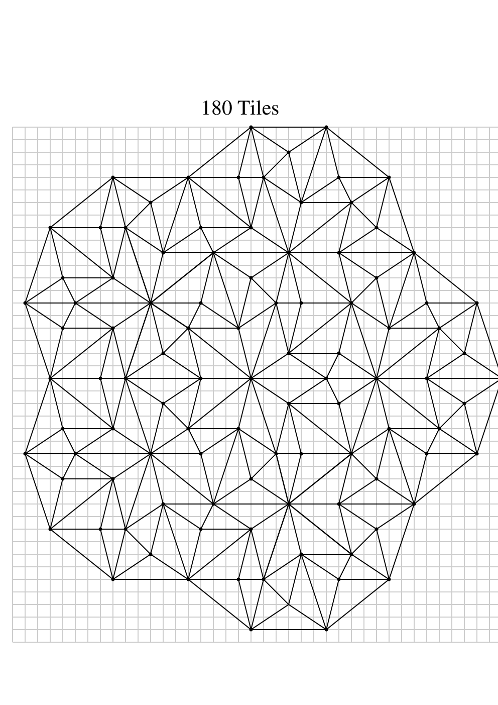
To avoid trivialities, we shall only consider nonperiodic tilings in this paper. Moreover, we shall assume that the tiles are polyhedra that meet full-face to full-face, and that there are only a finite set of tile types (a.k.a. prototiles) up to translation. Although these conditions may seem to be restrictive, any tiling that has finite local complexity with respect to translations is mutually locally derivable (MLD, see definition below) to a tiling meeting these conditions, via derived Voronoi tilings [Pr]. We also assume that our tiling spaces are minimal. This is equivalent to the condition that each patch of each tiling appear in all other tilings with bounded gaps.

Deformations of tiling spaces were considered in [SW]. As detailed there, to describe the shape and size of each tile, one must specify the displacement vector that corresponds to each edge of each prototile. If, somewhere in the tiling, translations of two prototiles meet along a common edge, then those two edges must have the same associated displacement vector. Moreover, the sum of the displacement vectors around each tile must be zero. Each deformation thus corresponds to a solution of a homogeneous linear system of equations subject to additional conditions which are open in the solution space: the sequence of edges around a tile does not cross itself and has winding number +1 and bounds a $2$-cell of a tile. If $d>2$ we also require the edges of a $2$-cell to be coplanar, and in general for all the edges of a $k$-cell of a tile to lie in a $k$-dimensional hyperplane of ${\mathbb{R}}^{d}$.

Put another way, the shapes of the prototiles are determined by a function $f$ from the set of prototile edges (modulo certain identifications) to ${\mathbb{R}}^{d}$. This function may be viewed as a 1-cochain on the CW-complex obtained by taking the disjoint union of all the prototiles, modulo the identification of edges (and other structures of dimension less than $d$) where tiles can meet. This is precisely the complex $\Gamma$ considered by Anderson and Putnam in their computation of topological invariants of substitution tiling spaces [AP]. (The Anderson-Putnam complex is defined for all translationally finite tilings, although it has been applied primarily to substitution tilings. See [G] for applications in a more general context.) That is, $f\in C^{1}(\Gamma,{\mathbb{R}}^{d})=Hom(C_{1}(\Gamma),{\mathbb{R}}^{d})$, and we may think of “shape space” as a subset of $C^{1}(\Gamma,{\mathbb{R}}^{d})$. (See, e.g., [M] for background on (co)homology.)

We denote vectors by bold-face roman letters, tiling spaces by ${\mathcal{T}}$ with appropriate subscripts, individual tilings by roman letters from the end of the alphabet (usually $x$ or $y$), and shape parameters by $f$ or $g$. The translate of the tiling $x$ by ${\bf z}\in{\mathbb{R}}^{d}$ is denoted $x-{\bf z}$.

Fix a tiling space ${\mathcal{T}}$, and consider deformations of this space. For any choice $f$ of edge vectors meeting the above requirements, we can consider tilings whose tiles are described by these edge vectors, but whose combinatorics (which tiles meet and how) are the same as the original tilings in ${\mathcal{T}}$. Let $\mathcal{T}_{f}$ denote the space of such deformed tilings, on which ${\mathbb{R}}^{d}$ acts naturally by translation. The primary focus of this paper is the extent to which the dynamical system $\mathcal{T}_{f}$ depends on the function $f$. If all we care about is the topological space, a theorem of [SW] shows that it doesn’t:

But what about dynamics? In a previous paper [CS] we showed how 1-dimensional substitution tiling space dynamics depend on the lengths of the tiles. Here we extend that analysis to higher dimensions, and also recast our 1-dimensional results in terms of topological invariants. One natural question is when two tiling spaces have topologically conjugate dynamics. Another is when they have dynamics that are intertwined by a local map. This involves the notion of mutual local derivability, first introduced in [BSJ].

Let $x$ and $y$ be two tilings, possibly with different sets of prototiles. The tiling $y$ is said to be locally derivable from $x$ if there exists a length $R$ such that, if ${\bf z}_{1},{\bf z}_{2}\in{\mathbb{R}}^{d}$ and $x-{\bf z}_{1}$ agrees with $x-{\bf z}_{2}$ on a ball of radius $R$ around the origin, then $y-{\bf z}_{1}$ agrees with $y-{\bf z}_{2}$ on a ball of radius 1 around the origin. In other words, the type and exact placement of the tile at a point ${\bf z}$ in $y$ depends only on the patch of radius $R$ around ${\bf z}$ in $x$. If $y$ is locally derivable from $x$ and $x$ is locally derivable from $y$, then $x$ and $y$ are said to be mutually locally derivable (MLD) tilings.

The MLD concept extends to tiling spaces. If $x$ and $y$ are MLD tilings, then the closure of the translational orbit of $x$ is topologically conjugate to the closure of the translation orbit of $y$, via a conjugacy that takes $x$ to $y$, and thus depends only on local data. More generally, we say that two tiling spaces ${\mathcal{T}}$ and ${\mathcal{T}}^{\prime}$ are MLD if there exists a topological conjugacy $\phi:{\mathcal{T}}\mapsto{\mathcal{T}}^{\prime}$ such that, for some $R$, the patch of size 1 around the origin in $\phi(x)$ can be determined exactly from the patch of size $R$ around the origin in $x$, and the patch of size 1 in $x$ can be determined exactly from the patch of size $R$ in $\phi(x)$. This is a natural generalization of the concept of “sliding block codes” for subshifts. However, while all continuous maps of subshifts are sliding block codes (see, e.g., [LM]), there exist topologically conjugate tiling spaces that are not MLD [RS, Pe, CS].

In Section 2, we construct a natural map ${\mathcal{I}}$ from the space of shape parameters to the Cech cohomology group $H^{1}({\mathcal{T}},{\mathbb{R}}^{d})$ ($=H^{1}({\mathcal{T}},{{\mathbb{Z}}})\otimes{\mathbb{R}}^{d}$) and show that the dynamical properties of ${\mathcal{T}}_{f}$ depend only on ${\mathcal{I}}(f)$:

Furthermore, we define a condition on $H^{1}({\mathcal{T}},{\mathbb{R}})$ (and by extension, $H^{1}({\mathcal{T}},{\mathbb{R}}^{d})$) called “asymptotic negligibility”. Roughly speaking, a deformation is asymptotically negligible if, up to an arbitrarily small error, it does not change the return vectors of large patches in a tiling. We then prove

Rescaling a tiling, or more generally applying a linear transformation, does not change the qualitative dynamical properties of the tiling space, such as mixing, minimality, or diffractivity. We therefore consider when a tiling space ${\mathcal{T}}_{f}$ is topologically conjugate to a linear transformation of a tiling space ${\mathcal{T}}_{g}$. Since linear transformations act naturally on the ${\mathbb{R}}^{d}$ factor of $H^{1}({\mathcal{T}},{\mathbb{R}}^{d})$ we have:

In Section 3 we specialize to nonperiodic tilings made from a primitive substitution, or a primitive substitution-with-amalgamation. The resulting spaces are orbit closures of self-similar or pseudo-self-similar tilings, respectively, in the terminology of [So1, So2, PS]. An essential object of study is the action of the substitution on the tiling space itself, and therefore on $H^{1}({\mathcal{T}},{\mathbb{R}}^{d})$. We decompose $H^{1}({\mathcal{T}},{\mathbb{R}}^{d})$ into (generalized) eigenspaces of the substitution operator. Let $S({\mathcal{T}})$ be the span of the (generalized) eigenvectors with eigenvalue strictly less than one in magnitude. We show that the set of asymptotically negligible classes is precisely $S({\mathcal{T}})$, and prove the following local converse to Theorem 1.3:

If there is a pseudo-self-similar tiling in ${\mathcal{T}}_{f}$, then ${\mathcal{I}}(f)$ is a Perron-Frobenius eigenvector of the substitution applied to $H^{1}({\mathcal{T}},{\mathbb{R}}^{d})$. The Perron-Frobenius eigenspace, denoted $PF({\mathcal{T}})$, is $d^{2}$ dimensional, and precisely equals $L{\mathcal{I}}(f)$, where $L$ ranges over all linear transformations of ${\mathbb{R}}^{d}$. Corollary 1.4 has the following simple restatement for substitution tilings:

In particular, if $H^{1}({\mathcal{T}},{\mathbb{R}}^{d})=PF({\mathcal{T}})\oplus S({\mathcal{T}})$, then all choices of shape give rise to conjugate dynamics, up to linear transformation. This case is the natural generalization, to higher dimensions, of Pisot substitutions.

For the space of Penrose tilings, $H^{1}({\mathcal{T}},{{\mathbb{Z}}})={{\mathbb{Z}}}^{5}$ [AP], so $H^{1}({\mathcal{T}},{\mathbb{R}}^{2})$ is 10-dimensional. The eigenvalues of the substitution are the golden mean $\tau$, with multiplicity 4, $1-\tau$ with multiplicity 4, and $-1$ with multiplicity 2. However, the $-1$ eigenspace is odd under rotation by 180 degrees, while the $\tau$ and $1-\tau$ eigenspaces are even [ORS]. Any choice of shapes that preserves the (statistical) 2-fold rotational symmetry of the Penrose tiling must not involve the $-1$ eigenspace. As a result, the tiling space constructed from the tiling of figure 2 is topologically conjugate to a linear transformation applied to the undistorted Penrose tiling space.

The techniques of Section 3 require recognizability, and hence draw heavily on Solomyak’s generalization [So2] of the work of Mossé on 1-dimensional subshifts [M1, M2].

In Section 4 we study the spectra of substitution tilings and their deformations. We provide general criteria for the existence of point spectrum of translations acting on ${\mathcal{T}}_{f}$, similar in spirit to criteria found in [So1] for self-similar tilings and to criteria in [CS] for 1-dimensional substitution tiling spaces and their deformations. We also provide constraints on the form of that spectrum, in terms of the aforementioned decomposition of ${\mathcal{I}}(f)$ into eigenspaces of the substitution operator. In particular, we show:

Finally, in Section 5 we revisit the problem in one dimension, and recast the results of [CS] in topological terms.

To define the map ${\mathcal{I}}$ we first recall the inverse limit structure of tiling spaces, developed by Anderson and Putnam [AP] for substitution tilings, and generalized by Gähler [G] to apply to all translationally finite tilings. (See [BBG] for an alternate approach, and [ORS, Sa, BG] for further generalizations).

We first construct a complex $\Gamma$ by taking the disjoint union of prototiles in the tiling, modulo identification of edges where tiles can meet. If somewhere in a tiling, edge $i$ of a tile of type $A$ is coincident with edge $j$ of a tile of type $B$, then we identify edge $i$ of $A$ with edge $j$ of $B$ in the complex. (If $d>2$ we also identify coincident faces and other structures of dimension up to $d-1$.)

We may also rewrite the tiling in terms of collared tiles, labeling each tile $t$ by the patch consisting of all tiles that touch $t$. Applying the construction of the previous paragraph to the collared tiles gives a complex $\Gamma^{(1)}$. Collaring the collared tiles and applying the construction gives a complex $\Gamma^{(2)}$, and more generally applying the construction to $k$-times collared tiles gives a complex $\Gamma^{(k)}$.

There is a natural “forgetful” map $\alpha_{0}$ from $\Gamma^{(1)}$ to $\Gamma$ that simply ignores the collaring, and likewise a forgetful map $\alpha_{k}:\Gamma^{(k+1)}\mapsto\Gamma^{(k)}$. The inverse limit of the sequence of maps and spaces

is isomorphic to the tiling space ${\mathcal{T}}$ [G]. A point in $\Gamma$ tells how to place a tile around the origin. A point in $\Gamma^{(1)}$ tells how to place a collared tile, i.e., a tile and its nearest neighbors. As $k$ increases, the points in $\Gamma^{(k)}$ tell how to place larger and larger patches around the origin, and the entire sequence $(x_{0},x_{1},\ldots)$ with $x_{i}\in\Gamma^{(i)}$ and $x_{i}=\alpha_{i}(x_{i+1})$ tells how to place a complete tiling.

We have already seen that the a shape parameter $f$ is a vector-valued 1-cochain in $\Gamma$. In fact, for any tile, $\delta f(t)=f(\partial t)=0$, since this is the sum of the edge vectors around the tile $t$. Thus $f$ is a cocycle, and defines a cohomology class $[f]\in H^{1}(\Gamma,{\mathbb{R}}^{d})$. Let $r_{k}:{\mathcal{T}}\mapsto\Gamma^{(k)}$ be the projection of the tiling space to the $k$th approximant. Define ${\mathcal{I}}(f)=r_{0}^{*}[f]\in H^{1}({\mathcal{T}},{\mathbb{R}}^{d})$.

Let $\pi_{k}=\alpha_{0}\circ\alpha_{1}\circ\cdots\circ\alpha_{k-1}:\Gamma^{(k)}\mapsto\Gamma$. If ${\mathcal{I}}(f)={\mathcal{I}}(g)$, then for some finite $k$, $\pi_{k}^{*}[f]-\pi_{k}^{*}[g]=0$, so $\pi_{k}^{*}f-\pi_{k}^{*}g=\delta\beta$ for some $\beta\in C^{0}(\Gamma^{(k)},{\mathbb{R}}^{d})$. Now each vertex ${\bf v}$ in a tiling in ${\mathcal{T}}_{f}$ maps to a unique vertex in $\Gamma^{(k)}$, the map being determined by a ball of size $(k+1)A$ around ${\bf v}$, where $A$ is the diameter of the largest prototile. Moving each vertex ${\bf v}$ by $-\beta({\bf v})$, and linearly interpolating the edges between vertices, converts a tiling in ${\mathcal{T}}_{f}$ to a tiling in ${\mathcal{T}}_{g}$. $\square$

For a tiling $x\in{\mathcal{T}}$, a recurrence is an ordered pair $({\bf z}_{1},{\bf z}_{2})$ of points in $x$ such that ${\bf z}_{1}$ is a point in a tile and ${\bf z}_{2}$ is the corresponding point of a translate of that tile and such that there exist balls around ${\bf z}_{1}$ and ${\bf z}_{2}$ that agree (up to translation by ${\bf z}_{2}-{\bf z}_{1}$, of course). If $r$ is the supremum of the radii of the balls around ${\bf z}_{1}$ and ${\bf z}_{2}$ that agree, then we say the recurrence has size $r$. Each path along edges from ${\bf z}_{1}$ to ${\bf z}_{2}$ projects to a closed loop in $\Gamma$, and hence to a closed chain in $C_{1}(\Gamma)$. Different paths from ${\bf z}_{1}$ to ${\bf z}_{2}$ correspond to homologous chains. The class in $H_{1}(\Gamma)$ of a recurrence is called a recurrence class. Note that recurrences of size greater than $(k+1)A$, where $A$ is the diamater of the largest prototile, also project to closed paths in $\Gamma^{(k)}$ and define classes in $H_{1}(\Gamma^{(k)})$. Since the tiling space ${\mathcal{T}}$ is assumed to be minimal, the set of recurrence classes is the same for every tiling in the space, and so we can speak of the recurrence classes of the tiling space.

An element $\eta$ of $H^{1}(\Gamma^{(k)},{\mathbb{R}})$, or of $H^{1}(\Gamma^{(k)},{\mathbb{R}}^{d})$, is said to be asymptotically negligible if, for each $\epsilon>0$ there exists a constant $R_{\epsilon}$ such that $\eta$, applied to any homology class that can be represented by a recurrence of size greater than $R_{\epsilon}$, is less than $\epsilon$ in magnitude. A class in $H^{1}({\mathcal{T}},{\mathbb{R}}^{d})$ is asymptotically negligible if it is the pullback of an asymptotically negligible class in $H^{1}(\Gamma^{(k)},{\mathbb{R}}^{d})$ for some finite $k$. It is clear that any linear combination of asymptotically negligible classes is asymptotically negligible, so these classes form a subspace of $H^{1}({\mathcal{T}},{\mathbb{R}}^{d})$, denoted $N({\mathcal{T}})$.

For every vertex ${\bf v}$ in $x$ there is a path $p_{\bf v}$ from the origin to ${\bf v}$ along edges, and the location of ${\bf v}$ is precisely $f(p_{\bf v})$. In $\phi(x)$ we place the corresponding vertex at $g(p_{\bf v})$. The path $p_{\bf v}$ is not uniquely defined, but different choices differ by boundaries, so the values of $f(p_{\bf v})$ and $g(p_{\bf v})$ are uniquely determined. Once the location of the vertices of $\phi(x)$ are specified, constructing the edges and tiles is straightforward.

This defines $\phi(x)$. For ${\bf z}\in{\mathbb{R}}^{d}$, let $\phi(x-{\bf z})=\phi(x)-{\bf z}$. It remains to show that $\phi$ is uniformly continuous on the orbit of $x$, and hence can be extended to all of ${\mathcal{T}}$.

Suppose that ${\bf z}_{1}$ and ${\bf z}_{2}$ are vertices in $x$ such that $x-{\bf z}_{1}$ and $x-{\bf z}_{2}$ agree on a large ball around the origin. Note that $\phi(x)-g(p_{{\bf z}_{1}})$ agrees exactly with $\phi(x)-g(p_{{\bf z}_{2}})$ on a large ball around the origin. Since $f-g$ is asymptotically negligible, $f(p_{{\bf z}_{2}})-f(p_{{\bf z}_{1}})$ is very close to $g(p_{{\bf z}_{2}})-g(p_{{\bf z}_{1}})$, so $\phi(x-{\bf z}_{1})=\phi(x)-f(p_{{\bf z}_{1}})$ agrees with $\phi(x-{\bf z}_{2})=\phi(x)-f(p_{{\bf z}_{2}})$ on a large ball around the origin, up to a small translation, of size $f(p_{{\bf z}_{2}})-f(p_{{\bf z}_{1}})-\left(g(p_{{\bf z}_{2}})-g(p_{{\bf z}_{1}})\right)$. Since this translation can be made arbitrarily small by making the recurrence of sufficiently large size (independent of the choice of ${\bf z}_{1}$ and ${\bf z}_{2}$), $\phi$ is uniformly continuous on the orbit of $x$.

To see that $\phi$ is invertible, construct a semi-conjugacy $\phi^{\prime}:{\mathcal{T}}_{g}\mapsto{\mathcal{T}}_{f}$ by the same procedure, with the roles of $f$ and $g$ reversed, and with $\phi(x)$ as the reference tiling. Since $\phi^{\prime}(\phi(x))=x$, it is clear that $\phi$ and $\phi^{\prime}$ are inverses. $\square$

Note that ${\mathcal{T}}_{f}$ and ${\mathcal{T}}_{g}$ are typically not MLD. If two tilings in ${\mathcal{T}}_{f}$ agree on a large ball around the origin, the corresponding tilings in ${\mathcal{T}}_{g}$ agree on a large ball up to a small translation. Only if $f-g$ vanishes on large recurrence classes do they agree without translation. In that case, however, the following theorem shows that ${\mathcal{I}}(f)={\mathcal{I}}(g)$, and we are back in the situation of Theorem 1.2.

Now consider our class $\beta$, and represent it as a closed P-equivariant 1-form $\rho$. Let $\gamma({\bf z})=\int_{0}^{\bf z}\rho$. It is clear that $\rho=d\gamma$, and the condition that $\beta$ vanishes on large recurrence classes implies that $\gamma$ is P-equivariant with radius $R$. Thus $\rho$ represents the zero class in $H^{1}({\mathcal{T}},{\mathbb{R}})$. $\square$

We now specialize to substitution tiling spaces, where we can obtain sharper results. In this section we identify the asymptotically negligible cohomology classes and prove Theorem 1.5.

A substitution tiling system is determined by a substitution $\sigma$ from the set of prototiles to the set of finite patches, such that for each prototile $t$, the tiles of $\sigma(t)$ do not overlap, and such that their union is the rescaled prototile $\lambda t$, where $\lambda$ is a fixed “stretching factor”. For example, in the “chair” tiling, there are four prototiles: One is the L-shaped tile of figure 3 and the others are this tile rotated by $\pi/2$, $\pi$ and $3\pi/2$. The substitution map is shown in figure 3. We extend the map $\sigma$ to patches, dilating the entire patch by a factor of $\lambda$ and replacing each dilated tile $\lambda t_{i}$ with $\sigma(t_{i})$. For each prototile $t$ we have a sequence of patches $t,\sigma(t),\sigma^{2}(t),\cdots$. A tiling $x$ of ${\mathbb{R}}^{d}$ by prototiles is called admissible if for every finite patch $P$ of $x$, there exists a prototile $t$ and an integer $n$ such that $P$ is a translate of a subpatch of $\sigma^{n}(t)$. The substitution tiling space ${\mathcal{T}}$ is then the set of all admissible tilings, and $\sigma$ extends to a continuous map ${\mathcal{T}}\mapsto{\mathcal{T}}$.

We assume that the substitution is primitive. That is, there exists an integer $n$ such that, for any two (possibly identical) prototiles $t_{1}$ and $t_{2}$, $\sigma^{n}(t_{1})$ contains a copy of $t_{2}$. This ensures that ${\mathcal{T}}$ is minimal. Furthermore, we assume that ${\mathcal{T}}$ is non-periodic. There does not exist a tiling $x\in{\mathcal{T}}$ and a nonzero ${\bf z}\in{\mathbb{R}}^{d}$ with $x-{\bf z}=x$. By a theorem of Solomyak [So2], extending previous work by Mossé [M1, M2], this implies that $\sigma:{\mathcal{T}}\mapsto{\mathcal{T}}$ is a homeomorphism. There then exists a “recognition length” $D$ such that, if $x$ and $y$ are tilings that agree on a ball of radius $r>D$ about a point ${\bf z}\in{\mathbb{R}}^{d}$, then $\sigma^{-1}(x)$ and $\sigma^{-1}(y)$ agree on the tile(s) containing the point ${\bf z}/\lambda$.

In every substitution tiling space there exists a fixed point of some power of the substitution. Replacing $\sigma$ with a power of $\sigma$ does not change the tiling space, so we can assume, without loss of generality, that there is a tiling $x$ with $\sigma(x)=x$. Such a tiling is called “self-similar”, and has the property that $\lambda x$ is a tiling by large tiles, each of which is a union of tiles of $x$. Some authors begin by defining self-similar tilings by this property, and then take ${\mathcal{T}}$ to be the closure of the translational orbit of $x$.

Closely related to self-similar tilings are pseudo-self-similar tilings. A tiling $x$ is pseudo-self-similar if, for some scaling factor $\lambda$, $\lambda x$ and $x$ are MLD. Natalie Priebe Frank and Boris Solomyak [PS] have shown that every pseudo-self-similar planar tiling with polygonal tiles is MLD to a self-similar tiling. However, the tiles of the self-similar tiling may not be polygonal; rather, they may have fractile boundaries. Conversely, Natalie Priebe Frank [Pr] showed (in arbitrary dimension) that each self-similar tiling (with tiles of arbitrary shape) is MLD to a pseudo-self-similar tiling with polyhedral tiles meeting full-face to full-face.

Orbit closures of pseudo-self-similar tilings may also be viewed as coming from a substitution-with-amalgamation. A substitution-with-amalgamation is the composition of a linear rescaling and a local map. The local map is a prescription for replacing each rescaled prototile $\lambda t$ by a collection of tiles, such that the resulting tiles do not overlap and do not leave any gaps. As with an ordinary substitution, $\sigma$ extends to a homeomorphism ${\mathcal{T}}\mapsto{\mathcal{T}}$. In a (strict) substitution tiling, each rescaled prototile $\lambda t$ in $\lambda x$ is a union of tiles of $\sigma(x)$, but in a substitution-with-amalgamation, the tiles of $\sigma(x)$ may stick in and out of the tiles of $\lambda x$.

An example of a substitution-with-amalgamation, for a tiling by marked hexagonal tiles, is shown in figure 4. Each small hexagon is rescaled by a linear factor of two, and the resulting large hexagon is replaced by four small hexagons. The union of the four small hexagons is not the corresponding large hexagon, yet the small hexagons associated to all the large hexagons yield a tiling of the plane, without gaps or overlaps.

In this section we assume that ${\mathcal{T}}$ is a nonperiodic substitution tiling space derived from a substitution-with-amalgamation $\sigma$. Since $\sigma$ maps ${\mathcal{T}}$ to ${\mathcal{T}}$, it induces a pullback map: $\sigma^{*}:H^{1}({\mathcal{T}},{\mathbb{R}}^{d})\mapsto H^{1}({\mathcal{T}},{\mathbb{R}}^{d})$. We decompose $H^{1}({\mathcal{T}},{\mathbb{R}}^{d})$ into (generalized) eigenspaces of $\sigma^{*}$. The largest eigenvalue, denoted $\lambda_{PF},$ equals the stretching factor and has multiplicity $d^{2}$. (In terms of P-equivariant cohomology, a basis for this space is $dz^{i}\otimes e_{j}$, where $e_{1},\ldots,e_{d}$ is the standard basis for ${\mathbb{R}}^{d}$ and $z^{1},\ldots z^{d}$ are Cartesian coordinates.) The corresponding eigenspace is denoted $PF({\mathcal{T}})$. The span of the (generalized) eigenvectors with eigenvalues of magnitude strictly less than 1 is denoted $S({\mathcal{T}})$.

Anderson and Putnam’s results [AP] were originally stated for substitutions without amalgamation, but apply also to substitutions with amalgamation. The substitution $\sigma$ induces a map from $\Gamma^{(1)}$ to itself, and ${\mathcal{T}}$ is the inverse limit of the sequence of maps:

The cohomology $H^{1}({\mathcal{T}},{\mathbb{R}}^{d})$ is then the direct limit of $H^{1}(\Gamma^{(1)},{\mathbb{R}}^{d})$ under $\sigma^{*}:H^{1}(\Gamma^{(1)},{\mathbb{R}}^{d})\mapsto H^{1}(\Gamma^{(1)},{\mathbb{R}}^{d})$. Nonzero eigenspaces of $\sigma^{*}$ applied to $H^{1}({\mathcal{T}},{\mathbb{R}}^{d})$ correspond to nonzero eigenspaces of $\sigma^{*}$ applied to $H^{1}(\Gamma^{(1)},{\mathbb{R}}^{d})$. The only difference between $H^{1}({\mathcal{T}},{\mathbb{R}}^{d})$ and $H^{1}(\Gamma^{(1)},{\mathbb{R}}^{d})$ is that $H^{1}(\Gamma^{(1)},{\mathbb{R}}^{d})$ may contain a (generalized) zero-eigenspace of $\sigma^{*}$, while $H^{1}({\mathcal{T}},{\mathbb{R}}^{d})$ does not.

This decomposition into eigenspaces of $\sigma^{*}$ makes it easy to identify the asymptotically negligible classes.

To show that $S({\mathcal{T}})\subset N({\mathcal{T}})$, note that every recurrence class $[p_{z}]$ can be written as a sum

with only a finite number of nonzero terms, and with all the $[p_{j}]$’s belonging to a fixed bounded subset $U$ of $H_{1}(\Gamma^{(1)})$. (The argument is essentially that found in [So2, Proof of Lemma 3.2] and is not repeated here.) If the recurrence has size greater than $D(1+\lambda_{PF}+\cdots+\lambda_{PF}^{n-1})$ where $D$ is the recognition length, then the first $n$ terms are zero.

Suppose that $\beta$ is an eigenvector of $\sigma^{*}$ with eigenvalue $\lambda$ of magnitude strictly less than 1. Let $K$ be larger than the greatest value that $\beta$ takes on $U$. Then for any recurrence class $[p_{z}]$, $|\beta(p_{z})|<K/(1-|\lambda|)$. If $p_{z}$ has size greater than $D(1+\lambda_{PF}+\cdots+\lambda_{PF}^{n-1})$, then $|\beta(p_{z})|<K|\lambda|^{n}/(1-|\lambda|)$. Thus $\beta$ is asymptotically negligible. Since linear combinations of asymptotically negligible classes are asymptotically negligible, $S({\mathcal{T}})\subset N({\mathcal{T}})$.

When $\sigma^{*}$ is not diagonalizable, the analysis is only slightly more complicated. The expansion of $\beta(\sigma^{n}(p_{j}))$ may involve $n$-th powers of eigenvalues times polynomials in $n$, rather than just $n$-th powers of eigenvalues. However, the conclusions are unchanged. $\square$

Theorem 3.2 gives sufficient conditions for two tiling spaces to be conjugate. For infinitesimal deformations, these conditions are also necessary:

The remainder of this section is devoted to proving Theorem 3.3. To prove the theorem we must understand the extent to which patterns in ${\mathcal{T}}$ can repeat themselves. For each recurrence $({\bf z}_{1},{\bf z}_{2})$, let the degree of the recurrence be its size divided by $|{\bf z}_{2}-{\bf z}_{1}|$. For fixed $p>0$, we show that the recurrence classes corresponding to recurrences with degree $p$ or greater can be grouped into a finite number of families, and we construct a conjugacy invariant from the asymptotic displacements of these recurrences. Comparing these invariants for different shape parameters then gives necessary conditions for conjugacy.

It is convenient to work with explicit matrices. The set of integer linear combinations of recurrence classes of size at least $2A$ (where $A$ is the diameter of the largest tile) is a sub-lattice of $H_{1}(\Gamma^{(1)})$. Let $\{a_{1},\ldots,a_{s}\}$ be a basis for this sub-lattice. Since $\sigma$ maps recurrences to recurrences, it maps the lattice to itself. Let $M$ be the matrix of this map relative to the basis $\{a_{1},\ldots,a_{s}\}$. Note that the entries of $M$ are integers. The matrix $M$ will play a role similar to that of the substitution matrix in one-dimensional substitutions. For each recurrence class in $H_{1}(\Gamma^{(1)})$, the corresponding recurrence vector in ${{\mathbb{Z}}}^{s}$ is the decomposition of the class in the $\{a_{1},\ldots,a_{s}\}$ basis. For any shape parameter $f$, let ${\bf L}_{f}=(f(a_{1}),\ldots,f(a_{s}))$ be the (${\mathbb{R}}^{d}$-valued row) vector that gives the displacements, in ${\mathbb{R}}^{d}$, corresponding to lifts of the various loops. For a recurrence with vector ${\bf v}$, the corresponding displacement is ${\bf L}_{f}{\bf v}$. The Euclidean length of ${\bf L}_{f}{\bf v}$ is called the length of ${\bf v}$, and denoted $|{\bf v}|_{f}$. We call ${\bf L}_{f}$ the shape vector of ${\mathcal{T}}_{f}$.

Let ${\mathcal{T}}_{0}$ be a tiling space whose shape vector ${\bf L}_{0}$ is a left Perron-Frobenius eigenvector of $M$. This can be the original substitution tiling space, a linear transformation applied to the original space, or a space that is MLD to such a linear transformation. In all such cases, there exists a pseudo-self-similar tiling in the space, and we call the space itself pseudo-self-similar.

If ${\bf v}$ is a recurrence vector of degree $p$ in ${\mathcal{T}}_{0}$, corresponding to a recurrence $({\bf z}_{1},{\bf z}_{2})$ in a tiling $x$, then $M{\bf v}$ is also a recurrence vector of degree at least $p$, corresponding to the recurrence $(\lambda_{PF}{\bf z}_{1},\lambda_{PF}{\bf z}_{2})$ in the tiling $\sigma(x)$. Both the size of the matching balls around ${\bf z}_{1}$ and ${\bf z}_{2}$ and the distance from ${\bf z}_{1}$ to ${\bf z}_{2}$ get stretched by the same factor $\lambda_{PF}$ in the substitution. Thus each recurrence vector of degree $p$ gives rise to a family of recurrence vectors $M^{k}{\bf v}$. The following theorem limits the number of such families.

Repeating the process, we find recurrence vectors ${\bf v}_{i}$ such that $M{\bf v}_{i}={\bf v}_{i-1}$ and ${\bf v}_{i}$ is a recurrence vector of degree at least

Now pick $\epsilon<p$. We have shown that every recurrence vector of degree at least $p$ is of the form $M^{k}{\bf v}_{i}$, where ${\bf v}_{i}$ is a recurrence vector of degree at least $p-\epsilon$, and where $|{\bf v}_{i}|_{0}$ is bounded by $\frac{D\lambda_{PF}}{\epsilon(\lambda_{PF}-1)}$. However, by finite local complexity, there are only a finite number of recurrence vectors of this length. $\square$

As defined, the degree of a recurrence vector depends on the shape vector of the tiling space. Indeed, since linear transformations do not preserve lengths or ratios of lengths, the degree of a recurrence vector in two pseudo-self-similar tiling spaces may not be the same. However, for any tiling space ${\mathcal{T}}_{f}$, the degrees of large recurrence vectors are approximately the same as that of some pseudo-self-similar tiling space:

If $\lambda_{2}$ is the second largest eigenvalue in magnitude, then in recurrences of the form $M^{n}{\bf v}$, $|r_{\bf v}-1|$ goes to 0 as $\left(\lambda_{2}/\lambda_{PF}\right)^{n}$. Moreover, this convergence is uniform in $n$ for all recurrences, because all non-zero recurrences are longer than the diameter of a ball that can fit in each prototile. As indicated in the proof of theorem 3.1, given any $N$, all recurrences of sufficient length are sums of recurrences of the form $M^{n}{\bf v}$ with $n>N$, and so the result follows. $\square$

Theorem 3.4 showed there there are only a finite number of families of recurrence vectors of a given degree for a self-similar tiling. Lemma 3.6 extends that result to all tiling spaces.

We now construct a topological invariant from the asymptotic displacements ${\bf L}_{f}{\bf v}$ of large recurrence vectors ${\bf v}$.

In other words, up to small errors in the degree and the displacement that vanish in the limit of large recurrence classes, the degrees and displacements of the recurrence classes are conjugacy invariants.

Now let ${\bf v}$ be a recurrence vector of degree $p$ for ${\mathcal{T}}_{f}$, representing a recurrence $({\bf z}_{1},{\bf z}_{2})$ in a tiling $x\in{\mathcal{T}}_{f}$. Then $x-{\bf z}_{1}$ and $x-{\bf z}_{2}$ agree on a ball of radius $p|{\bf v}|_{f}$ about the origin, so $\phi(x)-{\bf z}_{1}$ and $\phi(x)-{\bf z}_{2}$ agree on a ball of radius $p|{\bf v}|_{f}-D_{0}$, up to translation of size at most $h(R)$. Thus there exists a point ${\bf z}_{3}$, within $h(D)$ of ${\bf z}_{2}$, such that ${\bf v}^{\prime}=[({\bf z}_{1},{\bf z}_{3})]$ is a recurrence class of degree at least $\frac{p|{\bf v}|_{f}-D_{0}}{|{\bf v}|_{f}+h(D)}$ in ${\mathcal{T}}_{g}$. For $D$ large enough, this is greater than $p-\epsilon_{1}$ and $|{\bf L}_{f}{\bf v}-{\bf L}_{g}{\bf v}^{\prime}|<h(R)$ is less than $\epsilon_{2}$. $\square$

Note that all recurrence vectors are recurrence vectors of some positive degree. We can therefore pick $p_{0}$ such that the integer span of the recurrence vectors of degree at least $p_{0}$ is an $s$-dimensional sublattice of ${{\mathbb{Z}}}^{s}$. Pick $\epsilon$ small enough (and adjust $p_{0}$ by up to $\epsilon$, if necessary) so that all the families of recurrence vectors of degree at least $p_{0}-\epsilon$ are also families of recurrence vectors of degree at least $p_{0}+\epsilon$. Let ${\bf v}_{1},\ldots,{\bf v}_{k}$ be generating vectors of those families. By multiplying by appropriate powers of $M$, these can be chosen so that all of the magnitudes of the displacements $|M^{k}{\bf v}_{i}|_{f}$ are within a factor of $\lambda_{PF}$ of one another for large $k$.

Now pick a neighborhood $U_{\epsilon}$ of $f$ in $C^{1}(\Gamma,{\mathbb{R}}^{d})$ small enough that, if $g^{\prime}\in U_{\epsilon}$, then every recurrence class in ${\mathcal{T}}_{f}$ of degree at least $p_{0}+\epsilon$ is also a recurrence class in ${\mathcal{T}}_{g^{\prime}}$ of degree at least $p_{0}$, and such that every recurrence class in ${\mathcal{T}}_{g^{\prime}}$ of degree at least $p_{0}$ is a recurrence class in ${\mathcal{T}}_{f}$ of degree at least $p_{0}-\epsilon$. This insures that the families of recurrence classes of degree at least $p_{0}$ in the two tiling spaces are exactly the same.

If ${\mathcal{T}}_{f}$ and ${\mathcal{T}}_{g^{\prime}}$ are conjugate then, by Theorem 3.7, the displacements ${\bf L}_{f}M^{k}{\bf v}_{j}$ can be approximated by ${\bf L}_{g^{\prime}}M^{k^{\prime}}{\bf v}_{j^{\prime}}$ for some $k^{\prime},j^{\prime}$, and the approximation get successively better as $k\to\infty$. However, if $U_{\epsilon}$ is chosen small enough, the only values of $k^{\prime},j^{\prime}$ that come close to approximating are $k^{\prime}=k$ and $j^{\prime}=j$. Thus the limit of $({\bf L}_{f}-{\bf L}_{g^{\prime}})M^{k}{\bf v}_{j}$ must be zero. By Theorem 2.3, this implies that $(\sigma^{*})^{k}({\mathcal{I}}(f)-{\mathcal{I}}(g^{\prime}))$ approaches zero as $k\to\infty$, and hence that ${\mathcal{I}}(f)-{\mathcal{I}}(g^{\prime})\in S({\mathcal{T}})$.

Finally, let $U_{f}={\mathcal{I}}(U_{\epsilon})$. If ${\mathcal{I}}(g)\in U_{f}$, then ${\mathcal{T}}_{g}$ is MLD to a tiling space ${\mathcal{T}}_{g^{\prime}}$ with $g^{\prime}\in U_{\epsilon}$ and ${\mathcal{I}}(g^{\prime})={\mathcal{I}}(g)$. Since ${\mathcal{T}}_{g^{\prime}}$ is conjugate to ${\mathcal{T}}_{f}$, ${\mathcal{I}}(f)-{\mathcal{I}}(g)={\mathcal{I}}(f)-{\mathcal{I}}(g^{\prime})\in S({\mathcal{T}})$. $\square$

Now we turn to the topological point spectrum of substitution tiling spaces, by which we mean the eigenvalues of continuous eigenfuctions of the translation action. First we determine general criteria for a vector to be an eigenvalue for a continuous eigenfunction, and then we apply this criteria to some special cases, depending on the form of the matrix $M$ defined in Section 3. This eventually leads to criteria for topological weak mixing.

References

- [AP] J. E. Anderson and I. F. Putnam, Topological invariants for substitution tilings and their associated algebras. Ergodic Theory & Dynamical Systems 18 (1998), 509-537.
- [BBG] J. Bellissard, R. Benedetti, and J.-M. Gambaudo, Spaces of tilings, finite telescopic approximations and gap-labelling, to appear in Commun. Math. Phys.
- [BG] R. Benedetti and G.-M. Gambaudo, On the dynamics of -solenoids: applications to Delone sets, to appear in Ergodic Theory & Dynamical Systems 23 (2003) 673–691.
- [BSJ] M. Baake, M. Schlottmann and P. D. Jarvis, Quasiperiodic tilings with tenfold symmetry and equivalence with respect to local derivability. J. Physics A 24 (1991), 4637-4654.
- [CS] A. Clark and L. Sadun, When size matters: subshifts and their related tiling spaces. Ergodic Theory Dynamical Systems 23 (2003) 1043–1057.
- [G] F. Gähler, in preparation.
- [K] J. Kellendonk, Pattern-equivariant functions and cohomology, J. Phys. A 36 (2003) 5765–5772.
- [KP] J. Kellendonk and I. Putnam, in preparation.
- [LM] D. Lind and B. Marcus, An Introduction to Symbolic Dynamics and Coding, Cambridge University Press, NY (1995).
- [M1] B. Mossé, Puissances de mots et reconnaissabilité des points fixes d’une substitution. Theoret. Comput. Sci. 99 (1992), 327–334.
- [M2] B. Mossé, Reconnaissabilité des substitutions et complexité des suites automatiques. Bull. Soc. Math. France 124 (1996), 329–346.
- [M] J. R. Munkres, Elements of algebraic topology. Addison-Wesley Publishing Company, Menlo Park, CA, (1984).
- [ORS] N. Ormes, C. Radin, and L. Sadun, A homeomorphism invariant for substitution tiling spaces, Geom. Dedicata 90 (2002) 153–182.
- [Pe] K. Petersen, Factor maps between tiling dynamical systems, Forum Math. 11 (1999) 503–512.
- [Pr] N. M. Priebe, Towards a characterization of self-similar tilings in terms of derived Voronoi tesselations. Geom. Dedicata 79 (2000), 239–265.
- [PS] N. Priebe and B. Solomyak, Characterization of planar pseudo-self-similar tilings. Discrete Comput. Geom. 26 (2001), 289–306.
- [RS] C. Radin and L. Sadun, Isomorphism of hierarchical structures, Ergodic Theory & Dynamical Systems 21 (2001), 1239-1248.
- [Sa] L. Sadun, Tiling spaces are inverse limits, preprint 2002, math.DS/0210179 to appear in J. Math. Phys.
- [So1] B. Solomyak, Dynamics of self-similar tilings. Ergodic Theory & Dynamical Systems 17 (1997), 695–738; Corrections in 19 (1999), 1685.
- [So2] B. Solomyak, Non-periodicity implies unique composition for self-similar translationally-finite tilings. Discrete Comput. Geom. 20 (1998), 265–279.
- [SW] L. Sadun and R. F. Williams, Tiling spaces are Cantor set fiber bundles. Ergodic Theory Dynamical Systems 23 (2003), 307–316.