跳到论文正文
W Papers独立论文阅读器 arXiv:math/0305421 论文正文 计算阅读时间 · 0%
引用这篇论文根据当前论文元数据生成,正式投稿前建议核对。


License: Assumed arXiv.org perpetual non-exclusive license
arXiv:math/0305421v1 [math.NT] 29 May 2003

Higher-dimensional Dedekind sums and their bounds arising from the discrete diagonal of the nn-cubeThanks: The second author would like to thank the generous support of NSA Young Investigator grant MSPR-OOY-196

Matthias Beck Address: Department of Mathematical Sciences
Binghamton University (SUNY)
Binghamton, NY 13902-6000
USA
Email address: matthias@math.binghamton.edu
, Sinai Robins Address: Department of Mathematics
Temple University
Philadelphia, PA 19122
USA
Email address: srobins@math.temple.edu
and Shelemyahu Zacks Address: Department of Mathematical Sciences
Binghamton University (SUNY)
Binghamton, NY 13902-6000
USA
Email address: shelly@math.binghamton.edu
Abstract.

Higher-dimensional Dedekind sums are defined as a generalization of a recent 1-dimensional probability model of Dilcher and Girstmair to a dd-dimensional cube. The analysis of the frequency distribution of marked lattice points leads to new formulae in certain special cases, and to new bounds for the classical Dedekind sums. Upper bounds for the generalized Dedekind sums are defined in terms of 1-dimensional moments. In the classical two-dimensional case, the ratio of these sums to their upper bounds are cosines of angles between certain vectors of n-dimensional cones, conjectured to have a largest spacial angle of π/6\pi/6.

Key words and phrases: 
Dedekind sums, Cauchy-Schwartz inequality, frequency distributions, moments.

Counting pairs is the oldest trick in combinatorics… Every time we count pairs, we learn something from it.
Gil Kalai

1. Introduction

Historically, Dedekind sums first appeared in Dedekind’s transformation law of his η\eta-function [2]. Dedekind sums have since become an integral part of combinatorial geometry (lattice point enumeration [8]), algebraic number theory (class number formulae [7]), topology (signature defects of manifolds [4]), and algorithmic complexity (pseudo random number generators [5]). We begin by defining the classical Dedekind sum, whose basic ingredient is the sawtooth function

((x))={{x}−12 if ​x∉ℤ0 if ​x∈ℤ.((x))=\left\{\begin{array}[]{cl}\{x\}-\frac{1}{2}&\mbox{ if }x\not\in\mathbb{Z}\\ 0&\mbox{ if }x\in\mathbb{Z}\ .\end{array}\right.

Here {x}=x−⌊x⌋\{x\}=x-\left\lfloor{x}\right\rfloor denotes the fractional part of a real number xx.

For any two positive integers aa and bb, we define the classical Dedekind sum as

(1.1) s⁡(a,b)=∑k​ mod ​b((k​ab))​((kb)).s(a,b)=\sum_{k\text{ {\rm mod} }b}\left(\left(\frac{ka}{b}\right)\right)\left(\left(\frac{k}{b}\right)\right)\ .

Here the sum is over a complete residue system modulo bb.

The classic introduction to the arithmetic properties of the Dedekind sum is [9]. The Dedekind sums have recently been cast in a new light as essentially the second moments of an appealing probability model introduced by Dilcher and Girstmair [3]. They divide an interval of length aa into bb equal subintervals (“boxes”) and count the number of integers in each subinterval.

We generalize their approach by considering a dd-dimensional cube (d≥2d\geq 2) of side length a∈ℕa\in\mathbb{N}. Along the dd-dimensional main diagonal we mark the points with integer coordinates. The cube is now partitioned to b1b2⋯bdb_{1}b_{2}\cdots b_{d} rectangular parallelopipeds by dividing the jthj^{\text{th}} side of the cube to bjb_{j} equal length intervals. Each parallelopiped is given the coordinates (j1,j2,…,jd)(j_{1},j_{2},\dots,j_{d}) where jk=1,…,bk​(k=1,…,d)j_{k}=1,\dots,b_{k}\ (k=1,\dots,d). Let fa;b1,…,bd​(j1,…,jd)f_{a;b_{1},\dots,b_{d}}(j_{1},\dots,j_{d}) denote the number (frequency) of marked points along the main diagonal which belong to the (j1,j2,…,jd)(j_{1},j_{2},\dots,j_{d})-parallelopiped. The generalized Dedekind sums under consideration are

(1.2) Sd(a;𝐛)=Sd(a;b1,b2,…,bd)=1a∑k1=0b1−1⋯∑kd=0bd−1k1⋯kdfa;b1,…,bd(k1,…,kd),S_{d}(a;{\bf b})=S_{d}(a;b_{1},b_{2},\dots,b_{d})=\frac{1}{a}\sum_{k_{1}=0}^{b_{1}-1}\cdots\sum_{k_{d}=0}^{b_{d}-1}k_{1}\cdots k_{d}\,f_{a;b_{1},\dots,b_{d}}\left(k_{1},\dots,k_{d}\right),

a mixed moment for the fa;b1,…,bdf_{a;b_{1},\dots,b_{d}} distribution. In Section 2 we present basic definition and facts. We show that

(1.3) Sd(a;𝐛)=1a∑m=0a−1⌊m​b1a⌋⋯⌊m​bda⌋,S_{d}(a;{\bf b})=\frac{1}{a}\sum_{m=0}^{a-1}\left\lfloor{\frac{mb_{1}}{a}}\right\rfloor\cdots\left\lfloor{\frac{mb_{d}}{a}}\right\rfloor\ ,

For the case d=1d=1 we define the kthk^{\text{th}} moment as

(1.4) Mk​(a,b)=1a​∑m=0a−1⌊m​ba⌋k.M_{k}(a;b)=\frac{1}{a}\sum_{m=0}^{a-1}\left\lfloor\frac{mb}{a}\right\rfloor^{k}\ .

These moments are used in Sections 5 and 6 to provide, via the Cauchy-Schwartz inequality, upper bounds for Sd​(a,𝐛)S_{d}(a;{\bf b}).

The second moment M2​(a,b)M_{2}(a;b) is of special importance since it is connected with the classical Dedekind sum s⁡(a,b)s(a,b) according to the formula (see Section 2)

(1.5) M2​(a,b)=(b2+1)​(a−1)​(2​a−1)6​a2−(a−1)​b2​a−2​ba​s​(b,a).M_{2}(a;b)=\frac{(b^{2}+1)(a-1)(2a-1)}{6a^{2}}-\frac{(a-1)b}{2a}-\frac{2b}{a}\,s(b,a)\ .

By analyzing the structure of the univariate and bivariate frequency distributions (Section 3), we derive in Section 4 new formulae for M2​(a,b)M_{2}(a;b), in some special cases, and provide several types of lower and upper bounds. In Section 5 we analyze the ratio of S2​(a,b1,b2)S_{2}(a;b_{1},b_{2}) to its upper bound (M2​(a,b1)​M2​(a,b2))1/2\left(M_{2}(a;b_{1})M_{2}(a;b_{2})\right)^{1/2}. All these ratios R2​(a,b1,b2)R_{2}(a;b_{1},b_{2}) are empirically found to be greater or equal to R2​(5,2,3)=3/2R_{2}(5;2,3)=\sqrt{3}/2, leading to the following conjecture (see section 5.15.1 below):

Conjecture 1. For all a,b,c≥3a,b,c\geq 3,

(1.6) R2​(a,b,c)≥R2​(5,2,3)=32.R_{2}(a;b,c)\geq R_{2}(5;2,3)=\frac{\sqrt{3}}{2}\ .

Geometrically, S2​(a,b1,b2)S_{2}(a;b_{1},b_{2}) is an inner product of the vectors 𝐯b1=(⌊b1a⌋,⌊2​b1a⌋,…,⌊(a−1)​b1a⌋){\bf v}_{b_{1}}=\left(\left\lfloor{\frac{b_{1}}{a}}\right\rfloor,\left\lfloor{\frac{2b_{1}}{a}}\right\rfloor,\dots,\left\lfloor{\frac{(a-1)b_{1}}{a}}\right\rfloor\right) and 𝐯b2=(⌊b2a⌋,⌊2​b2a⌋,…,⌊(a−1)​b2a⌋){\bf v}_{b_{2}}=\left(\left\lfloor{\frac{b_{2}}{a}}\right\rfloor,\left\lfloor{\frac{2b_{2}}{a}}\right\rfloor,\dots,\left\lfloor{\frac{(a-1)b_{2}}{a}}\right\rfloor\right) in ℝa−1\mathbb{R}^{a-1}, and R2​(a,b1,b2)R_{2}(a;b_{1},b_{2}) is the cosine of the angle between these two vectors. It appears from both empirical and theoretical evidence that all these vectors, for a≥3,b1,b2≥2a\geq 3,\,b_{1},b_{2}\geq 2, are within a cone with largest possible angle of cos−1⁡(3/2)=π/6\cos^{-1}(\sqrt{3}/2)=\pi/6. In Section 5.1 we have some general results and observations on the functions R2​(a,b1,b2)R_{2}(a;b_{1},b_{2}). In Section 5.2 we analyze the geometry of the vectors 𝐯b=(⌊ba⌋,⌊2​ba⌋,…,⌊(a−1)​ba⌋){\bf v}_{b}=\left(\left\lfloor{\frac{b}{a}}\right\rfloor,\left\lfloor{\frac{2b}{a}}\right\rfloor,\dots,\left\lfloor{\frac{(a-1)b}{a}}\right\rfloor\right) and prove several lemmas, which lend further credence to the validity of Conjecture 1. Finally, in Section 6 we present higher-dimensional upper bounds for Sd​(a,𝐛)S_{d}(a;{\bf b}) in terms of the rr’th moments Mr​(a,b)M_{r}(a;b), and prove that Mr​(a,b)M_{r}(a;b) is log-convex in rr.

2. Generalizing the Dilcher-Girstmair model

We introduce the dd-dimensional analog of the Dilcher-Girstmair model. We begin gently with the two-dimensional extension: given three positive integers aa, bb, and cc, divide one of the sides of the square [0,a)×[0,a)[0,a)\times[0,a) into bb parts of length a/ba/b, and the other side into cc parts of length a/ca/c. This division induces a grid (see Figure 1 for an example).

Figure 1. a=6,b=5,c=7a=6,\ b=5,\ c=7

We thus have b​cbc boxes of equal size. We think of each box as half open: we count the left (excluding the highest point) and bottom side (excluding the right-most point) as belonging to the box. Let’s mark each box by a pair of integers (j,k)(j,k) where 0≤j≤b−10\leq j\leq b-1 and 0≤k≤c−10\leq k\leq c-1. We will study the integer lattice points in the square; note that the box (j,k)(j,k) contains the point (m,n)∈ℤ2(m,n)\in\mathbb{Z}^{2} if and only if

(2.1) j​ab≤m<(j+1)​ab and k​ac≤n<(k+1)​ac.\frac{ja}{b}\leq m<\frac{(j+1)a}{b}\qquad\text{ and }\qquad\frac{ka}{c}\leq n<\frac{(k+1)a}{c}\ .

Equivalent to this condition is the following:

j≤m​ba<j+1 and k≤n​ca<k+1,j\leq\frac{mb}{a}<j+1\qquad\text{ and }\qquad k\leq\frac{nc}{a}<k+1\ ,

which can be rewritten in compact form using the greatest integer function ⌊x⌋\lfloor x\rfloor (the greatest integer not exceeding xx):

(2.2) j=⌊m​ba⌋ and k=⌊n​ca⌋.j=\left\lfloor\frac{mb}{a}\right\rfloor\qquad\text{ and }\qquad k=\left\lfloor\frac{nc}{a}\right\rfloor\ .

We formalize the distribution of integer points within each of the b​cbc boxes as follows.

Definition 1.

Let fa;b,c​(j,k)f_{a;b,c}(j,k) denote the number of marked lattice points on the diagonal in the box (j,k)(j,k).

Notice that most of these frequencies are zero. We can evaluate the following sum in two ways according to the equivalence of (2.1) and (2.2):

(2.3) ∑j=0b−1∑k=0c−1j​k​fa;b,c​(j,k)=∑m=0a−1⌊m​ba⌋​⌊m​ca⌋.\sum_{j=0}^{b-1}\sum_{k=0}^{c-1}j\,k\,f_{a;b,c}(j,k)=\sum_{m=0}^{a-1}\left\lfloor\frac{mb}{a}\right\rfloor\left\lfloor\frac{mc}{a}\right\rfloor\ .

A special case of this is b=cb=c, for which we make the following definition.

Definition 2.

Let fa;b​(j)f_{a;b}(j) denote the number of marked integers in the jthj^{\text{th}} subinterval when we divide [0,a)[0,a) into bb equal parts.

We remark that fa;b​(j)=fa;b,b​(j)f_{a;b}(j)=f_{a;b,b}(j). When b=cb=c the double sums reduce to the one-dimensional sums studied by Dilcher and Girstmair, i.e.

(2.4) ∑j=0b−1∑k=0b−1j​k​fa;b,b​(j,k)=∑j=0b−1j2​fa;b​(j)=∑m=0a−1⌊m​ba⌋2.\sum_{j=0}^{b-1}\sum_{k=0}^{b-1}j\,k\,f_{a;b,b}(j,k)=\sum_{j=0}^{b-1}j^{2}f_{a;b}(j)=\sum_{m=0}^{a-1}\left\lfloor\frac{mb}{a}\right\rfloor^{2}\ .

The sum on the right hand is essentially a classical Dedekind sum: If aa and bb are relatively prime,

∑m=0a−1⌊m​ba⌋2\displaystyle\sum_{m=0}^{a-1}\left\lfloor\frac{mb}{a}\right\rfloor^{2} =∑m=1a−1(m​ba−{m​ba})2\displaystyle=\sum_{m=1}^{a-1}\left(\frac{mb}{a}-\left\{\frac{mb}{a}\right\}\right)^{2}
=∑m=1a−1(m​ba)2−2​∑m=1a−1m​ba​{m​ba}+∑m=1a−1{m​ba}2\displaystyle=\sum_{m=1}^{a-1}\left(\frac{mb}{a}\right)^{2}-2\sum_{m=1}^{a-1}\frac{mb}{a}\left\{\frac{mb}{a}\right\}+\sum_{m=1}^{a-1}\left\{\frac{mb}{a}\right\}^{2}
=b2a2​∑m=1a−1m2−2​b​∑m=1a−1(ma−12)​({m​ba}−12)−2​b​∑m=1a−1ma+2​b​(a−1)4+∑m=1a−1(ma)2\displaystyle=\frac{b^{2}}{a^{2}}\sum_{m=1}^{a-1}m^{2}-2b\sum_{m=1}^{a-1}\left(\frac{m}{a}-\frac{1}{2}\right)\left(\left\{\frac{mb}{a}\right\}-\frac{1}{2}\right)-2b\sum_{m=1}^{a-1}\frac{m}{a}+\frac{2b(a-1)}{4}+\sum_{m=1}^{a-1}\left(\frac{m}{a}\right)^{2}
=(b2+1)​(a−1)​(2​a−1)6​a−2​b​s​(b,a)−12​b​(a−1)\displaystyle=\frac{(b^{2}+1)(a-1)(2a-1)}{6a}-2b\,s(b,a)-\frac{1}{2}b(a-1)

This and similar sums coming from the one-dimensional case will appear repeatedly in the exposition that follows.

Definition 3.

For any two positive integers aa and bb, let

Mk​(a,b)=1a​∑m=0a−1⌊m​ba⌋k.M_{k}(a;b)=\frac{1}{a}\sum_{m=0}^{a-1}\left\lfloor\frac{mb}{a}\right\rfloor^{k}\ .

MkM_{k} is the kthk^{\text{th}} moment of the Dilcher-Girstmair probability distribution (see Section 6). By (2.4), the definition of MkM_{k} is equivalent to

Mk​(a,b)=1a​∑j=0b−1jk​fa;b​(j).M_{k}(a;b)=\frac{1}{a}\sum_{j=0}^{b-1}j^{k}f_{a;b}(j)\ .

We just showed above that M2M_{2} corresponds to the classical Dedekind sum s⁡(a,b)s(a,b) as in (1.5).

The model that we described above extends naturally to higher dimensions. Instead of considering a square, let’s divide the dd-dimensional cube [0,a)×⋯×[0,a)[0,a)\times\cdots\times[0,a) into b1⋯bdb_{1}\cdots b_{d} equal boxes by a similar construction as above: now we divide the first side into b1b_{1} equal intervals, the next one into b2b_{2} equal intervals, and so on. Again we will count the number of marked integer lattice point on the main diagonal of this cube, according to the box they are in. As above we will label each box, say by (k1,…,kd), 0≤kj≤bj−1\left(k_{1},\dots,k_{d}\right),\ 0\leq k_{j}\leq b_{j}-1, and we will denote the function counting the lattice points in box (k1,…,kd)\left(k_{1},\dots,k_{d}\right) by

fa;b1,…,bd​(k1,…,kd).f_{a;b_{1},\dots,b_{d}}\left(k_{1},\dots,k_{d}\right)\ .

As before, an elementary counting-two-ways argument yields

∑k1=0b1−1⋯∑kd=0bd−1k1⋯kdfa;b1,…,bd(k1,…,kd)=∑m=0a−1⌊m​b1a⌋⋯⌊m​bda⌋.\sum_{k_{1}=0}^{b_{1}-1}\cdots\sum_{k_{d}=0}^{b_{d}-1}k_{1}\cdots k_{d}\,f_{a;b_{1},\dots,b_{d}}\left(k_{1},\dots,k_{d}\right)=\sum_{m=0}^{a-1}\left\lfloor\frac{mb_{1}}{a}\right\rfloor\cdots\left\lfloor\frac{mb_{d}}{a}\right\rfloor\ .

This naturally leads to the following definition.

Definition 4.

For positive integers a,b1,b2,…,bda,b_{1},b_{2},\dots,b_{d}, we define

Sd(a;𝐛)=Sd(a;b1,b2,…,bd)=1a∑m=0a−1⌊m​b1a⌋⋯⌊m​bda⌋,S_{d}(a;{\bf b})=S_{d}(a;b_{1},b_{2},\dots,b_{d})=\frac{1}{a}\sum_{m=0}^{a-1}\left\lfloor{\frac{mb_{1}}{a}}\right\rfloor\cdots\left\lfloor{\frac{mb_{d}}{a}}\right\rfloor\ ,

This is a generalized Dedekind sum. Our goal is to find relations for the sums Sd​(a,𝐛)S_{d}(a;{\bf b}).

3. The two-dimensional frequency distribution {fa;b,c​(j,k)}\left\{f_{a;b,c}(j,k)\right\} and its marginal distributions

In this section we focus on the study of the distribution frequencies fa;b,c​(j,k)f_{a;b,c}(j,k) using the duality interpretation given by (2.3). It appears impossible to derive a closed formula for the number of diagonal lattice points that belong to the (j,k)(j,k)th rectangle, that is, fa;b,c​(j,k),j=0,…,b−1,k=0,…,c−1f_{a;b,c}(j,k),\ j=0,\dots,b-1,\ k=0,\dots,c-1. We developed an algorithm, given in the appendix, for computing the values of fa;b,c​(j,k)f_{a;b,c}(j,k) and of the marginal frequencies

fa;b​(j)=∑k=0c−1fa;b,c​(j,k) and fa;c​(k)=∑j=0b−1fa;b,c​(j,k).f_{a;b}(j)=\sum_{k=0}^{c-1}f_{a;b,c}(j,k)\qquad\text{ and }\qquad f_{a;c}(k)=\sum_{j=0}^{b-1}f_{a;b,c}(j,k)\ .

Example. In Table 2 we present these distributions for the case a=50,b=13,c=7a=50,b=13,c=7. From this table we can immediately verify that

∑j=012∑k=06k​j​f50;13,7​(j,k)=∑m=049⌊13​m50⌋​⌊7​m50⌋=1236.\sum_{j=0}^{12}\sum_{k=0}^{6}k\,j\,f_{50;13,7}(j,k)=\sum_{m=0}^{49}\left\lfloor{\frac{13m}{50}}\right\rfloor\left\lfloor{\frac{7m}{50}}\right\rfloor=1236\ .
j\kj\backslash k 0 1 2 3 4 5 6 fba​(j)f_{b}^{a}(j)
0 4 0 0 0 0 0 0 4
1 4 0 0 0 0 0 0 4
2 0 4 0 0 0 0 0 4
3 0 3 1 0 0 0 0 4
4 0 0 4 0 0 0 0 4
5 0 0 2 2 0 0 0 4
6 0 0 0 3 0 0 0 3
7 0 0 0 2 2 0 0 4
8 0 0 0 0 4 0 0 4
9 0 0 0 0 1 3 0 4
10 0 0 0 0 0 4 0 4
11 0 0 0 0 0 0 4 4
12 0 0 0 0 0 0 3 3
fca​(k)f_{c}^{a}(k) 8 7 7 7 7 7 7 50
Figure 2. The two-dimensional distribution and its marginals for a=50,b=13,c=7a=50,b=13,c=7

By analyzing the structure of the marginal distributions we can arrive at closed formulae for Mk​(a,b)M_{k}(a;b). For example, one can immediately verify that

fa;b(j)=n=⌊ab⌋,j=0,…,b−1 if a≡0modb,f_{a;b}(j)=n=\left\lfloor{\frac{a}{b}}\right\rfloor,\ j=0,\dots,b-1\qquad\qquad\text{ if }a\equiv 0\mod b\ ,

and

(3.1) fa;b​(j)={⌊ab⌋+1 if ​j=0,⌊ab⌋ if ​j>0 if ​a≡1modbf_{a;b}(j)=\left\{\begin{array}[]{cl}\left\lfloor{\frac{a}{b}}\right\rfloor+1&\text{ if }j=0,\\ \left\lfloor{\frac{a}{b}}\right\rfloor&\text{ if }j>0\end{array}\right.\qquad\qquad\text{ if }a\equiv 1\mod b

Thus for a≡0,1modba\equiv 0,1\mod b we immediately obtain

Mk​(a,b)=1a​⌊ab⌋​∑j=1b−1jk.M_{k}(a;b)=\frac{1}{a}\left\lfloor{\frac{a}{b}}\right\rfloor\sum_{j=1}^{b-1}j^{k}\ .

In general, the one-dimensional frequencies can be bounded as

(3.2) ⌊ab⌋≤fa;b​(j)<⌈ab⌉.\left\lfloor{\frac{a}{b}}\right\rfloor\leq f_{a;b}(j)<\left\lceil{\frac{a}{b}}\right\rceil\ .

A book-keeping device that will help us keep track of the difference between the frequency and ⌊ab⌋\left\lfloor{\frac{a}{b}}\right\rfloor is the following.

Definition 5.

Ia;b​(j)=fa;b​(j)−⌊ab⌋I_{a;b}(j)=f_{a;b}(j)-\left\lfloor{\frac{a}{b}}\right\rfloor.

Notice that by (3.2) we have Ia;b​(j)=0,1I_{a;b}(j)=0,1 for all a,b,j=0,…,b−1a,b,j=0,\dots,b-1. Accordingly we rewrite the kthk^{\text{th}} moment of the Dilcher-Girstmair distribution as follows.

(3.3) Mk​(a,b)=1a​(⌊ab⌋​∑j=1b−1jk+∑j=1b−1jk​Ia;b​(j)).M_{k}(a;b)=\frac{1}{a}\left(\left\lfloor{\frac{a}{b}}\right\rfloor\sum_{j=1}^{b-1}j^{k}+\sum_{j=1}^{b-1}j^{k}I_{a;b}(j)\right).

The second sum allows for a finer analysis of these moments. A trivial example follows from the fact that Ia;b​(j)≥0I_{a;b}(j)\geq 0:

Mk​(a,b)≥1a​⌊ab⌋​∑j=1b−1jk.M_{k}(a;b)\geq\frac{1}{a}\left\lfloor{\frac{a}{b}}\right\rfloor\sum_{j=1}^{b-1}j^{k}\ .

This bound gets achieved, for example, when a≡0,1modba\equiv 0,1\mod b. In the following section, we study Ia;b​(j)I_{a;b}(j) and its second moments.

4. Some Formulae and bounds for M2M_{2}

Of special interest is M2​(a,b)M_{2}(a;b), due to its relationship to the Dedekind sum s⁡(a,b)s(a,b). According to (3.3)

(4.1) a​M2​(a,b)=⌊ab⌋​(b−1)​b​(2​b−1)6+∑j=1b−1j2​Ia;b​(j).a\,M_{2}(a;b)=\left\lfloor{\frac{a}{b}}\right\rfloor\frac{(b-1)b(2b-1)}{6}+\sum_{j=1}^{b-1}j^{2}I_{a;b}(j)\ .

One may think about this identity in terms of the Dilcher-Girstmair distribution model: Among the aa integers in [0,a)[0,a), we have at least ⌊a/b⌋\left\lfloor{a/b}\right\rfloor of them in each interval

[k​ab,(k+1)​ab),k=0,…,b−1.\left[\frac{ka}{b},\frac{(k+1)a}{b}\right),\qquad k=0,\dots,b-1\ .

These integers are represented in the first term on the right-hand side of (4.1). Suppose a≡lmodba\equiv l\mod b where 0<l<b0<l<b (the case b|ab|a is special and very easy to handle: Ia;b​(j)=0I_{a;b}(j)=0 for all jj); then there are l−1l-1 integers “left” which haven’t been accounted for (note that the first interval [0,a/b)[0,a/b) contains ⌊a/b⌋+1\left\lfloor{a/b}\right\rfloor+1 integers). These l−1l-1 integers are represented in the second term on the right-hand side of (4.1). In fact, one can say more about them. Because they are uniformly distributed among the bb intervals, we obtain

(4.2) D2​(a,b)=∑j=1b−1j2​Ia;b​(j)=∑m=1l−1⌊m​bl⌋2=l​M2​(l,b),l≥2.D_{2}(a;b)=\sum_{j=1}^{b-1}j^{2}I_{a;b}(j)=\sum_{m=1}^{l-1}\left\lfloor{\frac{mb}{l}}\right\rfloor^{2}=l\,M_{2}(l;b)\ ,\qquad l\geq 2.

Note that, in particular, D2​(a,b)D_{2}(a;b) depends on aa only via l≡amodbl\equiv a\mod b. In special cases of a≡lmodba\equiv l\mod b, we can obtain closed formulas for D2​(a,b)D_{2}(a;b), given in the following theorem.

Theorem 1.

Let l≡amodbl\equiv a\mod b then D2​(a,b)D_{2}(a;b) is given by the following formulae:

ll D2​(a,b)D_{2}(a;b)
0,1 0
2 ⌊b2⌋2\left\lfloor{\frac{b}{2}}\right\rfloor^{2}
3 5​⌊b3⌋25\left\lfloor{\frac{b}{3}}\right\rfloor^{2} if b≡0,1mod3b\equiv 0,1\mod 3
5​⌊b3⌋2+4​⌊b3⌋+15\left\lfloor{\frac{b}{3}}\right\rfloor^{2}+4\left\lfloor{\frac{b}{3}}\right\rfloor+1 if b≡2mod3b\equiv 2\mod 3
4 14​⌊b4⌋214\left\lfloor{\frac{b}{4}}\right\rfloor^{2} if b≡0,1mod4b\equiv 0,1\mod 4
14​⌊b4⌋2+10​⌊b4⌋+214\left\lfloor{\frac{b}{4}}\right\rfloor^{2}+10\left\lfloor{\frac{b}{4}}\right\rfloor+2 if b≡2mod4b\equiv 2\mod 4
14​⌊b4⌋2+16​⌊b4⌋+514\left\lfloor{\frac{b}{4}}\right\rfloor^{2}+16\left\lfloor{\frac{b}{4}}\right\rfloor+5 if b≡3mod4b\equiv 3\mod 4
5 30​⌊b5⌋230\left\lfloor{\frac{b}{5}}\right\rfloor^{2} if b≡0,1mod5b\equiv 0,1\mod 5
30​⌊b5⌋2+14​⌊b5⌋+230\left\lfloor{\frac{b}{5}}\right\rfloor^{2}+14\left\lfloor{\frac{b}{5}}\right\rfloor+2 if b≡2mod5b\equiv 2\mod 5
30​⌊b5⌋2+26​⌊b5⌋+630\left\lfloor{\frac{b}{5}}\right\rfloor^{2}+26\left\lfloor{\frac{b}{5}}\right\rfloor+6 if b≡3mod5b\equiv 3\mod 5
30​⌊b5⌋2+40​⌊b5⌋+1430\left\lfloor{\frac{b}{5}}\right\rfloor^{2}+40\left\lfloor{\frac{b}{5}}\right\rfloor+14 if b≡4mod5b\equiv 4\mod 5

Proof. This follows directly from (4.2). □\Box

In general, one can use (4.2) to obtain inequalities for D2​(a,b)D_{2}(a;b) and hence for M2​(a,b)M_{2}(a;b). To this extend, we use the fact that

(m⁡⌊bl⌋)2≤⌊m​bl⌋2≤⌊(m​bl)2⌋,l≥1,\left(m\left\lfloor{\frac{b}{l}}\right\rfloor\right)^{2}\leq\left\lfloor{\frac{mb}{l}}\right\rfloor^{2}\leq\left\lfloor{\left(\frac{mb}{l}\right)^{2}}\right\rfloor\ ,\qquad l\geq 1\ ,

which implies the following bounds for l≥2l\geq 2.

⌊bl⌋2​∑m=1l−1m2=⌊bl⌋2​(l−1)​l​(2​l−1)6≤D2​(a,b)≤⌊(bl)2​(l−1)​l​(2​l−1)6⌋=⌊∑m=1l−1(m​bl)2⌋.\left\lfloor{\frac{b}{l}}\right\rfloor^{2}\sum_{m=1}^{l-1}m^{2}=\left\lfloor{\frac{b}{l}}\right\rfloor^{2}\frac{(l-1)l(2l-1)}{6}\leq D_{2}(a;b)\leq\left\lfloor{\left(\frac{b}{l}\right)^{2}\frac{(l-1)l(2l-1)}{6}}\right\rfloor=\left\lfloor{\sum_{m=1}^{l-1}\left(\frac{mb}{l}\right)^{2}}\right\rfloor\ .

Accordingly, we have the following:

Theorem 2.

For a≡lmodba\equiv l\mod b

(4.3) M2​(a,b)=⌊ab⌋​(b−1)​b​(2​b−1)6 if ​l=0,1,M_{2}(a;b)=\left\lfloor{\frac{a}{b}}\right\rfloor\frac{(b-1)b(2b-1)}{6}\qquad\text{ if }l=0,1,

and for l≥2l\geq 2

(4.4) M2​(a,b)≥⌊ab⌋​(b−1)​b​(2​b−1)6+⌊bl⌋2​(l−1)​l​(2​l−1)6.M_{2}(a;b)\geq\left\lfloor{\frac{a}{b}}\right\rfloor\frac{(b-1)b(2b-1)}{6}+\left\lfloor{\frac{b}{l}}\right\rfloor^{2}\frac{(l-1)l(2l-1)}{6}\ .

and

(4.5) M2​(a,b)≤⌊ab⌋​(b−1)​b​(2​b−1)6+⌊b2​(l−1)​(2​l−1)6​l⌋.M_{2}(a;b)\leq\left\lfloor{\frac{a}{b}}\right\rfloor\frac{(b-1)b(2b-1)}{6}+\left\lfloor{\frac{b^{2}(l-1)(2l-1)}{6l}}\right\rfloor\ .

Naturally, (4.2) can be refined further to give even better bounds. We illustrate one further step here. Suppose as before that a≡lmodba\equiv l\mod b where 1<l<b1<l<b, and moreover that b=⌊b/l⌋​l+kb=\left\lfloor{b/l}\right\rfloor l+k, so that 0≤k≤l−10\leq k\leq l-1. According to (4.2) this gives

D2​(a,b)\displaystyle D_{2}(a;b) =∑m=1l−1⌊m​bl⌋2=∑m=1l−1⌊m⁡(⌊b/l⌋​l+k)l⌋2=∑m=1l−1(m⁡⌊bl⌋+⌊m​kl⌋)2\displaystyle=\sum_{m=1}^{l-1}\left\lfloor{\frac{mb}{l}}\right\rfloor^{2}=\sum_{m=1}^{l-1}\left\lfloor{\frac{m(\left\lfloor{b/l}\right\rfloor l+k)}{l}}\right\rfloor^{2}=\sum_{m=1}^{l-1}\left(m\left\lfloor{\frac{b}{l}}\right\rfloor+\left\lfloor{\frac{mk}{l}}\right\rfloor\right)^{2}
=⌊bl⌋2​(l−1)​l​(2​l−1)6+2​⌊bl⌋​∑m=1l−1m⁡⌊m​kl⌋+∑m=1l−1⌊m​kl⌋2.\displaystyle=\left\lfloor{\frac{b}{l}}\right\rfloor^{2}\frac{(l-1)l(2l-1)}{6}+2\left\lfloor{\frac{b}{l}}\right\rfloor\sum_{m=1}^{l-1}m\left\lfloor{\frac{mk}{l}}\right\rfloor+\sum_{m=1}^{l-1}\left\lfloor{\frac{mk}{l}}\right\rfloor^{2}\ .
Lemma 3.

For all l≥2l\geq 2

D2​(a,b)=⌊bl⌋2​(l−1)​l​(2​l−1)6 if ​k=0,1,D_{2}(a;b)=\left\lfloor{\frac{b}{l}}\right\rfloor^{2}\frac{(l-1)l(2l-1)}{6}\qquad\text{ if }k=0,1,
(4.6) D2​(a,b)=⌊bl⌋2​(l−1)​l​(2​l−1)6+{⌊bl⌋​((l−1)​l−14​l​(l−2))+l2 if l is even, ⌊bl⌋​(l−1)​l−⌊l2⌋​(1+⌊l2⌋)+⌊l2⌋ if l is odd. .D_{2}(a;b)=\left\lfloor{\frac{b}{l}}\right\rfloor^{2}\frac{(l-1)l(2l-1)}{6}+\left\{\begin{array}[]{ll}\left\lfloor{\frac{b}{l}}\right\rfloor\left((l-1)l-\frac{1}{4}l(l-2)\right)+\frac{l}{2}&\text{ if $l$ is even, }\\ \left\lfloor{\frac{b}{l}}\right\rfloor(l-1)l-\left\lfloor{\frac{l}{2}}\right\rfloor\left(1+\left\lfloor{\frac{l}{2}}\right\rfloor\right)+\left\lfloor{\frac{l}{2}}\right\rfloor&\text{ if $l$ is odd. }\end{array}\right.\ .

For example, if l=4,k=2l=4,k=2

D2​(4,b)=⌊b4⌋2​3⋅4⋅76+10​⌊b4⌋+2,D_{2}(4,b)=\left\lfloor{\frac{b}{4}}\right\rfloor^{2}\frac{3\cdot 4\cdot 7}{6}+10\left\lfloor{\frac{b}{4}}\right\rfloor+2\ ,

and if l=5,k=2l=5,k=2

D2​(5,b)=⌊b5⌋2​4⋅5⋅96+14​⌊b5⌋+2,D_{2}(5,b)=\left\lfloor{\frac{b}{5}}\right\rfloor^{2}\frac{4\cdot 5\cdot 9}{6}+14\left\lfloor{\frac{b}{5}}\right\rfloor+2\ ,

as stated in Theorem 1. Finally, since ⌊m​kl⌋≥⌊m​2l⌋\left\lfloor{\frac{mk}{l}}\right\rfloor\geq\left\lfloor{\frac{m2}{l}}\right\rfloor for all k≥2k\geq 2, the above formula of D2​(a,b)D_{2}(a;b) for k=2k=2 is a lower bound.

Similar bounds can be derived “classically” by applying Dedekind’s famous reciprocity law:

Theorem 4 (Dedekind).

If aa and bb are relatively prime then

(4.7) s⁡(a,b)+s⁡(b,a)=−14+112​(ab+1a​b+ba).s(a,b)+s(b,a)=-\frac{1}{4}+\frac{1}{12}\left(\frac{a}{b}+\frac{1}{ab}+\frac{b}{a}\right)\ .

Denote the rational function appearing in Theorem 4 by

(4.8) R⁡(a,b)=−14+112​(ab+1a​b+ba).R(a,b)=-\frac{1}{4}+\frac{1}{12}\left(\frac{a}{b}+\frac{1}{ab}+\frac{b}{a}\right)\ .

Then we obtain for a≡lmodba\equiv l\mod b, where aa and bb are relatively prime and 1<l<b1<l<b,

s⁡(b,a)=R⁡(a,b)−s⁡(a,b)=R⁡(a,b)−s⁡(l,b)=R⁡(a,b)−R⁡(b,l)+s⁡(b,l).s(b,a)=R(a,b)-s(a,b)=R(a,b)-s(l,b)=R(a,b)-R(b,l)+s(b,l)\ .

It is well known (and a straightforward exercise) that

(4.9) |s⁡(b,l)|≤s⁡(1,l)=l12−14+16​l,\left|s(b,l)\right|\leq s(1,l)=\frac{l}{12}-\frac{1}{4}+\frac{1}{6l}\ ,

which gives the following bounds:

(4.10) R⁡(a,b)−R⁡(b,l)−s⁡(1,l)≤s⁡(b,a)≤R⁡(a,b)−R⁡(b,l)+s⁡(1,l).R(a,b)-R(b,l)-s(1,l)\leq s(b,a)\leq R(a,b)-R(b,l)+s(1,l)\ .

These inequalities, in turn, can be transformed into inequalities for M2M_{2} via (1.5), to obtain:

Theorem 5.

Lower and upper bounds for M2M_{2} are:

(4.11) M2​(a,b)≥(b2+1)​(a−1)​(2​a−1)6​a2−(a−1)​b2​a−2​ba​(R⁡(a,b)−R⁡(b,l)+s⁡(1,l)).M_{2}(a;b)\geq\frac{(b^{2}+1)(a-1)(2a-1)}{6a^{2}}-\frac{(a-1)b}{2a}-\frac{2b}{a}\left(R(a,b)-R(b,l)+s(1,l)\right).
(4.12) M2​(a,b)≤(b2+1)​(a−1)​(2​a−1)6​a2−(a−1)​b2​a−2​ba​(R⁡(a,b)−R⁡(b,l)−s⁡(1,l)).M_{2}(a;b)\leq\frac{(b^{2}+1)(a-1)(2a-1)}{6a^{2}}-\frac{(a-1)b}{2a}-\frac{2b}{a}\left(R(a,b)-R(b,l)-s(1,l)\right).

In the following table we give the exact values of a​M2​(a,b)aM_{2}(a;b) and their lower bounds. We denote by

flb1 the lower bound according to (4.4),
flb2 the lower bound according to (4.6),
rlb the lower bound according to (4.11),
fub the upper bound according to (4.5),
rub the upper bound according to (4.12).

Note that we can compute rlb and rub only when aa and bb are relatively prime.

aa bb exact flb1 flb2 rlb fub rub
5 2 2 2 2 2 2 2
5 3 6 6 6 6 6 6
5 4 14 14 14 14 14 14
6 2 3 3 3 3
6 3 10 10 10 10
6 4 18 18 18 18
6 5 30 30 30 30 30 30
7 2 3 3 3 3 3 3
7 3 10 10 10 10 10 10
7 4 19 19 19 19 19 19.9
7 5 34 34 34 34 34 34
7 6 55 55 55 55 55 55
35 7 455 455 455 455
39 7 490 469 481 486.5 497 490
40 7 501 485 501 498.2 513 503.8
41 7 510 510 510 510 529 517.8
10 3 15 15 15 15 15 15
11 3 16 16 16 16 16 16
21 6 185 185 185 185
20 6 174 174 174 174
11 7 126 105 117 122.5 133 126
10 9 204 204 204 204 204 204
11 9 220 220 220 220 220 220
12 9 249 249 249 249
13 9 260 260 260 260 274 264.5
14 9 288 234 250 280.8 301 288
15 9 315 259 286 327
16 9 328 295 328 322.9 354 335.7
17 9 344 344 344 344 381 359.75
24 10 648 626 648 657

5. Bounds for generalized Dedekind sums: the case d=2d=2

5.1. Applications of the Cauchy-Schwartz inequality

In the present section we discuss some relationships between the SS and the MM-functions. By definition, if b1=⋯=bdb_{1}=\dots=b_{d}

Sd(a;b 1d)=Md(a;b),d=1,2,…S_{d}(a;b\ {\bf 1}_{d})=M_{d}(a;b)\ ,\ d=1,2,\dots

Here 𝟏d{\bf 1}_{d} denotes the dd-dimensional vector all of whose components are 1. The Cauchy-Schwartz inequality yields immediately, for d=2d=2, the inequality

S2​(a,b1,b2)≤(M2​(a,b1)​M2​(a,b2))1/2,S_{2}(a;b_{1},b_{2})\leq\left(M_{2}(a;b_{1})M_{2}(a;b_{2})\right)^{1/2}\ ,

with equality if and only if b1=b2b_{1}=b_{2}. Let

(5.1) R2​(a,b1,b2)=S2​(a,b1,b2)M2​(a,b1)​M2​(a,b2).R_{2}(a;b_{1},b_{2})=\frac{S_{2}(a;b_{1},b_{2})}{\sqrt{M_{2}(a;b_{1})M_{2}(a;b_{2})}}\ .

In the following table we give a few values of R2​(a,b1,b2)R_{2}(a;b_{1},b_{2}).

ab2R2​(a,2,b2)R2​(a,3,b2)1170.91630.97992150.92370.972118110.92970.972973390.91890.969599330.91920.9707\begin{array}[]{r|r|c|c}a&b_{2}&R_{2}(a;2,b_{2})&R_{2}(a;3,b_{2})\\ \hline\cr 11&7&0.9163&0.9799\\ 21&5&0.9237&0.9721\\ 18&11&0.9297&0.9729\\ 73&39&0.9189&0.9695\\ 99&33&0.9192&0.9707\\ \end{array}

It is interesting to observe in this table that all these R2​(a,b,c)R_{2}(a;b,c)-values are close to 1, and that among these values R2​(a,2,b2)<R2​(a,3,b2)R_{2}(a;2,b_{2})<R_{2}(a;3,b_{2}). The question is whether this inequality is always true. A partial answer is given in Lemma 10 of Section 5.2. Empirical evaluations lead us to the following conjecture:

Conjecture 1.

For all a,b,c≥3a,b,c\geq 3,

(5.2) R2​(a,b,c)≥R2​(5,2,3)=32.R_{2}(a;b,c)\geq R_{2}(5;2,3)=\frac{\sqrt{3}}{2}\ .

Notice that according to the previous definitions, R2​(a,b,c)R_{2}(a;b,c) is the cosine of the angle between the two vectors

𝐯b=(⌊ba⌋,⌊2​ba⌋,…,⌊(a−1)​ba⌋) and 𝐯c=(⌊ca⌋,⌊2​ca⌋,…,⌊(a−1)​ca⌋).{\bf v}_{b}=\left(\left\lfloor{\frac{b}{a}}\right\rfloor,\left\lfloor{\frac{2b}{a}}\right\rfloor,\dots,\left\lfloor{\frac{(a-1)b}{a}}\right\rfloor\right)\qquad\text{ and }\qquad{\bf v}_{c}=\left(\left\lfloor{\frac{c}{a}}\right\rfloor,\left\lfloor{\frac{2c}{a}}\right\rfloor,\dots,\left\lfloor{\frac{(a-1)c}{a}}\right\rfloor\right)\ .

In section 5.2 we present the geometrical correspondence, which is utilized to obtain further results.

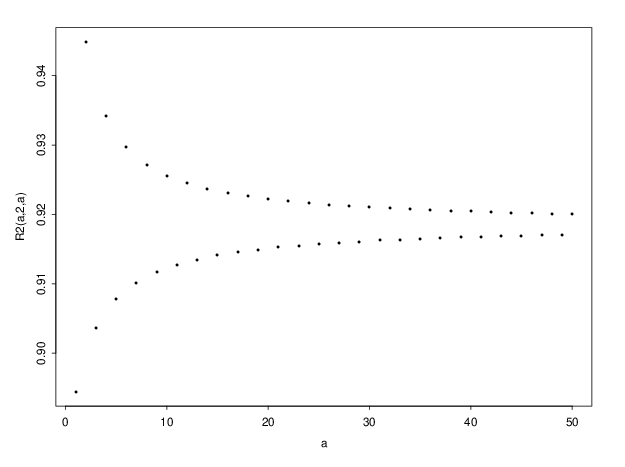
Exact formulae can be derived for R2​(a,2,a),a≥3R_{2}(a;2,a),\ a\geq 3. Indeed

(5.3) S2​(a,2,a)={a−12−⌊a/2⌋​(1+⌊a/2⌋)2​a if ​⌊a2⌋<a2, i.e., a is odd, a−12−14​(a2−1) if ​⌊a2⌋=a2, i.e., a is even. S_{2}(a;2,a)=\left\{\begin{array}[]{cl}\frac{a-1}{2}-\frac{\left\lfloor{a/2}\right\rfloor(1+\left\lfloor{a/2}\right\rfloor)}{2a}&\text{ if }\left\lfloor{\frac{a}{2}}\right\rfloor<\frac{a}{2},\text{ i.e., $a$ is odd, }\\ \frac{a-1}{2}-\frac{1}{4}\left(\frac{a}{2}-1\right)&\text{ if }\left\lfloor{\frac{a}{2}}\right\rfloor=\frac{a}{2},\text{ i.e., $a$ is even. }\end{array}\right.

Moreover

M2​(a,2)=1a​⌊a2⌋,M_{2}(a;2)=\frac{1}{a}\left\lfloor{\frac{a}{2}}\right\rfloor\ ,

and

M2​(a,a)=2​a2−3​a+16.M_{2}(a;a)=\frac{2a^{2}-3a+1}{6}\ .

Accordingly

(5.4) R2​(a,2,a)={R2∗​(a)​(a−1−1/a⁡⌊a/2⌋​(1+⌊a/2⌋)) if ​⌊a2⌋<a2, i.e., a is odd, R2∗​(a)​(a−1−1/2​(a/2−1)) if ​⌊a2⌋=a2, i.e., a is even, R_{2}(a;2,a)=\left\{\begin{array}[]{cl}R_{2}^{*}(a)\left(a-1-1/a\left\lfloor{a/2}\right\rfloor(1+\left\lfloor{a/2}\right\rfloor)\right)&\text{ if }\left\lfloor{\frac{a}{2}}\right\rfloor<\frac{a}{2},\text{ i.e., $a$ is odd, }\\ R_{2}^{*}(a)\left(a-1-1/2(a/2-1)\right)&\text{ if }\left\lfloor{\frac{a}{2}}\right\rfloor=\frac{a}{2},\text{ i.e., $a$ is even, }\end{array}\right.

where

(5.5) R2∗​(a)=6​a2​⌊a/2⌋​(2​a2−3​a+1).R_{2}^{*}(a)=\frac{\sqrt{6a}}{2\sqrt{\left\lfloor{a/2}\right\rfloor(2a^{2}-3a+1)}}\ .

A graph of R2​(a,2,a)R_{2}(a;2,a) for a=3,…,50a=3,\dots,50 is given in Figure 3. Notice that lima→∞R2​(a,2,a)=3​68\lim_{a\to\infty}R_{2}(a;2,a)=\frac{3\sqrt{6}}{8}.

Refer to caption
Figure 3. R2​(a,2,a)R_{2}(a;2,a) for a=3,…,50a=3,\dots,50

We provide here a few auxiliary results. First, if c=l+i​ac=l+ia (i.e., a≡lmodca\equiv l\mod c) then

(5.6) S2​(a,b,c)=∑m=0a−1⌊b​ma⌋​⌊(l+i​a)​ma⌋=i​∑m=1a−1m⁡⌊b​ma⌋+S2​(a,b,l).S_{2}(a;b,c)=\sum_{m=0}^{a-1}\left\lfloor{\frac{bm}{a}}\right\rfloor\left\lfloor{\frac{(l+ia)m}{a}}\right\rfloor=i\sum_{m=1}^{a-1}m\left\lfloor{\frac{bm}{a}}\right\rfloor+S_{2}(a;b,l)\ .

Similarly,

a​M2​(a,l+i​a)=∑m=0a−1⌊(l+i​a)​ma⌋2=i2​(a−1)​a​(2​a−1)6+2​i​∑m=1a−1m⁡⌊l​ma⌋+a​M2​(a,l).aM_{2}(a;l+ia)=\sum_{m=0}^{a-1}\left\lfloor{\frac{(l+ia)m}{a}}\right\rfloor^{2}=i^{2}\frac{(a-1)a(2a-1)}{6}+2i\sum_{m=1}^{a-1}m\left\lfloor{\frac{lm}{a}}\right\rfloor+aM_{2}(a,l)\ .

Accordingly,

(5.7) R2​(a,b,l+i​a)=i​∑m=1a−1m⁡⌊b​ma⌋+a​S2​(a,b,l)DiR_{2}(a;b,l+ia)=\frac{i\sum_{m=1}^{a-1}m\left\lfloor{\frac{bm}{a}}\right\rfloor+aS_{2}(a;b,l)}{D_{i}}

where

Di=i​(a​M2​(a,b)​(a−1)​a​(2​a−1)6+2i​∑m=1a−1m⁡⌊l​ma⌋+ai2​M2​(a,l))1/2.D_{i}=i\left(aM_{2}(a;b)\frac{(a-1)a(2a-1)}{6}+\frac{2}{i}\sum_{m=1}^{a-1}m\left\lfloor{\frac{lm}{a}}\right\rfloor+\frac{a}{i^{2}}M_{2}(a,l)\right)^{1/2}.

Thus,

limc→∞R2​(a,b,c)=limi→∞R2​(a,b,l+i​a)=R2​(a,b,a).\lim_{c\to\infty}R_{2}(a;b,c)=\lim_{i\to\infty}R_{2}(a;b,l+ia)=R_{2}(a;b,a)\ .

Now,

a​S2​(a,j​a,a)=∑m=0a−1⌊m​j​aa⌋​⌊m​aa⌋=j​∑m=0a−1m2=j​(a−1)​a​(2​a−1)6aS_{2}(a;ja,a)=\sum_{m=0}^{a-1}\left\lfloor{\frac{mja}{a}}\right\rfloor\left\lfloor{\frac{ma}{a}}\right\rfloor=j\sum_{m=0}^{a-1}m^{2}=j\frac{(a-1)a(2a-1)}{6}

and

a​M2​(a,j​a)=j2​∑m=0a−1m2=j2​(a−1)​a​(2​a−1)6,aM_{2}(a;ja)=j^{2}\sum_{m=0}^{a-1}m^{2}=j^{2}\frac{(a-1)a(2a-1)}{6}\ ,

whence

R2​(a,j​a,a)=1 for all ​j≥1.R_{2}(a;ja,a)=1\qquad\text{ for all }j\geq 1\ .

We consider now R2​(a,b,a)R_{2}(a;b,a) with a→∞a\to\infty. Let a=j​ba=jb. For j≥2j\geq 2

R2​(j​b,b,j​b)=∑m=jj​b−1m⁡⌊mj⌋(∑m=jj​b−1⌊mj⌋2​(a−1)​a​(2​a−1)6)1/2R_{2}(jb;b,jb)=\frac{\sum_{m=j}^{jb-1}m\left\lfloor{\frac{m}{j}}\right\rfloor}{\left(\sum_{m=j}^{jb-1}\left\lfloor{\frac{m}{j}}\right\rfloor^{2}\frac{(a-1)a(2a-1)}{6}\right)^{1/2}}
∑m=jj​b−1m⁡⌊mj⌋=∑l=1b−1l​∑m=l​j(l+1)​j−1m=b​j​(b−1)​(4​b​j+j−3)12\sum_{m=j}^{jb-1}m\left\lfloor{\frac{m}{j}}\right\rfloor=\sum_{l=1}^{b-1}l\sum_{m=lj}^{(l+1)j-1}m=\frac{bj(b-1)(4bj+j-3)}{12}
∑m=jj​b−1⌊mj⌋2=j​∑l=1b−1l2=j​(b−1)​b​(2​b−1)6.\sum_{m=j}^{jb-1}\left\lfloor{\frac{m}{j}}\right\rfloor^{2}=j\sum_{l=1}^{b-1}l^{2}=j\frac{(b-1)b(2b-1)}{6}\ .

Thus

(5.8) R2∗​(b)=limj→∞R2​(j​b,b,j​b)=limj→∞(b−1)​((4​b+1)​j−3)2​((b−1)​(2​b−1)​(j​b−1)​(2​j​b−1))1/2=2​(b−1)​(4​b+1)4​b​(b−1)​(2​b−1).R_{2}^{*}(b)=\lim_{j\to\infty}R_{2}(jb;b,jb)=\lim_{j\to\infty}\frac{(b-1)\left((4b+1)j-3\right)}{2\left((b-1)(2b-1)(jb-1)(2jb-1)\right)^{1/2}}=\frac{\sqrt{2}(b-1)(4b+1)}{4b\sqrt{(b-1)(2b-1)}}\ .

Some values of the limit are given in the table below.

bb R2∗​(b)R_{2}^{*}(b)
2 0.918558
3 0.96896
4 0.9836
Figure 4. Some values of R2∗​(b)=limj→∞R2​(j​b,b,j​b)R_{2}^{*}(b)=\lim_{j\to\infty}R_{2}(jb;b,jb)

5.2. A Geometric correspondence

We have seen that the Dedekind-like sums S2​(a,b,c)S_{2}(a;b,c) and M2​(a,b)M_{2}(a;b) can be considered as inner products in ℝa−1\mathbb{R}^{a-1}. Thus, for a given integer a≥3a\geq 3, we construct a polyhedral cone 𝒞a⊂ℝa−1\mathcal{C}_{a}\subset\mathbb{R}^{a-1} that is defined by the positive real span of the vectors

𝐯b=(⌊ba⌋,⌊2​ba⌋,…,⌊(a−1)​ba⌋), 1≤b<∞.{\bf v}_{b}=\left(\left\lfloor{\frac{b}{a}}\right\rfloor,\left\lfloor{\frac{2b}{a}}\right\rfloor,\dots,\left\lfloor{\frac{(a-1)b}{a}}\right\rfloor\right),\ 1\leq b<\infty.

As stated in the introduction, the significance of these vectors is that R2​(a,b,c)R_{2}(a;b,c) is the cosine of the angle between the two vectors 𝐯b{\bf v}_{b} and 𝐯c{\bf v}_{c}. The observation that R2​(a,b,c)R_{2}(a;b,c) is close to 11 is captured geometrically by the statement that this cone 𝒞a\mathcal{C}_{a} is thin in the angular metric.

Notice that 𝐯1=𝟎=(0,…,0){\bf v}_{1}={\bf 0}=(0,\dots,0) and 𝐯a=(1,2,…,a−1){\bf v}_{a}=(1,2,\dots,a-1). For b=2,3,…,a−1b=2,3,\dots,a-1, the vectors 𝐯b{\bf v}_{b} are

𝐯2=(0,…,0,1,…,1),𝐯3=(0,…,0,1,…,1,2,…,2),…,𝐯a−1=(0,1,…,a−2),{\bf v}_{2}=(0,\dots,0,1,\dots,1),{\bf v}_{3}=(0,\dots,0,1,\dots,1,2,\dots,2),\dots,{\bf v}_{a-1}=(0,1,\dots,a-2),

where each vector 𝐯j{\bf v}_{j} has almost equally distributed values for the integers the comprise its entries.

For b>ab>a, we write b=k​a+l,k>0, 0≤l<ab=ka+l,\ k>0,\ 0\leq l<a, and it follows from our notation that 𝐯b=k​𝐯a+𝐯l{\bf v}_{b}=k{\bf v}_{a}+{\bf v}_{l}. Thus the cone 𝒞a\mathcal{C}_{a} is in fact the positive real span of only the a−1a-1 vectors 𝐯b{\bf v}_{b} with b=2,3,…,ab=2,3,\dots,a.

Since 𝐯1=0{\bf v}_{1}=0, we have 𝐯k​a=𝐯k​a+1{\bf v}_{ka}={\bf v}_{ka+1}. Moreover, if Pl​(2≤l≤a−1)P_{l}\ (2\leq l\leq a-1) denotes the 2-dimensional plane containing the vectors 𝐯l{\bf v}_{l} and 𝐯a{\bf v}_{a}, then all the vectors 𝐯k​a+l,k=0,1,…{\bf v}_{ka+l},\ k=0,1,\dots belong to PlP_{l}. Notice that for different values of ll, say ll and l′≠ll^{\prime}\not=l, PlP_{l} and Pl′P_{l^{\prime}} are two different planes which have the ray

{r​𝐯a:r≥0}\left\{r\,{\bf v}_{a}:\ r\geq 0\right\}

in common (see Lemma 6). Throughout this section, the denominators in the vector components of all the vectors 𝐯m{\bf v}_{m} are always the integer aa.

Refer to caption
Figure 5. 𝐯a,𝐯b+k​𝐯a​(0≤k≤3),𝐯c+j​𝐯a​(0≤j≤3){\bf v}_{a},\ {\bf v}_{b}+k{\bf v}_{a}(0\leq k\leq 3),\ {\bf v}_{c}+j{\bf v}_{a}(0\leq j\leq 3)

The vectors 𝐯2,…,𝐯a{\bf v}_{2},\dots,{\bf v}_{a} are not always linearly independent. One can easily check that if a=3,4,6a=3,4,6 then these vectors are linearly independent, and when a=5,7,8,9,…a=5,7,8,9,\dots they are not. However, one can prove the following:

Lemma 6.

For each a≥4a\geq 4, the vectors 𝐯a,𝐯l,𝐯l′{\bf v}_{a},{\bf v}_{l},{\bf v}_{l^{\prime}}, where 1<l,l′<a1<l,l^{\prime}<a and l≠l′l\not=l^{\prime}, are linearly independent.

Proof. For each a≥4a\geq 4, 𝐯a=(1,2,…,a−1){\bf v}_{a}=(1,2,\dots,a-1), while the first component of both 𝐯l{\bf v}_{l} and 𝐯l′{\bf v}_{l^{\prime}} is zero; thus 𝐯a{\bf v}_{a} is linearly independent of {𝐯l,𝐯l′}\{{\bf v}_{l},{\bf v}_{l^{\prime}}\}. Moreover, 𝐯l{\bf v}_{l} and 𝐯l′{\bf v}_{l^{\prime}} do not lie on the same ray. □\Box

Lemma 7.

For each a≥3a\geq 3, if b1=k1​a+lb_{1}=k_{1}a+l and b2=k2​a+lb_{2}=k_{2}a+l, where 1≤k1<k21\leq k_{1}<k_{2}, then

R2​(a,l,a)<R2​(a,l,b2)<R2​(a,l,b1)R_{2}(a;l,a)<R_{2}(a;l,b_{2})<R_{2}(a;l,b_{1})

for all 1<l<a1<l<a.

Proof. The vectors 𝐯b1{\bf v}_{b_{1}} and 𝐯b2{\bf v}_{b_{2}} lie in PlP_{l}. Moreover, 𝐯b1=k1​𝐯a+𝐯l{\bf v}_{b_{1}}=k_{1}{\bf v}_{a}+{\bf v}_{l} and 𝐯b2=k2​𝐯a+𝐯l{\bf v}_{b_{2}}=k_{2}{\bf v}_{a}+{\bf v}_{l}. Hence

∠⁡(𝐯l,𝐯a)>∠⁡(𝐯b1,𝐯a)>∠⁡(𝐯b1,𝐯a).\angle\left({{\bf v}_{l},{\bf v}_{a}}\right)>\angle\left({{\bf v}_{b_{1}},{\bf v}_{a}}\right)>\angle\left({{\bf v}_{b_{1}},{\bf v}_{a}}\right)\ .

But ∠⁡(𝐯b,𝐯l)=∠⁡(𝐯a,𝐯l)−∠⁡(𝐯a,𝐯b)\angle\left({{\bf v}_{b},{\bf v}_{l}}\right)=\angle\left({{\bf v}_{a},{\bf v}_{l}}\right)-\angle\left({{\bf v}_{a},{\bf v}_{b}}\right), and the inequalites in the statement follow by taking cosines. □\Box

Notice that due to the monotonicity stated in the last lemma,

limk→∞R2​(a,l,k​a+l)=R2​(a,l,a).\lim_{k\to\infty}R_{2}(a;l,ka+l)=R_{2}(a;l,a)\ .

It is interesting to notice that in the case of a=3a=3, all vectors 𝐯b{\bf v}_{b} are between 𝐯2=(0,1){\bf v}_{2}=(0,1) and 𝐯3=(1,2){\bf v}_{3}=(1,2). The cosine of the angle between these two vectors is 2/52/\sqrt{5}.

Lemma 8.
  1. (i)

    If a=3,5a=3,5 then R2​(a,2,b)<R2​(a,3,b)R_{2}(a;2,b)<R_{2}(a;3,b) for all b≥3b\geq 3.

  2. (ii)

    If a=4a=4 then R2​(4,2,b)<R2​(4,3,b)R_{2}(4;2,b)<R_{2}(4;3,b) for all b≠6b\not=6. If b=6b=6 then R2​(4,2,6)=0.9708R_{2}(4;2,6)=0.9708 and R2​(4,3,6)=0.9647R_{2}(4;3,6)=0.9647.

Proof. (i) The case a=3a=3 follows immediately from Lemma 7. For a=5a=5 we have

𝐯2=(0,0,1,1),\displaystyle{\bf v}_{2}=(0,0,1,1), |𝐯2|=2\displaystyle\qquad|{\bf v}_{2}|=\sqrt{2}
𝐯3=(0,1,1,2),\displaystyle{\bf v}_{3}=(0,1,1,2), |𝐯3|=6\displaystyle\qquad|{\bf v}_{3}|=\sqrt{6}
𝐯4=(0,1,2,3),\displaystyle{\bf v}_{4}=(0,1,2,3), |𝐯4|=14\displaystyle\qquad|{\bf v}_{4}|=\sqrt{14}
𝐯5=(1,2,3,4),\displaystyle{\bf v}_{5}=(1,2,3,4), |𝐯5|=30.\displaystyle\qquad|{\bf v}_{5}|=\sqrt{30}\ .

Let (⋅,⋅)\left({\cdot},{\cdot}\right) denote the inner product of two vectors. For any b=5k+l,k=1,2,…,l=2,3,4b=5k+l,\ k=1,2,\dots,\ l=2,3,4,

R2​(5,2,5​k+l)<R2​(5,3,5​k+l)R_{2}(5;2,5k+l)<R_{2}(5;3,5k+l)

if and only if

12​(𝐯2,𝐯5​k+l)<16​(𝐯3,𝐯5​k+l).\frac{1}{\sqrt{2}}\left({{\bf v}_{2}},{{\bf v}_{5k+l}}\right)<\frac{1}{\sqrt{6}}\left({{\bf v}_{3}},{{\bf v}_{5k+l}}\right)\ .

This is equivalent to

6​k​(𝐯2,𝐯5)+6​(𝐯2,𝐯l)<2​k​(𝐯3,𝐯5)+2​(𝐯3,𝐯l),\sqrt{6}k\left({{\bf v}_{2}},{{\bf v}_{5}}\right)+\sqrt{6}\left({{\bf v}_{2}},{{\bf v}_{l}}\right)<\sqrt{2}k\left({{\bf v}_{3}},{{\bf v}_{5}}\right)+\sqrt{2}\left({{\bf v}_{3}},{{\bf v}_{l}}\right)\ ,

or

k⁡(13​2−7​6)>6​(𝐯2,𝐯l)−2​(𝐯3,𝐯l).k\left(13\sqrt{2}-7\sqrt{6}\right)>\sqrt{6}\left({{\bf v}_{2}},{{\bf v}_{l}}\right)-\sqrt{2}\left({{\bf v}_{3}},{{\bf v}_{l}}\right)\ .

Thus, for l=2l=2 the inequality is true for all k>0.53k>0.53; for l=3l=3 or 4 it is true for all k≥0k\geq 0. Notice that for l=2l=2 and k=0k=0, we get b=2b=2.

(ii) For a=4a=4, if b=4​k+2b=4k+2 then the inequality is true for all k>1.72k>1.72. For this reason, the inequality between R2​(4,2,6)R_{2}(4;2,6) and R2​(4,3,6)R_{2}(4;3,6) is reversed. If b=4​k+3b=4k+3 the inequality is true for all k≥0k\geq 0. □\Box

Empirical evidence suggests that R2​(a,2,b)<R2​(a,3,b)R_{2}(a;2,b)<R_{2}(a;3,b) for all a≥6a\geq 6 and b≥3b\geq 3. We do not give a formal proof.

Lemma 9.

For all a≥3a\geq 3, R2​(a,2,a)<R2​(a,3,a)R_{2}(a;2,a)<R_{2}(a;3,a).

Proof. If a=3a=3 then R2​(3,3,3)>R2​(3,2,3)R_{2}(3;3,3)>R_{2}(3;2,3). For all a≥4a\geq 4, we have to show that B⁡(a)>A⁡(a)B(a)>A(a), where

A⁡(a)=R2​(a,2,a)​|𝐯a| and B⁡(a)=R2​(a,3,a)​|𝐯a|.A(a)=R_{2}(a;2,a)|{\bf v}_{a}|\qquad\text{ and }\qquad B(a)=R_{2}(a;3,a)|{\bf v}_{a}|\ .

The formulas for A⁡(a),a≡0,1mod2A(a),\ a\equiv 0,1\mod 2 and B⁡(a),a≡0,1,2mod3B(a),\ a\equiv 0,1,2\mod 3 are given in Figure 6.

amod2a\mod 2 AA
0 2​a8​(3​a−2)\displaystyle\frac{\sqrt{2a}}{8}\,(3a-2)
1 12​⌊a/2⌋​(a+⌊a/2⌋)​(a−1−⌊a/2⌋)\displaystyle\frac{1}{2\sqrt{\left\lfloor{a/2}\right\rfloor}}\left(a+\left\lfloor{a/2}\right\rfloor\right)\left(a-1-\left\lfloor{a/2}\right\rfloor\right)
amod3a\mod 3 BB
0 15​a90​(13​a−9)\displaystyle\frac{\sqrt{15a}}{90}\,(13a-9)
1 a⁡(a−1)−3/2​⌊a/3⌋−5/2​⌊a/3⌋22​a−1−7/2​⌊a/3⌋\displaystyle\frac{a(a-1)-3/2\left\lfloor{a/3}\right\rfloor-5/2\left\lfloor{a/3}\right\rfloor^{2}}{2\sqrt{a-1-7/2\left\lfloor{a/3}\right\rfloor}}
2 a⁡(a−1)−1−7/2​⌊a/3⌋−5/2​⌊a/3⌋24​a+7−7​⌊a/3⌋\displaystyle\frac{a(a-1)-1-7/2\left\lfloor{a/3}\right\rfloor-5/2\left\lfloor{a/3}\right\rfloor^{2}}{\sqrt{4a+7-7\left\lfloor{a/3}\right\rfloor}}
Figure 6. A⁡(a),a≡0,1mod2A(a),\ a\equiv 0,1\mod 2 and B⁡(a),a≡0,1,2mod3B(a),\ a\equiv 0,1,2\mod 3

One can easily check in all six cases that B⁡(a)>A⁡(a)B(a)>A(a). □\Box

Lemma 10.

For each a≥3a\geq 3 and each b,c≥2b,c\geq 2

R2​(a,b,c)≥min⁡(R2​(a,l′,a),R2​(a,l,a),R2​(a,l′,l))R_{2}(a;b,c)\geq\min\left(R_{2}(a;l^{\prime},a),R_{2}(a;l,a),R_{2}(a;l^{\prime},l)\right)

where b≡lmoda,c≡l′modab\equiv l\mod a,\ c\equiv l^{\prime}\mod a.

Proof. If l,l′≡0,1modal,l^{\prime}\equiv 0,1\mod a, both 𝐯b{\bf v}_{b} and 𝐯c{\bf v}_{c} are on the ray RaR_{a}, and R2​(a,b,c)=1R_{2}(a;b,c)=1.

If l=l′=2,…,a−1l=l^{\prime}=2,\dots,a-1 then 𝐯b{\bf v}_{b} and 𝐯c{\bf v}_{c} belong to PlP_{l} and R2​(a,b,c)≥R2​(a,l,a)R_{2}(a;b,c)\geq R_{2}(a;l,a).

Finally, if l≠l′l\not=l^{\prime} one establishes the inequality by comparing the arcs on the unit sphere corresponding to the angles. These are the arcs between the points on the sphere on the rays generated by 𝐯a{\bf v}_{a}, 𝐯l{\bf v}_{l}, 𝐯l′{\bf v}_{l^{\prime}}, 𝐯b{\bf v}_{b}, and 𝐯c{\bf v}_{c}. □\Box

To prove Conjecture 1 it suffices to show that

mina≥3,b,c≥2⁡R2​(a,b,c)≥R2​(5,2,3).\min_{a\geq 3,\ b,c\geq 2}R_{2}(a;b,c)\geq R_{2}(5;2,3)\ .

Let R2∗​(a)=minb,c≥2⁡R2​(a,b,c)\displaystyle R_{2}^{*}(a)=\min_{b,c\geq 2}R_{2}(a;b,c). According to Lemma 10, for each a≥3a\geq 3

R2∗​(a)=min1<l,l′<a⁡min⁡(R2​(a,l′,a),R2​(a,l,a),R2​(a,l′,l)),R_{2}^{*}(a)=\min_{1<l,l^{\prime}<a}\min\left(R_{2}(a;l^{\prime},a),R_{2}(a;l,a),R_{2}(a;l^{\prime},l)\right)\ ,

whence

mina≥3,b,c≥2⁡R2​(a,b,c)=mina≥3⁡R2∗​(a).\min_{a\geq 3,\ b,c\geq 2}R_{2}(a;b,c)=\min_{a\geq 3}R_{2}^{*}(a)\ .

In Figure 7 we present a plot of R2∗​(a)R_{2}^{*}(a) for a=3,…,35a=3,\dots,35. We see that in this range, R2​(5,2,3)R_{2}(5;2,3) is the minimum, lending further credence to conjecture 1.

Refer to caption
Figure 7. R2∗​(a)R_{2}^{*}(a) for a=3,…,35a=3,\dots,35

6. Upper bounds for generalized Dedekind sums: higher dimensions

6.1. Probability models

We introduce now a probability space and random variables, whose (mixed) moments yield the SS- and MM-functions. Let 𝒟d(a)\mathcal{D}_{d}^{(a)} be a dd-dimensional discrete sample space, consisting of ada^{d} points, that is,

𝒟d(a)={(m1,…,md):mj=0,…,a−1,j=1,…,d}.\mathcal{D}_{d}^{(a)}=\left\{(m_{1},\dots,m_{d}):\ m_{j}=0,\dots,a-1,\ j=1,\dots,d\right\}.

A point in 𝒟d(a)\mathcal{D}_{d}^{(a)} is a dd-dimensional vector 𝐦=(m1,…,md){\bf m}=(m_{1},\dots,m_{d}). Consider the probability function on 𝒟d(a)\mathcal{D}_{d}^{(a)}:

(6.1) P⁡(𝐦)={1/a if 𝐦=j𝟏d,j=0,…,a−10 otherwise, P({\bf m})=\left\{\begin{array}[]{cl}1/a&\text{ if }{\bf m}=j{\bf 1}_{d},\ j=0,\dots,a-1\\ 0&\text{ otherwise, }\end{array}\right.

where 𝟏d=(1,1,1,…,1){\bf 1}_{d}=(1,1,1,\dots,1). This probability function is concentrated on the main diagonal points of 𝒟d(a)\mathcal{D}_{d}^{(a)}. Define the random variables

(6.2) Xi(a)​(𝐦,𝐛)={⌊m​bia⌋ if 𝐦=m𝟏d,m=0,…,a−1,0 otherwise, X_{i}^{(a)}({\bf m};{\bf b})=\left\{\begin{array}[]{cl}\left\lfloor{\frac{mb_{i}}{a}}\right\rfloor&\text{ if }{\bf m}=m{\bf 1}_{d},\ m=0,\dots,a-1,\\ 0&\text{ otherwise, }\end{array}\right.

where 𝐛=(b1,…,bd){\bf b}=(b_{1},\dots,b_{d}). It follows immediately that

(6.3) Sd​(a,𝐛)=EP​{∏i=1dXi(a)​(𝐦,𝐛)},S_{d}(a;{\bf b})=E_{P}\left\{\prod_{i=1}^{d}X_{i}^{(a)}({\bf m};{\bf b})\right\},

where EP​{}E_{P}\{\ \} denotes the expected value of the term in braces with respect to the probability function PP. Moreover,

(6.4) Mk​(a,bi)=EP​{(Xi(a)​(𝐦,𝐛))k}.M_{k}(a;b_{i})=E_{P}\left\{\left(X_{i}^{(a)}({\bf m};{\bf b})\right)^{k}\right\}.

Notice that Mk​(a,bi)M_{k}(a;b_{i}) is the kk-th order moment of Xi(a)​(𝐦,𝐛)X_{i}^{(a)}({\bf m};{\bf b}). The Dilcher-Girstmair presentation of the SS- and MM-functions can be described as moments of the random variables

(6.5) Ji(a)(𝐦;𝐛)=∑j=0bi−1jI{𝐦:j​abi≤mi<(j+1)​abi},i=1,…,d,J_{i}^{(a)}({\bf m};{\bf b})=\sum_{j=0}^{b_{i}-1}j\,I\left\{{\bf m}:\ \frac{ja}{b_{i}}\leq m_{i}<\frac{(j+1)a}{b_{i}}\right\},\ i=1,\dots,d,

where I​{𝐦:…}I\{{\bf m}:\dots\} is the indicator function. According to this definition,

(6.6) Sd​(a,𝐛)=EP​{∏i=1dJi(a)​(𝐦,𝐛)}S_{d}(a;{\bf b})=E_{P}\left\{\prod_{i=1}^{d}J_{i}^{(a)}({\bf m};{\bf b})\right\}

and

(6.7) Mk​(a,bi)=EP​{(Ji(a)​(𝐦,𝐛))k}.M_{k}(a;b_{i})=E_{P}\left\{\left(J_{i}^{(a)}({\bf m};{\bf b})\right)^{k}\right\}.

6.2. Upper bounds for Sd​(a,𝐛)S_{d}(a;{\bf b})

In the present section we use the random variables Xi(a)​(𝐦,𝐛)X_{i}^{(a)}({\bf m};{\bf b}). Since aa and 𝐛{\bf b} are fixed, we will simplify the notation to calling the random variables X1,…,XdX_{1},\dots,X_{d}. Repeated application of the Cauchy-Schwartz inequality yields bounds in terms of the one-dimensional moments MM. For example, for d=2d=2 we obtain

E⁡{X1​X2}≤(E⁡{X12}​E​{X22})1/2,E\left\{X_{1}X_{2}\right\}\leq\left(E\left\{X_{1}^{2}\right\}E\left\{X_{2}^{2}\right\}\right)^{1/2},

and thus

S2​(a,b1,b2)≤(M2​(a,b1)​M2​(a,b2))1/2.S_{2}(a;b_{1},b_{2})\leq\left(M_{2}(a,b_{1})M_{2}(a,b_{2})\right)^{1/2}.

For d=3d=3 we get

E⁡{X1​X2​X3}≤(E⁡{X12}​E​{X22​X32})1/2≤(E⁡{X12}​(E⁡{X24}​E​{X34})1/2)1/2E\left\{X_{1}X_{2}X_{3}\right\}\leq\left(E\left\{X_{1}^{2}\right\}E\left\{X_{2}^{2}X_{3}^{2}\right\}\right)^{1/2}\leq\left(E\left\{X_{1}^{2}\right\}\left(E\left\{X_{2}^{4}\right\}E\left\{X_{3}^{4}\right\}\right)^{1/2}\right)^{1/2}

or

(6.8) S3​(a,b1,b2,b3)≤M21/2​(a,b1)​M41/4​(a,b2)​M41/4​(a,b3).S_{3}(a;b_{1},b_{2},b_{3})\leq M_{2}^{1/2}(a,b_{1})M_{4}^{1/4}(a,b_{2})M_{4}^{1/4}(a,b_{3})\ .

By taking the geometric mean of the cyclical permutations, we get the symmetric upper bound

S3​(a,b1,b2,b3)≤(∏j=13M2​(a,bj)​M4​(a,bj))1/6.S_{3}(a;b_{1},b_{2},b_{3})\leq\left(\prod_{j=1}^{3}M_{2}(a,b_{j})M_{4}(a,b_{j})\right)^{1/6}\ .

For d=4d=4 we similarly obtain

(6.9) S4​(a,b1,b2,b3,b4)≤(∏j=14M4​(a,bj))1/4.S_{4}(a;b_{1},b_{2},b_{3},b_{4})\leq\left(\prod_{j=1}^{4}M_{4}(a,b_{j})\right)^{1/4}\ .

For d=5d=5 we start with

S5​(a,𝐛)\displaystyle S_{5}(a;{\bf b}) =EP{X1⋯X5}\displaystyle=E_{P}\left\{X_{1}\cdots X_{5}\right\}
≤(EP​{X12​X22})1/2​(EP​{X32​X42​X52})1/2\displaystyle\leq\left(E_{P}\left\{X_{1}^{2}X_{2}^{2}\right\}\right)^{1/2}\left(E_{P}\left\{X_{3}^{2}X_{4}^{2}X_{5}^{2}\right\}\right)^{1/2}
≤(M4​(a,b1)​M4​(a,b2))1/4​(∏j=35M4​(a,bj)​M8​(a,bj))1/12\displaystyle\leq\left(M_{4}(a;b_{1})M_{4}(a;b_{2})\right)^{1/4}\left(\prod_{j=3}^{5}M_{4}(a;b_{j})M_{8}(a;b_{j})\right)^{1/12}

Symmetrizing this upper bound by taking the geometric mean of the (52)\binom{5}{2} different bounds obtained by different selections of pairs and triplets gives

(6.10) S5​(a,𝐛)≤(∏j=15M43​(a,bj)​M8​(a,bj))1/20.S_{5}(a;{\bf b})\leq\left(\prod_{j=1}^{5}M_{4}^{3}(a;b_{j})M_{8}(a;b_{j})\right)^{1/20}.

From the upper bound for S3S_{3} we immediately obtain

(6.11) S6​(a,𝐛)≤(∏j=16M4​(a,bj)​M8​(a,bj))1/12.S_{6}(a;{\bf b})\leq\left(\prod_{j=1}^{6}M_{4}(a;b_{j})M_{8}(a;b_{j})\right)^{1/12}.

Generally, if d=2k,k=1,2,…d=2k,\ k=1,2,\dots, we have

(6.12) S2​k(a;𝐛)≤(EP{X12⋯Xk2})1/2(EP{Xk+12⋯X2​k2})1/2,S_{2k}(a;{\bf b})\leq\left(E_{P}\left\{X_{1}^{2}\cdots X_{k}^{2}\right\}\right)^{1/2}\left(E_{P}\left\{X_{k+1}^{2}\cdots X_{2k}^{2}\right\}\right)^{1/2},

from which we get, by utilizing previous results, symmetric upper bounds. For example,

(6.13) S8​(a,𝐛)\displaystyle S_{8}(a;{\bf b}) ≤(M8(a;b1)⋯M8(a;b4))1/8(M8(a;b5)⋯M8(a;b8))1/8\displaystyle\leq\left(M_{8}(a;b_{1})\cdots M_{8}(a;b_{4})\right)^{1/8}\left(M_{8}(a;b_{5})\cdots M_{8}(a;b_{8})\right)^{1/8}
=(M8(a;b1)⋯M8(a;b8))1/8,\displaystyle=\left(M_{8}(a;b_{1})\cdots M_{8}(a;b_{8})\right)^{1/8},

and

(6.14) S10​(a,𝐛)≤(∏j=110M83​(a,bj)​M16​(a,bj))1/40.S_{10}(a;{\bf b})\leq\left(\prod_{j=1}^{10}M_{8}^{3}(a;b_{j})M_{16}(a;b_{j})\right)^{1/40}.

We can immediately prove by induction the following:

Lemma 11.
(6.15) S2k(a;𝐛)≤(∏j=12kM2k(a;bj))1/2k,k=1,2,…S_{2^{k}}(a;{\bf b})\leq\left(\prod_{j=1}^{2^{k}}M_{2^{k}}(a;b_{j})\right)^{1/2^{k}},\ k=1,2,\dots

Similarly, for k=0,1,…k=0,1,\dots

(6.16) S3⋅2k​(a,𝐛)≤(∏j=13⋅2kM2k+1​(a,bj)​M2k+2​(a,bj))1/6⋅2kS_{3\cdot 2^{k}}(a;{\bf b})\leq\left(\prod_{j=1}^{3\cdot 2^{k}}M_{2^{k+1}}(a;b_{j})M_{2^{k+2}}(a;b_{j})\right)^{1/6\cdot 2^{k}}

and

(6.17) S5⋅2k​(a,𝐛)≤(∏j=15⋅2kM2k+23​(a,bj)​M2k+3​(a,bj))1/20⋅2k.S_{5\cdot 2^{k}}(a;{\bf b})\leq\left(\prod_{j=1}^{5\cdot 2^{k}}M_{2^{k+2}}^{3}(a;b_{j})M_{2^{k+3}}(a;b_{j})\right)^{1/20\cdot 2^{k}}.

If d=2​k+1d=2k+1 one needs a two-stage process of first partitioning to

(EP​{∏j=1kXj2})1/2​(EP​{∏j=1k+1Xk+j2})1/2\left(E_{P}\left\{\prod_{j=1}^{k}X_{j}^{2}\right\}\right)^{1/2}\left(E_{P}\left\{\prod_{j=1}^{k+1}X_{k+j}^{2}\right\}\right)^{1/2}

and then symmetrizing.

Before concluding this section, we remark that the above upper bounds for the SS-functions are generally not unique. By different partitions one can obtain different bounds. For example, in the case of S5S_{5}, one could start with

EP{X1⋯X5}≤(EP{X12})1/2(EP{X22⋯X52})1/2=(M2(a;b1))1/2(∏j=25M8(a;bj))1/8.E_{P}\left\{X_{1}\cdots X_{5}\right\}\leq\left(E_{P}\left\{X_{1}^{2}\right\}\right)^{1/2}\left(E_{P}\left\{X_{2}^{2}\cdots X_{5}^{2}\right\}\right)^{1/2}=\left(M_{2}(a;b_{1})\right)^{1/2}\left(\prod_{j=2}^{5}M_{8}(a;b_{j})\right)^{1/8}.

After symmetrization we get

(6.18) S5​(a,𝐛)≤(∏j=15M2​(a,bj)​M8​(a,bj))1/10.S_{5}(a;{\bf b})\leq\left(\prod_{j=1}^{5}M_{2}(a;b_{j})M_{8}(a;b_{j})\right)^{1/10}.

The question is which upper bound should be used, (6.10) or (6.18)? For example, if a=31a=31 and 𝐛=(3,5,7,11,13){\bf b}=(3,5,7,11,13) then S5​(a,𝐛)=1213.806S_{5}(a;{\bf b})=1213.806. The upper bound given by (6.10) is 1321.3211321.321, whereas that given by (6.18) is 1456.9851456.985. In the following table we present some exact values of S5​(a,𝐛)S_{5}(a;{\bf b}) and the two bounds (6.10) and (6.18). We also show R5​(a,𝐛)R_{5}(a;{\bf b}), the ratio of S5​(a,𝐛)S_{5}(a;{\bf b}) to the upper bound (6.10).

aa 𝐛{\bf b} S5S_{5} bound (6.10) bound (6.18) R5R_{5}
31 (3, 5, 7, 11, 13) 1213.806 1321.321 1456.985 0.9186
21 (5, 7, 9, 11, 13) 4411.333 4668.719 5190.201 0.9449
23 (5, 9, 11, 13, 17) 11429.74 12050.58 13385.72 0.9485
27 (5, 11, 13, 17, 21) 28101.93 29617.94 33011.8 0.9488
33 (7, 11, 13, 19, 23) 51943.76 54384.26 60525.59 0.9551
Figure 8. Some values and bounds of S5S_{5}

It seems from Figure 8 that the upper bound given by (6.10) is closer to the exact value of S5​(a,𝐛)S_{5}(a;{\bf b}) than (6.18). It is the preferred upper bound. It is also interesting that, like in the case of R2​(a,𝐛)R_{2}(a;{\bf b}), all values of R5​(a,𝐛)R_{5}(a;{\bf b}) in Figure 8 are greater than 0.91860.9186.

6.3. Relationships to upper bounds revisited

We study now upper bounds to SdS_{d} of the type given by (6.8)–(6.17). In particular, define

(6.19) R3​(a,𝐛)\displaystyle R_{3}(a;{\bf b}) =S3​(a,𝐛)(∏j=13M2​(a,bj)​M4​(a,bj))1/6,\displaystyle=\frac{S_{3}(a;{\bf b})}{\left(\prod_{j=1}^{3}M_{2}(a,b_{j})M_{4}(a,b_{j})\right)^{1/6}}\ ,
(6.20) R4​(a,𝐛)\displaystyle R_{4}(a;{\bf b}) =S4​(a,𝐛)(∏j=14M4​(a,bj))1/4, and\displaystyle=\frac{S_{4}(a;{\bf b})}{\left(\prod_{j=1}^{4}M_{4}(a,b_{j})\right)^{1/4}}\ ,\text{ and }
(6.21) R5​(a,𝐛)\displaystyle R_{5}(a;{\bf b}) =S5​(a,𝐛)(∏j=15M43​(a,bj)​M8​(a,bj))1/20.\displaystyle=\frac{S_{5}(a;{\bf b})}{\left(\prod_{j=1}^{5}M_{4}^{3}(a;b_{j})M_{8}(a;b_{j})\right)^{1/20}}\ .

A few values of R5​(a,𝐛)R_{5}(a;{\bf b}) are given in in Figure 8. It seems that the minimal R5​(a,𝐛)R_{5}(a;{\bf b}) value is R5​(7,2,3,4,5,6)=0.8567R_{5}(7;2,3,4,5,6)=0.8567. It is also interesting to observe that R5R_{5}, as shown in Figure 8, is generally above 0.90.9, as in the case of R2R_{2}, despite the increase in dimension from 2 to 5. We try to explain this phenomenon in probability terms.

As shown in (6.3) and (6.6),

Sd(a;𝐛)=EP{X1⋯Xd}=EP{J1⋯Jd}.S_{d}(a;{\bf b})=E_{P}\left\{X_{1}\cdots X_{d}\right\}=E_{P}\left\{J_{1}\cdots J_{d}\right\}\ .

Consider the case d=2d=2. According to the law of iterated expectation [1],

(6.22) S2​(a,b1,b2)=EP​{J(a)​(𝐦,b1)​EP​{J(a)​(𝐦,b2)∣J(a)​(𝐦,b1)}},S_{2}(a;b_{1},b_{2})=E_{P}\left\{J^{(a)}({\bf m};b_{1})E_{P}\left\{J^{(a)}({\bf m};b_{2})\mid J^{(a)}({\bf m};b_{1})\right\}\right\}\ ,

where the second term on the right-hand side is the conditional expectation of J(a)​(𝐦,b2)J^{(a)}({\bf m};b_{2}), given J(a)​(𝐦,b1)J^{(a)}({\bf m};b_{1}). Notice that in the notation of Section 3,

(6.23) S2​(a,b,c)=1a​∑j=0b−1∑l=0c−1j​l​fa;b,c​(j,l)=1a​∑j=0b−1j​fa;b​(j)​∑l=0c−1l​fa;b,c​(j,l)fa;b​(j).S_{2}(a;b,c)=\frac{1}{a}\sum_{j=0}^{b-1}\sum_{l=0}^{c-1}jlf_{a;b,c}(j,l)=\frac{1}{a}\sum_{j=0}^{b-1}jf_{a;b}(j)\sum_{l=0}^{c-1}l\frac{f_{a;b,c}(j,l)}{f_{a;b}(j)}\ .

The key to understanding the phenomenon is that the joint frequencies fa;b,c​(j,l)f_{a;b,c}(j,l) are distributed along the main diagonal, as illustrated in Figure 2. In the special case that b=cb=c,

fa;b,c​(j,l)={fa;b​(j)=fa;c​(j) if ​j≠l,0 otherwise. f_{a;b,c}(j,l)=\left\{\begin{array}[]{cl}f_{a;b}(j)=f_{a;c}(j)&\text{ if }j\not=l,\\ 0&\text{ otherwise. }\end{array}\right.

In this case,

∑l=0b−1l​fa;b,c​(j,l)fa;b​(j)=j\sum_{l=0}^{b-1}l\frac{f_{a;b,c}(j,l)}{f_{a;b}(j)}=j

and

S2​(a,b,b)=1a​∑j=0b−1j2​fa;b​(j)=M2​(a,b),S_{2}(a;b,b)=\frac{1}{a}\sum_{j=0}^{b-1}j^{2}f_{a;b}(j)=M_{2}(a;b)\ ,

as expected. When b≠cb\not=c then R2R_{2} is always smaller than 1, but might be quite close to it, even when bb and cc are different. For example, R2​(50,7,13)=0.9955R_{2}(50;7,13)=0.9955.

6.4. One-dimensional moments relationships

We present here some inequalities between Mr​(a,b)M_{r}(a;b) for fixed values of aa and bb and for variable rr.

Theorem 12.

Mr​(a,b)M_{r}(a;b) is log-convex in rr. That is,

(6.24) M2​r​(a,b)​M2​r+2​(a,b)−M2​r+12​(a,b)>0.M_{2r}(a;b)M_{2r+2}(a;b)-M_{2r+1}^{2}(a;b)>0.

Proof. First, by Liapounov’s inequality of moments [6, p. 627] we have

M1<M21/2<M31/3<…M_{1}<M_{2}^{1/2}<M_{3}^{1/3}<\dots

By factoring ⌊…⌋2​r+1=⌊…⌋r​⌊…⌋r+1\left\lfloor\dots\right\rfloor^{2r+1}=\left\lfloor\dots\right\rfloor^{r}\left\lfloor\dots\right\rfloor^{r+1} we obtain the inequality

(6.25) M2​r+12​(a,b)<M2​r​(a,b)​M2​r+2​(a,b)M_{2r+1}^{2}(a;b)<M_{2r}(a;b)M_{2r+2}(a;b)

for all r≥1r\geq 1. That is, Mr​(a,b)M_{r}(a;b) is log-convex in rr. □\Box

Appendix

Algorithm for Determining fba​(i),i=0,…,b−1f_{b}^{a}(i),\ i=0,\dots,b-1

STEP 0:
Set:
    (i) r = a/b;
    (ii) l = a-b*[r];
    (iii) f = 0(1,b);         # b-dimensional vector of zeros

STEP 1:

Compute:
    f [0] <- 1+[r];
    f [ i ] <- [(i+1)*r]- [i*r], i=1,..,(b-2);
    f [ b-1] <- a-1- [(b-1)*r];

STEP 2:

    IF((l=0) or (b=2)) { GOTO STEP 3 };
    ELSE {
        FOR ( i=1,...,b-2) {
            IF( [(i+1)*r] = r*(i+1) ) {
                f[i] <- f[i]-1;
                f[i+1] <- f[i+1]+1;
            }
        }

STEP 3:

PRINT f

END.

Algorithm for Determining fb​ca​(i,j)f_{bc}^{a}(i,j)

STEP 0:

Set:
    r1 <- a/b;
    r2 <- a/c;
    l1 <- a -b*[r1];
    l2 <- a - c*[r2];
    CT <- O((b+1),(c+1));    # matrix of zeros, of dimensions (b+1)*(c+1)
    t1 <- O(b,1);
    t2 <- O(1,c);

STEP 1:

Compute:
    CT[i,(c+1)] <- f_b[i-1], i=1,...,b;
    CT[(b+1), j] <- f_c[j-1], j=1,...,c;
    CT[(b+1),(c+1)] <- a;
    CT[1,1] <- min( CT[1,c+1], CT[b+1,1]);
    t2[1] <- t2[1] + CT[1,1];

STEP 2:

Compute:
    FOR (i=2,...,b) {
    CT[i,1] <- max(0, min(f_c[1]-t2[1], f_b[i-1])));
    t2[1] <- t2[1] + CT[i,1];
    }
    t1 <- CT[1:b,1];

STEP 3:

Compute:
    FOR (j=2,...,c) {
    CT[1,j] <- max(0,min(f_b[0]-t1[1], f_c[j-1]));
    t1[1] <- t1[1] + CT[1,j];
    t2[j] <- t2[j] + CT[1,j];
    }

STEP 4:

Compute:
    FOR (i=2,...,b) {
        FOR(j=2,...,c) {
        cty<- max(0, min(f_b[i-1]- t1[i], f_c[j-1]));
        ctx <- max(0, min(f_c[j-1]-t2[j], f_b[i-1]));
        CT[i,j] <- min(ctx,cty)
        t1[ i ] <- t1 [ i ]+  CT [ i, j];
        t2[ j ] <- t2 [ j ] + CT [i , j];
        }
    }

STEP 5:
Print CT

END.

References

  • [1] Peter J. Bickel and Kjell A. Doksum, Mathematical statistics, Holden-Day Inc., San Francisco, Calif., 1976, Basic ideas and selected topics, Holden-Day Series in Probability and Statistics. MR 56 #1513
  • [2] R. Dedekind, Erläuterungen zu den Fragmenten xxviii, Collected works of Bernhard Riemann, Dover Publ., New York, 1953, pp. 466–478.
  • [3] Karl Dilcher and Kurt Girstmair, Dedekind sums and uniform distributions, Amer. Math. Monthly 109 (2002), no. 3, 279–284.
  • [4] F. Hirzebruch and D. Zagier, The Atiyah-Singer theorem and elementary number theory, Publish or Perish Inc., Boston, Mass., 1974, Mathematics Lecture Series, No. 3. MR 58 #31291
  • [5] Donald E. Knuth, The art of computer programming. Vol. 2, second ed., Addison-Wesley Publishing Co., Reading, Mass., 1981, Seminumerical algorithms, Addison-Wesley Series in Computer Science and Information Processing. MR 83i:68003
  • [6] Samuel Kotz, Norman L. Johnson, and Campbell B. Read (eds.), Encyclopedia of statistical sciences. Vol. 4, John Wiley & Sons Inc., New York, 1983, Icing the tails to Limit theorems, Lecture Notes in Economics and Mathematical Systems, 192. MR 84k:62001b
  • [7] C. Meyer, Über einige Anwendungen Dedekindscher Summen, J. Reine Angew. Math. 198 (1957), 143–203. MR 21 #3396
  • [8] L. J. Mordell, Lattice points in a tetrahedron and generalized Dedekind sums, J. Indian Math. Soc. (N.S.) 15 (1951), 41–46. MR 13,322b
  • [9] Hans Rademacher and Emil Grosswald, Dedekind sums, The Mathematical Association of America, Washington, D.C., 1972, The Carus Mathematical Monographs, No. 16. MR 50 #9767