The displacement map associated to polynomial unfoldings of planar Hamiltonian vector fields

Lubomir Gavrilov Affiliation: Laboratoire Emile Picard, CNRS UMR 5580, Université Paul Sabatier Affiliation: 118, route de Narbonne, 31062 Toulouse Cedex, France Affiliation: Iliya D. Iliev Affiliation: Institute of Mathematics, Bulgarian Academy of Sciences Affiliation: Acad. G. Bonchev Str, Bldg 8, 1113 Sofia, Bulgaria

September 10, 2004

Abstract

We study the displacement map associated to small one-parameter polynomial unfoldings of polynomial Hamiltonian vector fields on the plane. Its leading term, the generating function $M(t)$ , has an analytic continuation in the complex plane and the real zeroes of $M(t)$ correspond to the limit cycles bifurcating from the periodic orbits of the Hamiltonian flow. We give a geometric description of the monodromy group of $M(t)$ and use it to formulate sufficient conditions for $M(t)$ to satisfy a differential equation of Fuchs or Picard-Fuchs type. As examples, we consider in more detail the Hamiltonian vector fields $\dot{z}=i\bar{z}-i(z+\bar{z})^{3}$ and $\dot{z}=iz+\bar{z}^{2}$ , possessing a rotational symmetry of order two and three, respectively. In both cases $M(t)$ satisfies a Fuchs-type equation but in the first example $M(t)$ is always an Abelian integral (that is to say, the corresponding equation is of Picard-Fuchs type) while in the second one this is not necessarily true. We derive an explicit formula of $M(t)$ and estimate the number of its real zeroes.

1 Introduction

Consider a perturbed planar Hamiltonian vector field

\left\{\begin{array}[]{l}\dot{x}=H_{y}(x,y)+\varepsilon P(x,y,\varepsilon),\\ \dot{y}=-H_{x}(x,y)+\varepsilon Q(x,y,\varepsilon).\end{array}\right.

(1_{ε})

We suppose that $H,P,Q$ are real polynomials in $x,y$ and moreover, $P,Q$ depend analytically on a small real parameter $\varepsilon$ . Assume that for a certain open interval $\Sigma\subset\mbox{\of R}$ , the level sets of the Hamiltonian $\{H=t\}$ , $t\in\Sigma$ , contain a continuous in $t$ family of ovals $\cal A$ . (An oval is a smooth simple closed curve which is free of critical points of $H$ ). Such a family is called a period annulus of the unperturbed system $(1_{0})$ . Typically, the endpoints of $\Sigma$ are critical levels of the Hamiltonian function that correspond to centers, saddle-loops or infinity. The limit cycles (that is, the isolated periodic trajectories) of $(1_{\varepsilon})$ which tend to ovals from $\cal A$ as $\varepsilon\to 0$ correspond to the zeros of the displacement map ${\cal P}_{\varepsilon}(t)-t$ , where the first return map ${\cal P}_{\varepsilon}(t)$ is defined on Fig. 1. More explicitly, take a segment $\sigma$ which is transversal to the family of ovals $\cal A$ and parameterize it by using the Hamiltonian value $t$ . For small $\varepsilon$ , $\sigma$ remains transversal to the flow of $(1_{\varepsilon})$ , too. Take a point $S\in\sigma$ and let $t=H(S)$ . The trajectory of $(1_{\varepsilon})$ through $S$ , after making one round, will intersect $\sigma$ again at some point $S_{1}$ and the first return map ${\cal P}_{\varepsilon}(t)$ is then defined by $t\rightarrow H(S_{1})$ .

Fixing a period annulus $\cal A$ of $(1_{0})$ and taking a nonintegrable deformation $(1_{\varepsilon})$ , then the related displacement map is defined in the corresponding open interval $\Sigma\subset\mbox{\of R}$ and there is a natural number $k$ so that

{\cal P}_{\varepsilon}(t)-t=M(t)\varepsilon^{k}+...,\quad t\in\Sigma.

(2_{k})

The limit cycles of $(1_{\varepsilon})$ which tend to periodic orbits from $\cal A$ as $\varepsilon\to 0$ correspond therefore to the zeros of the generating function $M(t)$ in $\Sigma$ .

The goal of the paper is to study the analytic continuation of the generating function $M(t)$ in a complex domain. We give a geometric description of the monodromy group of $M(t)$ (Theorem 1) from which we deduce sufficient conditions for $M(t)$ to satisfy a differential equation of Fuchs or Picard-Fuchs type (Theorem 2).

Recall that a Fuchsian equation is said to be of Picard-Fuchs type, provided that it possesses a fundamental set of solutions which are Abelian integrals (depending on a parameter). In the present paper by an Abelian integral we mean a function of the form

I(t)=\int_{\delta(t)}\omega

(3)

where

•

$\omega$ is a rational one-form in $\mbox{\of C}^{2}$ ;
•

there exists a bivariate polynomial $f:\mbox{\of C}^{2}\rightarrow\mbox{\of C}$ such that $\delta(t)\subset f^{-1}(t)$ , where $\{\delta(t)\}$ is a family of closed loops, depending continuously on the complex parameter $t$ .

It is supposed that $t$ belongs to some simply connected open subset of ℂ and $\delta(t)$ avoids the possible singularities of the one-form $\omega$ restricted to the level sets $f^{-1}(t)$ . Under these conditions $I(t)$ satisfies a linear differential equation of Fuchs, and hence of Picard-Fuchs type.

It is well known that for a generic perturbation in $(1_{\varepsilon})$ one has $k=1$ in $(2_{k})$ and moreover,

M(t)=\int_{\delta(t)}Q(x,y,0)dx-P(x,y,0)dy,\quad t\in\Sigma

is then an Abelian integral [19]. Here $\delta(t)\subset\mbox{\of R}^{2}$ , ${\cal A}=\{\delta(t)\}$ , $t\in\Sigma$ , is the continuous family of ovals defined by the polynomial $H(x,y)$ and the monodromy of $M(t)$ is deduced from the monodromy of $\delta(t)$ in a complex domain. More precisely, let $\Delta$ be the finite set of atypical values of $H:\mbox{\of C}^{2}\rightarrow\mbox{\of C}$ . The homology bundle associated to the polynomial fibration

\mbox{\of C}^{2}\setminus H^{-1}(\Delta)\stackrel{{\scriptstyle H}}{{\rightarrow}}\mbox{\of C}\setminus\Delta

has a canonical connection. The monodromy group of the Abelian integral $M(t)$ is then the monodromy group of the connection (or a subgroup of it). It is clear that $M(t)$ depends on the homology class of $\delta(t)$ in $H_{1}(\Gamma_{t},\mbox{\of Z})$ where $\Gamma_{t}$ is the algebraic curve $\{(x,y)\in\mbox{\of C}^{2}:H(x,y)=t\}$ .

On the other hand, there are perturbations $(1_{\varepsilon})$ with $k>1$ in $(2_{k})$ . This happens when the perturbation is so chosen that the first several coefficients in the expansion of the displacement map, among them the function $M(t)$ given by the above explicit integral, are identically zero in $\Sigma$ . One needs to consider such perturbations in order to set a proper bound on the number of bifurcating limit cycles e.g. when the Hamiltonian possesses symmetry or the degree of the perturbation is greater than the degree of the original system. Therefore, the case when $k>1$ is the more interesting one, at least what concerns the infinitesimal Hilbert’s 16th problem which is to find the maximal number of limit cycles in $(1_{\varepsilon})$ , in terms of the degrees of $H,P,Q$ only. In this case the generating function $M(t)$ can have more zeroes in $\Sigma$ , and respectively the perturbations with $k>1$ can produce in general more limit cycles than the ones with $k=1$ (see e.g. [9], [11], [6] for examples). Moreover, this case is more difficult because the generating function is not necessarily an Abelian integral and even the calculation of $M(t)$ itself is a challenging problem. It turns out that in general (when $k>1$ ), the generating function $M(t)$ depends on the free homotopy class of the closed loop $\delta(t)\subset\Gamma_{t}$ (Proposition 1). The homology group $H_{1}(\Gamma_{t},\mbox{\of Z})$ must be replaced in this case by another Abelian group $H_{1}^{\delta}(\Gamma_{t},\mbox{\of Z})$ which we define in section 2.2. Although there is a canonical homomorphism

H_{1}^{\delta}(\Gamma_{t},\mbox{\of Z})\rightarrow H_{1}(\Gamma_{t},\mbox{\of Z})

it is neither surjective, nor injective in general. The bundle associated to $H_{1}^{\delta}(\Gamma_{t},\mbox{\of Z})$ has a canonical connection too and this is the appropriate framework for the study of $M(t)$ . This construction might be of independent interest in the topological study of polynomial fibrations.

To illustrate our results we consider in full details two examples

H_{A_{3}}=\frac{y^{2}}{2}+\frac{(x^{2}-1)^{2}}{4}\;\;\mbox{ and }\;\;H_{D_{4}}=x[y^{2}-(x-3)^{2}],

that are known as the eight-loop Hamiltonian and the Hamiltonian triangle. Note that $H_{A_{3}}$ and $H_{D_{4}}$ are deformations of the isolated singularities of type $A_{3}$ and $D_{4}$ respectively, chosen to possess a rotational symmetry of order 2 and 3. We explain first how Theorem 2 applies to these cases. In the $A_{3}$ case the differential equation satisfied by the generating function $M(t)$ is of Picard-Fuchs type. This means that $M(t)$ is always an Abelian integral, as conjectured earlier by the second author, see [16]. On the other hand, in the $D_{4}$ case the equation is of Fuchs type and has a solution which is not a linear combination of Abelian integrals of the form (3), with $f=H_{D_{4}}$ . The reason is that the generating function $M(t)$ has a term $(\log(t))^{2}$ in its asymptotic expansion. Equivalently, the monodromy group of the associated connection contains an element of the form

\pmatrix{1&1&0\cr 0&1&1\cr 0&0&1}

which could not happen if the associated equation were of Picard-Fuchs type. Next, we provide an independent study of $M(t)$ based on a generalization of Françoise’s algorithm [2]. It is assumed for simplicity that in $(1_{\varepsilon})$ the polynomials $P,Q$ do not depend on $\varepsilon$ . In the $A_{3}$ case, we derive explicit formulas for $M(t)$ in terms of $k$ and the degree $n$ of the perturbation (Theorem 3) and use them to estimate the number of bifurcating limit cycles in $(1_{\varepsilon})$ which tend to periodic orbits of the Hamiltonian system (Theorems 4, 5, 6). Note that our argument applies readily to the double-heteroclinic Hamiltonian $H=\frac{1}{2}y^{2}-\frac{1}{4}(x^{2}-1)^{2}$ and to the global-center Hamiltonian $H=\frac{1}{2}y^{2}+\frac{1}{4}(x^{2}+1)^{2}$ as well. What concerns the Hamiltonian triangle, we give an explicit example of a quadratic perturbation leading to a coefficient $M(t)$ at $\varepsilon^{3}$ which is not an Abelian integral and derive the third-order Fuchsian equation satisfied by $M(t)$ . This part of the paper uses only “elementary” analysis and may be read independently. We hope that the complexity of the combinatorics involved will motivate the reader to study the rest of the paper. This was the way we followed, when trying to understand the controversial paper [16] (its revised version is to appear in Bull. Sci. Math.).

The applications of Theorem 2 which we present are by no means the most general. On the contrary, these are the simplest examples in which it gives non-trivial answers. Theorem 2 can be further generalized and a list of open questions is presented at the end of section 2.3.

2 Generating functions and limit cycles

Assume that $f=f(x,y)$ is a real polynomial of degree at least 2 and consider a polynomial foliation ${\cal F}_{\varepsilon}$ on the real plane $\mbox{\of R}^{2}$ defined by

df-\varepsilon Q(x,y,\varepsilon)dx+\varepsilon P(x,y,\varepsilon)dy=0

(4)

where $P,Q$ are real polynomials in $x,y$ and analytic in $\varepsilon$ , a sufficiently small real parameter. Note that (4) is just another form of the equation $(1_{\varepsilon})$ with $H$ replaced by $f$ .

Let $\delta(t)\subset\{(x,y)\in\mbox{\of R}^{2}:f(x,y)=t\}$ be a continuous family of ovals defined on a maximal open interval $\Sigma\subset\mbox{\of R}$ . We identify $\Sigma$ with a cross-section $\Sigma\rightarrow\mbox{\of R}^{2}$ transversal to the ovals $\delta(t)$ from the period annulus ${\cal A}=\cup_{t\in\Sigma}\delta(t)$ . For every compact sub-interval $K\subset\Sigma$ , there exists $\varepsilon_{0}=\varepsilon_{0}(K)$ such that the first return map ${\cal P}_{\varepsilon}(t)$ associated to the period annulus ${\cal A}$ is well defined and analytic in

\{(t,\varepsilon)\in\mbox{\of R}^{2}:t\in K,|\varepsilon|<\varepsilon_{0}\}\;.

As the limit cycles of (4) intersecting $K$ correspond to the isolated zeros of ${\cal P}_{\varepsilon}(t)-t$ , we shall always suppose that ${\cal P}_{\varepsilon}(t)\not\equiv t$ . Then there exists $k\in\mbox{\of N}$ such that

{\cal P}_{\varepsilon}(t)-t=M_{k}(t)\varepsilon^{k}+O(\varepsilon^{k+1})

(5)

uniformly in $t$ on each compact sub-interval $K$ of $\Sigma$ . Therefore the number of the zeros of $M_{k}(t)$ on $\Sigma$ provides an upper bound to the number of zeros of ${\cal P}_{\varepsilon}(t)-t$ on $\Sigma$ and hence to the number of the corresponding limit cycles of (4) which tend to $\cal A$ as $\varepsilon\to 0$ . Indeed, taking the right-hand side of (5) in the form $\varepsilon^{k}[M_{k}(t)+O(\varepsilon)]$ and using the implicit function theorem (respectively, the Weierstrass preparation theorem in the case of multiple roots), we see that the displacement map and its first non-zero coefficient $M_{k}(t)$ will have the same number of zeros in $\Sigma$ for small $\varepsilon\neq 0$ .

Definition 1

We call ${\cal P}_{\varepsilon}(t)-t$ the displacement map, and $M_{k}(t)$ the $(k$ -th $)$ generating function, associated to the family of ovals $\delta(t)$ and to the unfolding ${\cal F}_{\varepsilon}$ .

Example. If $f$ has $(\mbox{\rm deg}\;f-1)^{2}$ different critical points with different critical values, then $M_{k}(t)=\int_{\delta(t)}\Omega_{k}$ where $\Omega_{k}$ is a polynomial one-form in $x,y$ . Therefore, the generating function $M_{k}(t)$ is an Abelian integral. This easily follows from Françoise’s recursion formula [2] and the fact that if $\int_{\delta(t)}\Omega\equiv 0$ for a certain polynomial one-form $\Omega$ , then $\Omega=dG+gdf$ for suitable polynomials $G,g$ [14, 4]. On the other hand, when $f$ is non-generic (e.g. has “symmetries”), this might not be true, see the examples in section 3.

2.1 The monodromy group of the generating function

For any non-constant complex polynomial $f(x,y)$ there exists a finite set $\Delta\subset\mbox{\of C}$ such that the fibration $\mbox{\of C}^{2}\stackrel{{\scriptstyle f}}{{\rightarrow}}\mbox{\of C}\setminus\Delta$ is locally trivial. Let $t_{0}\not\in\Delta$ , $P_{0}\in f^{-1}(t_{0})$ and $\Sigma\subset\mbox{\of C}^{2}$ be a small complex disc centered at $P_{0}$ and transversal to $f^{-1}(t_{0})\subset\mbox{\of C}^{2}$ . We will also suppose that the fibers $f^{-1}(t)$ which intersect $\Sigma$ are regular, hence $t=f(x,y)|_{\Sigma}$ is a coordinate on $\Sigma$ .

To an unfolding ${\cal F}_{\varepsilon}$ of $df=0$ on the complex plane $\mbox{\of C}^{2}$ defined by (4), and to a closed loop

l_{0}:[0,1]\rightarrow f^{-1}(t_{0}),\;\;l_{0}(0)=l_{0}(1)=P_{0},

we associate a holonomy map (return map, Poincaré map in a complex domain)

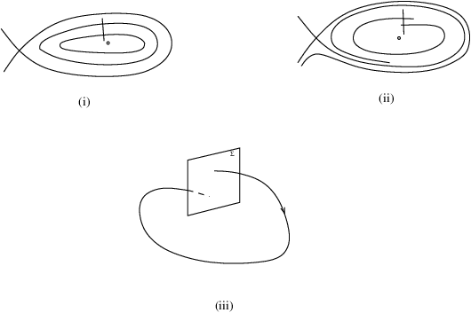
{\cal P}_{l_{0},{\cal F}_{\varepsilon}}:\Sigma\rightarrow\Sigma\;.

Refer to caption — Figure 1: The first return map and its complexification.

In the case when $l_{0}$ is an oval of the real polynomial $f$ , it is just the complexification of the analytic Poincaré map ${\cal P}_{\varepsilon}$ defined above, see Fig. 1. In general, the definition of ${\cal P}_{l_{0},{\cal F}_{\varepsilon}}$ is the following, see e.g. [17]. Let ${\cal F}_{0}^{\perp}$ be a holomorphic foliation transversal to ${\cal F}_{0}=\{df=0\}$ in some neighborhood of $l_{0}$ (for instance, ${\cal F}_{0}^{\perp}=\{f_{y}dx-f_{x}dy=0\}$ ). Then for $|\varepsilon|$ sufficiently small, ${\cal F}_{0}^{\perp}$ remains transversal to ${\cal F}_{\varepsilon}$ . The holonomy map ${\cal P}_{l_{0},{\cal F}_{\varepsilon}}$ is a germ of a biholomorphic map in a neighborhood of $P_{0}\in\Sigma$ which is obtained by lifting the loop $l_{0}$ in the leaves of ${\cal F}_{\varepsilon}$ via ${\cal F}_{0}^{\perp}$ . Namely, $Q={\cal P}_{l_{0},{\cal F}_{\varepsilon}}(P)$ if there exists a path $\tilde{l_{0}}$ in a leaf of ${\cal F}_{\varepsilon}$ which connects $P$ and $Q$ , and which is a lift of the loop $l_{0}$ according to ${\cal F}_{0}^{\perp}$ . The holonomy map ${\cal P}_{l_{0},{\cal F}_{\varepsilon}}$ does not depend on the choice of the transversal foliation ${\cal F}_{0}^{\perp}$ . If $l_{0},l_{1}$ are two homotopic loops with the same initial point $P_{0}$ , then ${\cal P}_{l_{0},{\cal F}_{\varepsilon}}={\cal P}_{l_{1},{\cal F}_{\varepsilon}}$ .

Let us fix the foliation ${\cal F}_{\varepsilon}$ and the loop $l_{0}$ . As before, if we suppose that ${\cal P}_{l_{0},{\cal F}_{\varepsilon}}\neq id$ , then there exists $k\in\mbox{\of N}$ such that

{\cal P}_{l_{0},{\cal F}_{\varepsilon}}(t)=t+\varepsilon^{k}M_{k}(l_{0},{\cal F}_{\varepsilon},t)+...

When there is no danger of confusion, we shall write simply

M_{k}(l_{0},{\cal F}_{\varepsilon},t)=M_{k}(t).

The function $M_{k}$ is called the generating function associated to the unfolding ${\cal F}_{\varepsilon}$ and to the loop $l_{0}$ . Note that the natural number $k$ as well as $M_{k}$ depend on $l_{0},{\cal F}_{\varepsilon}$ and $\Sigma$ in general. The following observation is crucial for the rest of the paper.

Proposition 1

The number $k$ and the generating function $M_{k}$ do not depend on $\Sigma$ . They depend on the foliation ${\cal F}_{\varepsilon}$ and on the free homotopy class of the loop $l_{0}\subset f^{-1}(t)$ . The generating function $M_{k}(t)$ allows an analytic continuation on the universal covering of $\mbox{\of C}\setminus\Delta$ , where $\Delta$ is the set of atypical points of $f$ .

The proof the proposition uses the following algebraic lemma.

Lemma 1

Take $k\in\mbox{\of N}$ . Let

P_{\varepsilon}(t)=t+\sum_{i=k}^{\infty}\varepsilon^{i}p_{i}(t),\quad p_{k}\neq 0,\quad G_{\varepsilon}(t)=t+\sum_{i=1}^{\infty}\varepsilon^{i}g_{i}(t)

be convergent power series of $(t,\varepsilon)$ in a suitable polydisc centered at the origin in $\mbox{\of C}^{2}$ . If $\varepsilon$ is fixed and sufficiently small, then $G_{\varepsilon}$ is a local automorphism and

G_{\varepsilon}^{-1}\circ P_{\varepsilon}\circ G_{\varepsilon}(t)=t+\sum_{i=k}^{\infty}\varepsilon^{i}\tilde{p}_{i}(t)

where $\tilde{p}_{k}(t)\equiv p_{k}(t)$ .

Proof of Lemma 1. We have

	$\displaystyle P_{\varepsilon}\circ G_{\varepsilon}(t)$	$\displaystyle=$	$\displaystyle G_{\varepsilon}(t)+\sum_{i=k}^{\infty}\varepsilon^{i}p_{i}(G_{\varepsilon}(t))=G_{\varepsilon}(t)+\varepsilon^{k}p_{k}(t)+{\rm O}(\varepsilon^{k+1})$
	$\displaystyle G_{\varepsilon}^{-1}(t)$	$\displaystyle=$	$\displaystyle t+\sum_{i=1}^{\infty}\varepsilon^{i}\tilde{g}_{i}(t)$

and therefore

$\displaystyle G_{\varepsilon}^{-1}\circ P_{\varepsilon}\circ G_{\varepsilon}(t)$	$\displaystyle=$	$\displaystyle G_{\varepsilon}(t)+\varepsilon^{k}p_{k}(t)+{\rm O}(\varepsilon^{k+1})$
	$\displaystyle+$	$\displaystyle\sum_{i=1}^{\infty}\varepsilon^{i}\tilde{g}_{i}(G_{\varepsilon}(t)+\varepsilon^{k}p_{k}(t)+{\rm O}(\varepsilon^{k+1}))$
	$\displaystyle=$	$\displaystyle G_{\varepsilon}(t)+\varepsilon^{k}p_{k}(t)+\sum_{i=1}^{\infty}\varepsilon^{i}\tilde{g}_{i}(G_{\varepsilon}(t))+{\rm O}(\varepsilon^{k+1})$
	$\displaystyle=$	$\displaystyle G_{\varepsilon}^{-1}\circ G_{\varepsilon}(t)+\varepsilon^{k}p_{k}(t)+{\rm O}(\varepsilon^{k+1})$
	$\displaystyle=$	$\displaystyle t+\varepsilon^{k}p_{k}(t)+{\rm O}(\varepsilon^{k+1}).$

In the above computation ${\rm O}(\varepsilon^{k+1})$ denotes a power series in $t,\varepsilon$ containing terms of degree at least $k+1$ in $\varepsilon$ . The lemma is proved.

Proof of Proposition 1. Let $\tilde{\Sigma}$ be another transversal disc centered at $P_{0}$ and

\tilde{{\cal P}}_{l_{0},{\cal F}_{\varepsilon}}(t):\tilde{\Sigma}\rightarrow\tilde{\Sigma}

the corresponding holonomy map. Then

{\cal P}_{l_{0},{\cal F}_{\varepsilon}}(t)=G_{\varepsilon}^{-1}\circ\tilde{{\cal P}}_{l_{0},{\cal F}_{\varepsilon}}(t)\circ G_{\varepsilon}(t)

where

G_{\varepsilon}:\Sigma\rightarrow\tilde{\Sigma}

is analytic and $G_{0}(t)\equiv t$ . Lemma 1 shows that

\tilde{{\cal P}}_{l_{0},{\cal F}_{\varepsilon}}(t)=t+\varepsilon^{k}M_{k}(t)+{\rm O}(\varepsilon^{k+1}),\quad M_{k}(t)\not\equiv 0

if and only if

{\cal P}_{l_{0},{\cal F}_{\varepsilon}}(t)=t+\varepsilon^{k}M_{k}(t)+{\rm O}(\varepsilon^{k+1}),\quad M_{k}(t)\not\equiv 0

As the holonomy map ${\cal P}_{l_{0},{\cal F}_{\varepsilon}}(t)$ depends on the homotopy class of $l_{0}$ this holds true for $k$ and $M_{k}$ . In contrast to ${\cal P}_{l_{0},{\cal F}_{\varepsilon}}$ , the generating function $M_{k}$ depends on the free homotopy class of $l_{0}$ . Indeed, let $\tilde{l}_{0}$ be a path in $f^{-1}(t_{0})$ starting at $Q_{0}$ and terminating at $P_{0}$ , and let $\tilde{\Sigma}$ be a transversal disc centered at $Q_{0}$ with corresponding holonomy map

\tilde{{\cal P}}_{l_{0},{\cal F}_{\varepsilon}}(t):\tilde{\Sigma}\rightarrow\tilde{\Sigma}.

Then we have

{\cal P}_{l_{0},{\cal F}_{\varepsilon}}(t)=G_{\tilde{l}_{0},{\cal F}_{\varepsilon}}^{-1}\circ\tilde{{\cal P}}_{l_{0},{\cal F}_{\varepsilon}}(t)\circ G_{\tilde{l}_{0},{\cal F}_{\varepsilon}}(t)

(6)

where

G_{\tilde{l}_{0},{\cal F}_{\varepsilon}}:\Sigma\rightarrow\tilde{\Sigma}

is analytic and $G_{\tilde{l}_{0},{\cal F}_{0}}(t)\equiv t$ (the definition of $G_{\tilde{l}_{0},{\cal F}_{\varepsilon}}$ is similar to the definition of ${\cal P}_{l_{0},{\cal F}_{\varepsilon}}(t)$ ). Lemma 1 shows that the generating function $M_{k}(t)$ does not depend on the special choice of the initial point $P_{0}$ . We conclude that it depends only on the free homotopy class of the loop $l_{0}$ . Until now $M_{k}$ was defined only locally (on the transversal disc $\Sigma$ ). As the fibration $\mbox{\of C}^{2}\setminus f^{-1}(\Delta)\stackrel{{\scriptstyle f}}{{\rightarrow}}\mbox{\of C}\setminus\Delta$ is locally trivial, then each closed loop $l_{0}\in f^{-1}(t_{0})$ defines a continuous family $l_{0}(t)$ of closed loops on $f^{-1}(t)$ , defined on the universal covering space of $\mbox{\of C}\setminus\Delta$ . Only the free homotopy classes of the loops $l_{0}(t)$ are well defined and to each $l_{0}(t)$ corresponds a holonomy map defined up to conjugation, see (6). As this conjugation preserves the number $k$ and the generating function $M_{k}(t)$ then the latter allows an analytic continuation on the universal covering of $\mbox{\of C}\setminus\Delta$ . Proposition 1 is proved. $\Box$

The monodromy group of $M_{k}(t)$ is defined as follows. The function $M_{k}(t)$ is multivalued on $\mbox{\of C}\setminus\Delta$ . Let us consider all its possible determinations in a sufficiently small neighborhood of $t=t_{0}$ . All integer linear combinations of such functions form a module over ℤ which we denote by ${\cal M}_{k}(l_{0},{\cal F}_{\varepsilon})$ . When there is no danger of confusion we shall write simply

{\cal M}_{k}(l_{0},{\cal F}_{\varepsilon})={\cal M}_{k}.

The fundamental group $\pi_{1}(\mbox{\of C}\setminus\Delta,t_{0})$ acts on ${\cal M}_{k}$ as follows. If $\gamma\in\pi_{1}(\mbox{\of C}\setminus\Delta,t_{0})$ and $M\in{\cal M}_{k}$ , let $\gamma_{*}M(t)$ be the analytic continuation of $M(t)$ along $\gamma$ . Then $\gamma_{*}$ is an automorphism of ${\cal M}_{k}$ and

(\gamma_{1}\circ\gamma_{2})_{*}M=\gamma_{2*}(\gamma_{1*}M)\;.

Definition 2

The monodromy representation associated to the generating function $M_{k}$ is the group homomorphism

\pi_{1}(\mbox{\of C}\setminus\Delta,t_{0})\rightarrow Aut({\cal M}_{k})\;.

(7)

The group image of $\pi_{1}(\mbox{\of C}\setminus\Delta,t_{0})$ under $(\ref{repr})$ is called the monodromy group of $M_{k}$ .

In what follows we wish to clarify the case when the generating function is (or is not) an Abelian integral. For this we need to know the monodromy representation of $M_{k}$ .

2.2 The universal monodromy representation of the generating function

Let $H$ be a group and $S\subset H$ a set. We construct an abelian group $\hat{S}/[H,\hat{S}]$ associated to the pair $H,S$ as follows. Let $\hat{S}$ be the group generated by the set

\{hsh^{-1}:h\in H\},

that is to say, the least normal subgroup of $H$ containing $S$ . We denote by $[H,\hat{S}]$ the “commutator” group generated by

\{hsh^{-1}s^{-1}:h\in H,\;s\in\hat{S}\}.

Then $[H,\hat{S}]=[\hat{S},H]$ is a normal subgroup of $\hat{S}$ and $\hat{S}/[H,\hat{S}]$ is an abelian group. There is a canonical homomorphism

\hat{S}/[H,\hat{S}]\rightarrow H/[H,H]

which is not injective in general. Note that $\hat{S}=H$ implies that $\hat{S}/[H,\hat{S}]=H/[H,H]$ is the abelianization of $H$ .

We apply now the above construction to the case when $H=\pi_{1}(\Gamma,P_{0})$ is the fundamental group of a connected surface $\Gamma$ (not necessarily compact), $P_{0}\in\Gamma$ . Let $\pi_{1}(\Gamma)$ be the set of immersions of the circle into $\Gamma$ , up to homotopy equivalence (the set of free homotopy classes of closed loops). Let $S\subset\pi_{1}(\Gamma)$ be a set and $\hat{S}\subset\pi_{1}(\Gamma,P_{0})$ be the pre-image of $S$ under the canonical projection

\pi_{1}(\Gamma,P_{0})\rightarrow\pi_{1}(\Gamma)\;.

Then $\hat{S}$ is a normal subgroup of $\pi_{1}(\Gamma,P_{0})$ and we define

H^{S}_{1}(\Gamma,\mbox{\of Z})=\hat{S}/[\hat{S},\pi_{1}(\Gamma,P_{0})].

In the case when $\hat{S}=\pi_{1}(\Gamma,P_{0})$ we have $H^{S}_{1}(\Gamma,\mbox{\of Z})=H_{1}(\Gamma,\mbox{\of Z})$ , the first homology group of $\Gamma$ . Let $\Psi$ be a diffeomorphism of $\Gamma$ . It induces a map

\Psi_{*}:\pi_{1}(\Gamma)\rightarrow\pi_{1}(\Gamma)

and we suppose that $\Psi_{*}(S)=S$ . Then it induces an automorphism (denoted again by $\Psi*$ )

\Psi_{*}:H^{S}_{1}(\Gamma,\mbox{\of Z})\rightarrow H^{S}_{1}(\Gamma,\mbox{\of Z}).

Note also that if $\Psi_{0}$ is a diffeomorphism isotopic to the identity, then it induces the identity automorphism.

Two closed loops $s_{1},s_{2}\in\hat{S}$ represent the same free homotopy class if and only if $s_{1}=hs_{2}h^{-1}$ for some $h\in\pi_{1}(\Gamma,P_{0})$ . It follows that to each free homotopy class of closed loops represented by an element of $\hat{S}$ there corresponds a unique element of $H^{S}_{1}(\Gamma,\mbox{\of Z})$ .

Consider finally the locally trivial fibration

\mbox{\of C}^{2}\setminus f^{-1}(\Delta)\stackrel{{\scriptstyle f}}{{\rightarrow}}\mbox{\of C}\setminus\Delta

defined by the non-constant polynomial $f\in\mbox{\of C}[x,y]$ and put $\Gamma=f^{-1}(t_{0})$ , $t_{0}\not\in\Delta$ . Each loop $\gamma\in\pi_{1}(\mbox{\of C}\setminus\Delta,t_{0})$ induces a diffeomorphism $\gamma_{*}$ of $\Gamma$ , defined up to an isotopy, and hence a canonical group homomorphism

\pi_{1}(\mbox{\of C}\setminus\Delta,t_{0})\rightarrow\mbox{\rm Diff}\,(\Gamma)/\mbox{\rm Diff}_{0}(\Gamma).

(8)

Here ${\rm Diff}\,(\Gamma)/\mbox{\rm Diff}_{0}(\Gamma)$ denotes the group of diffeomorphisms ${\rm Diff}\,(\Gamma)$ of $\Gamma$ , up to diffeomorphisms ${\rm Diff}_{0}\,(\Gamma)$ isotopic to the identity (the so called mapping class group of $\Gamma$ ). The homomorphism (8) induces a homomorphism (group action on $\pi_{1}(\Gamma)$ )

\pi_{1}(\mbox{\of C}\setminus\Delta,t_{0})\rightarrow\mbox{\it Perm}\,(\pi_{1}(\Gamma))

(9)

where $\mbox{\it Perm}\,(\pi_{1}(\Gamma))$ is the group of permutations of $\pi_{1}(\Gamma)$ .

Let $l_{0}\in\Gamma$ be a closed loop, and let $\hat{S}\subset\pi_{1}(f^{-1}(t_{0}),P_{0})$ be the subgroup “generated” by $l_{0}$ . More precisely, let $\bar{l_{0}}\in\pi_{1}(f^{-1}(t_{0}))$ be the free homotopy equivalence class represented by $l_{0}$ . We denote by $S\subset\pi_{1}(\Gamma)$ the orbit $\pi_{1}(\mbox{\of C}\setminus\Delta,t_{0})\bar{l_{0}}$ . Let $\hat{S}\subset\pi_{1}(\Gamma,P_{0})$ be the subgroup generated by the pre-image of the orbit ${\cal O}_{l_{0}}$ under the canonical map

\pi_{1}(\Gamma,P_{0})\rightarrow\pi_{1}(\Gamma)\;

and let us put

H^{l_{0}}_{1}(\Gamma,\mbox{\of Z})=\hat{S}/[\pi_{1}(\Gamma,P_{0}),\hat{S}].

We obtain therefore the following

Proposition 2

The group $H^{l_{0}}_{1}(f^{-1}(t_{0}),\mbox{\of Z})$ is abelian and the canonical map

H^{l_{0}}_{1}(f^{-1}(t_{0}),\mbox{\of Z})\rightarrow H_{1}(f^{-1}(t_{0}),\mbox{\of Z})

(10)

is a homomorphism. The group action $(\ref{action1})$ of $\pi_{1}(\mbox{\of C}\setminus\Delta,t_{0})$ on $\pi_{1}(f^{-1}(t_{0}))$ induces a homomorphism

\pi_{1}(\mbox{\of C}\setminus\Delta,t_{0})\rightarrow Aut(H^{l_{0}}_{1}(f^{-1}(t_{0}),\mbox{\of Z}))

(11)

called the monodromy representation associated to the loop $l_{0}$ .

The monodromy group associated to $l_{0}$ is the group image of $\pi_{1}(\mbox{\of C}\setminus\Delta,t_{0})$ under the group homomorphism (11).

Theorem 1

For every polynomial deformation ${\cal F}_{\varepsilon}$ of the foliation $df=0$ , and every closed loop $l_{0}\subset f^{-1}(t_{0})$ , the monodromy representation $(\ref{repr})$ of the generating function $M_{k}$ is a sub-representation of the monodromy representation dual to $(\ref{monodromy1})$ .

The concrete meaning of the above theorem is as follows. There exists a canonical surjective homomorphism

H^{l_{0}}_{1}(f^{-1}(t_{0}),\mbox{\of Z})\stackrel{{\scriptstyle\varphi}}{{\rightarrow}}{\cal M}_{k}(l_{0},{\cal F}_{\varepsilon})

(12)

compatible with the action of $\pi_{1}(\mbox{\of C}\setminus\Delta,t_{0})$ . The latter means that for every $\gamma\in\pi_{1}(\mbox{\of C}\setminus\Delta,t_{0})$ the diagram

$\displaystyle H^{l_{0}}_{1}(f^{-1}(t_{0}),\mbox{\of Z})$	$\displaystyle\stackrel{{\scriptstyle\varphi}}{{\rightarrow}}$	$\displaystyle{\cal M}_{k}(l_{0},{\cal F}_{\varepsilon})$
$\displaystyle\downarrow\gamma_{*}$		$\displaystyle\downarrow\gamma_{*}$
$\displaystyle H^{l_{0}}_{1}(f^{-1}(t_{0}),\mbox{\of Z})$	$\displaystyle\stackrel{{\scriptstyle\varphi}}{{\rightarrow}}$	$\displaystyle{\cal M}_{k}(l_{0},{\cal F}_{\varepsilon})$

commutes ( $\gamma_{*}$ is the automorphism induced by $\gamma$ ). Therefore $Ker(\varphi)$ is a subgroup of $H^{l_{0}}_{1}(f^{-1}(t_{0}),\mbox{\of Z})$ , invariant under the action $\pi_{1}(\mbox{\of C}\setminus\Delta,t_{0})$ , and hence (7) is isomorphic to the induced representation

\pi_{1}(\mbox{\of C}\setminus\Delta,t_{0})\rightarrow H^{l_{0}}_{1}(f^{-1}(t_{0}),\mbox{\of Z})/Ker(\varphi)

which is a subrepresentation of

\pi_{1}(\mbox{\of C}\setminus\Delta,t_{0})\rightarrow H^{l_{0}}_{1}(f^{-1}(t_{0}),\mbox{\of Z})^{*}.

Proof of Theorem 1. First of all, note that if $l_{1},l_{2}\in\pi_{1}(f^{-1}(t_{0}),P_{0})$ and

{\cal P}_{l_{1},{\cal F}_{\varepsilon}}(t)=t+M_{k}(l_{1},{\cal F}_{\varepsilon},t)\varepsilon^{k}+{\rm O}(\varepsilon^{k+1}),\;\;{\cal P}_{l_{2},{\cal F}_{\varepsilon}}(t)=t+M_{k}(l_{2},{\cal F}_{\varepsilon},t)\varepsilon^{k}+{\rm O}(\varepsilon^{k+1})

then

{\cal P}_{l_{1},{\cal F}_{\varepsilon}}\circ{\cal P}_{l_{2},{\cal F}_{\varepsilon}}(t)={\cal P}_{l_{2}\circ l_{1},{\cal F}_{\varepsilon}}(t)=t+(M_{k}(l_{1},{\cal F}_{\varepsilon},t)+M_{k}(l_{2},{\cal F}_{\varepsilon},t))\varepsilon^{k}+{\rm O}(\varepsilon^{k+1})

(the proof repeats the arguments of Proposition 1). It follows that

M_{k}(l_{1}\circ l_{2},{\cal F}_{\varepsilon},t)=M_{k}(l_{2}\circ l_{1},{\cal F}_{\varepsilon},t)=M_{k}(l_{1},{\cal F}_{\varepsilon},t)+M_{k}(l_{2},{\cal F}_{\varepsilon},t).

(13)

The generating function $M_{k}(t)$ is locally analytic and multivalued on $\mbox{\of C}\setminus\Delta$ . For every determination $\gamma_{*}M_{k}(l_{0},{\cal F}_{\varepsilon},t)$ of $M_{k}(l_{0},{\cal F}_{\varepsilon},t)$ obtained after an analytic continuation along a closed loop $\gamma\in\pi_{1}(\mbox{\of C}\setminus\Delta,t_{0})$ it holds

\gamma_{*}M_{k}(l_{0},{\cal F}_{\varepsilon},t))=M_{k}(\gamma_{*}l_{0},{\cal F}_{\varepsilon},t)

(14)

where $l_{0}$ is (by abuse of notation) a free homotopy class of closed loops on $f^{-1}(t_{0})$ . Indeed, let $l(t)\subset f^{-1}(t)$ be a continuous family of closed loops, $l(t_{0})=l_{0}$ . For each $\tilde{t}_{0}$ we may define a holonomy map ${\cal P}_{l(\tilde{t}_{0}),{\cal F}_{\varepsilon}}(t)$ analytic in a sufficiently small disc centered at $\tilde{t}_{0}$ . It follows from the definition of the holonomy map, that if $\tilde{t}_{0},t_{0}$ are fixed sufficiently close regular values of $f$ , then ${\cal P}_{l(\tilde{t_{0}}),{\cal F}_{\varepsilon}}(t)$ and ${\cal P}_{l(t_{0}),{\cal F}_{\varepsilon}}(t)$ coincide in some open disc, containing $\tilde{t}_{0},t_{0}$ . The same holds for the corresponding generating functions. This shows that the analytic continuation of $M_{k}(t)=M_{k}(l(t_{0}),{\cal F}_{\varepsilon},t)$ along an interval connecting $t_{0}$ and $\tilde{t}_{0}$ is obtained by taking a continuous deformation of the closed loop $l(t_{0})$ along this interval. Clearly this property of the generating function holds true even without the assumption that $\tilde{t}_{0},t_{0}$ are close and for every path connecting $\tilde{t}_{0},t_{0}$ . This proves the identity (14).

Formula (14) shows that

k(l_{0},{\cal F}_{\varepsilon})=k(\gamma_{*}l_{0},{\cal F}_{\varepsilon}),\quad\forall\gamma\in\pi_{1}(\mbox{\of C}\setminus\Delta,t_{0}).

Let $l\subset f^{-1}(t_{0})$ be a closed loop representing an equivalence class in $H^{l_{0}}_{1}(f^{-1}(t_{0}),\mbox{\of Z})$ . Then (13) implies that $k(l,{\cal F}_{\varepsilon})\geq k(l_{0},{\cal F}_{\varepsilon})$ and we define

\varphi(l)=\left\{\begin{array}[]{ccc}M_{k}(l,{\cal F}_{\varepsilon},t),&&\mbox{ \rm if }k(l,{\cal F}_{\varepsilon})=k(l_{0},{\cal F}_{\varepsilon})\\ 0,&&\mbox{ \rm if }k(l,{\cal F}_{\varepsilon})>k(l_{0},{\cal F}_{\varepsilon})\\ \end{array}\right.

Using the definitions of the abelian groups $H^{l_{0}}_{1}(f^{-1}(t_{0}),\mbox{\of Z})$ and ${\cal M}_{k}(l_{0},{\cal F}_{\varepsilon})$ and the identities (13), (14), it is straightforward to check that

•

$\varphi$ depends on the equivalence class of the loop $l$ in $H^{l_{0}}_{1}(f^{-1}(t_{0}),\mbox{\of Z})$ ;
•

$\varphi(l)$ belongs to ${\cal M}_{k}(l_{0},{\cal F}_{\varepsilon})$ ;
•

$\varphi$ defines a surjective homomorphism (12) which is compatible with the action of $\pi_{1}(\mbox{\of C}\setminus\Delta,t_{0})$ on $H^{l_{0}}_{1}(f^{-1}(t_{0}),\mbox{\of Z})$ and ${\cal M}_{k}(l_{0},{\cal F}_{\varepsilon})$ .

Theorem 1 is proved. $\square$

2.3 Main result

Our main result in this paper is the following.

Theorem 2

1.

If $H^{l_{0}}_{1}(f^{-1}(t_{0}),\mbox{\of Z})$ is of finite dimension, then the generating function $M_{k}(t)=M_{k}(l_{0},{\cal F}_{\varepsilon},t)$ satisfies a linear differential equation

$a_{n}(t)x^{(n)}+a_{n-1}(t)x^{(n-1)}+...+a_{1}(t)x^{\prime}+a_{0}(t)x=0$ (15)

where $n\leq dim\,H^{l_{0}}_{1}(f^{-1}(t_{0}),\mbox{\of Z})$ and $a_{i}(t)$ are suitable analytic functions on $\mbox{\of C}\setminus\Delta$ .
2.

If, moreover, $M_{k}(t)$ is a function of moderate growth at any $t_{i}\in\Delta$ and at $t=\infty$ , then $(\ref{fuchs})$ is an equation of Fuchs type.
3.

If in addition to the preceding hypotheses, the canonical map

$H^{l_{0}}_{1}(f^{-1}(t_{0}),\mbox{\of Z})\rightarrow H_{1}(f^{-1}(t_{0}),\mbox{\of Z})$ (16)

is injective, then $M_{k}(t)$ is an Abelian integral

$M_{k}(t)=\int_{l(t)}\omega$ (17)

where $\omega$ is a rational one-form on $\mbox{\of C}^{2}$ and $l(t)\subset f^{-1}(t)$ is a continuous family of closed loops, $l(t_{0})=l_{0}$ .

Remarks.

1.

Recall that a multivalued locally analytic function $g:\mbox{\of C}\setminus\Delta\rightarrow\mbox{\of C}$ is said to be of moderate growth if for every $\varphi_{0}>0$ there exist constants $C,N>0$ such that

$sup\{|g(t)t^{N}|:0<|t-t_{i}|<C,\;\;\mbox{\it Arg}\,(t-t_{i})<\varphi_{0},\;\;t_{i}\in\Delta\}<\infty$

and

$sup\{|g(t)t^{-N}|:|t|>1/C,\mbox{\it Arg}\,|t|<\varphi_{0}\}<\infty.$
2.

When (16) is not injective, the generating function could still be an Abelian integral. Of course, this depends on the unfolding ${\cal F}_{\varepsilon}$ .
3.

If the dimension of $H^{l_{0}}_{1}(f^{-1}(t_{0}),\mbox{\of Z})$ is finite, we may also suppose that (15) is irreducible. This makes (15) unique (up to a multiplication by analytic functions). The monodromy group of this equation is a subgroup of the monodromy group associated to $l_{0}$ , see (11). It is clear that $M_{k}(t)$ may satisfy other equations with non-analytic coefficients on $\mbox{\of C}\setminus\Delta$ .

Proof of Theorem 2. Suppose that $H^{l_{0}}_{1}(f^{-1}(t_{0}),\mbox{\of Z})$ is of finite dimension. Then ${\cal M}_{k}(l_{0},{\cal F}_{\varepsilon})=H^{l_{0}}_{1}(f^{-1}(t_{0}),\mbox{\of Z})/Ker(\varphi)$ is of finite dimension too, and let $g_{i}(t)=M_{k}(l_{i},{\cal F}_{\varepsilon},t)$ , $i=1,...,n$ be a basis of the complex vector space $V$ generated by ${\cal M}_{k}(l_{0},{\cal F}_{\varepsilon})$ , $\dim_{\mbox{\of C}}V\leq\dim_{\mbox{\of Z}}{\cal M}_{k}(l_{0},{\cal F}_{\varepsilon})$ . There is a unique linear differential equation of order $\dim_{\mbox{\of C}}V$ satisfied by the above generating functions (and hence by $M_{k}(l_{0},{\cal F}_{\varepsilon},t)$ ) having the form (15) which can be equivalently written as

\det\pmatrix{g_{1}&g_{1}^{\prime}&...&g_{1}^{(n)}\cr g_{2}&g_{2}^{\prime}&...&g_{2}^{(n)}\cr.&.&...&.\cr g_{n}&g_{n}^{\prime}&...&g_{n}^{(n)}\cr\cr x&x^{\prime}&...&x^{(n)}}=0.

(18)

The functions $g_{1},g_{2},...,g_{n}$ are linearly independent over ℂ and define a complex vector space invariant under the action of $\pi_{1}(\mbox{\of C}\setminus\Delta,t_{0})$ . For a given $\gamma\in\pi_{1}(\mbox{\of C}\setminus\Delta,t_{0})$ , let $\gamma_{*}\in Aut(V)$ be the automorphism (11) and denote (by abuse of notation) by $\gamma_{*}a_{i}(t)$ the analytic continuation of $a_{i}(t)$ along the loop $\gamma$ . The explicit form of the coefficients $a_{i}(t)$ as determinants (see (18)) implies that $\gamma_{*}a_{i}(t)=det(\gamma_{*})a_{i}(t)$ . Therefore $\gamma_{*}[a_{i}(t)/a_{n}(t)]=a_{i}(t)/a_{n}(t)$ , $a_{i}(t)/a_{n}(t)$ are single-valued and hence meromorphic functions on $\mbox{\of C}\setminus\Delta$ . This proves the first claim of the theorem. If in addition $M_{k}(t)$ is of moderate growth, then $g_{i}(t)$ are of moderate growth too, $a_{i}(t)/a_{n}(t)$ are rational functions, and the equation (15) is of Fuchs type (eventually with apparent singularities).

Suppose finally that (16) is injective, which implies that $H^{l_{0}}_{1}(f^{-1}(t_{0}),\mbox{\of Z})$ is a subgroup of the homology group $H_{1}(f^{-1}(t_{0}),\mbox{\of Z})$ . By the algebraic de Rham theorem [8] the first cohomology group of $f^{-1}(t_{0})$ is generated by polynomial one-forms. In particular, the dual space of $H^{l_{0}}_{1}(f^{-1}(t_{0}),\mbox{\of Z})$ is generated by polynomial one-forms $\omega_{1},\omega_{2},...,\omega_{n}$ . Let $l_{1}(t),l_{2}(t),...,l_{n}(t),l(t)\subset f^{-1}(t)$ be a continuous family of closed loops, such that $l_{1}(t_{0}),l_{2}(t_{0}),...,l_{n}(t_{0})$ defines a basis of $H^{l_{0}}_{1}(f^{-1}(t_{0}),\mbox{\of Z}$ , $l(t_{0})=l_{0}$ . The determinant

\det\pmatrix{g_{1}&\int_{l_{1}}\omega_{1}&\int_{l_{1}}\omega_{2}&...&\int_{l_{1}}\omega_{n}\cr g_{2}&\int_{l_{2}}\omega_{1}&\int_{l_{2}}\omega_{2}&...&\int_{l_{2}}\omega_{n}\cr.&.&...&.\cr g_{n}&\int_{l_{n}}\omega_{1}&\int_{l_{n}}\omega_{2}&...&\int_{l_{n}}\omega_{n}\cr M_{k}&\int_{l}\omega_{1}&\int_{l}\omega_{2}&...&\int_{l}\omega_{n}}=0.

(19)

developed with respect to the last row gives

\alpha_{0}M_{k}+\alpha_{1}\int_{l}\omega_{1}+\alpha_{2}\int_{l}\omega_{2}+...\alpha_{n}\int_{l}\omega_{n}=0.

As $H^{l_{0}}_{1}(f^{-1}(t_{0}),\mbox{\of Z})\subset H_{1}(f^{-1}(t_{0}),\mbox{\of Z})$ is invariant under the action of $\pi_{1}(\mbox{\of C}\setminus\Delta,t_{0})$ , then we deduce in the same way as before that $\alpha_{i}(t)/\alpha_{0}(t)$ are rational functions. This completes the proof of the theorem. $\square$

We conclude the present section with some open questions. Let $l_{0}(t)\subset f^{-1}(t)$ be a continuous family of ovals defined by the real polynomial $f\in\mbox{\of R}[x,y]$ .

Open questions

1.

Is it true that the abelian group $H^{l_{0}}_{1}(f^{-1}(t_{0}),\mbox{\of Z})$ is free, torsion free, finitely generated, or even stronger, $\dim H^{l_{0}}_{1}(f^{-1}(t_{0}),\mbox{\of Z})\leq dimH_{1}(f^{-1}(t_{0}),\mbox{\of Z})$ ? If not, give counter-examples.
2.

Is it true that every generating function of a polynomial deformation ${\cal F}_{\varepsilon}$ of $df=0$ is of moderate growth at any point $t\in\Delta$ or $t\in\infty$ ?
3.

Is it true that the monodromy representation (11) has the following universal property : for every $l\in H^{l_{0}}_{1}(f^{-1}(t_{0}),\mbox{\of Z})$ there exists a polynomial deformation ${\cal F}_{\varepsilon}$ of $df=0$ , such that the corresponding generating function $\varphi(l)$ is not identically zero. If this were true it would imply that $H^{l_{0}}_{1}(f^{-1}(t_{0}),\mbox{\of Z})$ is torsion-free, and whenever (16) is not injective, then there exists a polynomial unfolding with corresponding generating function which is not an Abelian integral of the form (17).
4.

Suppose that the canonical homomorphism (10) is surjective. Is it true that it is also injective? Note that a negative answer would imply that the representation (11) is not universal (in the sense of the preceding question). Indeed, if (10) is surjective, then the orbit ${\cal O}_{l_{0}}$ generates the homology group, and hence the generating function is always an Abelian integral. The kernel of the canonical map (10) consist of free homotopy classes (modulo an equivalence relation) homologous to zero, along which every Abelian integral vanishes.

3 Examples

In this section we show that the claims of Theorem 2 are non-empty. Namely, we apply it to polynomial deformations $f$ of the simple singularities $y^{2}+x^{4}$ , $xy(x-y)$ of type $A_{3}$ , $D_{4}$ respectively (see [1, vol. 1] for this terminology). For a given loop $\delta(t)\subset f^{-1}(t)\subset\mbox{\of C}^{2}$ we shall compute the group $H_{1}^{\delta}(f^{-1}(t),\mbox{\of Z})$ . As the abelian groups $H_{1}^{\delta}(f^{-1}(t),\mbox{\of Z})$ are isomorphic, then when the choice of $t$ is irrelevant we shall omit it. The same convention will be applied to the cycles or closed loops on the fibers $f^{-1}(t)$ . An equivalence class of loops in $H_{1}^{\delta}(f^{-1}(t_{0})_{t},\mbox{\of Z})$ will be represented by a free homotopy class of loops on $f^{-1}(t)$ . Two such free homotopy classes $\delta_{1},\delta_{2}$ are composed in the following way: take any two representative of $\delta_{1},\delta_{2}$ in the fundamental group of the surface $f^{-1}(t)$ and compose them. This operation is compatible with the group law in $H_{1}^{\delta}(f^{-1}(t_{0})_{t},\mbox{\of Z})$ , provided that $\delta_{1},\delta_{2}$ represent equivalence classes in it. The operation defines a unique element in $H_{1}^{\delta}(f^{-1}(t_{0})_{t},\mbox{\of Z})$ (represented once again by a non-unique free homotopy class of loops).

3.1 The $A_{3}$ singularity

Take

f(x,y)=\frac{y^{2}}{2}+\frac{(x^{2}-1)^{2}}{4}

and denote by $\delta_{e}(t),\delta_{l}(t),\delta_{r}(t)$ respectively the exterior, left interior and right interior continuous family of ovals defined by $\{(x,y)\in\mbox{\of R}^{2}:f(x,y)=t\}$ , see Fig. 2.

We denote by the same letters the corresponding continuous families of free homotopy classes of loops defined on the universal covering space of $\mbox{\of C}\setminus\{0,1/4\}$ , and fix $t_{0}\neq 0$ .

Proposition 3

We have

H^{\delta_{l}}_{1}(f^{-1}(t_{0}),\mbox{\of Z})=H^{\delta_{r}}_{1}(f^{-1}(t_{0}),\mbox{\of Z})=H_{1}(f^{-1}(t_{0}),\mbox{\of Z})=\mbox{\of Z}^{3},\quad H_{\delta_{e}(t_{0})}=\mbox{\of Z}^{2}

and the canonical map $H^{\delta_{e}}_{1}(f^{-1}(t_{0}),\mbox{\of Z})\rightarrow H_{1}(f^{-1}(t_{0}),\mbox{\of Z})$ is injective.

Applying Theorem 2 we get

Corollary 1

For every polynomial unfolding ${\cal F}_{\varepsilon}$ the generating function $M_{\delta_{e}(t_{0})}$ is an Abelian integral, provided that this function is of moderate growth.

It is possible to show that $M_{\delta_{e}(t_{0})}$ is always of moderate growth (this will follow from the explicit computations below). As for $M_{\delta_{l}(t_{0})}$ and $M_{\delta_{r}(t_{0})}$ , it follows from [5] that these functions are always Abelian integrals.

Proof of Proposition 3. The affine curve $f^{-1}(t_{0})$ is a torus with two removed points, and hence $H_{1}(f^{-1}(t_{0}),\mbox{\of Z})=\mbox{\of Z}^{3}$ . We compute first $H^{\delta_{l}}_{1}(f^{-1}(t_{0}),\mbox{\of Z})$ . Let $t_{0}\in(0,1/4)$ and let $\delta_{s}(t)\subset f^{-1}(t)$ , $t\in(0,1/4)$ , be the continuous family of “imaginary” closed loops (the ovals of $\{y^{2}/2-(x^{2}-1)^{2}/4=t\}$ ) which tend to the saddle point $(0,0)$ as $t$ tends to $1/4$ . As before we denote by the same letter the continuous family of free homotopy classes of loops defined on the universal covering space of $\mbox{\of C}\setminus\{0,1/4\}$ , and fix $t_{0}\neq 0,1/4$ . Let $l_{0},l_{1/4}\in\pi_{1}(\mbox{\of C}\setminus\{0,1/4\},t_{0})$ be two simple loops making one turn about $0$ and $1/4$ respectively in a positive direction. The group $\pi_{1}(\mbox{\of C}\setminus\{0,1/4\},t_{0})$ acts on $\pi_{1}(f^{-1}(t_{0}))$ as follows. To the loop $l_{1/4}$ corresponds an automorphism of $f^{-1}(t_{0})$ which is a Dehn twist along $\delta_{s}(t_{0})$ . Recall that a Dehn twist of a surface along a closed loop is a diffeomorphism which is the identity, except in a neighborhood of the loop. In a neighborhood of the loop the diffeomorphism is shown on Fig. 3, see [22]. The usual Picard-Lefschetz formula [1] describes an automorphism of the homology group induced by a Dehn twist along a “vanishing” loop.

Therefore $l_{1/4*}\delta_{s}=\delta_{s}$ and $l_{1/4*}\delta_{l}$ is the loop shown on Fig. 3. We may also compose the loops $\delta_{s},l_{1/4*}\delta_{l}$ in the way explained in the beginning of this section. The result is an equivalence class in $H^{\delta_{l}}_{1}(f^{-1}(t_{0}),\mbox{\of Z})$ represented in a non-unique way by a closed loop. The equivalence class $\mbox{\it Var}_{l_{1/4}}\delta_{l}=(l_{1/4}-id)_{*}\delta_{l}$ equals therefore to the class represented by $\delta_{s}$ , and hence $\mbox{\it Var}_{l_{1/4}}^{2}\delta_{l}$ represents the zero class. In a similar way we compute $l_{0*}\delta_{s}(t_{0})$ which equals $\delta_{s}+\delta_{r}+\delta_{l}$ , as well as its first variation $\mbox{\it Var}_{l_{0}}\delta_{s}=(l_{0}-id)_{*}\delta_{s}$ which equals $\delta_{r}+\delta_{l}$ , see Fig. 5. It follows that the second variation $\mbox{\it Var}^{2}_{l_{0}}\delta_{s}$ of $\delta_{s}$ may be represented by a loop homotopic to a point. We conclude that $H^{\delta_{l}}_{1}(f^{-1}(t_{0}),\mbox{\of Z})$ is generated by equivalence classes represented by $\delta_{l},\delta_{s},\delta_{r}$ and hence it coincides with $H_{1}(f^{-1}(t_{0}),\mbox{\of Z})$ (generated by the same loops). The computation of $H^{\delta_{r}}_{1}(f^{-1}(t_{0}),\mbox{\of Z})$ is analogous.

To compute $H^{\delta_{e}}_{1}(f^{-1}(t_{0}),\mbox{\of Z})$ we note that this group coincides with $H^{\delta_{s}}_{1}(f^{-1}(t_{0}),\mbox{\of Z})$ . Indeed, take a loop $l\subset\mbox{\of C}$ starting at $t_{0}\in(0,1/4)$ and terminating at some $t_{1}\in(1/4,\infty)$ as it is shown on Fig. 4. This defines a continuous family of (free homotopy classes of) loops $\delta_{s}(t)$ along $l$ . Then it follows from Fig. 4 that

\delta_{s}(t_{0})=\delta_{e}(t_{1})\;

and hence $H^{\delta_{s}(t_{0})}_{1}(f^{-1}(t_{0}),\mbox{\of Z})=H^{\delta_{e}(t_{1})}_{1}(f^{-1}(t_{0}),\mbox{\of Z})$ . The loop $l_{0*}\delta_{s}(t_{0})$ and its first variation $\mbox{\it Var}_{l_{0}}\delta_{s}(t_{0})=(l_{0}-id)_{*}\delta_{s}(t_{0})$ were already computed (Fig. 5)

and the second variation $\mbox{\it Var}^{2}_{l_{0}}\delta_{s}(t_{0})$ may be represented by a loop homotopic to a point. Further, $l_{1/4*}\delta_{s}(t_{0})=\delta_{s}(t_{0})$ , and the first variation $\mbox{\it Var}_{l_{1/4}}\mbox{\it Var}_{l_{0}}\delta_{s}(t_{0})$ of $\mbox{\it Var}_{l_{0}}\delta_{s}(t_{0})$ along $l_{1/4}$ is a composition of free homotopy classes of $\delta_{s}$ (two times). It follows that $H^{\delta_{s}}_{1}(f^{-1}(t_{0}),\mbox{\of Z})$ is generated by $\delta_{s}$ and $\mbox{\it Var}_{l_{0}}\delta_{s}$ . As these loops are homologically independent we conclude that

H^{\delta_{s}}_{1}(f^{-1}(t_{0}),\mbox{\of Z})\rightarrow H_{1}(f^{-1}(t_{0}),\mbox{\of Z})

is injective and $H^{\delta_{s}}_{1}(f^{-1}(t_{0}),\mbox{\of Z})=\mbox{\of Z}^{2}$ . The proposition is proved. $\square$

3.2 Calculation of the generating function in the $A_{3}$ case

In what follows we compare the above geometric approach to the combinatorial approach based on Françoise’s recursion formulae. We shall prove a stronger result allowing us to set up an explicit upper bound to the number of zeros in $\Sigma$ of the displacement map ${\cal P}_{\varepsilon}(t)-t$ for small $\varepsilon$ . Below we use the standard notation $H$ of the Hamiltonian function,

H=\frac{y^{2}}{2}+\frac{(x^{2}-1)^{2}}{4}.

We say that $A$ is a polynomial of weighted degree $m$ in $x,y,H$ provided that

A(x,y,H)=\sum_{i+j+2k\leq m}a_{ijk}x^{i}y^{j}H^{k}

(namely, the weight of $x,y$ is one and the weight of $H$ is assumed to be two). Clearly, a polynomial in $x,y$ allows a representation through different weighted polynomials in $x,y,H,$ possibly of different weighted degrees, depending on the way the powers $x^{i}$ with $i>3$ were expressed. However, any polynomial has a unique representation through a weighted polynomial in a normal form which means that the latter contains powers $x^{i}$ with $i\leq 3$ only. We will not assume that the weighted polynomials we consider bellow are taken in a normal form.

Set $\sigma_{k}=x^{k}ydx$ and $I_{k}(t)=\int_{\delta(t)}\sigma_{k}$ , $k=0,1,2,$ where $\delta(t)$ is an oval contained in the level set $\{H=t\}$ .

Proposition 4

For any one-form $\omega_{m}=A_{m}(x,y,H)dx+B_{m}(x,y,H)dy$ with polynomial coefficients of weighted degree $m$ , the following decomposition holds:

\omega_{m}=dG_{m+1}(x,y,H)+g_{m-1}(x,y,H)dH+\alpha_{m-1}(H)\sigma_{0}+\beta_{m-2}(H)\sigma_{1}+\gamma_{m-3}(H)\sigma_{2}

(20)

where $G_{k},g_{k},\alpha_{k},\beta_{k},\gamma_{k}$ are polynomials in their arguments of weighted degree $k$ .

Below, we will denote by $\alpha_{k},\beta_{k},\gamma_{k}$ polynomials of weighted degree $k$ in $H$ , by $G_{k},g_{k}$ polynomials of weighted degree $k$ in $x,y,H$ , and by $\omega_{k}$ one-forms with polynomial coefficients of weighted degree $k$ in $x,y,H$ . (Possibly, different polynomials and one-forms of the same degree and type will be denoted by the same letter.)

Proof of Proposition 4. The proof is similar to the proof of Lemma 1 in [13] which concerned the elliptic case $H=\frac{1}{2}y^{2}+\frac{1}{2}x^{2}-\frac{1}{3}x^{3}$ . It is sufficient to consider the case when the coefficients of the one-form do not depend on $H$ . As in [13], one can easily see that the problem reduces to expressing the one-forms $y^{j}dx,xy^{j}dx,x^{2}y^{j}dx$ in the form (20). We have

\begin{array}[]{rl}y^{j}dx&{\displaystyle\!\!\!=\frac{4j}{2j+1}Hy^{j-2}dx+\frac{j}{2j+1}(x^{2}-1)y^{j-2}dx-\frac{j}{2j+1}xy^{j-2}dH+d\frac{xy^{j}}{2j+1},}\\[8.53581pt] xy^{j}dx&{\displaystyle\!\!\!=\frac{2j}{j+1}Hxy^{j-2}dx-\frac{j}{2j+2}(x^{2}-1)y^{j-2}dH+d\frac{(x^{2}-1)y^{j}}{2j+2},}\\[8.53581pt] x^{2}y^{j}dx&{\displaystyle\!\!\!-\,\frac{1}{2j+3}y^{j}dx=\frac{4j}{2j+3}Hx^{2}y^{j-2}dx-\frac{j}{2j+3}(x^{3}-x)y^{j-2}dH+d\frac{(x^{3}-x)y^{j}}{2j+3}.}\end{array}

¿From the second equation we obtain immediately that $xy^{j}dx=c_{j}H^{\frac{j-1}{2}}\sigma_{1}+dG_{j+2}+g_{j}dH$ ( $c_{j}=0$ for $j$ even, $c_{j}>0$ for $j$ odd) which yields

xA_{m-1}(y)dx=\beta_{m-2}(H)\sigma_{1}+dG_{m+1}+g_{m-1}dH.

Taking notation $\theta_{j}=(y^{j}dx,x^{2}y^{j}dx)^{\top}$ , $\Theta_{j}=(dG_{j+1}+g_{j-1}dH,dG_{j+3}+g_{j+1}dH)^{\top}$ , one can rewrite the system formed by the first and the third equation above in the form

\theta_{j}=\Lambda_{j}(H)\theta_{j-2}+\Theta_{j},\quad\Lambda_{j}(H)=\frac{j}{2j+1}\left(\begin{array}[]{cc}4H-1&1\\[5.69054pt] {\displaystyle\frac{4H-1}{2j+3}}&{\displaystyle\frac{4(2j+1)H+1}{2j+3}}\end{array}\right).

As $\Lambda_{j}\Theta_{j-2}=\Theta_{j}$ , this implies that $\theta_{j}=\Lambda_{j}\Lambda_{j-2}\ldots\Lambda_{3}\theta_{1}+\Theta_{j}$ for $j$ odd and $\theta_{j}=\Lambda_{j}\Lambda_{j-2}\ldots\Lambda_{2}\theta_{0}+\Theta_{j}$ for $j$ even, which in both cases is equivalent to

\begin{array}[]{l}y^{j}dx=\alpha_{j-1}(H)\sigma_{0}+\gamma_{j-3}(H)\sigma_{2}+dG_{j+1}+g_{j-1}dH,\\[5.69054pt] x^{2}y^{j}dx=\alpha_{j-1}(H)\sigma_{0}+\gamma_{j-1}(H)\sigma_{2}+dG_{j+3}+g_{j+1}dH\end{array}

(21)

where the coefficients at $\sigma_{0},\sigma_{2}$ vanish for $j$ even. Applying the last two relations with $j\leq m$ and $j\leq m-2$ respectively, we obtain the result. $\Box$

The above decomposition (20) is the basic tool for calculating the generating functions. For the two period annuli inside the eight-loop (level sets $t\in(0,\frac{1}{4})$ ), one has

\int_{\delta(t)}\omega_{m}=\alpha_{m-1}(t)I_{0}(t)+\beta_{m-2}(t)I_{1}(t)+\gamma_{m-3}(t)I_{2}(t),

and for $0<t<\frac{1}{4}$ ,

\int_{\delta(t)}\omega_{m}\equiv 0\;\;\Leftrightarrow\;\;\alpha_{m-1}(t)=\beta_{m-2}(t)=\gamma_{m-3}(t)\equiv 0\;\;\Leftrightarrow\;\;\omega_{m}=dG_{m+1}+g_{m-1}dH.

This means that the internal period annuli satisfy the so called $(*)$ property [2] and the generating functions are determined from the integration of polynomial one-forms calculated in a recursive procedure. More explicitly, consider a small polynomial perturbation

\begin{array}[]{l}\dot{x}=H_{y}+\varepsilon f(x,y),\\ \dot{y}=-H_{x}+\varepsilon g(x,y),\end{array}

(22)

which can be rewritten as $dH-\varepsilon\omega_{n}=0$ with $\omega_{n}=g(x,y)dx-f(x,y)dy$ and $n$ the degree of the perturbation. Then in $(0,\frac{1}{4})$ , the first nonzero generating function is given by

M_{k}(t)=\int_{\delta(t)}\Omega_{k},\;\;\mbox{\rm where}\;\;\Omega_{1}=\omega_{n},\;\;\Omega_{k}=q_{k-1}\Omega_{1}\;\;\mbox{\rm and}\;\;\Omega_{k-1}=dQ_{k-1}+q_{k-1}dH.

Making use of (20), it is then easily seen by induction that $q_{k-1}$ is a polynomial of weighted degree $(k-1)(n-1)$ , therefore $\Omega_{k}$ is a polynomial one-form of weighted degree $m=k(n-1)+1$ which proves that

M_{k}(t)=\alpha_{[\frac{k(n-1)}{2}]}(t)I_{0}(t)+\beta_{[\frac{k(n-1)-1}{2}]}(t)I_{1}(t)+\gamma_{[\frac{k(n-1)-2}{2}]}(t)I_{2}(t)

(23)

where $\alpha_{j},\beta_{j},\gamma_{j}$ are polynomials in $t$ of degree at most $j$ .

For the period annulus outside the eight-loop (level sets $t\in(\frac{1}{4},\infty)$ ), one has

\int_{\delta(t)}\omega_{m}=\alpha_{m-1}(t)I_{0}(t)+\gamma_{m-3}(t)I_{2}(t),

and for $\frac{1}{4}<t<\infty$ ,

\int_{\delta(t)}\omega_{m}\equiv 0\;\;\Leftrightarrow\;\;\alpha_{m-1}(t)=\gamma_{m-3}(t)\equiv 0\;\;\Leftrightarrow\;\;\omega_{m}=dG_{m+1}+g_{m-1}dH+\beta_{m-2}(H)\sigma_{1}

since $I_{1}(t)\equiv 0$ which is caused by symmetry of the oval. Therefore the outer period annulus does not satisfy the $(*)$ property which makes this case troublesome and we shall deal with it until the end of this section.

Take a point $(x,y)$ lying on a certain level set $H=t$ for a fixed $t>\frac{1}{4}$ and let $(a,0)$ be the intersection point of the level curve with the negative $x$ -axis. Denote by $\delta(x,y)\subset\{H=t\}$ the oriented curve in the $(\xi,\eta)$ plane connecting $(a,0)$ and $(x,y)$ in a clockwise direction. Consider the function $\varphi$ determined by the formula (see formula (2.5) in [11])

\varphi(x,y)=\int_{\delta(x,y)}\frac{\xi d\xi}{\eta}.

As $I_{1}(t)=\int_{\delta(t)}xydx\equiv 0$ , this is also true for $I_{1}^{\prime}(t)=\int_{\delta(t)}\frac{xdx}{y}$ which implies that $\varphi(\pm a,0)=0$ . Therefore, $\varphi(x,y)$ is single-valued and hence an analytic function in the domain outside the eight-loop. In [12], $\varphi$ was expressed as

\varphi(x,y)=\frac{1}{\sqrt{2}}\left({\rm arctan}\frac{x^{2}-1}{y\sqrt{2}}-\frac{\pi}{2}{\rm sign}\,y\right)=\frac{{\rm sign}\,y}{\sqrt{2}}\left({\rm arcsin}\frac{x^{2}-1}{2\sqrt{H}}-\frac{\pi}{2}\right).

In [16], the authors expressed $\varphi$ by a complex logarithmic function

\varphi=\frac{i}{2\sqrt{2}}\log\frac{x^{2}-1+i\sqrt{2}y}{x^{2}-1-i\sqrt{2}y}

and used in their proofs the properties of $\varphi$ on the corresponding Riemann surface. The concrete expression of the function $\varphi$ is inessential in our analysis. We will only make use of the identities (24) below and the fact that $\varphi$ there is determined up to an additive constant, whilst the first nonvanishing generating function $M_{k}$ is independent on such a constant.

Let us denote for short $G=\frac{1}{4}(x^{2}-1)y.$ Using direct calculations, one can establish easily the following identities:

\begin{array}[]{l}\sigma_{1}=xydx=dG+Hd\varphi,\\[5.69054pt] {\displaystyle Hd\varphi=\frac{xy}{2}dx-\frac{x^{2}-1}{4}dy},\\[8.53581pt] (x^{2}-1)d\varphi={\displaystyle\frac{y}{2H}}dH-dy,\\[8.53581pt] yd\varphi={\displaystyle xdx-\frac{x^{2}-1}{4H}dH},\\[8.53581pt] xd\varphi={\displaystyle\frac{(5x^{2}-1)y}{4H}dx-d\left(\frac{xG}{H}\right)-\frac{xG}{H^{2}}dH.}\end{array}

(24)

Making use of the first identity in (24), we can rewrite (20) as

\begin{array}[]{rl}\omega_{m}&\!\!=dG_{m+1}+g_{m-1}dH+\beta_{m}d\varphi+\alpha_{m-1}(H)\sigma_{0}+\gamma_{m-3}(H)\sigma_{2}\\[5.69054pt] &\!\!=d(G_{m+1}+\varphi\beta_{m})+(g_{m-1}-\varphi\beta_{m}^{\prime})dH+\alpha_{m-1}(H)\sigma_{0}+\gamma_{m-3}(H)\sigma_{2},\end{array}

(25)

with some new $G_{k},g_{k}$ and $\beta_{m}$ satisfying $\beta_{m}(0)=0$ .

Lemma 2

For any nonnegative integer $l$ and one-form of weighted degree $m\geq 0$ , the following identity holds:

\varphi^{l}\omega_{m}=d\sum_{j=0}^{l+1}\frac{\varphi^{j}}{H^{l-j}}G_{m+3l-3j+1}+\sum_{j=0}^{l+1}\frac{\varphi^{j}}{H^{l-j+1}}g_{m+3l-3j+1}dH

+\sum_{j=0}^{l}\frac{\varphi^{j}}{H^{l-j}}\alpha_{m+3l-3j-1}\sigma_{0}+\sum_{j=0}^{l}\frac{\varphi^{j}}{H^{l-j}}\gamma_{m+3l-3j-3}\sigma_{2}.

Proof. By the first equation in (25), we have

\begin{array}[]{rl}\varphi^{l}\omega_{m}&{\displaystyle\!\!=d\left(\varphi^{l}G_{m+1}+\frac{\varphi^{l+1}}{l+1}\beta_{m}\right)+\left(\varphi^{l}g_{m-1}-\frac{\varphi^{l+1}}{l+1}\beta_{m}^{\prime}\right)dH}\\[5.69054pt] &\!\!+\varphi^{l}\alpha_{m-1}\sigma_{0}+\varphi^{l}\gamma_{m-3}\sigma_{2}-l\varphi^{l-1}G_{m+1}d\varphi.\end{array}

(26)

Using the second equation in (24), we can rewrite this identity as

\varphi^{l}\omega_{m}=d(\varphi^{l}G_{m+1}+H\varphi^{l+1}G_{m-2})+(\varphi^{l}g_{m-1}+\varphi^{l+1}g_{m-2})dH

+\varphi^{l}\alpha_{m-1}\sigma_{0}+\varphi^{l}\gamma_{m-3}\sigma_{2}+\frac{l}{H}\varphi^{l-1}\omega_{m+3}.

By iteration procedure, we get

\varphi^{l}\omega_{m}=\sum_{j=0}^{l}\frac{j!}{H^{j}}\pmatrix{l\cr j}\left[d(\varphi^{l-j}G_{m+3j+1}+H\varphi^{l-j+1}G_{m+3j-2})\right.

\left.+(\varphi^{l-j}g_{m+3j-1}+\varphi^{l-j+1}g_{m+3j-2})dH+\varphi^{l-j}\alpha_{m+3j-1}\sigma_{0}+\varphi^{l-j}\gamma_{m+3j-3}\sigma_{2}\right]

=\sum_{j=0}^{l}\left[d\left(\frac{\varphi^{l-j}}{H^{j}}G_{m+3j+1}+\frac{\varphi^{l-j+1}}{H^{j-1}}G_{m+3j-2}\right)+\left(\frac{\varphi^{l-j}}{H^{j+1}}g_{m+3j+1}+\frac{\varphi^{l-j+1}}{H^{j}}g_{m+3j-2}\right)dH\right.

\left.+\frac{\varphi^{l-j}}{H^{j}}\alpha_{m+3j-1}\sigma_{0}+\frac{\varphi^{l-j}}{H^{j}}\gamma_{m+3j-3}\sigma_{2}\right]

=d\sum_{j=0}^{l+1}\frac{\varphi^{j}}{H^{l-j}}G_{m+3l-3j+1}+\sum_{j=0}^{l+1}\frac{\varphi^{j}}{H^{l-j+1}}g_{m+3l-3j+1}dH

+\sum_{j=0}^{l}\frac{\varphi^{j}}{H^{l-j}}\alpha_{m+3l-3j-1}\sigma_{0}+\sum_{j=0}^{l}\frac{\varphi^{j}}{H^{l-j}}\gamma_{m+3l-3j-3}\sigma_{2}.\;\Box

Unfortunately, one cannot use directly Lemma 2 to prove Proposition 5 and Theorem 3. Indeed, by the second equation in (25), we see that the function $q_{1}$ is a first degree polynomial with respect to $\varphi$ which agrees with Proposition 5 for $k=1$ . By applying Lemma 2, we then conclude that $q_{2}$ would contain terms with denominators $H^{2}$ , which does not agree with Proposition 5 when $k=2$ . The core of the problem is the following. Let us express $\Omega_{k}$ , the differential one-form used to calculate $M_{k}(t)$ , in the form $\Omega_{k}=dQ_{k}+q_{k}dH+a_{k}(H)\sigma_{0}+b_{k}(H)\sigma_{2}$ . Then $M_{k}(t)\equiv 0$ is equivalent to $a_{k}=b_{k}\equiv 0$ . However, the vanishing of $a_{k}$ and $b_{k}$ implies the vanishing of some ”bad” terms in $q_{k}$ as well. Without removing these superfluous terms in $q_{k}$ , one cannot derive the precise formulas of $M_{k+1}$ and $q_{k+1}$ during the next step. Hence, the precise result we are going to establish requires much more efforts. The proof of our theorem therefore consists of a multi-step reduction allowing us to detect and control these ”bad” terms. As the first step, we derive below some preliminary formulas.

Consider the function $G_{m+1}$ in formula (26). As it is determined up to an additive constant, one can write

G_{m+1}(x,y,H)=ax+(x^{2}-1)G_{m-1}(x)+yG_{m}(x,y)+HG_{m-1}(x,y,H)

which together with (24) yields

-lG_{m+1}d\varphi=\omega_{m+1}+\frac{g_{m+2}}{H}dH+a_{l}xd\varphi,\quad a_{l}=const.

Therefore, by (26),

\varphi^{l}\omega_{m}=\varphi^{l-1}\omega_{m+1}+d\left(\varphi^{l}G_{m+1}+\frac{\varphi^{l+1}}{l+1}\beta_{m}\right)+\left(\frac{\varphi^{l-1}}{H}g_{m+2}+\varphi^{l}g_{m-1}-\frac{\varphi^{l+1}}{l+1}\beta_{m}^{\prime}\right)dH

+a_{l}\varphi^{l-1}xd\varphi+\varphi^{l}\alpha_{m-1}\sigma_{0}+\varphi^{l}\gamma_{m-3}\sigma_{2}.

By iteration, one obtains

\varphi^{l}\omega_{m}=d\sum_{j=0}^{l}\left(\varphi^{j}G_{m+l-j+1}+\frac{\varphi^{j+1}}{j+1}\beta_{m+l-j}\right)+\sum_{j=0}^{l}\left(\varphi^{j}g_{m+l-j-1}-\frac{\varphi^{j+1}}{j+1}\beta_{m+l-j}^{\prime}\right)dH

+\sum_{j=1}^{l}\frac{\varphi^{j-1}}{H}g_{m+l-j+2}dH+\sum_{j=1}^{l}a_{j}\varphi^{j-1}xd\varphi+\sum_{j=0}^{l}\varphi^{j}\alpha_{m+l-j-1}\sigma_{0}+\sum_{j=0}^{l}\varphi^{j}\gamma_{m+l-j-3}\sigma_{2}.

After a rearrangement, we get

\begin{array}[]{rl}\varphi^{l}\omega_{m}&\!\!{\displaystyle=d\sum_{j=0}^{l+1}\varphi^{j}G_{m+l-j+1}+\left(\sum_{j=0}^{l-1}\frac{\varphi^{j}}{H}g_{m+l-j+1}+\varphi^{l}g_{m-1}-\varphi^{l+1}G_{m}^{\prime}\right)dH}\\[14.22636pt] &\!\!{\displaystyle+\sum_{j=0}^{l-1}a_{j}\varphi^{j}xd\varphi+\sum_{j=0}^{l}\varphi^{j}\alpha_{m+l-j-1}\sigma_{0}+\sum_{j=0}^{l}\varphi^{j}\gamma_{m+l-j-3}\sigma_{2}}\end{array}

(27)

where $G_{m}=G_{m}(H)$ and $G_{m}(0)=0$ . Using (27), we then obtain

\begin{array}[]{rl}{\displaystyle\frac{\varphi^{l}}{H}\omega_{m}}&\!\!{\displaystyle=d\sum_{j=0}^{l+1}\frac{\varphi^{j}}{H}G_{m+l-j+1}+\left(\sum_{j=0}^{l}\frac{\varphi^{j}}{H^{2}}g_{m+l-j+1}-\varphi^{l+1}(G_{m}/H)^{\prime}\right)dH}\\[14.22636pt] &\!\!{\displaystyle+\sum_{j=0}^{l-1}a_{j}\frac{\varphi^{j}}{H}xd\varphi+\sum_{j=0}^{l}\frac{\varphi^{j}}{H}\alpha_{m+l-j-1}\sigma_{0}+\sum_{j=0}^{l}\frac{\varphi^{j}}{H}\gamma_{m+l-j-3}\sigma_{2}.}\end{array}

(28)

More generally, for any $k\geq 2$ ,

\begin{array}[]{rl}{\displaystyle\frac{\varphi^{l}}{H^{k}}\omega_{m}}&\!\!{\displaystyle=d\sum_{j=0}^{l+1}\frac{\varphi^{j}}{H^{k}}G_{m+l-j+1}+\left(\sum_{j=0}^{l}\frac{\varphi^{j}}{H^{k+1}}g_{m+l-j+1}+\frac{\varphi^{l+1}}{H^{k}}\beta_{m-2}\right)dH}\\[14.22636pt] &\!\!{\displaystyle+\sum_{j=0}^{l-1}a_{j}\frac{\varphi^{j}}{H^{k}}xd\varphi+\sum_{j=0}^{l}\frac{\varphi^{j}}{H^{k}}\alpha_{m+l-j-1}\sigma_{0}+\sum_{j=0}^{l}\frac{\varphi^{j}}{H^{k}}\gamma_{m+l-j-3}\sigma_{2}.}\end{array}

(29)

After making the above preparation, take again a perturbation (22) or equivalently $dH-\varepsilon\omega_{n}=0$ where $\omega_{n}$ is a polynomial one-form in $(x,y)$ of degree $n$ and consider the related displacement map (5).

Proposition 5

Assume that $M_{1}(t)=\ldots=M_{k}(t)\equiv 0$ . Then $\Omega_{k}=dQ_{k}+q_{k}dH$ , with

q_{k}=\sum_{j=0}^{k-1}\frac{\varphi^{j}}{H^{k-j-1}}g_{kn+k-3j-2}+\varphi^{k}g_{k(n-2)}.

(30)

Proof. The proof is by induction. Assume that $q_{k}$ takes the form (30), then $\Omega_{k+1}=q_{k}\Omega_{1}=q_{k}\omega_{n}$ can be written as

\Omega_{k+1}=\sum_{l=0}^{k-1}\frac{\varphi^{l}}{H^{k-l-1}}\omega_{(k+1)(n+1)-3l-3}+\varphi^{k}\omega_{(k+1)(n-2)+2}.

(31)

Using (29), we obtain that $M_{k+1}(t)=\int_{\delta(h)}\Omega_{k+1}^{*}$ where

\begin{array}[]{l}{\displaystyle\Omega_{k+1}^{*}=\sum_{l=0}^{k-1}\left(\sum_{j=0}^{l-1}a_{jl}\frac{\varphi^{j}}{H^{k-l-1}}xd\varphi+\sum_{j=0}^{l}\frac{\varphi^{j}}{H^{k-l-1}}\alpha_{(k+1)(n+1)-j-2l-4}\sigma_{0}\right.}\\[8.53581pt] {\displaystyle\left.\hskip 8.61108pt+\sum_{j=0}^{l}\frac{\varphi^{j}}{H^{k-l-1}}\gamma_{(k+1)(n+1)-j-2l-6}\sigma_{2}\right)}\\[8.53581pt] {\displaystyle\hskip 8.61108pt+\sum_{j=0}^{k-1}a_{jk}\varphi^{j}xd\varphi+\sum_{j=0}^{k}\varphi^{j}\alpha_{(k+1)(n-2)+k-j+1}\sigma_{0}+\sum_{j=0}^{k}\varphi^{j}\gamma_{(k+1)(n-2)+k-j-1}\sigma_{2}}\\[8.53581pt] {\displaystyle=\Omega_{k+1}^{**}+\sum_{j=0}^{k-1}\varphi^{j}\frac{\alpha_{(k+1)(n+1)-3j-4}}{H^{k-j-1}}\sigma_{0}+\sum_{j=0}^{k-1}\varphi^{j}\frac{\gamma_{(k+1)(n+1)-3j-6}}{H^{k-j-1}}\sigma_{2}}\\[5.69054pt] {\displaystyle\hskip 8.61108pt+\varphi^{k}\alpha_{(k+1)(n-2)+1}\sigma_{0}+\varphi^{k}\gamma_{(k+1)(n-2)-1}\sigma_{2}}\end{array}

and

\Omega_{k+1}^{**}=\sum_{l=0}^{k-2}\frac{\delta_{2k-2l-4}(H)}{H^{k-l-2}}\varphi^{l}xd\varphi+a_{k-1}\varphi^{k-1}xd\varphi.

We now apply Lemma 2 (with $m=3$ ) to $\Omega_{k+1}^{**}$ . Thus,

\Omega_{k+1}^{**}=\sum_{l=0}^{k-2}\frac{\delta_{2k-2l-4}}{H^{k-l-1}}\varphi^{l}\omega_{3}+a_{k-1}\varphi^{k-1}xd\varphi

=\sum_{l=0}^{k-2}\frac{\delta_{2k-2l-4}}{H^{k-l-1}}\sum_{j=0}^{l+1}\left[d\frac{\varphi^{j}}{H^{l-j}}G_{3l-3j+4}+\frac{\varphi^{j}}{H^{l-j+1}}g_{3l-3j+4}dH\right]

+\sum_{l=0}^{k-2}\frac{\delta_{2k-2l-4}}{H^{k-l-1}}\sum_{j=0}^{l}\frac{\varphi^{j}}{H^{l-j}}(\alpha_{3l-3j+2}\sigma_{0}+\gamma_{3l-3j}\sigma_{2})+a_{k-1}\varphi^{k-1}xd\varphi

=\sum_{l=0}^{k-2}\sum_{j=0}^{l+1}\left[d\frac{\varphi^{j}}{H^{k-j-1}}G_{2k-3j+l}+\frac{\varphi^{j}}{H^{k-j}}g_{2k-3j+l}dH\right]

+\sum_{l=0}^{k-2}\sum_{j=0}^{l}\frac{\varphi^{j}}{H^{k-j-1}}(\alpha_{2k-3j+l-2}\sigma_{0}+\gamma_{2k-3j+l-4}\sigma_{2})+a_{k-1}\varphi^{k-1}xd\varphi

=\sum_{j=0}^{k-1}\left[d\frac{\varphi^{j}G_{3k-3j-2}}{H^{k-j-1}}+\frac{\varphi^{j}g_{3k-3j-2}}{H^{k-j}}dH\right]

+\sum_{j=0}^{k-2}\frac{\varphi^{j}}{H^{k-j-1}}(\alpha_{3k-3j-4}\sigma_{0}+\gamma_{3k-3j-6}\sigma_{2})+a_{k-1}\varphi^{k-1}xd\varphi.

We have proved that

\begin{array}[]{rl}\Omega_{k+1}^{*}=&\!\!{\displaystyle\sum_{j=0}^{k-1}\left[d\frac{\varphi^{j}G_{3k-3j-2}}{H^{k-j-1}}+\frac{\varphi^{j}g_{3k-3j-2}}{H^{k-j}}dH\right]}\\[8.53581pt] &\!\!{\displaystyle+\sum_{j=0}^{k-1}\varphi^{j}\frac{\alpha_{(k+1)(n+1)-3j-4}}{H^{k-j-1}}\sigma_{0}+\sum_{j=0}^{k-1}\varphi^{j}\frac{\gamma_{(k+1)(n+1)-3j-6}}{H^{k-j-1}}\sigma_{2}}\\[8.53581pt] &\!\!{\displaystyle+\varphi^{k}\alpha_{(k+1)(n-2)+1}\sigma_{0}+\varphi^{k}\gamma_{(k+1)(n-2)-1}\sigma_{2}+a_{k-1}\varphi^{k-1}xd\varphi.}\end{array}

(32)

We finish this step of the proof of Proposition 5 by noticing that if $M_{k+1}(t)=\int_{\delta(t)}\Omega_{k+1}^{*}\equiv 0$ , then the constant $a_{k-1}$ and the coefficients of all the polynomials $\alpha_{j},\gamma_{j}$ in (32) are zero. The proof of this claim is the same as the proof of Proposition 6 below and for this reason we omit it here. Therefore, equation (32) reduces to $\Omega^{*}_{k+1}=dQ_{k+1}^{*}+q_{k+1}^{*}dH$ .

Next, applying to (31) the more precise identities (27), (28) along with (29), we see that $\Omega_{k+1}=dQ_{k+1}+q_{k+1}dH+\Omega_{k+1}^{*}$ and moreover, the coefficient at $dH$ is

q_{k+1}=\sum_{l=0}^{k-3}\left(\sum_{j=0}^{l}\frac{\varphi^{j}}{H^{k-l}}g_{(k+1)(n+1)-j-2l-2}+\frac{\varphi^{l+1}}{H^{k-l-1}}g_{(k+1)(n+1)-3l-5}\right)

+\sum_{j=0}^{k-2}\frac{\varphi^{j}}{H^{2}}g_{(k+1)(n-2)+k-j+5}+\varphi^{k-1}g_{(k+1)(n-2)+2}

+\sum_{j=0}^{k-2}\frac{\varphi^{j}}{H}g_{(k+1)(n-2)+k-j+3}+\varphi^{k-1}g_{(k+1)(n-2)+2}+\varphi^{k}g_{(k+1)(n-2)+1}

+\sum_{j=0}^{k-1}\frac{\varphi^{j}}{H}g_{(k+1)(n-2)+k-j+3}+\varphi^{k}g_{(k+1)(n-2)+1}+\varphi^{k+1}g_{(k+1)(n-2)}.

An easy calculation yields that the above expression can be rewritten in the form

q_{k+1}=\sum_{j=0}^{k}\frac{\varphi^{j}}{H^{k-j}}g_{(k+1)(n+1)-3j-2}+\varphi^{k+1}g_{(k+1)(n-2)}.

Finally, it remains to use the fact we already established above that $q_{k+1}^{*}$ (the coefficient at $dH$ in $\Omega^{*}_{k+1}$ ) is a function of the same kind as the former $q_{k+1}$ . $\Box$

Proposition 6

Assume that $M_{1}(t)=\ldots=M_{k}(t)\equiv 0$ . Then $\Omega_{k+1}=q_{k}\Omega_{1}=q_{k}\omega_{n}$ takes the form

\begin{array}[]{ll}{\displaystyle\Omega_{k+1}=\alpha_{2n-2}(H)\sigma_{0}+\gamma_{2n-4}(H)\sigma_{2}+\frac{a_{0}}{4H}(5\sigma_{2}-\sigma_{0})+dQ_{k+1}+q_{k+1}dH}&\mbox{\it if}\;\;k=1,\\[8.53581pt] {\displaystyle\Omega_{k+1}=\frac{\alpha_{(k+1)(n+1)-4}(H)}{H^{k-1}}\sigma_{0}+\frac{\gamma_{(k+1)(n+1)-6}(H)}{H^{k-1}}\sigma_{2}+dQ_{k+1}+q_{k+1}dH}&\mbox{\it if}\;\;k>1.\end{array}

Proof. We use formula (32) from the proof of Proposition 5 and the fact that the function $\varphi$ is determined up to an additive constant, say $c$ . Recall that $M_{k+1}(t)=\int_{\delta(t)}\Omega^{*}_{k+1}$ where $\Omega^{*}_{k+1}$ is given by (32). As above, one can use Lemma 2 to express the last term in (32)

a_{k-1}\varphi^{k-1}xd\varphi=\frac{a_{k-1}}{H}\varphi^{k-1}\omega_{3}

\frac{a_{k-1}}{H}\{[\varphi^{k-1}(\alpha_{2}\sigma_{0}+\gamma_{0}\sigma_{2})+\mbox{\rm l.o.t}]+dQ+qdH\}

where we denoted by l.o.t. the terms containing $\varphi^{j}$ with $j<k-1$ . The values of $\alpha_{2}$ and $\gamma_{0}$ can be calculated from the last equation in (24) which yields

a_{k-1}\varphi^{k-1}xd\varphi=\frac{a_{k-1}}{4H}\{[\varphi^{k-1}(5\sigma_{2}-\sigma_{0})+\mbox{\rm l.o.t}]+dQ+qdH\}.

(33)

Let us now put $\varphi+c$ instead of $\varphi$ in the formula of $M_{k+1}(t)$ . Then $M_{k+1}(t)$ becomes a polynomial in $c$ of degree $k$ with coefficients depending on $t$ . Since $M_{k+1}$ does not depend on this arbitrary constant $c$ , all the coefficients at $c^{j}$ , $1\leq j\leq k$ should vanish. By (32), the coefficient at $c^{k}$ equals

\alpha_{(k+1)(n-2)+1}(t)I_{0}(t)+\gamma_{(k+1)(n-2)-1}(t)I_{2}(t)

which is zero as $M_{k+1}(t)$ does not depend on $c$ . This is equivalent to $\alpha_{(k+1)(n-2)+1}(t)=\gamma_{(k+1)(n-2)-1}(t)\equiv 0.$ When $k=1$ , this together with (32) and (33) implies the formula for $\Omega_{2}$ . Assume now that $k>1$ . When the leading coefficient at $c^{k}$ vanishes, the next coefficient, at $c^{k-1}$ , becomes

\left[\alpha_{(k+1)(n-2)+2}(t)-\frac{a_{k-1}}{4t}\right]I_{0}(t)+\left[\gamma_{(k+1)(n-2)}(t)+5\frac{a_{k-1}}{4t}\right]I_{2}(t)

and both coefficients at $I_{0}$ and $I_{2}$ are identically zero which yields $\alpha_{(k+1)(n-2)+2}=\gamma_{(k+1)(n-2)}\equiv 0$ and $a_{k-1}=0$ . Similarly, all coefficients in (32) $\alpha_{(k+1)(n+1)-3j-4}$ , $\gamma_{(k+1)(n+1)-3j-6}$ , $j>0$ , become zero which proves Proposition 6. $\Box$

In the calculations above we took the eight-loop Hamiltonian $H=\frac{1}{2}y^{2}+\frac{1}{4}(x^{2}-1)^{2}$ and considered the outer period annulus of the Hamiltonian vector field $dH=0$ , defined for levels $H=t$ with $t\in\Sigma=(\frac{1}{4},\infty)$ . Evidently a very minor modification (sign changes in front of some terms in the formulas like (24)) is needed to handle the double-heteroclinic Hamiltonian $H=\frac{1}{2}y^{2}-\frac{1}{4}(x^{2}-1)^{2}$ and the global-center Hamiltonian $H=\frac{1}{2}y^{2}+\frac{1}{4}(x^{2}+1)^{2}$ . The functions $\varphi$ , $G$ and the interval $\Sigma$ could then be taken respectively as follows:

\varphi=\frac{1}{2\sqrt{2}}\log\frac{1-x^{2}-\sqrt{2}y}{1-x^{2}+\sqrt{2}y},\quad G=\frac{(x^{2}-1)y}{4},\quad{\textstyle\Sigma=(-\frac{1}{4},0)},

\varphi=\frac{i}{2\sqrt{2}}\log\frac{x^{2}+1+i\sqrt{2}y}{x^{2}+1-i\sqrt{2}y},\quad G=\frac{(x^{2}+1)y}{4},\quad{\textstyle\Sigma=(\frac{1}{4},\infty)}.

Below, we state Theorem 3 in a form to hold for all the three cases. Recall that $I_{k}(t)=\int_{\delta(t)}\sigma_{k}=\int_{\delta(t)}x^{k}ydx$ , $k=0,1,2$ , where $\delta(t)$ , $t\in\Sigma$ , is the oval formed by the level set $\{H=t\}$ for any of the three Hamiltonians.

Theorem 3

For $t\in\Sigma$ , the first nonvanishing generating function $M_{k}(t)=\int_{H=t}\Omega_{k}$ corresponding to degree $n$ polynomial perturbations $dH-\varepsilon\omega_{n}=0$ , has the form

\begin{array}[]{ll}\mbox{\it for}\;k=1,&M_{1}(t)=\alpha_{\frac{n-1}{2}}(t)I_{0}(t)+\gamma_{\frac{n-3}{2}}(t)I_{2}(t),\\[5.69054pt] \mbox{\it for}\;k=2,&{\displaystyle M_{2}(t)=\frac{1}{t}\left[\alpha_{n}(t)I_{0}(t)+\gamma_{n-1}(t)I_{2}(t)\right],}\\[5.69054pt] \mbox{\it for}\;k>2,&{\displaystyle M_{k}(t)=\frac{1}{t^{k-2}}\left[\alpha_{\frac{k(n+1)}{2}-2}(t)I_{0}(t)+\gamma_{\frac{k(n+1)}{2}-3}(t)I_{2}(t)\right]},\end{array}

where $\alpha_{j}(t)$ , $\gamma_{j}(t)$ denote polynomials in $t$ of degree $[j]$ .

Proof. Take a perturbation $dH-\varepsilon\omega_{n}=0$ where $\varepsilon$ is a small parameter. Then by a generalization of Françoise’s recursive procedure, one obtains $M_{1}(t)=\int_{\delta(t)}\Omega_{1}$ , and when $M_{1}(t)=\ldots=M_{k-1}(t)\equiv 0$ , then $M_{k}(t)=\int_{\delta(t)}\Omega_{k}$ , where $\Omega_{1}=\omega_{n}$ , $\Omega_{k}=q_{k-1}\Omega_{1}$ and $q_{k-1}$ is determined from the representation $\Omega_{k-1}=dQ_{k-1}+q_{k-1}dH.$ The algorithm is effective provided we are able to express the one-forms $\Omega_{k}$ in a suitable form which was done above. For $k=1$ , the result follows from (25) applied with $m=n$ . For $k>1$ , the result follows immediately from Proposition 6. $\Box$

Clearly, Theorem 3 allows one to give an upper bound to the number of zeros of $M_{k}(t)$ in $\Sigma$ and thus to estimate from above the number of limit cycles in the perturbed system which tend as $\varepsilon\to 0$ to periodic orbits of the original system that correspond to Hamiltonian levels in $\Sigma$ . For this purpose, one can apply the known sharp results on non-oscillation of elliptic integrals (most of them due to Petrov, see also [7], [21] and the references therein) to obtain the needed bounds. Define the vector space

{\cal M}_{m}=\{P_{m}(t)I_{0}(t)+P_{m-1}(t)I_{2}(t):\;P_{k}\in\mbox{\of R}[t],\;\mbox{\rm deg}\,P_{k}\leq k,\;t\in\Sigma\}.

Clearly, $\mbox{\rm dim}\,{\cal M}_{m}=2m+1$ . We apply to the eight-loop case Theorem 2.3 (c), (d) and Lemma 3.1 from [21] and to the double-heteroclinic and the global-center cases, Theorem 2 (4), (5) and Lemma 1 (iii) from [7] to obtain the following statement.

Proposition 7

(i) In the eight-loop case, any nonzero function in ${\cal M}_{m}$ has at most $\mbox{\rm dim}\,{\cal M}_{m}=2m+1$ zeros in $\Sigma$ .

(ii) In the double-heteroclinic and the global-center cases, any nonzero function in ${\cal M}_{m}$ has at most $\mbox{\rm dim}\,{\cal M}_{m}-1=2m$ zeros in $\Sigma$ .

By Proposition 7 and Theorem 3, we obtain:

Theorem 4

In the eight-loop case, the upper bound $N(n,k)$ to the number of isolated zeros in $\Sigma$ of the first nonvanishing generating function $M_{k}(t)$ corresponding to degree $n$ polynomial perturbations $dH-\varepsilon\omega_{n}=0$ , can be taken as follows: $N(n,1)=2[\frac{n-1}{2}]+1$ , $N(n,2)=2n+1$ and $N(n,k)=2[\frac{k(n+1)}{2}]-3$ for $k>2$ .

Theorem 5

In the double-heteroclinic and the global-center cases, the upper bound $N(n,k)$ to the number of isolated zeros in $\Sigma$ of the first nonvanishing generating function $M_{k}(t)$ corresponding to degree $n$ polynomial perturbations $dH-\varepsilon\omega_{n}=0$ , can be taken as follows: $N(n,1)=2[\frac{n-1}{2}]$ , $N(n,2)=2n$ and $N(n,k)=2[\frac{k(n+1)}{2}]-4$ for $k>2$ .

Similarly, one can consider in the eight-loop case any of the internal period annuli when the $(*)$ property holds. Take $t\in\Sigma=(0,\frac{1}{4})$ and consider the corresponding oval $\delta(t)$ lying (say) in the half-plane $x>0$ . Define the vector space

\textstyle{\cal M}_{m}=\{P_{[\frac{m}{2}]}(t)I_{0}(t)+P_{[\frac{m-1}{2}]}(t)I_{1}(t)+P_{[\frac{m-2}{2}]}(t)I_{2}(t):\;P_{k}\in\mbox{\of R}[t],\;\mbox{\rm deg}\,P_{k}\leq k,\;t\in\Sigma\}.

Clearly, $\mbox{\rm dim}\,{\cal M}_{m}=[\frac{3m+2}{2}]$ . By Petrov’s result [18], any function in ${\cal M}_{m}$ has at most $\mbox{\rm dim}\,{\cal M}_{m}-1=[\frac{3m}{2}]$ isolated zeros. Applying this statement to (23), we get

Theorem 6

In the internal eight-loop case, the number of isolated zeros in $\Sigma$ of the first nonvanishing generating function $M_{k}(t)$ corresponding to degree $n$ polynomial perturbations $dH-\varepsilon\omega_{n}=0$ is at most $N(n,k)=[\frac{3k(n-1)}{2}]$ .

It is well known that the bounds in Theorems 4, 5, 6 are sharp for $k=1$ . That is, there are degree $n$ perturbations with the prescribed numbers of zeros of $M_{1}(t)$ in the respective $\Sigma$ . One cannot expect that this would be the case for all $k>1$ and $n$ . The reason is that $M_{k}$ , $k>1$ , is a very specific function belonging to the linear space ${\cal M}_{m}$ with the respective index $m$ which in general would not possess the maximal number of zeros allowed in ${\cal M}_{m}$ . Moreover, as there is a finite number of parameters in any $n$ -th degree polynomial perturbation, after a finite steps the perturbation will become an integrable one and hence $M_{k}(t)$ will be zero for all $k>K$ with a certain (unknown) $K$ . The determination of the corresponding $K$ and the exact upper bound to the number of isolated zeros that the functions from the set $\{M_{k}(t):\;1\leq k\leq K\}$ can actually have in $\Sigma$ , are huge problems. We will not even try to solve them here. Instead, below we show that the result in Theorem 3 can be slightly improved when $k>1$ and $n$ is odd.

Theorem 3⁺ For $t\in\Sigma$ and $n$ odd, the first nonvanishing generating function $M_{k}(t)=\int_{H=t}\Omega_{k}$ corresponding to degree $n$ polynomial perturbations $dH-\varepsilon\omega_{n}=0$ , has the form

\begin{array}[]{ll}\mbox{\it for}\;k=1,&M_{1}(t)=\alpha_{\frac{n-1}{2}}(t)I_{0}(t)+\gamma_{\frac{n-3}{2}}(t)I_{2}(t),\\[5.69054pt] \mbox{\it for}\;k=2,&{\displaystyle M_{2}(t)=\frac{1}{t}\left[\alpha_{n-1}(t)I_{0}(t)+\gamma_{n-1}(t)I_{2}(t)\right],}\\[5.69054pt] \mbox{\it for}\;k>2,&{\displaystyle M_{k}(t)=\frac{1}{t^{k-2}}\left[\alpha_{\frac{k(n+1)}{2}-3}(t)I_{0}(t)+\gamma_{\frac{k(n+1)}{2}-4}(t)I_{2}(t)\right]},\end{array}

where $\alpha_{j}(t)$ , $\gamma_{j}(t)$ denote polynomials in $t$ of degree $j$ .

Proof. Given $A(x,y,H)$ , a polynomial of weighted degree $m$ , we denote by $\bar{A}$ its highest-degree part:

\bar{A}(x,y,H)=\sum_{i+j+2k=m}a_{ijk}x^{i}y^{j}H^{k}.

The same notation will be used for the respective polynomial one-forms. We begin by noticing that

\bar{\omega}_{n}=(a_{0}y^{n}+a_{1}xy^{n-1}+a_{2}x^{2}y^{n-2})dx+d(b_{0}y^{n+1}+b_{1}xy^{n}+b_{2}x^{2}y^{n-1}+b_{3}x^{3}y^{n-2})

because all terms containing $x^{j}$ with $j\geq 4$ can be expressed through lower-degree terms. If $M_{1}(t)\equiv 0$ then, by Proposition 4, $\bar{\alpha}_{n-1}=\tilde{\gamma}_{n-3}=0$ which implies that $a_{0}=a_{2}=0$ , see equations (21). From the formulas we derived in the proof of Proposition 4, one can also obtain that, up to a lower-degree terms,

xy^{n-1}dx=\frac{2(n-1)}{n}Hxy^{n-3}dx-\frac{n-1}{2n}x^{2}y^{n-3}dH+d\frac{x^{2}y^{n-1}}{2n},

which yields

xy^{n-1}dx=dx^{2}P_{n-1}(y,H)-x^{2}P_{n-3}(y,H)dH+\mbox{\rm l.d.t.}

where $P_{j}$ denotes a weighted homogeneous polynomial of weighted degree $j$ with positive coefficients. Now,

\bar{\Omega}_{2}=\overline{q_{1}\omega}_{n}=-a_{1}x^{2}P_{n-3}d(b_{0}y^{n+1}+b_{1}xy^{n})

and we see that the highest-degree coefficient of the polynomial $\alpha_{n}(t)$ in the formula of $M_{2}(t)$ should be zero. If, in addition, $M_{2}(t)\equiv 0$ , then $a_{1}b_{1}=0$ . When $a_{1}=0$ , one obtains $\bar{q}_{1}=0\Rightarrow\bar{\Omega}_{k}=0$ , $k\geq 2$ and the claim follows. If $b_{1}=0$ , then $\bar{\Omega}_{2}$ is proportional to $x^{2}P_{n-3}y^{n}dy$ which implies that all $\bar{q}_{k}$ , $k\geq 2$ , will have the form $\bar{q}_{k}=x^{2}P_{k(n-1)-2}(y,H)$ where $P_{j}$ are as above, and hence, $\bar{\Omega}_{k+1}=\overline{q_{k}\omega}_{n}$ will have no impact on the value of $M_{k+1}$ . $\Box$

The result in Theorem 3⁺ allows one to improve Theorems 4 and 5, but we are not going to present here the obvious new statements.

3.3 The $D_{4}$ singularity

Let

f=x[y^{2}-(x-3)^{2}]

and denote by $\delta(t)$ the family of ovals defined by $\{(x,y)\in\mbox{\of R}^{2}:f(x,y)=t\}$ , $t\in(-4,0)$ , see Fig. 6. We will denote by the same letters the corresponding continuous families of free homotopy classes of loops defined on the universal covering space of $\mbox{\of C}\setminus\{0,-4\}$ , and fix $t_{0}\neq 0,-4$ .

Proposition 8

We have

H^{\delta(t_{0})}_{1}(f^{-1}(t_{0}),\mbox{\of Z})=\mbox{\of Z}^{3}

and the kernel of the canonical map $H^{\delta_{e}(t_{0})}_{1}(f^{-1}(t_{0}),\mbox{\of Z})\rightarrow H_{1}(f^{-1}(t_{0}),\mbox{\of Z})$ is equal to ℤ.

Proof.

The fibers $f^{-1}(t)\subset\mbox{\of C}^{2}$ for $t\neq 0,-4$ are genus-one surfaces with three removed points. Let $l_{0},l_{-4}\in\pi_{1}(\mbox{\of C}\setminus\{0,-4\},t_{0})$ be two simple loops making one turn around $0$ and $-4$ respectively in a positive direction. The closed loop $l_{0*}\delta(t_{0})$ is shown on Fig. 7, (i). The loops representing $\mbox{\it Var}_{l_{0}}\delta(t_{0})$ , $\mbox{\it Var}^{2}_{l_{0}}\delta(t_{0})$ , where $\mbox{\it Var}_{l_{0}}=(l_{0}-id)_{*}$ , are shown on Fig. 7, (ii), (iii) respectively. It follows that $\mbox{\it Var}^{3}_{l_{0}}\delta(t_{0})$ may be represented by a loop homotopic to a point. Finally, the variation of an arbitrary element of $H_{1}^{\delta}(f^{-1}(t_{0})_{t},\mbox{\of Z})$ along $l_{-4}$ is a composition of free homotopy classes of $\delta$ (several times) which shows that $H_{1}^{\delta}(f^{-1}(t_{0})_{t},\mbox{\of Z})$ is generated by

\delta(t_{0}),\;\;\mbox{\it Var}_{l_{0}}\delta(t_{0}),\;\;\mbox{\it Var}^{2}_{l_{0}}\delta(t_{0})\;.

The equivalence class $\mbox{\it Var}^{2}_{l_{0}}\delta(t_{0})$ is homologous to zero while the other two are homologically independent. This shows that the image of $H_{1}^{\delta}(f^{-1}(t_{0})_{t},\mbox{\of Z})$ in $H_{1}(f^{-1}(t_{0}),\mbox{\of Z})$ is $\mbox{\of Z}^{2}$ . It remains to show that the equivalence class of $k\mbox{\it Var}^{2}_{l_{0}}\delta(t_{0})$ in $H_{1}^{\delta}(f^{-1}(t_{0})_{t},\mbox{\of Z})$ is nonzero for any $k\in\mbox{\of Z}$ .

The fundamental group $\pi_{1}(f^{-1}(t_{0}),P_{0})$ is a free group with generators $\delta,\gamma_{1},\gamma_{2},\gamma_{3}$ shown on Fig. 8, (i). We have

\mbox{\it Var}_{l_{0}}\delta(t_{0})=\gamma_{1}\gamma_{2}\gamma_{3},\;\;\mbox{\it Var}^{2}_{l_{0}}\delta(t_{0})=\gamma_{1}\gamma_{2}\gamma_{1}^{-1}\gamma_{2}^{-1}.

(34)

Let

S=\{\delta,\gamma_{1}\gamma_{2}\gamma_{3},[\gamma_{1},\gamma_{2}]\}\mbox{ where }[\gamma_{1},\gamma_{2}]=\gamma_{1}\gamma_{2}\gamma_{1}^{-1}\gamma_{2}^{-1}\}

and let $\hat{S}$ be the least normal subgroup of $\pi_{1}(f^{-1}(t_{0}),P_{0})$ containing $S$ . A general method to study $H_{S}=\hat{S}/[\hat{S},\pi_{1}(f^{-1}(t_{0}),P_{0})]$ consists of constructing its dual space. Namely, let $z_{0},z_{1},z_{2},z_{3}$ be distinct complex numbers and let $\delta,\gamma_{1},\gamma_{2},\gamma_{3}$ be simple loops making one turn about $z_{0},z_{1},z_{2},z_{3}$ respectively in a positive direction as it is shown on Fig. 8, (ii). Note that

\pi_{1}(\mbox{\of C}\setminus\{z_{0},z_{1},z_{2},z_{3}\},\tilde{z})=\pi_{1}(f^{-1}(t_{0}),P_{0})\;.

Let

\omega=\ln\frac{z-z_{1}}{z-z_{3}}\left(\frac{1}{z-z_{2}}-\frac{1}{z-z_{1}}\right)dz\;.

We claim that $\omega$ defines a linear function on $H_{S}$ by the formula

l\rightarrow\int_{l}\omega\;.

Indeed, whatever the determination of the multivalued function ln be, we have $\int_{\delta}\omega=0$ , and $\int_{\gamma_{1}\gamma_{2}\gamma_{3}}\omega$ is well defined. The latter holds true because

\int_{\gamma_{1}\gamma_{2}\gamma_{3}}\left(\frac{1}{z-z_{2}}-\frac{1}{z-z_{1}}\right)dz=0

and $\ln\frac{z-z_{1}}{z-z_{3}}$ is single-valued along the loop $\gamma_{1}\gamma_{2}\gamma_{3}$ . Finally, along $[\gamma_{1},\gamma_{2}]$ the differential $\omega$ is single-valued too and $\int_{[\gamma_{1},\gamma_{2}]}\omega$ does not depend on the determination of $\omega$ . An easy exercise shows that $\int_{[\gamma_{1},\gamma_{2}]}\omega=-4\pi^{2}$ . We conclude that the space dual to $H_{S}$ is generated (for instance) by $\omega,dz/(z-z_{0}),dz/(z-z_{1})$ and hence $H_{S}=\mbox{\of Z}^{3}$ . Obviously the kernel of the homomorphism $H^{\delta_{e}(t_{0})}_{1}(f^{-1}(t_{0}),\mbox{\of Z})\rightarrow H_{1}(f^{-1}(t_{0}),\mbox{\of Z})$ is the infinite cyclic group generated by the commutator $[\gamma_{1},\gamma_{2}]$ . $\square$

According to Theorem 2 and Proposition 8 the generating function $M(t)$ might not be an Abelian integral, the obstruction being the kernel of the map $H^{\delta_{e}(t_{0})}_{1}(f^{-1}(t_{0}),\mbox{\of Z})\rightarrow H_{1}(f^{-1}(t_{0}),\mbox{\of Z})$ . Indeed, it follows from [10], [23] that for some quadratic unfoldings of $\{df=0\}$ , the corresponding generating function $M_{\delta(t)}$ is not an Abelian integral (see the open question 3. at the end of section 2.3). More explicitly, we have

Proposition 9

The generating function associated to the unfolding

\textstyle df+\varepsilon(2-x+\frac{1}{2}x^{2})dy=0,\quad f=x[y^{2}-(x-3)^{2}]

and to the family of ovals around the center of the unperturbed system, is not an Abelian integral of the form $(\ref{ai})$ . It satisfies an equation of Fuchs type of order three.

Proof. For a convenience of the reader, below we present the needed calculation. Denote $\omega_{2}=-(2-x+\frac{1}{2}x^{2})dy$ . One can verify [9] that $\omega_{2}=dQ_{1}+q_{1}df$ , with

{\textstyle Q_{1}=\frac{1}{6}[fL(x,y)-x^{2}y-12y],\quad q_{1}=-\frac{1}{6}L(x,y),}\quad L(x,y)=\ln\frac{3-x-y}{3-x+y},

and that the form $q_{1}\omega_{2}-q_{2}df$ is exact, where

q_{2}=\frac{L^{2}}{72}+\frac{x^{3}-3x^{2}+12x-36}{36f}

(to check this, we make use of the identity $fdL=2xydx+(6x-2x^{2})dy$ ). Therefore $M_{1}(t)=M_{2}(t)\equiv 0$ for this perturbation, and

M_{3}(t)=\int_{\delta(t)}q_{2}\omega_{2}=\int_{\delta(t)}q_{2}dQ_{1}=\frac{1}{216}\int_{\delta(t)}(x^{3}-3x^{2}+12x-36)dL

+\frac{1}{216}\int_{\delta(t)}(x^{2}+12)yd\left(\frac{L^{2}}{2}+\frac{x^{3}-3x^{2}+12x-36}{t}\right).

In the same way as in [10], Appendix, we then obtain

M_{3}(t)=\frac{1}{36t}\int_{\delta(t)}{\textstyle[36(x-1)\ln x+\frac{1}{2}x^{4}-\frac{7}{2}x^{3}-\frac{39}{2}x^{2}+12x+24]ydx.}

As $I_{1}=I_{0}$ and $(2k+6)I_{k+1}=(12k+18)I_{k}-18kI_{k-1}-(2k-3)tI_{k-2}$ , the final formula becomes

M_{3}(t)=\frac{1}{t}\int_{\delta(t)}y(x-1)\ln xdx-\frac{3}{32}\int_{\delta(t)}\frac{ydx}{x}.

For a general quadratic perturbation satisfying $M_{1}(t)=M_{2}(t)\equiv 0$ , the formula of $M_{3}(t)$ will take the form [10], [9]

M_{3}(t)=c_{-1}I_{-1}(t)+\left(c_{0}+\frac{c_{1}}{t}\right)I_{0}+\frac{c_{*}}{t}I_{*}(t),\quad I_{*}(t)=\int_{\delta(t)}y(x-1)\ln xdx

(35)

where $c_{j},c_{*}$ are some constants depending on the perturbation. Below we write up the equation satisfied by $M_{3}(t)$ and show that, apart of $M_{1}$ and $M_{2}$ , $M_{3}$ is not an Abelian integral, due to $I_{*}$ . We can rewrite (35) as $tM_{3}(t)=(\alpha+\beta t)I_{0}+\gamma I_{2}+\delta I_{*}$ (with some appropriate constants) and use the Fuchsian system satisfied by ${\bf I}=(I_{*},I_{2},I_{0})^{\top}$ [10], namely

{\bf I}={\bf A}{\bf I}^{\prime},\quad\mbox{where}\quad{\bf A}=\pmatrix{t&-2&t+6\cr 0&\frac{3}{4}(t-6)&\frac{3}{2}(t+9)\cr 0&-3&\frac{3}{2}(t+6)}

to derive explicitly the third-order Fuchsian equation satisfied by $M_{3}(t)$ . One obtains

DP(t^{2}M_{3}^{\prime})^{\prime\prime}+(tP-DP^{\prime})(t^{2}M_{3}^{\prime})^{\prime}+Q(t^{2}M_{3}^{\prime})=0,

where $D=t(t+4)$ and

\begin{array}[]{rl}P&\!\!=(8\beta^{2}-\beta\gamma)t^{3}-(56\alpha\beta+\alpha\gamma+96\beta\gamma+2\gamma^{2}+48\beta\delta+2\gamma\delta)t^{2}\\ &\!\!+(8\alpha^{2}-288\alpha\beta+12\alpha\gamma-432\beta\gamma+24\alpha\delta-192\beta\delta+28\gamma\delta+16\delta^{2})t\\ &\!\!+(96\alpha\delta+144\gamma\delta+64\delta^{2}),\\ Q&\!\!=\frac{4}{9}\{(40\beta^{2}-5\beta\gamma)t^{3}-(64\alpha\beta+2\alpha\gamma-288\beta^{2}+144\beta\gamma+4\gamma^{2}+48\beta\delta+4\gamma\delta)t^{2}\\ &\!\!+(4\alpha^{2}-144\alpha\beta+12\alpha\gamma-432\beta\gamma+12\alpha\delta-240\beta\delta-4\gamma\delta+8\delta^{2})t+32\delta^{2}\}.\end{array}

For the above particular perturbation, the equation of $M_{3}$ reads

t^{2}(t+4)(39t^{2}+704t+2048)M_{3}^{\prime\prime\prime}+t(117t^{3}+3128t^{2}+18688t+32768)M_{3}^{\prime\prime}

+{\textstyle\frac{8}{9}}(39t^{3}+1544t^{2}+9728t+18432)M_{3}^{\prime}=0.\;\;

The above equation is obviously of Fuchs type and its monodromy group is studied in a standard way. The characteristic exponents associated to the regular singular point $t=0$ are $-1,0,0$ . Further analysis (omitted) shows that the monodromy transformation of a suitable fundamental set of solutions along a small closed loop about $t=0$ reads

\pmatrix{1&1&0\cr 0&1&1\cr 0&0&1}.

Indeed, according to formula (19) in [10] in a neighborhood of $t=0$ we have

I_{*}(t)=\int_{\delta(t)}y(x-1)\ln xdx=-6-\frac{1}{6}t\ln^{2}t+\dots

From this we obtain that $\mbox{\it Var}^{2}_{l_{0}}M_{3}(t)\not\equiv 0.$ On the other hand

\mbox{\it Var}_{l_{0}}^{2}M_{3}(\delta(t_{0}),{\cal F}_{\varepsilon},t)=M_{3}(\mbox{\it Var}_{l_{0}}^{2}\delta(t_{0}),{\cal F}_{\varepsilon},t)

where the loop $\mbox{\it Var}_{l_{0}}^{2}\delta(t_{0})=\gamma_{1}\gamma_{2}\gamma_{1}^{-1}\gamma_{2}^{-1}$ is homologous to zero, see (34). If $M_{3}$ were an Abelian integral then its second “variation” $M_{3}(\mbox{\it Var}_{l_{0}}^{2}\delta(t_{0}),{\cal F}_{\varepsilon},t)$ would vanish identically which is a contradiction. $\Box$

Acknowledgments. We are grateful to the referee for the useful remarks and valuable recommendations. The second author has been supported by the Ministry of Science and Education of Bulgaria, Grant no. MM1403/2004.

References

[1] V.I. Arnold, S.M. Gusein-Zade, A.N. Varchenko, Singularities of Differentiable Maps, vols. 1 and 2, Monographs in mathematics, Birkhäuser, Boston, 1985 and 1988.
[2] J.-P. Françoise, Successive derivatives of a first return map, application to the study of quadratic vector fields, Ergod. Theory Dynam. Syst. 16 (1996), 87–96.
[3] W. Fulton, Algebraic Topology, Springer, New York, 1995.
[4] L. Gavrilov, Petrov modules and zeros of Abelian integrals, Bull. Sci. Math. 122 (1998), no. 8, 571–584.
[5] L. Gavrilov, Abelian integrals related to Morse polynomials and perturbations of plane Hamiltonian vector fields, Ann. Inst. Fourier 49 (1999), no. 2, 611–652.
[6] L. Gavrilov, I.D. Iliev, Second order analysis in polynomially perturbed reversible quadratic Hamiltonian systems, Ergodic Theory Dynam. Systems 20 (2000), no. 6, 1671–1686.
[7] L. Gavrilov, I.D. Iliev, Two-dimensional Fuchsian systems and the Chebyshev property, J. Differential Equations 191 (2003), no. 1, 105–120.
[8] P.A. Griffiths, J. Harris, Principles of Algebraic Geometry, John Wiley and Sons, New York, 1978.
[9] I.D. Iliev, Higher-order Melnikov functions for degenerate cubic Hamiltonians, Adv. Differential Equations 1 (1996), 689–708.
[10] I.D. Iliev, The cyclicity of the period annulus of the quadratic Hamiltonian triangle, J. Differential Equations 128 (1996), no. 1, 309–326.
[11] I.D. Iliev, On second order bifurcations of limit cycles, J. Lond. Math. Soc. (2) 58 (1998), 353–366.
[12] I.D. Iliev, L.M. Perko, Higher order bifurcations of limit cycles, J. Differential Equations 154 (1999), 339–363.
[13] I.D. Iliev, On the limit cycles available from polynomial perturbations of the Bogdanov-Takens Hamiltonian, Israel J. Math. 115 (2000), 269–284.
[14] Yu. Il’yashenko, Appearance of limit cycles in perturbation of the equation $\frac{dw}{dz}=-\frac{R_{z}}{R_{w}}$ where $R(z,w)$ is a polynomial, USSR Math. Sbornik 78 (1969), 360–373 [in Russian].
[15] Yu. Ilyashenko, Finiteness theorems for limit cycles, AMS, Providence, RI (1991).
[16] A. Jebrane, P. Mardešić, M. Pelletier, A generalization of Françoise’s algorithm for calculating higher order Melnikov functions, Bull. Sci. Math. 126 (2002), no. 9, 705–732.
[17] F. Loray, 5 leçons sur la structure transverse d’une singularité de feuilletage holomorphe en dimension 2 complexe, Monogr. Red. TMR Eur. Sing. Ec. Dif. Fol., vol. 1 (1999), pp 1–92.
[18] G.S. Petrov, Complex zeros of an elliptic integral, Funct. Anal. Appl. 23 (1989), no. 2, 88–89 [in Russian].
[19] L.S. Pontryagin, On dynamic systems close to Hamiltonian systems, Zh. Eksp. Teor. Fiz. 4 (1934), 234–238 [in Russian].
[20] R. Roussarie, Bifurcation of Planar Vector Fields and Hilbert’s sixteenth Problem, Progress in Mathematics, vol. 164, Birkhäuser, Basel, 1998.
[21] Chr. Rousseau, H. Żoła̧dek, Zeroes of complete elliptic integrals for 1:2 resonance, J. Differential Equations 94 (1991), no. 1, 41–54.
[22] Travaux de Thurston sur les surfaces, A. Fathi et al. (eds), Séminaire Orsay, Astérisque, vol. 66–67, Soc. Math. France (1979).
[23] H. Żoła̧dek, Quadratic systems with center and their perturbations, J. Differential Equations 109 (1994), no. 2, 223–273.

The displacement map associated to polynomial unfoldings of planar Hamiltonian vector fields

Abstract

1 Introduction

2 Generating functions and limit cycles

Definition 1

2.1 The monodromy group of the generating function

Proposition 1

Lemma 1

Definition 2

2.2 The universal monodromy representation of the generating function

Proposition 2

Theorem 1

2.3 Main result

Theorem 2

3 Examples

3.1 The A3A_{3} singularity

Proposition 3

Corollary 1

3.2 Calculation of the generating function in the A3A_{3} case

Proposition 4

Lemma 2

Proposition 5

Proposition 6

Theorem 3

Proposition 7

Theorem 4

Theorem 5

Theorem 6

3.3 The D4D_{4} singularity

Proposition 8

Proposition 9

References

3.1 The $A_{3}$ singularity

3.2 Calculation of the generating function in the $A_{3}$ case

3.3 The $D_{4}$ singularity