The Szemerédi-Trotter Theorem in the Complex Plane

Csaba D. Tóth Thanks: Department of Mathematics, California State University Northridge, Los Angeles, CA; and Department of Computer Science, Tufts University, Medford, MA, USA. Email: cdtoth@acm.org Research on this paper was conducted at the Eötvös Loránd University, Budapest.

Abstract

It is shown that $n$ points and $e$ lines in the complex Euclidean plane $\mathbb{C}^{2}$ determine $O(n^{2/3}e^{2/3}+n+e)$ point-line incidences. This bound is the best possible, and it generalizes the celebrated theorem by Szemerédi and Trotter about point-line incidences in the real Euclidean plane $\mathbb{R}^{2}$ .

1 Introduction

It was shown by Szemerédi and Trotter [21], settling a conjecture by Erdős, that $n$ points and $e$ lines in the Euclidean plane $\mathbb{R}^{2}$ determine at most $O(n^{2/3}e^{2/3}+n+e)$ point-line incidences. This bound is the best possible [4, 8]: there are $\Theta(n^{2/3}e^{2/3}+n+e)$ point-line incidences between the points of an $\lfloor\sqrt{n}\rfloor\times\lfloor\sqrt{n}\rfloor$ section of the integer lattice and $e$ appropriate lines in $\mathbb{R}^{2}$ . Originally, Szemerédi and Trotter [21] proved an upper bound of $10^{60}n^{2/3}e^{2/3}+3n+3e$ for the number of point-line incidences in $\mathbb{R}^{2}$ . The constant coefficients have been improved substantially, and the current best upper bound [14] is $2.5n^{2/3}e^{2/3}+n+m$ .

The Szemerédi-Trotter bound is fundamental in combinatorial geometry [17]. Its importance is illustrated by the fact that, since the original publication of their result, two completely different proof techniques have been developed for it, each of which has many applications on its own right. One is the theory of $\varepsilon$ -cuttings and $\varepsilon$ -nets based on a divide-and-conquer strategy [3], the other is the crossing number theory for graphs drawn in the plane [16, 20]. The Szemerédi-Trotter bound has several generalizations to point-curve incidences in $\mathbb{R}^{2}$ , where the curves are pseudo-lines [3], bounded degree algebraic curves [15], or Jordan curves with certain intersection constraints [16].

Extending some of the applications of the Szemerédi-Trotter bound requires a similar bound for points and lines in the complex Euclidean plane $\mathbb{C}^{2}$ . However, all existing proofs of the Szemerédi-Trotter theorem heavily rely on the topology of the real Euclidean plane $\mathbb{R}^{2}$ and no natural complex or multidimensional counterparts have been found so far. A line in the complex plane is the set of points $(x,y)\in\mathbb{C}^{2}$ satisfying a linear equation $y=ax+b$ or $x=b$ for some $a,b\in\mathbb{C}$ . Our main result is the following.

Theorem 1.

There is a constant $C$ such that $n$ points and $e$ lines in the complex Euclidean plane $\mathbb{C}^{2}$ determine at most $Cn^{2/3}e^{2/3}+3n+3e$ point-line incidences.

The upper bound in Theorem 1 is the best possible apart from constant factors. Consider a configuration of $n$ points and $e$ lines in $\mathbb{R}^{2}$ that determine $\Theta(n^{2/3}e^{2/3}+n+e)$ point-line incidences [4]. Every point $(a,b)\in\mathbb{R}^{2}$ can be embedded as a point $(a,b)\in\mathbb{C}^{2}$ , and every line $y=cx+d$ or $x=d$ , with $c,d\in\mathbb{R}$ , is contained in the complex line $y=cx+d$ or $y=d$ , with $c,d\in\mathbb{C}^{2}$ , with the same point-line incidences.

The proof of Theorem 1 is presented in Sections 2–5. It is essentially the adaptation of the original proof by Szemerédi and Trotter to the complex plane. We prove that the constant $C$ in Theorem 1 may be taken to be $C=10^{60}$ . No effort has been made to optimize the value of $C$ . In order to keep the presentation as simple as possible, the constants are often estimated very generously. We note here, though, that the proof technique inevitably leads to a large constant $C$ , similarly to the original proof by Szemerédi and Trotter [21].

Corollaries.

We present a few immediate consequences of Theorem 1. The analogues of these results in the real Euclidean plane can be derived from the Szemerédi-Trotter theorem by purely combinatorial arguments, so they immediately generalize to the complex Euclidean plane. An equivalent formulation of the Szemerédi-Trotter theorem is an upper bound on the number of lines containing at least $t$ , $2\leq t\leq n$ , points in the plane [21].

Theorem 2.

For $n$ points in $\mathbb{C}^{2}$ , and an integer $t$ , $2\leq t\leq n$ , the number of complex lines incident to at least $t$ points is

O\left(\frac{n^{2}}{t^{3}}+\frac{n}{t}\right).

A result by Beck [2] follows from the Szemerédi-Trotter theorem by purely combinatorial arguments, and hence it generalizes to the complex plane.

Corollary 3.

There is a constant $c_{1}>0$ such that, for every set of $n$ points in $\mathbb{C}^{2}$ , at least one of the following two statements holds.

•

There are at least $c_{1}n^{2}$ complex lines, each of which is incident to at least two points.
•

There is a complex line incident to at least $n/100$ points.

For a set $A\subset\mathbb{C}$ , the set of pairwise sums and products formed by the elements of $A$ is $A+A=\{a+b:a,b\in A\}$ and $A\cdot A=\{a\cdot b:a,b\in A\}$ , respectively. Elekes [6] proved that for every finite set $A\subset\mathbb{R}$ , $\max\{|A+A|,|A\cdot A|\}=\Omega(|A|^{5/4})$ . This bound was later improved to $\Omega(|A|^{14/11})$ by Solymosi [19]. The same combinatorial argument over complex numbers yields the following.

Corollary 4.

There is a constant $c_{2}>0$ such that for every finite set $A\subset\mathbb{C}$ , we have

c_{2}\cdot|A|^{14/11}\leq\max\{|A+A|,|A\cdot A|\}.

Our last corollary generalizes a theorem by Elekes [7] from homothetic subsets of $\mathbb{R}^{2}$ to similar subsets of $\mathbb{R}^{2}$ . For two finite point sets $A,A^{\prime}\subset\mathbb{R}^{2}$ , we denote by $A\sim A^{\prime}$ if they are similar to each other (that is, an isometry followed by a dilation maps $A$ to $A^{\prime}$ ). For two finite point sets, $A,B\subset\mathbb{R}^{2}$ , let

S(A,B)=|\{A^{\prime}\subset\mathbb{R}^{2}:A^{\prime}\subset B,A^{\prime}\sim A\}|

be the number of similar copies of $A$ in $B$ . The maximal number of similar copies of a set of $t$ points in a set of $n$ points in $\mathbb{R}^{2}$ is denoted by $s(t,n)=\max\{S(A,B):|A|=t,|B|=n\}.$

Corollary 5.

There is a constant $c_{3}$ , such that for every $t,n\in\mathbb{N}$ , we have

s(t,n)\leq\frac{c_{3}n^{2}}{t}.

Possible generalizations.

A natural generalization of the Szemerédi-Trotter theorem (and our Theorem 1) would be an upper bound on the number of incidences between points and $d$ -flats in $\mathbb{R}^{2d}$ . A $d$ -flat in Euclidean space is a $d$ -dimensional affine subspace.

Conjecture 6.

For every integer $d\geq 1$ , there is a constant $c_{d}$ with the following property. Given $n$ points and $e$ $d$ -flats in $\mathbb{R}^{2d}$ such that the intersection of every two $d$ -flats is either empty or a single point, then they determine at most $c_{d}(n^{2/3}e^{2/3}+n+e)$ incidences.

For $d=1$ , this is equivalent to the Szemerédi-Trotter theorem. Our Theorem 1 is a special case for $d=2$ where all 2-flats correspond to complex lines in $\mathbb{C}^{2}$ .

2 Preliminaries

The proof of Theorem 1 was conceived in an attempt to prove Conjecture 6, by generalizing the original proof of the Szemerédi-Trotter theorem. Most of the steps of the proof are either purely combinatorial or use the real Euclidean space, where lines in $\mathbb{C}^{2}$ are embedded as 2-flats in $\mathbb{R}^{4}$ . The use of special properties of lines in $\mathbb{C}^{2}$ (as opposed to 2-flats in $\mathbb{R}^{4}$ ) is kept to a minimum.

In Subsection 2.1, we present a brief outline of the original proof of Szemerédi and Trotter [21], and point out the similarities and key differences from our proof. Subsection 2.2 summarizes the few basic properties of Grassmann manifolds. We exploit properties of $\mathbb{C}^{2}$ only in Subsection 3.3, the proof of our Separation Lemma. Subsections 3.1 and 3.2 use purely combinatorial arguments, and Sections 4 and 5 rely exclusively on the geometry of $\mathbb{R}^{d}$ .

2.1 Outline

Our proof follows the same strategy as that of Szemerédi and Trotter [21]. We briefly outline these steps below.

(i)

The proof by Szemerédi and Trotter proceeds by contradiction, and considers a minimum counterexample, that is, a system $(P,E)$ of $n$ points and $e$ lines with more than $Cn^{2/3}e^{2/3}+3n+3e$ point-line incidences, where $n+e$ is minimal.
(ii)

They show that $(P,E)$ contains a large subsystem, $(P_{3},L_{1}\cup L_{2})$ , that has a “regular” structure (Separation Lemma). In particular, $P_{3}\subset P$ contains $\Omega(n)$ points; each point in $P_{3}$ is incident to $\Omega(e^{2/3}/n^{1/3})$ lines in each of $L_{1}$ and $L_{2}$ ; and the directions of the lines in $L_{1}$ and $L_{2}$ are close to two orthogonal directions after an appropriate linear transformation.
(iii)

The Covering Lemma by Szemerédi and Trotter [22] shows that for a point set $P_{3}$ in the plane and a parameter $1\leq k\leq|P_{3}|$ , there are interior-disjoint axis-parallel squares such that each square contains $\Theta(k)$ points of $P_{3}$ and they jointly contain $\Omega(n)$ points in $P_{3}$ .
(iv)

The combination of the Separation Lemma and the Covering Lemma leads to a lower bound for the total number of intersection points (crossings) between lines in $L_{1}$ and $L_{2}$ . One can find at least $e^{2}$ crossings between lines in $L_{1}\subset E$ and $L_{2}\subset E$ , contradicting the fact that there cannot be more than ${e\choose 2}$ crossings between lines in $E$ .

We prove a generalization of the Separation Lemma for lines in $\mathbb{C}^{2}$ in Section 3. We prove an elaborate version of the Covering Lemma in Section 4; and give a lower bound for the number of intersection points of complex lines in Section 5.

In the complex plane, however, there are several key differences compared to the real plane. Szemerédi and Trotter [21] cover a constant fraction of the points by interior-disjoint axis-aligned squares in $\mathbb{R}^{2}$ . They make use of the simple but crucial fact that when a square in $\mathbb{R}^{2}$ is decomposed into four right triangles along the two diagonals then every two points $p$ and $q$ lying in one right triangle has the following property: if $p$ (resp., $q$ ) is incident to two lines $\ell_{1}^{p}$ and $\ell_{2}^{p}$ (resp., $\ell_{1}^{q}$ and $\ell_{2}^{q}$ ) that are almost parallel to the two diagonals of the square, then at least one of the intersection points, $\ell_{1}^{p}\cap\ell_{2}^{q}$ or $\ell_{2}^{p}\cap\ell_{1}^{q}$ , is in the interior of the square. This property does not generalize to 2-flats in a decomposition of a 4-dimensional hypercube. This explains why we need a significantly more involved covering lemma in $\mathbb{R}^{4}$ .

Similarly, difficulties arise if we want to find appropriate regular structures, like those in our Separation Lemma. Szemerédi and Trotter used the space of directions of lines of the Euclidean plane and found a linear transformation that produces two almost orthogonal families of lines. The space of directions of lines in $\mathbb{C}^{2}$ is much more difficult to handle.

2.2 Grassmann manifolds

A line $\ell$ in the complex plane $\mathbb{C}^{2}$ is defined by a linear equation $y=ax+b$ or $x=b$ for some $a,b\in\mathbb{C}$ . The direction of $\ell$ can be represented by the parallel line incident to the origin, $y=ax$ or $x=0$ , respectively, or by its slope, which is $a$ or $\infty$ , respectively. The space of 1-dimensional subspaces in $\mathbb{C}^{2}$ is the Grassmann manifold $H(1,1)$ . It can be represented by the complex projective line $\mathbb{CP}^{1}$ or the Riemann sphere $\mathbb{C}\cup\{\infty\}$ [10].

The standard correspondence between the Riemann sphere $\mathbb{C}\cup\{\infty\}$ and the unit sphere $\mathbb{S}^{2}$ is defined as follows. Identify every slope $a\in\mathbb{C}$ with the point $({\rm Re}(a),{\rm Im}(a),0)\in\mathbb{R}^{3}$ in the plane $z=0$ of $\mathbb{R}^{3}$ . A stereographic projection maps every point from the plane $z=0$ to the unit sphere $H=\{(x,y,z)\in\mathbb{R}^{3}:x^{2}+y^{2}+z^{2}=1\}$ ; and the slope $\infty$ is mapped to the “North Pole” $(0,0,1)\in H$ . Note that every unit slope $a$ , $|a|=1$ , is mapped to the equator $H_{0}=\{(x,y,z)\in\mathbb{R}^{3}:x^{2}+y^{2}=1,z=0\}$ of $H$ [10]. Denote the two closed hemispheres of $H$ above and below $H_{0}$ by $H_{1}$ and $H_{2}$ , respectively (see Fig. 1).

For a line $\ell$ in $\mathbb{C}^{2}$ , let $\hat{\ell}\in H$ denote its direction. Similarly, for a set $L$ of complex lines, let $\widehat{L}\subseteq H$ denote the multiset of directions of the lines in $L$ .

Metrics.

$H(1,1)$ has an essentially unique metric, invariant under unitary transformations. The distance ${\rm dist}(\hat{\ell}_{1},\hat{\ell}_{2})$ between the directions of two lines $\ell_{1}$ and $\ell_{2}$ in $\mathbb{C}^{2}$ can be defined in terms of their principal angle $\rm{arccos}(\max\{|\mathbf{u}\overline{\mathbf{v}}|:{\mathbf{u}}\in\ell_{1},\mathbf{v}\in\ell_{2},|\mathbf{u}|=|{\mathbf{v}}|=1\})$ . This is equivalent to the chordal distance in the Riemann sphere representation [9, 23]. In this paper, we always use the chordal metric in $\mathbb{S}^{2}$ , measured in degrees. For example, if two directions $a_{1},a_{2}\in\mathbb{C}\cup\{\infty\}$ are orthogonal (i.e., $a_{1}\overline{a}_{2}=-1$ , or $a_{1}=0$ and $a_{2}=\infty$ , or $a_{1}=\infty$ and $a_{2}=0$ ), then they correspond to antipodal points in $\mathbb{S}^{2}$ , hence ${\rm dist}(a_{1},a_{2})=180^{\circ}$ .

Embedding into ${\rm Gr}(2,2)$ .

The map $\tau:\mathbb{C}^{2}\rightarrow\mathbb{R}^{4}$ , $(z_{1},z_{2})\rightarrow({\rm Re}(z_{1}),{\rm Im}(z_{1}),{\rm Re}(z_{2},),{\rm Im}(z_{2}))$ identifies the points of $\mathbb{C}^{2}$ and $\mathbb{R}^{4}$ , it maps the lines in $\mathbb{C}^{2}$ into 2-flats in $\mathbb{R}^{4}$ . Since parallel lines are mapped to parallel 2-flats, it induces an embedding $\hat{\tau}$ of $H(1,1)$ into the Grassmann manifold ${\rm Gr}(2,2)$ of 2-flats in $\mathbb{R}^{4}$ . ${\rm Gr}(2,2)$ has several different metrics, invariant under orthogonal transformations. All metrics can be defined in terms of the two principal angles between two 2-flats [10]. We consider the distance between the directions of two 2-flats in $\mathbb{R}^{4}$ to be the sum of their principal angles. In particular, the distance of two orthogonal 2-subspaces is $2\cdot 90^{\circ}=180^{\circ}$ . With this choice, the embedding $\hat{\tau}:H(1,1)\rightarrow{\rm Gr}(2,2)$ preserves the metric of $H(1,1)$ . Specifically, $\hat{\tau}$ maps a $3^{\circ}$ -neighborhood in $H(1,1)$ into a $3^{\circ}$ -neighborhood in ${\rm Gr}(2,2)$ .

Nondegenerate complex linear transformations.

The group $GL(2,\mathbb{C})$ of nondegenerate complex linear transformations acts on $\mathbb{C}^{2}$ and preserves point-line incidences. The group $PGL(2,\mathbb{C})$ acts on $H(1,1)=\mathbb{CP}^{1}$ , and corresponds to Möbius transformations. Each linear transformation in $GL(2,\mathbb{C})$ induces a Möbius transformation in $PGL(2,\mathbb{C})$ . Let $\Psi\subset GL(2,\mathbb{C})$ denote the set of nondegenerate linear transformations on $\mathbb{C}^{2}$ that induce automorphisms on each of $H_{0}$ , $H_{1}\setminus H_{0}$ , and $H_{2}\setminus H_{0}$ .

For every $\lambda\in\mathbb{R}$ , $-1<\lambda<1$ , we define the linear transformation $\pi_{\lambda}^{1}\in GL(2,\mathbb{C})$ to be

\pi_{\lambda}^{1}:\mathbb{C}^{2}\longrightarrow\mathbb{C}^{2},\hskip 14.22636pt\left[\begin{array}[]{c}z_{1}\\ z_{2}\end{array}\right]\longrightarrow\frac{1}{\sqrt{1-\lambda^{2}}}\ \left[\begin{array}[]{cc}1&\lambda\\ \lambda&1\end{array}\right]\left[\begin{array}[]{c}z_{1}\\ z_{2}\end{array}\right].

Refer to caption — Figure 1: A Riemann sphere $H$ , a unit slope $a\in H_{0}$ , its antipodal slope $-1/\overline{a}=-a\in H_{0}$ , and some orbits of $\pi_{\lambda}^{a}$ between $a$ and $-a$ .

For every vector $(z_{1},z_{2})\in\mathbb{C}^{2}$ , the transformation $\pi_{\lambda}^{1}$ dilates the component parallel to $(1,1)\in\mathbb{C}^{2}$ by a factor of $\sqrt{\frac{1+\lambda}{1-\lambda}}\in\mathbb{R}$ and the perpendicular component by a factor of $\sqrt{\frac{1-\lambda}{1+\lambda}}\in\mathbb{R}$ . Note that $\pi_{\lambda}^{1}\in\Psi$ , since a vector $(z_{1},z_{2})\in\mathbb{C}^{2}$ has unit slope (that is, $|z_{1}|=|z_{2}|$ ) if and only if $\pi_{\lambda}^{1}((z_{1},z_{2}))$ has unit slope. The orbit of an element of $H\setminus\{1,-1\}$ under the transformations $\pi_{\lambda}^{1}$ , $\lambda\in(-1,1)$ , is a main halfcircle between $1\in H_{0}$ and its antipodal $-1\in H_{0}$ .

For every $a\in\mathbb{C}$ , $|a|=1$ , we define the linear transformation $\pi_{\lambda}^{a}:=\varrho^{a}\pi_{\lambda}^{1}(\varrho^{a})^{-1}$ , where

\varrho^{a}:\mathbb{C}^{2}\longrightarrow\mathbb{C}^{2},\hskip 14.22636pt\left[\begin{array}[]{c}z_{1}\\ z_{2}\end{array}\right]\longrightarrow\left[\begin{array}[]{cc}1&0\\ 0&1/a\end{array}\right]\left[\begin{array}[]{c}z_{1}\\ z_{2}\end{array}\right].

$\varrho^{a}$ is a unitary transformation (it induces an isometry on the Riemann sphere $H$ ) and $\varrho^{a}\in\Psi$ . The orbits of the elements of $H\setminus\{a,-a\}$ under $\pi_{\lambda}^{a}$ , $\lambda\in(-1,1)$ , are the main halfcircles between $a\in H_{0}$ and its antipodal $1/\overline{a}=-a\in H_{0}$ (see Fig. 1). As $\lambda$ continuously increases in the interval $(-1,1)$ , the image of every point in $H$ (except for $a$ and $-a$ ) moves continuously toward $a\in H_{0}$ along a main halfcircle of $H$ .

We use one more property of the space of complex directions in the proof of our Separation Lemma. Two sufficiently small disjoint disks (i.e., spherical caps) in the Riemann sphere $H$ can be mapped into two small neighborhoods around two orthogonal directions by a nondegenerate linear transformation of $\mathbb{C}^{2}$ if the disks are at least a constant distance apart. In contrast, ${\rm Gr}(2,2)$ does not have this property: if two disjoint disks in ${\rm Gr}(2,2)$ contain 2-subspaces whose intersection is a line, then no linear transformation of $\mathbb{R}^{4}$ can increase their distance above $90^{\circ}$ . This is why our proof technique cannot establish Conjecture 6 for $d=2$ (that is, complex lines cannot be replaced by arbitrary 2-flats in $\mathbb{R}^{4})$ .

3 Separation Lemma

Our Separation Lemma (Lemma 7) is a straightforward generalization of a corresponding result by Szemerédi and Trotter in $\mathbb{R}^{2}$ . It claims that a minimal counterexample to Theorem 1 contains a large and fairly regular structure of points and lines. Let $(P,E)$ be a system of a finite set of points $P$ and a finite set of lines $E$ in $\mathbb{C}^{2}$ . Let $n=|P|$ and $e=|E|$ denote the number of points and lines, respectively, and let $I=I_{P,E}$ denote the number of point-line incidences between $P$ and $E$ . A system $(P,E)$ is critical if $e+n$ is minimal among all systems where the number of incidences satisfies $I>\max(Cn^{2/3}e^{2/3},3n,3e)$ with constant $C=10^{60}$ .

Lemma 7.

(Separation Lemma) If $(P,E)$ is a critical system, then there is a point set $P_{3}\subseteq P$ and two line sets $L_{1},L_{2}\subset E$ such that for the constant $M=10^{10}$ , we have

(a)

$|P_{3}|\geq n/M^{8}$ ;
(b)

every point $p\in P_{3}$ is incident to at least $I/(nM^{2})$ lines from each of $L_{1}$ and $L_{2}$ ;
(c)

there are two orthogonal directions $\hat{\ell}_{1},\hat{\ell}_{2}\in H(1,1)$ such that an appropriate nondegenerate linear transformation of $\mathbb{C}^{2}$ maps the directions of the lines in $L_{1}$ and $L_{2}$ into the $3^{\circ}$ -neighborhood of $\hat{\ell}_{1}$ and $\hat{\ell}_{2}$ , respectively.

3.1 Combinatorial preprocessing

First we show that in a critical system $(P,E)$ , the parameters $n$ and $e$ cannot be too far from each other, more precisely, each of them is much larger than the square root of the other.

Lemma 8.

If $(P,E)$ is a critical system, then

e>\frac{C^{3}}{3^{3/2}}\sqrt{n},\hskip 28.45274pt\mbox{\rm and}\hskip 28.45274ptn>\frac{C^{3}}{3^{3/2}}\sqrt{e}.

(1)

Proof.

By symmetry, it is enough to prove the first inequality. For every point $p\in P$ , denote by $d_{p}$ the number of lines in $E$ incident to $p$ . By Jensen’s inequality, we have

	$\displaystyle e^{2}$	$\displaystyle>$	$\displaystyle{e\choose 2}\geq\sum_{p\in P}{d_{p}\choose 2}=\sum_{p\in P}\frac{d_{p}^{2}}{2}-\sum_{p\in P}\frac{d_{p}}{2}\geq\frac{1}{2n}\left(\sum_{p\in P}d_{p}\right)^{2}-\frac{1}{2}\sum_{p\in P}d_{p}$
		$\displaystyle=$	$\displaystyle\frac{1}{2n}I^{2}-\frac{1}{2}I>\frac{1}{2n}I^{2}-\frac{1}{6n}I^{2}=\frac{I^{2}}{3n},$

where the last step follows from $I>3n$ . Therefore, by $I>Cn^{2/3}e^{2/3}$ , we have

e^{2}>\frac{C^{2}}{3}n^{1/3}e^{4/3}.\hskip 17.07164pt\qed

Corollary 9.

If $({P},{E})$ is critical, then we have

e=e^{1/3}e^{2/3}<\frac{3}{C^{2}}n^{2/3}e^{2/3}<\frac{3}{C^{3}}I\hskip 8.53581pt{\rm and}\hskip 8.53581ptn=n^{1/3}n^{2/3}<\frac{3}{C^{2}}n^{2/3}e^{2/3}<\frac{3}{C^{3}}I.\hskip 17.07164pt\qed

Corollary 10.

If $(P,E)$ is critical, then

\max(Cn^{2/3}e^{2/3},3n,3e)=Cn^{2/3}e^{2/3}.\qed

Our next goal is to show that each point in $P$ is incident to a large number of lines in $E$ . Let $d_{A}=I/n$ denote the average number of lines in $E$ incident to a point in $P$ , and let $f_{A}=I/e$ be the average number of points in $P$ incident to a line in $E$ . For a point $p\in\mathbb{C}^{2}$ and a set $F$ of lines in $\mathbb{C}^{2}$ , denote by $F^{p}\subseteq F$ the subset of lines in $F$ incident to $p$ . We show that every point in $P$ is incident to at least half the average number of lines.

Lemma 11.

If $(P,E)$ is critical, then every point in $P$ is incident to at least $d_{A}/2$ lines of $E$ and every line in $E$ is incident to at least $f_{A}/2$ points of $P$ .

Proof.

By symmetry, it is enough to prove the first claim, that is, $|E^{p}|\geq d_{A}/2$ for every $p\in P$ . Suppose, to the contrary, that there is a point $p\in P$ incident to fewer than $d_{A}/2$ lines in $E$ .

Since the system $(P\setminus\{p\},E)$ is smaller than the critical system $(P,E)$ , we have $I_{P\setminus\{p\},E}\leq\max(C(n-1)^{2/3}e^{2/3},3(n-1),3e)$ . This, together with Corollary 9, implies an upper bound on the total number of incidences in the system $(P,E)$ .

I<\frac{d_{A}}{2}+\max(C(n-1)^{2/3}e^{2/3},3(n-1),3e)<\frac{1}{2n}\cdot I+\max\left(\left(\frac{n-1}{n}\right)^{2/3},\frac{10}{C^{3}}\right)\cdot I,

1<\frac{1}{2n}+\max\left(\left(\frac{n-1}{n}\right)^{2/3},\frac{10}{C^{3}}\right).

The last inequality is equivalent to either $4n^{2}-2n-1<0$ or $n<1/(2\cdot(1-10/C^{3}))$ depending on the value in the maximum. Neither inequality has any positive integer solution. ∎

3.2 Distinguishing two sets of lines

Recall that we represent the space of directions of complex lines as the Riemann sphere $H$ , where a main circle $H_{0}$ corresponds to the directions of unit slope, and the two closed hemispheres of $H$ bounded by $H_{0}$ are denoted $H_{1}$ and $H_{2}$ , respectively. We may assume, after applying a nondegenerate linear transformation of $\mathbb{C}^{2}$ , that $|H_{1}\cap\widehat{E}|\geq e/2$ , $|H_{2}\cap\widehat{E}|\geq e/2$ , and there is at most one family of parallel lines in $E$ whose direction is in $H_{0}$ .

Definition 12.

Let $E=E_{1}\cup E_{2}$ be a partition of the line set $E$ such that $E_{1}\subset\{\ell\in E:\hat{\ell}\in H_{1}\}$ , $E_{2}\subset\{\ell\in E:\hat{\ell}\in H_{2}\}$ , $|E_{1}|=\lfloor e/2\rfloor$ and $|{E}_{2}|=\lceil e/2\rceil$ .

Note that the parallel lines in $E$ whose direction corresponds to a point in $H_{0}$ may belong to $E_{1}$ or $E_{2}$ .

Definition 13.

Let $P_{0}=\{p\in P:|E_{1}^{p}|\geq d_{A}/100$ and $|E_{2}^{p}|\geq d_{A}/100\}$ be the set of points incident to at least $d_{A}/100$ lines from each of $E_{1}$ and $E_{2}$ . Partition the points of $P\setminus P_{0}$ into two subsets: let $P_{1}=\{p\in P\setminus P_{0}:|E_{1}^{p}|>|E_{2}^{p}|\}$ and $P_{2}=\{p\in P\setminus P_{0}:|E_{1}^{p}|\leq|E_{2}^{p}|\}$ .

Lemma 14.

If $(P,E)$ is critical, then $|P_{0}|\geq n/10$ .

Proof.

For $j=0,1,2$ , let $|P_{j}|=x_{j}n$ for some $x_{j}\geq 0$ . Suppose, to the contrary, that $x_{0}<\frac{1}{10}$ . Let $I_{j}$ denote the number of incidences of the system $(P_{j},E)$ . Then the total number of incidences is $I=\sum_{j=0}^{2}I_{j}$ .

Note that $P\neq P_{1}$ , otherwise there would be at most $I/100$ incidences between $P$ and $E_{2}$ , hence some line in $E_{2}$ would be incident to fewer than $f_{A}/2$ points, contradicting Lemma 11. One can show analogously that $P\neq P_{2}$ . It follows that each of the systems $(P_{0},E)$ , $(P_{1},E_{1})$ , and $(P_{2},E_{2})$ is smaller than the critical system $(P,E)$ , hence the bound of Theorem 1 applies to each of them. Taking into account the incidences of the systems $(P_{1},E_{2})$ and $(P_{2},E_{1})$ , as well, we obtain:

$\displaystyle I_{0}$	$\displaystyle<$	$\displaystyle C(x_{0}n)^{2/3}e^{2/3}+3x_{0}n+3e,$
$\displaystyle I_{1}$	$\displaystyle<$	$\displaystyle C(x_{1}n)^{2/3}\lfloor e/2\rfloor^{2/3}+3x_{1}n+3\lfloor e/2\rfloor+(x_{1}n)(d_{A}/100),$
$\displaystyle I_{2}$	$\displaystyle<$	$\displaystyle C(x_{2}n)^{2/3}\lceil e/2\rceil^{2/3}+3x_{2}n+3\lceil e/2\rceil+(x_{2}n)(d_{A}/100).$
We estimate $\lceil e/2\rceil$ as $\lceil e/2\rceil\leq\frac{C^{2}+1}{C^{2}}\frac{e}{2}$ using $e>C^{2}$ from Lemma 8. We have
$\displaystyle I=\sum_{j=0}^{2}I_{j}$	$\displaystyle<$	$\displaystyle x_{0}^{2/3}Cn^{2/3}e^{2/3}+(x_{1}^{2/3}+x_{2}^{2/3})Cn^{2/3}\left(\frac{C^{2}+1}{C^{2}}\frac{e}{2}\right)^{2/3}+\frac{(x_{1}+x_{2})nd_{A}}{100}+3n+6e.$
Applying Jensen’s inequality in the form $x_{1}^{2/3}+x_{2}^{2/3}\leq 2\left(\frac{x_{1}+x_{2}}{2}\right)^{2/3}=2\left(\frac{1-x_{0}}{2}\right)^{2/3}$ , we obtain
$\displaystyle I=\sum_{j=0}^{2}I_{j}$	$\displaystyle<$	$\displaystyle\left(x_{0}^{2/3}+\frac{(1-x_{0})^{2/3}}{2^{1/3}}\cdot\frac{C^{2}+1}{C^{2}}+\frac{(1-x_{0})}{100}\right)I+6(n+e).$
By Corollary 9, we deduce
$\displaystyle 1$	$\displaystyle<$	$\displaystyle x_{0}^{2/3}+\frac{(1-x_{0})^{1/3}}{2^{1/3}}\cdot\frac{(C^{2}+1)}{C^{2}}+\frac{1-x_{0}}{100}+\frac{36}{C^{3}}.$

This inequality is false for $x_{0}\in[0,0.1]$ . (The smallest positive $x_{0}$ satisfying the inequality is approximately $x_{0}\approx 0.108$ .) This proves that $x_{0}>0.1$ , as required ∎

3.3 Separation of two line sets

Relying on the definitions of $E_{1}$ , $E_{2}$ , $P_{0}$ , and $\Psi$ , we formulate a lemma (Lemma 15) that immediately implies the Separation Lemma (Lemma 7).

Lemma 15.

Let $(P,E)$ be a critical system with $E=E_{1}\cup E_{2}$ as defined above. Then there is a point set $P_{3}\subseteq P_{0}$ and two line sets $L_{1}\subseteq E_{1}$ and $L_{2}\subseteq E_{2}$ such that

(a)

$|P_{3}|\geq n/M^{8}$ ;
(b)

every point $p\in P_{3}$ is incident to at least $I/(nM^{2})$ lines from each of $L_{1}$ and $L_{2}$ ;
(c)

there are two orthogonal directions $\hat{\ell}_{1},\hat{\ell}_{2}\in H(1,1)$ such that an appropriate nondegenerate linear transformation of $\mathbb{C}_{2}$ maps the directions of the lines in $L_{1}$ and $L_{2}$ into the $3^{\circ}$ -neighborhood of $\hat{\ell}_{1}$ and $\hat{\ell}_{2}$ , respectively.

We prove Lemma 15 at the end of this section. The main difficulty in finding sets $L_{1}$ and $L_{2}$ with the required properties is that the boundary $H_{0}$ of the two hemispheres, $H_{1}$ and $H_{2}$ , is a one-dimensional manifold. It is possible that for every point $p\in P_{0}$ , the directions of most of the incident lines are very close to some direction in $H_{0}$ . This undesirable property of a point $p\in P$ is captured in the following definition.

Definition 16.

Let $(P,E)$ be a system of points and lines in $\mathbb{C}^{2}$ such that $E=E_{1}\cup E_{2}$ with $\widehat{E}_{1}\subseteq H_{1}$ and $\widehat{E}_{2}\subseteq H_{2}$ , and let $d_{A}=I/n$ denote the average number of lines in $E$ incident to a point in $P$ .

For a direction $a\in H_{0}$ , a point $p\in P$ is called an $N(a)$ -point, if the directions of at least $|E_{1}^{p}|-\frac{d_{A}}{200\ M}$ lines in $E_{1}^{p}$ and at least $|E_{2}^{p}|-\frac{d_{A}}{200\ M}$ lines in $E_{2}^{p}$ are in the open disk of radius $10^{\circ}$ centered at $a\in H_{0}$ .

If a point $p\in P$ is an $N(a)$ -point for some direction $a\in H_{0}$ , then we can apply a linear transformation $\pi_{\lambda}^{a}\in\Psi$ (cf. Subsection 2.2) with an appropriate parameter $\lambda\in(-1,1)$ to move all line directions out of the disk of radius $10^{\circ}$ . After such a transformation, however, $p$ might still be an $N(a^{\prime})$ -point for some other direction $a^{\prime}\in H_{0}$ , or another point $p^{\prime}\in P$ might become an $N(a^{\prime})$ -point for some $a^{\prime}\in H_{0}$ . We show below (Lemma 17) that after applying an appropriate linear transformation $\psi\in\Psi$ , a positive fraction of the points in $P_{0}\subseteq P$ are no longer $N(a)$ -points for any $a\in H_{0}$ .

Lemma 17.

Let $(P,E)$ be a critical system with $E=E_{1}\cup E_{2}$ as defined above. Then there is a set $O\subseteq P_{0}$ of at least $n/M^{6}$ points and a transformation $\psi\in\Psi$ such that after applying transformation $\psi$ , no point in $O$ is an $N(a)$ -point for any $a\in H_{0}$ .

If, after some transformation $\pi\in\Psi$ , no point in $P_{0}$ is an $N(a)$ -point for any $a\in H_{0}$ , then we can put $O=P_{0}$ in Lemma 17. Otherwise, we find an appropriate set $O\subseteq P_{0}$ through an iterative process over a system $(O_{j},U_{j}\cup V_{j})$ with $O_{j}\subseteq P_{0}$ , $U_{j}\subseteq E_{1}$ , and $V_{j}\subseteq E_{2}$ , $j\in\mathbb{N}_{0}$ . Our goal is to establish Lemma 17 for $O=O_{j}$ for some $j<100$ . The line sets $U_{j}$ and $V_{j}$ will be, intuitively, the witnesses for the points in $O_{j}$ being $N(a)$ -points for some direction $a\in H_{0}$ .

Initially, let $O_{0}=P_{0}$ , $U_{0}=\{\ell\in E_{1}:\hat{\ell}\not\in H_{0}\}$ , and $V_{0}=\{\ell\in E_{2}:\hat{\ell}\not\in H_{0}\}$ . That is, $U_{0}$ (resp., $V_{0}$ ) is obtained from $E_{1}$ (resp., $E_{2}$ ) by deleting all lines whose direction lies in $H_{0}$ (recall that this is at most one family of parallel lines). Every $p\in O_{0}$ is incident to at least $d_{A}/100-1\geq d_{A}/200$ lines of $U_{0}$ and at least $d_{A}/100-1\geq d_{A}/200$ lines of $V_{0}$ . For $j=0$ , the system $(O_{j},V_{j}\cup U_{j})$ satisfies the following four properties.

Invariant 18.

For $0\leq j\leq 100$ , we have $O_{j}\subseteq P_{0}$ , $U_{j}\subseteq E_{1}$ , and $V_{j}\subseteq E_{2}$ such that

1.

$|O_{j}|\geq n_{j}$ , where $n_{j}=(1-\frac{3}{M})^{j}(\frac{1}{3})^{j}\frac{n}{10}$ ;
2.

$|U_{j}\cup V_{j}|\leq e_{j}$ , where $e_{j}=\frac{e}{2^{j}}$ ;
3.

for every $p\in O_{j}$ , we have $|U_{j}^{p}|\geq t_{j}$ and $|V_{j}^{p}|\geq t_{j}$ , where $t_{j}=\frac{d_{A}}{200}(1-\frac{j}{M})$ .

The following lemma describes one step of the iteration. If we cannot choose $O$ in Lemma 17 as a large subset of $O_{j}$ , then we select subsets of the points and lines such that the number of lines decreases by a factor of 2, and the number of lines incident to each point decreases only moderately. We show that the process must stop after at most 100 iterations. The number of points and lines in the system $(O_{j},U_{j}\cup V_{j})$ will monotonically decrease, but the definition of $N(a)$ -points is always understood with respect to the original system $(P,E)$ , and the original average $d_{A}=I/n$ .

Lemma 19.

Let $(P,E)$ be a critical system with $E=E_{1}\cup E_{2}$ as defined above. Assume that for some $j\in\mathbb{N}_{0}$ , the system $(O_{j},V_{j}\cup U_{j})$ satisfies Invariant 18, and after applying any transformation $\psi\in\Psi$ , at least $(1-\frac{1}{M})n_{j}$ points $p\in O_{j}$ are each $N(a_{p})$ -points for some $a_{p}\in H_{0}$ . Then there are sets $O_{j+1}\subseteq O_{j}$ , $V_{j+1}\subset V_{j}$ , and $U_{j+1}\subset U_{j}$ satisfying Invariant 18.

In order to prove Lemma 19, we introduce some additional notation, and present a technical lemma (Lemma 20). We define two new properties for every point $p\in P$ with respect to a set $A\subset H_{0}$ .

For a set $A\subseteq H_{0}$ , we say that a point $p\in P$ is an $N(A)$ -point, if $p$ is an $N(a)$ -point for some $a\in H_{0}$ that lies in the $10^{\circ}$ -neighborhood of $A\subset H_{0}$ .

Let $\gamma:H\rightarrow H_{0}$ map every direction $a\in H$ , $a\not\in\{0,\infty\}$ , to the closest point on the equator $H_{0}$ along the main circle spanned by the directions $a\in H$ , $0\in H$ (South Pole) and $\infty\in H$ (North Pole); and let $\gamma(0)=\gamma(\infty)=i\in H_{0}$ .

For a set $A\subseteq H_{0}$ , we say that a point $p\in P$ is a $\Gamma(A)$ -point, if $\gamma$ maps the directions of at least $\frac{1}{3}|E^{p}|$ lines in $E^{p}$ to $A$ .

The notion of $\Gamma(A)$ -points will be helpful as it is easier to track the effect of a linear transformation $\psi\in\Psi$ on $\Gamma(A)$ -points than on $N(A)$ -points. Note that if a point $p\in\Gamma(A)$ is an $N(a)$ -point for any $a\in H_{0}$ , then $a$ must be in the $10^{\circ}$ -neighborhood of the set $A\subset H_{0}$ . For a set $A\subseteq H_{0}$ and a transformation $\psi\in\Psi$ , let $N_{j}(A,\psi)\subseteq O_{j}$ denote the set of $N(A)$ -points in $O_{j}$ after applying $\psi$ . Similarly, let $\Gamma_{j}(A,\psi)\subseteq O_{j}$ denote the set of $\Gamma(A)$ -points in $O_{j}$ after applying $\psi$ . With terminology, if a point $p\in\Gamma_{j}(A,\psi)$ is an $N(a)$ -point for any $a\in H_{0}$ , then $a$ must be in the $10^{\circ}$ -neighborhood of the set $A\subset H_{0}$ , and so $p\in N_{j}(A,\psi)$ .

We shall use two different decompositions of the equator $H_{0}$ into closed circular arcs. First decompose the equator $H_{0}$ into the following three circular arcs (refer to Fig. 2, left and middle): a half circle $A_{1}=[i,-i]$ and two quarter circles $A_{2}=[-i,-1]$ and $A_{3}=[-1,i]$ . The second decomposition of $H_{0}$ consists of circular arcs $H_{0}=B_{1}\cup B_{2}\cup B_{3}$ such that for every $k=1,2,3$ , $A_{k}\cap B_{k}=\emptyset$ and the endpoints of $B_{k}$ are the midpoints of arcs $A_{k+1\mod 3}$ and $A_{k+2\mod 3}$ . Specifically, let $B_{1}=[\frac{-1+i}{\sqrt{2}},\frac{-1-i}{\sqrt{2}}]$ , $B_{2}=[\frac{-1-i}{\sqrt{2}},1]$ , and $B_{3}=[1,\frac{-1+i}{\sqrt{2}}]$ (refer to Fig. 2, right). Since $H_{0}=A_{1}\cup A_{2}\cup A_{3}$ and $H_{0}=B_{1}\cup B_{2}\cup B_{3}$ , every point $p\in O_{j}$ is a $\Gamma(A_{k})$ -point for some $k\in\{1,2,3\}$ , and also a $\Gamma(B_{m})$ -point for some $m\in\{1,2,3\}$ .

Lemma 20.

Let $(P,E)$ be a critical system with $E=E_{1}\cup E_{2}$ as defined above. Assume that the system $(O_{j},V_{j}\cup U_{j})$ , $j\in\mathbb{N}_{0}$ , satisfies Invariant 18. Then there is a transformation $\psi_{0}\in\Psi$ such that $|\Gamma_{j}(A_{k},\psi_{0})|\geq\frac{n_{j}}{3}$ for all $k=1,2,3$ .

Proof.

We construct $\psi_{0}$ as a composition of $\pi_{\lambda}^{1}$ followed by $\pi_{\kappa}^{i}$ for some $\lambda,\kappa\in(-1,1)$ . Let $\lambda\in(-1,1)$ be the minimum value such that $|\Gamma_{j}(A_{1},\pi_{\lambda}^{1})|\geq n_{j}/3$ . This choice is possible since every point of $p\in O_{j}$ becomes a $\Gamma(A_{1})$ -point for a sufficiently large $\lambda$ , $\lambda\in(-1,1)$ . For this value of $\lambda$ , we have $|\Gamma_{j}(A_{2}\cup A_{3},\pi_{\lambda}^{1})|\geq\frac{2}{3}n_{j}$ . In a second step, we apply $\pi_{\kappa}^{i}$ for some $\kappa\in(-1,1)$ . Note that for every $\kappa\in(-1,1)$ , the transformation $\pi_{\kappa}^{i}$ is an automorphism on the hemisphere $\gamma^{-1}(A_{1})\cup\{0,\infty\}$ and so the set of $\Gamma_{j}(A_{1})$ -points remains fixed. Let $\kappa\in(-1,1)$ be the minimum value such that $|\Gamma_{j}(A_{2},\pi_{\kappa}^{i}\circ\pi_{\lambda}^{1})|\geq n_{j}/3$ and $|\Gamma_{j}(A_{3},\pi_{\kappa}^{i}\circ\pi_{\lambda}^{1})|\geq n_{j}/3$ . This choice is possible since every point of $p\in O_{j}$ becomes a $\Gamma(A_{3})$ -point for a sufficiently large $\kappa\in(-1,1)$ . As noted above, we also have $|\Gamma_{j}(A_{1},\pi_{\lambda}^{1})|=|\Gamma_{j}(A_{1},\pi_{\kappa}^{i}\circ\pi_{\lambda}^{1})|\geq n_{j}/3$ . ∎

We are now ready to prove Lemma 19.

Proof of Lemma 19.

Consider the system $(O_{j},U_{j}\cup V_{j})$ satisfying Invariant 18 such that after any transformation $\psi\in\Psi$ , at least $n_{j}(1-\frac{1}{M})$ points $p\in O_{j}$ are $N(a_{p})$ -points for some $a_{p}$ .

Apply a transformation $\psi_{0}\in\Psi$ such that $|\Gamma_{j}(A_{k},\psi_{0})|\geq\frac{n_{j}}{3}$ for $k=1,2,3$ (cf. Lemma 20). Recall that if a point $p\in\Gamma_{j}(A_{k},\psi_{0})$ is an $N(a_{p})$ -point for some $a_{p}\in H_{0}$ , then $a_{p}$ must be in the $10^{\circ}$ -neighborhood of the arc $A_{k}\subset H_{0}$ , and so $p\in N_{j}(A_{k},\psi_{0})$ . This implies that $|N_{j}(A_{k},\psi_{0})|\geq\frac{n_{j}}{3}-\frac{n_{j}}{M}=(1-\frac{3}{M})\frac{n_{j}}{3}$ for all $k=1,2,3$ .

Since $H_{0}=B_{1}\cup B_{2}\cup B_{3}$ , we have $\sum_{k=1}^{3}|N_{j}(B_{k},\psi_{0})|\geq n_{j}-\frac{n_{j}}{M}$ and $\max_{k}|N_{j}(B_{k},\psi_{0})|\geq\frac{n_{j}}{3}-\frac{n_{j}}{3M}>(1-\frac{3}{M})\frac{n_{j}}{3}$ .

In order to choose subsets $U_{j+1}\subseteq U_{j}$ and $V_{j+1}\subseteq V_{j}$ , we define six spherical caps of the Riemann sphere $H$ , and let $U_{j+1}\subseteq U_{j}$ and $V_{j+1}\subseteq V_{j}$ to be the set of lines whose directions lie in one of these six spherical caps. We continue with the details.

Embed the Riemann sphere $H$ into $\mathbb{R}^{3}$ as a unit sphere $\mathbb{S}^{2}$ centered at the origin (i.e., every point $a\in H_{0}$ corresponds to a unit vector in $\mathbb{R}^{3}$ ). For every $a\in H_{0}$ , let $f(a)$ be a plane in $\mathbb{R}^{3}$ whose normal vector is $a$ and that equipartitions the multiset of the directions $\widehat{V}_{j}\cup\widehat{U}_{j}\subset H$ (that is, each closed halfplane bounded by $f(a)$ contains the directions of at least $|U_{j}\cup V_{j}|/2$ lines from $U_{j}\cup V_{j}$ ). If $a\in H$ is in general position with respect to $\widehat{V}_{j}\cup\widehat{U}_{j}\subset H$ , then $f(a)$ passes through at most one direction in $\widehat{V}_{j}\cup\widehat{U}_{j}$ . Let $a_{1}$ , $a_{2}$ , $a_{3}\in H_{0}$ be three points in general position in a sufficiently small neighborhood of the midpoints of the arcs $A_{1}$ , $A_{2}$ , and $A_{3}$ , respectively (the midpoints correspond to the directions $1\in H_{0}$ , $(-1+i)/\sqrt{2}\in H_{0}$ , and $(-1-i)/\sqrt{2}\in H_{0}$ ). As a shorthand notation, let $f_{1}=f(a_{1}),f_{2}=f(a_{2})$ , and $f_{3}=f(a_{3})$ . Refer to Fig. 2. We are now ready to define the sets $O_{j+1}$ , $U_{j+1}$ , and $V_{j+1}$ .

-

If there is an index $k\in\{1,2,3\}$ such that $f_{k}$ does not intersect the $10^{\circ}$ -neighborhood of $A_{k}$ , then let $O_{j+1}=N_{j}(A_{k},\psi_{0})$ . Let $U_{j+1}$ (resp., $V_{j+1})$ be the set of lines from $U_{j}$ (resp., $V_{j}$ ) whose directions lie in the open spherical cap of $H$ bounded by $f_{k}$ that contains $B_{k}$ .
-

If $f_{k}$ intersects the $10^{\circ}$ -neighborhood of $A_{k}$ for every $k\in\{1,2,3\}$ , then consider an arc $B_{m}$ for $m\in\{1,2,3\}$ where $|N_{j}(B_{m},\psi_{0})|$ is maximal. Let $O_{j+1}=N_{j}(B_{m},\psi_{0})$ . Let $U_{j+1}$ (resp., $V_{j+1}$ ) be the set of lines from $U_{j}$ (resp., $V_{j}$ ) whose directions lie in the open spherical cap of $H$ bounded by $f_{m}$ that contains $B_{m}$ .

It is easy to check that $O_{j+1}$ , $U_{j+1}$ , and $V_{j+1}$ satisfy Invariant 18. Indeed, we have $U_{j+1}\subset E_{1}$ and $V_{j+1}\subset E_{2}$ since $\psi_{0}\in\Psi$ . We have $|O_{j+1}|\geq(1-\frac{3}{M})\frac{n_{j}}{3}$ , since $|N_{j}(A_{k},\psi_{0})|\geq(1-\frac{3}{M})\frac{n_{j}}{3}$ for $k=1,2,3$ ; and $\max_{k}|N_{j}(B_{k},\psi_{0})|>(1-\frac{3}{M})\frac{n_{j}}{3}$ . The number of lines is $|U_{j+1}\cup V_{j+1}|\leq e_{j}/2$ because of the choice of the planes $f_{1}$ , $f_{2},$ and $f_{3}$ . Finally, each point $p\in O_{j+1}$ is an $N(a)$ -point for some $a\in A_{k}$ or $a\in B_{m}$ , and the set $U_{j+1}\cup V_{j+1}$ contains all but at most $\frac{d_{A}}{200\ M}$ lines from $E^{p}$ , hence also from $U_{j}^{p}\cup V_{j}^{p}$ . Therefore, we have $|U_{j+1}^{p}|\geq|U_{j}^{p}|-\frac{d_{A}}{200\ M}$ and $|V_{j+1}^{p}|\geq|V_{j}^{p}|-\frac{d_{A}}{200\ M}$ , as required. ∎

Proof of Lemma 17.

We count the number $I_{j}$ of point-line incidences for the system $(O_{j},U_{j})$ . On one hand, every point in $O_{j}$ is incident to at least $t_{j}$ lines in $U_{j}$ and so $I_{j}\geq|O_{j}|\cdot t_{j}$ . On the other hand, the system $(O_{j},U_{j})$ is smaller than the critical system $(P,E)$ and so the number of incidences is bounded above by $\max(C|O_{j}|^{2/3}|U_{j}|^{2/3},3|O_{j}|,3|U_{j}|)$ . Using $|U_{j}|\leq e_{j}$ and $|O_{j}|\geq n_{j}$ , we have

$\displaystyle\|O_{j}\|\cdot t_{j}$	$\displaystyle\leq$	$\displaystyle\max(C\|O_{j}\|^{2/3}e_{j}^{2/3},3\|O_{j}\|,3e_{j})$	(2)
$\displaystyle t_{j}$	$\displaystyle\leq$	$\displaystyle\max\left(\frac{Ce_{j}^{2/3}}{\|O_{j}\|^{1/3}},3,\frac{3e_{j}}{\|O_{j}\|}\right).$	(3)
$\displaystyle t_{j}$	$\displaystyle\leq$	$\displaystyle\max\left(\frac{Ce_{j}^{2/3}}{n_{j}^{1/3}},3,\frac{3e_{j}}{n_{j}}\right).$	(4)

Assuming $M=10^{10}$ and $0\leq j\leq 100$ , we have $(1-j/M)\geq 1-10^{-8}$ and $0.99<(1-3/M)^{j}<1$ . Lemma 8 yields $e^{2/3}/n^{1/3}>C^{2}/3$ and $e^{1/3}/n^{2/3}<3/C^{2}$ . Consequently, we can bound the terms in (4) as follows.

$\displaystyle t_{j}$	$\displaystyle\geq$	$\displaystyle\frac{d_{A}}{200}\left(1-\frac{j}{M}\right)>\frac{I}{203n}>\frac{Cn^{2/3}e^{2/3}}{203n}=\frac{C}{203}\cdot\frac{e^{2/3}}{n^{1/3}}>\frac{C^{3}}{609}$	(5)
$\displaystyle\frac{Ce_{j}^{2/3}}{n_{j}^{1/3}}$	$\displaystyle\leq$	$\displaystyle\frac{C(e/2^{j})^{2/3}}{[(1-3/M)^{j}(1/3)^{j}(n/10)]^{1/3}}<\frac{3C}{(4/3)^{j/3}}\cdot\frac{e^{2/3}}{n^{1/3}}$	(6)
$\displaystyle\frac{3e_{j}}{n_{j}}$	$\displaystyle\leq$	$\displaystyle\frac{3e/2^{j}}{(1-3/M)^{j}(1/3)^{j}(n/10)}<\frac{31(3/2)^{j}e}{n}<\frac{93(3/2)^{j}}{C^{2}}\cdot\frac{e^{2/3}}{n^{1/3}}.$	(7)

For $j=100$ , we have $t_{j}>Ce_{j}^{2/3}n_{j}^{-1/3}$ , $t_{j}>3$ , and $t_{j}>3e_{j}n_{j}^{-1}$ . That is, (4) is false for $j=100$ . Therefore there is an index $0\leq j<100$ such that after an appropriate transformation $\psi\in\Psi$ at least $n_{j}/M$ points in the system $(O_{j},U_{j}\cup V_{j})$ are not $N(a)$ -points for any $a\in H_{0}$ . Let $O\subseteq O_{j}$ be the set of these points. For every $0\leq j\leq 100$ , we have $n_{j}>0.99\cdot 3^{-j}\cdot\frac{n}{10}>3^{-100}\cdot\frac{n}{20}>n/10^{50}=n/M^{5}$ , hence $|O|\geq n_{j}/M\geq n/M^{6}$ . ∎

Cover the Riemann sphere $H$ with the minimum number of open disks (spherical caps) of diameter $0.1^{\circ}$ . Denote by $K\in\mathbb{N}$ the number of disks in a minimum cover. We show that $K<M/200$ using a rough estimate. Consider a maximal packing of the sphere $H$ with pairwise disjoint congruent disks of radius $0.025^{\circ}$ . The area of a disk (i.e., spherical cap) of radius $0.025^{\circ}$ is more than $2(0.025\cdot\pi/180)^{2}>3.807\cdot 10^{-7}$ , and so the number of disks in a packing of a unit sphere is $K<4\pi/(3.807\cdot 10^{-7})<3.31\cdot 10^{7}<M/200$ . Increase the radius of each disk in this maximum packing from $0.025^{\circ}$ to $0.05^{\circ}$ to obtain a covering of $H$ with at most $M/200$ disks.

Partition the interior of the hemispheres $H_{1}$ and $H_{2}$ each into at most $K$ subsets of diameter less then $0.1^{\circ}$ . Let ${\cal D}_{1}$ and ${\cal D}_{2}$ , respectively, denote the families of these subsets.

Proof of Lemma 15.

By Lemma 17, we may assume (after applying a transformation $\psi\in\Psi$ ) that there is a set $O\subseteq P_{0}$ of $n/M^{6}$ points such no point in $O$ is an $N(a)$ -point for any $a\in H_{0}$ . Consider the partition ${\cal D}_{1}$ and ${\cal D}_{2}$ defined above. We show that that for every point $p\in O$ , we can choose two sets of directions, $D_{1}(p)\in{\cal D}_{1}$ and $D_{2}(p)\in{\cal D}_{2}$ , such that

•

the directions of at least $\frac{d_{A}}{200\cdot KM}$ lines of $E_{1}^{p}$ and $E_{2}^{p}$ are in $D_{1}(p)$ and in $D_{2}(p)$ , respectively;
•

the distance between $D_{1}(p)\subset H_{1}$ and $D_{2}(p)\subset H_{2}$ is at least $6^{\circ}$ .

Since $O\subseteq P_{0}$ , every point $p\in O$ is incident to at least $\frac{d_{A}}{200}$ lines from $E$ whose directions are in the interior of $H_{1}$ (resp., $H_{2}$ ). For each $p\in O$ , choose sets $F_{1}(p)\in{\cal D}_{1}$ and $F_{2}(p)\in{\cal D}_{2}$ such that at least $\frac{d_{A}}{200\cdot K}$ lines of $E_{1}^{p}$ and $E_{2}^{p}$ are in $F_{1}(p)$ and in $F_{2}(p)$ , respectively.

If the distance between sets $F_{1}(p)$ and $F_{2}(p)$ is at least $6^{\circ}$ , then let $D_{1}(p)=F_{1}(p)$ and $D_{2}(p)=F_{2}(p)$ . Otherwise let $a_{p}\in H_{0}$ be the intersection point of the equator $H_{0}$ and a shortest circular arc between $F_{1}(p)\subset H_{1}$ and $F_{2}(p)\subset H_{2}$ . Assume that $F_{1}(p)$ is at distance at most $3^{\circ}$ from $a_{p}$ (the case that $F_{2}(p)$ is at distance at most $3^{\circ}$ from $a_{p}$ is analogous). Then $D_{1}(p)$ is contained in the disk $B(a_{p},3.1^{\circ})$ of radius $3.1^{\circ}$ centered at $a_{p}$ . Let $D_{1}(p)=F_{1}(p)$ . Since $p$ is not an $N(a_{p})$ -point, there are at least $\frac{d_{A}}{200\cdot M}$ lines in $E_{2}^{p}$ whose directions lie outside of $B(a_{p},10^{\circ})$ , the disk of radius $10^{\circ}$ centered at $a_{p}$ . Out of the sets in ${\cal D}_{2}$ that intersect $H_{2}\setminus B(a_{p},10^{\circ})$ , choose $D_{2}(p)\in{\cal D}_{2}$ such that it contains the directions of at least $\frac{1}{K}\cdot\frac{d_{A}}{200\ M}$ lines of $E_{2}^{p}$ . Since the diameter of $D_{2}(p)$ is $0.1^{\circ}$ , it lies in the exterior of $B(a_{p},9.9^{\circ})$ . We have $D_{1}(p)\subset B(a_{p},3.1^{\circ})$ and $D_{2}(p)\subset H_{2}\setminus B(a_{p},9.9^{\circ})$ , and so the distance between $D_{1}(p)$ and $D_{2}(p)$ is more than $6^{\circ}$ , as required.

For at least $|O|/K^{2}$ points in $O$ , we have chosen the same subsets $D_{1}\in{\cal D}_{1}$ and $D_{2}\in{\cal D}_{2}$ . Let $P_{3}\subseteq O$ be the set of these points. Since $K<M$ , we have $|P_{3}|\geq|O|/K^{2}\geq(n/M^{6})/K^{2}>n/M^{8}$ . Let $L_{1}=\{\ell\in E_{1}:\hat{\ell}\in D_{1}\}$ and $L_{2}=\{\ell\in E_{2}:\hat{\ell}\in D_{2}\}$ . For every $p\in P_{3}$ , we have $|L_{1}^{p}|\geq\frac{d_{A}}{200\cdot KM}>d_{A}/M^{2}$ and $|L_{2}^{p}|\geq\frac{d_{A}}{200\cdot KM}>d_{A}/M^{2}$ , as required.

Finally, we apply a nondegenerate linear transformation on $\mathbb{C}^{2}$ (not necessarily from $\Psi$ ) that maps $D_{1}(p)\subset H_{1}$ and $D_{2}(p)\subset H_{2}$ into the $3^{\circ}$ -neighborhoods of two perpendicular directions $\hat{\ell}_{1}\in H$ and $\hat{\ell}_{2}\in H$ . This can be done because the chordal metric of $\mathbb{S}^{2}$ is equivalent to the metric of the Riemann sphere $H$ . Let $b\in H$ be the bisector of two representative points from $D_{1}(p)$ and $D_{2}(p)$ , respectively. Apply $\pi_{\lambda}^{b}=\varrho^{b}\pi_{\lambda}^{1}(\varrho^{b})^{-1}$ , with an appropriate $0\leq\lambda<1$ , where $\varrho^{b}$ is an isometry of $\mathbb{C}^{2}$ that maps the complex line of slope $b$ to a line of slope 1. If we increase $\lambda>0$ continuously, the representative points in $D_{1}(p)$ and $D_{2}(p)$ move along main circles of $H$ through $b\in H$ . When the representative points of the two sets become antipodal, the diameter of the image of each set is below $3^{\circ}$ . ∎

4 Covering Lemma

Our second main lemma (Covering Lemma) is an elaborate version of a lemma of Szemerédi and Trotter [22]. It states that given a finite point set in $\mathbb{R}^{d}$ , a constant fraction of the points can be enclosed into interior-disjoint axis-aligned cubes such that the points are approximately evenly distributed among them and each cube is adjacent to a “buffer zone.” To specify what a “buffer zone” is, we introduce the concepts of $\kappa$ -side-cubes and shift-graphs.

The extents of a hyper-rectangle $\prod_{j=1}^{d}[a_{j},b_{j}]$ are the intervals $[a_{j},b_{j}]$ , for $j=1,2,\ldots,d$ . In this section, a cube always means an axis-aligned hypercube. A cube in $\mathbb{R}^{d}$ is always full-dimensional unless stated otherwise. We call the direction $\mathbf{e}_{d}=(0,0,\ldots,0,1)\in\mathbb{R}^{d}$ vertical, and interpret the “above” and “below” relationships in $\mathbb{R}^{d}$ relative to the vector ${\mathbf{e}}_{d}$ .

Definition 21.

Let $Q$ be a cube in $\mathbb{R}^{d}$ , and $\kappa\in\mathbb{N}$ . A $\kappa$ -side-cube of $Q$ is obtained by dilating $Q$ with ratio $1/(2\kappa+1)$ from a center $p$ , where $p$ is the midpoint of a $(d-1)$ -dimensional face of $Q$ (see Fig. 3).

A cube has a $\kappa$ -side-cube along each of its $(d-1)$ -dimensional faces (sides). So every cube in $\mathbb{R}^{d}$ has $2d$ distinct $\kappa$ -side-cubes. We say that the orientation of a $\kappa$ -side-cube $Q^{\prime}$ of $Q$ is the orientation of the vector pointing from the center of $Q$ to that of $Q^{\prime}$ .

Definition 22.

Let $Q$ be a cube in $\mathbb{R}^{d}$ (see Fig. 3).

Let $\rm{bott}(Q)$ be the $\kappa$ -side-cube of $Q$ along the bottom side of $Q$ .

Let ${\rm shift}(Q)$ be the translate of $Q$ by vector $-\frac{q}{2\kappa+1}\cdot{\mathbf{e}}_{d}$ , where $q$ is the edge length of $Q$ .

Definition 23.

Let ${\cal K}$ be a collection of interior-disjoint cubes in $\mathbb{R}^{d}$ . The shift-graph $T({\cal K})$ is a directed graph where the nodes correspond to the cubes in ${\cal K}$ , and there is a directed edge $(Q_{1},Q_{2})$ in $T({\cal K})$ if and only if

1.

${\rm shift}(Q_{1})\setminus Q_{1}$ and ${\rm shift}(Q_{2})$ have a common interior point, and
2.

there is a vertical segment connecting the bottom side of $Q_{1}$ and the top side of $Q_{2}$ that does not intersect the interior of any cube in ${\cal K}$ . (See Fig. 4.)

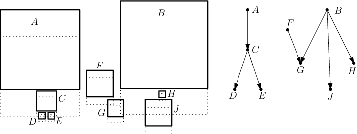
Lemma 24.

(Covering Lemma) Let $P$ be a set of $n$ points in $\mathbb{R}^{d}$ , $\kappa\in\mathbb{N}$ , and $r\in\mathbb{R}$ such that $1<r\leq n/(4(4\kappa+1)^{2d})$ . Then there is a set ${\cal K}$ of pairwise interior-disjoint cubes and a permutation of the coordinate axes such that

1.

the number of cubes is $|{\cal K}|>n/(62d\cdot(4\kappa+1)^{2d}r)$ ;
2.

for every cube $Q\in{\cal K}$ , the interior of ${\rm bott}(Q)$ contains at least $r$ points of $P$ ; and
3.

the outdegree of every node in the shift graph $T({\cal K})$ is at most one.

A permutation of the coordinate axes may be necessary, since ${\rm bott}(Q)$ and the shift graph are defined in terms of the “vertical” direction $\mathbf{e}_{d}$ .

4.1 Proof of the Covering Lemma

A cube in $\mathbb{R}^{d}$ is called a grid-cube if all coordinates of all of its vertices are integers. A unit grid-cube is a grid-cube of side length 1. A face-to-face tiling of $\mathbb{R}^{d}$ with grid-cubes is an infinite collection of pairwise interior-disjoint grid-cubes whose union is $\mathbb{R}^{d}$ such that every two grid-cubes are either disjoint or intersect in a common face. We start with a simple proposition.

Proposition 25.

Let $Q$ be a grid-cube in $\mathbb{R}^{d}$ , and let $B\subseteq Q$ be a unit grid-cube. Then $Q\setminus B$ is the union of at most $3^{d}-1$ (not necessarily disjoint) grid-cubes.

Proof.

The hyperplanes along the $2d$ sides of $B$ decompose $Q\setminus B$ into at most $3^{d}-1$ interior-disjoint axis-aligned boxes. It is enough to show that each such box can be covered by a cube lying in $Q\setminus B$ .

Consider one such box $R=\prod_{i=1}^{d}[a_{i},b_{i}]\subset Q$ . Note that all coordinates of all vertices of $R$ are integers. At least one extent of $R$ is interior-disjoint from the corresponding extent of $B$ . Assume without loss of generality that $[a_{1},b_{1}]$ is a maximal length extent of $R$ that is interior-disjoint from the corresponding extent of $B$ . Then a hyperplane $h_{1}$ orthogonal to $\mathbf{e}_{1}$ separates $R$ and $B$ (i.e., $B$ and $R$ lie in closed halfspaces on opposite sides of $h_{1}$ ). Enlarge each extent of $R$ to an interval of length $b_{1}-a_{1}$ that has integer endpoints and lies in the corresponding extent of $Q$ . We obtain a cube that contains $R$ , lies in $Q$ , and is separated from $Q$ by the hyperplane $h_{1}$ . ∎

We now state and prove a weaker version of the Covering Lemma that chooses a collection ${\cal S}$ of interior-disjoint cubes whose side-cubes jointly contain a constant fraction of the points in $P$ , but the side-cubes may have different orientations, and the condition about the shift graph is dropped.

Lemma 26.

Let $P$ be a set of $n$ points in $\mathbb{R}^{d}$ , let $\kappa\in\mathbb{N}$ , and let $r\in\mathbb{R}$ such that $1<r\leq n/(4(4\kappa+1)^{2d})$ . Then there is a set ${\cal S}$ of pairwise interior-disjoint cubes such that

1.

the number of cubes is $|{\cal S}|>n/(16(4\kappa+1)^{2d}r)$ ;
2.

for every $Q\in{\cal S}$ , the interior of a $\kappa$ -side-cube of $Q$ contains at least $r$ points of $P$ .

Proof.

We are given a set of $n$ points in $\mathbb{R}^{d}$ . We may assume, by applying a dilation if necessary, that the minimum distance between any two points in $P$ is more than $\sqrt{d}$ , the diameter of a unit cube. We may also assume, by applying a translation if necessary, that none of the coordinates of any point in $P$ is an integer.

We present a dynamic programming algorithm, Algorithm 27, that computes a collection ${\cal S}$ of cubes with the desired properties for a point set $P\subset\mathbb{R}^{d}$ . It proceeds in a finite number of phases. In phase $i\in\mathbb{N}$ , it maintains a face-to-face tiling of $\mathbb{R}^{d}$ with a set ${\cal C}_{i}$ of congruent grid-cubes. Initially, ${\cal C}_{1}$ is a tiling of $\mathbb{R}^{d}$ with unit grid-cubes. Our assumptions ensure that every unit grid-cube contains at most one point from $P$ , and every point in $P$ lies in the interior of a unit grid-cube.

In each phase $i\in\mathbb{N}$ , Algorithm 27 processes every cube of ${\cal C}_{i}$ that contains a point from $P$ , and determines a new tiling ${\cal C}_{i+1}$ . Each cube in ${\cal C}_{i+1}$ is the union of $\mu^{d}$ congruent grid-cubes from ${\cal C}_{i}$ , where $\mu=4\kappa+1$ . Algorithm 27 terminates at a phase $i\in\mathbb{N}$ , where all points of $P$ lie in a single cube of ${\cal C}_{i}$ .

We allow Algorithm 27 to delete points from $P$ , since it is enough to establish that a side-cube of each selected cube contains at least $r$ points of $P$ . The algorithm maintains a set $P_{A}\subseteq P$ of available points. Initially, $P_{A}=P$ (i.e., all points are available), but later the algorithm may delete some points from $P_{A}$ , or enclose them into special cubes (defined below).

When Algorithm 27 processes a cube $Q\in{\cal C}_{i}$ , then it may label $Q$ or some cubes contained in $Q$ as green, blue, and selected. Accordingly, we distinguish labeled and unlabeled cubes. The green labels carry information from one phase to the next, but the blue and selected labels are global (and irrevocable). At the end of the algorithm, the set of cubes labeled selected will be ${\cal S}$ . We maintain the property that every two labeled cubes are either interior-disjoint or nested. The labeled cubes are characterized as follows.

-

Green cubes. In each phase $i$ , Algorithm 27 places some cubes into the set ${\cal G}_{i}$ of green cubes. Green cubes are pairwise interior-disjoint. Every green cube contains at least $r$ points of $P$ but it does not contain any selected or blue cube. At the end of phase $i+1$ , some green cubes in ${\cal G}_{i}$ become $\kappa$ -side-cubes of selected cubes.
-

Selected cubes. Algorithm 27 incrementally places cubes into ${\cal S}$ and labels them selected. Selected cubes are interior-disjoint. Every $Q\in{\cal S}$ contains a green cube as a $\kappa$ -side-cube, and does not contain any smaller blue or selected cubes.
-

Blue cubes. Algorithm 27 builds a hierarchy of blue cubes ${\cal B}$ that enclose the selected cubes. Each blue cube contains a unique selected cube or at least two interior-disjoint blue cubes.

In every phase $i\in\mathbb{N}$ , Algorithm 27 processes all cubes in ${\cal C}_{i}$ that contain some points from $P$ , and then determines the next tiling ${\cal C}_{i+1}$ . For every tiling ${\cal C}_{i}$ , there are $\mu^{d}$ possible face-to-face tilings such that each cube in ${\cal C}_{i+1}$ contains exactly $\mu^{d}$ congruent cubes from ${\cal C}_{i}$ : Algorithm 27 chooses one of them to become ${\cal C}_{i+1}$ .

At the end of each phase $i\in\mathbb{N}$ , a cube $Q\in{\cal C}_{i}$ can be in one of the following six states. Initially, in phase $i=1$ , every cube $Q\in{\cal C}_{1}$ is in state $\mathbf{A}_{1}$ . Each state of a cube $Q\in{\cal C}_{i}$ is characterized by the labeled cubes contained in $Q$ that are maximal (for containment), and the number $|P_{A}\cap Q|$ of available points in $Q$ at the beginning of the step in which $Q$ is processed (note, however, that some of the points may be deleted from $P_{A}$ when $Q$ is processed).

$\mathbf{(A_{1})}$

$Q$ has no label, it contains no cubes from ${\cal G}_{i}\cup{\cal S}\cup{\cal B}$ , and $|P_{A}\cap Q|<r$ ;
$\mathbf{(A_{2})}$

$Q\in{\cal G}$ , $Q$ contains no cube from ${\cal S}\cup{\cal B}$ , and $r\leq|P_{A}\cap Q|<\mu^{d}r$ ;
$\mathbf{(A_{3})}$

$Q$ contains one maximal blue cube and one maximal green cube $G\in{\cal G}_{i}$ , and $|P_{A}\cap Q|<(3^{d}-1)r+(\mu^{d}-1)r<2\mu^{d}r$ ;
$\mathbf{(A_{4})}$

$Q$ has no label, $Q$ contains one maximal blue cube, and $|P_{A}\cap Q|<(3^{d}-1)r$ ;
$\mathbf{(A_{5})}$

$Q\in{\cal B}$ , $Q$ contains exactly one maximal selected cube, and $|P_{A}\cap Q|<\mu^{d}r$ ;
$\mathbf{(A_{6})}$

$Q\in{\cal B}$ , $Q$ contains at least two maximal blue cubes, and $|P_{A}\cap Q|<2\mu^{2d}r$ ;

For every cube $Q\in{\cal C}_{i}$ containing a point of $P$ , Algorithm 27 assigns $Q$ to one of the six states based on the number $|P_{A}\cap Q|$ of available points in $Q$ and the states of the $\mu^{d}$ sub-cubes of $Q$ from the previous subdivision ${\cal C}_{i-1}$ . (By default, all empty cubes in ${\cal C}_{i-1}$ are in state $\mathbf{A}_{1}$ .) We use a shorthand notation to summarize the states of all $\mu^{d}$ subcubes of a cube $Q\in{\cal C}_{i}$ . The expression $Q=\sum_{k=1}^{6}\omega_{k}\mathbf{A}_{k}$ means that $Q\in{\cal C}_{i}$ consists of $\omega_{k}$ sub-cubes from ${\cal C}_{i-1}$ in state $\mathbf{A}_{k}$ , $k=1,2,\ldots,6$ (hence $\sum_{k=1}^{6}\omega_{k}=\mu^{d}$ ). The assignment of a cube $Q$ to a state $\mathbf{A}_{k}$ is denoted by $Q\rightarrow\mathbf{A}_{k}$ .

Algorithm 27.

Input: $P\subset\mathbb{R}^{d}$ , $|P|=n$ , such that no coordinates are integers and the minimum distance between any two points is at least $\sqrt{d}$ .
$\bullet$ Set $P_{A}:=P$ , $i:=1$ , ${\cal S}:=\emptyset$ , ${\cal B}:=\emptyset$ , and ${\cal G}_{1}:=\emptyset$ . Let ${\cal C}_{1}$ be the subdivision of $\mathbb{R}^{d}$ into unit grid-cubes, each of which is in state $\mathbf{A}_{1}$ .
$\bullet$ Until all points of $P_{A}$ lie in a single cube of ${\cal C}_{i}$ in state $\mathbf{A}_{1}\cup\mathbf{A}_{4}\cup\mathbf{A}_{5}\cup\mathbf{A}_{6}$ , do:

1.

Set $i:=i+1$ , and $G_{i}=\emptyset$
2.
For every $Q\in{\cal C}_{i}$ where $Q\cap{P}\neq\emptyset$ do
1. (i)
  
  If $Q=\mu^{d}\mathbf{A}_{1}$ and $|P_{A}\cap Q|<r$ , then $Q\rightarrow\mathbf{A}_{1}$ .
2. (ii)
  
  If $Q=\mu^{d}\mathbf{A}_{1}$ and $|P_{A}\cap Q|\geq r$ , then $Q\rightarrow\mathbf{A}_{2}$ . Set ${\cal G}_{i}:={\cal G}_{i}\cup\{Q\}$ and $P_{A}:=P_{A}\setminus Q$ .
3. (iii)
  
  If $Q=(\mu^{d}-1)\mathbf{A}_{1}+\mathbf{A}_{2}$ , then $Q\rightarrow\mathbf{A}_{5}$ . Denote by $G\subset Q$ the green subcube in state $\mathbf{A}_{2}$ . $G$ is in central position within $Q$ (cf. step 4). Let $Q^{s}$ be a grid-cube lying in $Q$ such that $G={\rm bott}(Q^{s})$ . Set ${\cal S}={\cal S}\cup\{Q^{s}\}$ , ${\cal B}:={\cal B}\cup\{Q\}$ , and $P_{A}:=P_{A}\setminus Q$ .
4. (iv)
  
  If $Q=(\mu^{d}-1)\mathbf{A}_{1}+\mathbf{A}_{3}$ , then $Q\rightarrow\mathbf{A}_{6}$ . Subcube in state $\mathbf{A}_{3}$ contains a green cube $G\in{\cal G}_{i-1}$ and a maximal blue cube $B\in{\cal B}$ . The subcube in state $\mathbf{A}_{3}$ is in central position within $Q$ (cf. step 4). Let $Q^{s}\subset Q\setminus B$ be a grid-cube whose $\kappa$ -side-cube is $G$ . Set ${\cal S}:={\cal S}\cup\{Q^{s}\}$ , ${\cal B}:={\cal B}\cup\{Q,Q^{s}\}$ , and $P_{A}:=P_{A}\setminus Q$ .
5. (v)
  
  If $Q=(\mu^{d}-1)\mathbf{A}_{1}+(\mathbf{A}_{4},\mathbf{A}_{5},$ or $\mathbf{A}_{6})$ and $|P_{A}\cap Q|<(3^{d}-1)r$ , then $Q\rightarrow\mathbf{A}_{4}$ .
6. (vi)
  
  If $Q=(\mu^{d}-1)\mathbf{A}_{1}+(\mathbf{A}_{4},\mathbf{A}_{5},$ or $\mathbf{A}_{6})$ and $|P_{A}\cap Q|\geq(3^{d}-1)r$ , then $Q\rightarrow\mathbf{A}_{3}$ . Let $B$ be the maximal blue cube in $Q$ , which either lies in the subcube in state $\mathbf{A}_{4}$ or is the subcube in state $(\mathbf{A}_{5}$ or $\mathbf{A}_{6}$ ). Let $G\subset Q\setminus B$ be one of at most $3^{d}-1$ cubes covering $Q\setminus B$ (cf. Proposition 25) such that $|P_{A}\cap G|\geq r$ . Set ${\cal G}_{i}:={\cal G}_{i}\cup\{G\}$ and $P_{A}:=P_{A}\setminus G$ .
7. (vii)
  
  If $Q=(\mu^{d}-2)\mathbf{A}_{1}+\mathbf{A}_{2}+(\mathbf{A}_{4},\mathbf{A}_{5},$ or $\mathbf{A}_{6})$ , then $Q\rightarrow\mathbf{A}_{6}$ . Denote by $G$ and $B$ the subcubes of $Q$ in states $\mathbf{A}_{2}$ and $\mathbf{A}_{4}\cup\mathbf{A}_{5}\cup\mathbf{A}_{6}$ , respectively. The subcube in state $\mathbf{A}_{2}$ is in central position in $Q$ (cf. step 4). Let $Q^{s}\subset Q\setminus B$ be a grid-cube whose $\kappa$ -side-cube is $G$ . Set ${\cal B}:={\cal B}\cup\{Q,Q^{s}\}$ , ${\cal S}={\cal S}\cup\{Q^{s}\}$ , and $P_{A}:=P_{A}\setminus Q$ .
8. (viii)
  
  If $Q$ contains at least two subcubes in states ( $\mathbf{A}_{3},\mathbf{A}_{4},\mathbf{A}_{5},$ or $\mathbf{A}_{6}$ ) and the remaining subcubes are in states ( $\mathbf{A}_{1}$ or $\mathbf{A}_{2}$ ), then $Q\rightarrow\mathbf{A}_{6}$ . Set ${\cal B}:={\cal B}\cup\{Q\}$ and $P_{A}:=P_{A}\setminus Q$ .
3.

Choose ${\cal C}_{i+1}$ out of the $\mu^{d}$ possible tilings such that the maximal number of cubes in ${\cal C}_{i}$ in state $\mathbf{A}_{2}\cup\mathbf{A}_{3}$ are in central position within a cube in ${\cal C}_{i+1}$ .
4.

For every cube $Q\in{\cal C}_{i}$ in state $\mathbf{A}_{2}\cup\mathbf{A}_{3}$ that is not in central position in ${\cal C}_{i+1}$ , do: If $Q$ is in state $\mathbf{A}_{2}$ , then set ${\cal G}_{i}:={\cal G}_{i}\setminus\{Q\}$ and $Q\rightarrow\mathbf{A}_{1}$ ; if $Q$ is in state $\mathbf{A}_{3}$ containing a green cube $G\in{\cal G}_{i}$ , then set ${\cal G}_{i}:={\cal G}_{i}\setminus\{G\}$ and $Q\rightarrow\mathbf{A}_{4}$ . As a result, every surviving cube in state $\mathbf{A}_{2}\cup\mathbf{A}_{3}$ is in central position within some cube in ${\cal C}_{i+1}$ .

Output: ${\cal S}$ .

At the end of Algorithm 27, all points lie in a cube $Q$ in state $\mathbf{A}_{1}$ , $\mathbf{A}_{4}$ , $\mathbf{A}_{5}$ or $\mathbf{A}_{6}$ . Let $b$ and $s$ denote the total number of blue and selected cubes, respectively. Let $g_{i}$ denote the total number of cubes that are labeled green during phase $i$ of Algorithm 27 (even if the label was removed at the end of the phase); and let $g=\sum_{i\geq 1}g_{i}$ .

We define a rooted tree on the blue cubes as follows. The vertices of the tree correspond to the blue cubes, a cube $Q_{1}$ is a descendant of $Q_{2}$ if and only if $Q_{1}\subset Q_{2}$ . Each selected cube is contained in a unique leaf cube of this tree, and so the tree has $s$ leaves. Every intermediate node (state $\mathbf{A}_{6}$ ) has at least two children. It follows that $b<2s\leq 2b$ .

Every green cube in ${\cal G}_{i}$ is in a unique cube of ${\cal C}_{i}$ , which is in state $\mathbf{A}_{2}\cup\mathbf{A}_{3}$ . The tiling ${\cal C}_{i+1}$ was chosen such that at least $g_{i}/\mu^{d}$ cubes $Q\in{\cal C}_{i}$ in $\mathbf{A}_{2}\cup\mathbf{A}_{3}$ are in central position with respect to ${\cal C}_{i+1}$ . Each of these cubes $Q\in{\cal C}_{i}$ contains a unique green cube $G_{Q}\in{\cal G}_{i}$ . In phase $i+1$ , a green cube $G\in{\cal G}_{i}$ either becomes the $\kappa$ -side-cube of a new selected cube (cases (iii), (iv), or (vii)), or is enclosed in a new blue cube along with at least two interior-disjoint blue cubes (case (viii)). At any rate, if a cube $Q\in{\cal C}_{i}$ in state $\mathbf{A}_{2}\cup\mathbf{A}_{3}$ is in central position with respect to ${\cal C}_{i+1}$ , then $Q$ is enclosed in a unique blue cube of ${\cal C}_{i+1}$ , hence $g/\mu^{d}\leq b\leq 2s$ .

We derive an upper bound for the total number of points in terms of $s$ by accounting for the available points deleted during the algorithm. For every blue cube (in state $\mathbf{A}_{5}\cup\mathbf{A}_{6}$ ), at most $2\mu^{2d}r$ points are deleted. For every cube in state $\mathbf{A}_{2}\cup\mathbf{A}_{3}$ , at most $2\mu^{d}r$ points are deleted. Finally, at the last phase, the single remaining cube is in state $\mathbf{A}_{1}\cup\mathbf{A}_{4}\cup\mathbf{A}_{5}\cup\mathbf{A}_{6}$ , and it contains at most $2\mu^{2d}r$ available points. We have

$\displaystyle n$	$\displaystyle\leq$	$\displaystyle b\cdot 2\mu^{2d}r+g\cdot 2\mu^{d}r+2\mu^{2d}r,$
$\displaystyle n$	$\displaystyle<$	$\displaystyle 2s\cdot 2\mu^{2d}r+2\mu^{d}s\cdot 2\mu^{d}r+2\mu^{2d}r,$
$\displaystyle n-2\mu^{2d}r$	$\displaystyle<$	$\displaystyle 8\mu^{2d}r\cdot s,$
$\displaystyle\frac{n-2\mu^{2d}r}{8\mu^{2d}r}$	$\displaystyle<$	$\displaystyle s.$

The number of cubes in ${\cal S}$ is $s>(n-2\mu^{2d}r)/(8\mu^{2d}r)\geq n/(16\mu^{2d}r)$ , if $r\leq n/(4\mu^{2d})$ .∎

Proof of Lemma 24.

A $\kappa$ -side-cube of a cube in ${\cal S}$ can have $2d$ possible orientations. Let ${\cal K}_{0}$ be the set of cubes from ${\cal S}$ with the most frequent orientation. We can permute the coordinate axes such that every $\kappa$ -side-cube in ${\cal K}_{0}$ lies along the bottom sides. The cubes of ${\cal K}_{0}$ satisfy properties 1 and 2 of Lemma 24. The number of cubes in ${\cal K}_{0}$ is $|{\cal K}_{0}|=|{\cal S}|/2d>n/(32d\cdot\mu^{2d}r)$ .

We show that the indegree of every node in the shift graph $T({\cal K}_{0})$ is at most one. Assume that $(Q_{1},Q_{2})$ is a directed edge in $T({\cal K}_{0})$ . We wish to show that the indegree of $Q_{2}$ is one. Recall (Definition 23) that $(Q_{1},Q_{2})$ is an edge of $T({\cal K}_{0})$ iff (1) ${\rm shift}(Q_{1})\setminus Q_{1}$ and ${\rm shift}(Q_{2})$ overlap, and (2) there is a vertical segment connecting the bottom side of $Q_{1}$ and the top side of $Q_{2}$ that does not intersect the interior of any cube in ${\cal K}_{0}$ . Since $Q_{1}$ and $Q_{2}$ are interior-disjoint, $Q_{1}$ must be above $Q_{2}$ , and $Q_{1}$ must be larger than $Q_{2}$ .

It is enough to show that the vertical projection of $Q_{1}$ contains that of $Q_{2}$ . Indeed, suppose to the contrary, that both $(Q_{0},Q_{2})$ and $(Q_{1},Q_{2})$ are incoming edges to cube $Q_{2}$ . If the vertical projections of both $Q_{0}$ and $Q_{1}$ contain that of $Q_{2}$ , then one of $Q_{0}$ and $Q_{1}$ is above the other. Assume without loss of generality that $Q_{0}$ is above $Q_{1}$ . Then every vertical segment between $Q_{0}$ and $Q_{2}$ intersects $Q_{1}$ , contradicting property (2) of Definition 23. Therefore, the in-degree of every node in $T({\cal K}_{0})$ is at most one, as claimed.

It remains to show that the vertical projection of $Q_{1}$ contains that of $Q_{2}$ . Both $Q_{1}$ and $Q_{2}$ are in the set ${\cal S}$ of selected cubes returned by Algorithm 27. Assume without loss of generality that $Q_{1}$ was selected while processing a cube $Q_{1}^{\prime}\in{\cal C}_{i}$ in phase $i$ . Then $Q_{1}^{\prime}$ is the smallest blue cube containing $Q_{1}$ . By construction, ${\rm bott}(Q_{1})\in{\cal G}_{i-1}$ ; and ${\rm bott}(Q_{1})$ lies in a cube of ${\cal C}_{i-1}$ in state $\mathbf{A}_{2}\cup\mathbf{A}_{3}$ that is in central position within $Q_{1}^{\prime}$ . Therefore, ${\rm shift}(Q_{1})\subset Q_{1}^{\prime}$ . Since $Q_{2}$ is smaller than $Q_{1}$ and overlaps with ${\rm shift}(Q_{1})$ , we have $Q_{2}\subset Q_{1}^{\prime}$ . This implies that $Q_{1}^{\prime}$ already contains some blue cube. Hence $Q_{1}^{\prime}$ is processed in step 2iv or step 2vii of Algorithm 27. We distinguish between two cases.

Assume first that $Q_{1}^{\prime}$ is processed in step 2iv. Then $Q_{1}^{\prime}=(\mu^{d}-1)\mathbf{A}_{1}+\mathbf{A}_{3}$ , and so both ${\rm bott}(Q_{1})$ and $Q_{2}$ lie in the cube $Q_{2}^{\prime}$ in state $\mathbf{A}_{3}$ , which is in central position in $Q_{1}^{\prime}$ . Denote by $B\subset Q^{\prime}_{2}$ the maximal blue cube in $Q_{2}^{\prime}$ . The green cube ${\rm bott}(Q_{1})\subset Q_{2}^{\prime}$ was created in step 2vi of Algorithm 27, as one of at most $3^{d}-1$ cubes covering $Q\setminus B$ (cf. Proposition 25). The green cube ${\rm bott}(Q_{1})$ is one of at most $3^{d}-1$ grid-cubes covering $Q^{\prime}_{2}\setminus B$ . Since ${\rm bott}(Q_{1})$ is adjacent to the bottom side of $Q_{1}$ , and $Q_{1}$ is interior disjoint from $B$ , then ${\rm bott}(Q_{1})$ lies above the hyperplane containing the top side $B$ . By Proposition 25, the cube ${\rm bott}(Q_{1})$ is at least as large as $B$ . Since ${\rm bott}(Q_{1})$ and $B$ are adjacent, and ${\rm bott}(Q_{1})$ is a $\kappa$ -side-cube of $Q_{1}$ for $\kappa\geq 1$ , the vertical projection of $Q_{1}$ contains that of $B$ and hence that of $Q_{2}$ .

Assume now that $Q_{1}^{\prime}$ is processed in step 2vii. Then $Q_{1}^{\prime}=(\mu^{d}-2)\mathbf{A}_{1}+\mathbf{A}_{2}+(\mathbf{A}_{4},\mathbf{A}_{5},$ or $\mathbf{A}_{6})$ . The a green cube ${\rm bott}(Q_{1})$ in state $\mathbf{A}_{2}$ is in central position in $Q_{1}^{\prime}$ , and $Q_{1}$ is the union of $(2\kappa+1)^{d}$ subcubes in ${\cal C}_{i-1}$ . The cube $Q_{2}$ lies within a subcube $B^{\prime}\in{\cal C}_{i-1}$ in state $\mathbf{A}_{4}\cup\mathbf{A}_{5}\cup\mathbf{A}_{6}$ . Since $(Q_{1},Q_{2})$ is an edge of the shift graph $T({\cal K})$ , $B^{\prime}$ is one of the $(2\kappa+1)^{d-1}$ subcubes in ${\cal C}_{i-1}$ directly below $Q_{1}$ . Consequently, the vertical projection of $Q_{1}$ contains that of $B^{\prime}$ and hence that of $Q_{2}$ .

In both cases, the vertical projection of $Q_{1}$ contains the vertical projection of $Q_{2}$ , as required.

Since the indegree of every node in the shift graph $T({\cal K}_{0})$ is at most one, it follows that $T({\cal K}_{0})$ has at least $|{\cal K}_{0}|$ edges and so at least half of the nodes have outdegree 0 or 1. Let ${\cal K}$ be the set of cubes in ${\cal K}_{0}$ whose outdegree is 0 or 1 in $T({\cal K}_{0})$ . We have $|{\cal K}|\geq|{\cal K}_{0}|/2>n/(64d\cdot\mu^{2d}r)$ . This completes the proof of Lemma 24. ∎

5 Combination of the two Main Lemmas

Recall that two 2-flats in $\mathbb{R}^{4}$ that correspond to two complex lines in $\mathbb{C}^{2}$ are either parallel or intersect in a single point. We define a crossing in $\mathbb{R}^{4}$ as a pair of 2-flats in $\mathbb{R}^{4}$ that intersect in exactly one point. The Separation Lemma gives a set of points $P_{3}$ , and two sets of 2-flats in $\mathbb{R}^{4}$ , $L_{1}$ and $L_{2}$ , such that the directions of the 2-flats in $L_{1}$ and $L_{2}$ are in the $3^{\circ}$ -neighborhood of two orthogonal 2-dimensional subspaces $\hat{\ell}_{1}\in{\rm Gr}(2,2)$ and $\hat{\ell}_{2}\in{\rm Gr}(2,2)$ , respectively.

Lemmas 28 and 29 below help localizing the crossings between the lines in $L_{1}$ and $L_{2}$ . We introduce some notation for the lines incident to two specific points. Consider two points $p,q\in\mathbb{R}^{4}$ and let $d={\rm dist}(p,q)$ be their Euclidean distance. Let $\ell_{1}^{p}$ and $\ell_{2}^{p}$ (reps., $\ell_{1}^{q}$ and $\ell_{2}^{q}$ ) be two orthogonal 2-flats of direction $\hat{\ell}_{1}$ and $\hat{\ell}_{2}$ incident to $p$ (resp., $q$ ). Let $x=\ell_{1}^{p}\cap\ell_{2}^{q}$ and $y=\ell_{1}^{q}\cap\ell_{2}^{p}$ , respectively. Since $\hat{\ell}_{1}$ and $\hat{\ell}_{2}$ are orthogonal directions, $pxqy$ is a rectangle, and in particular, $p$ , $q$ , $x$ , and $y$ are coplanar in $\mathbb{R}^{4}$ .

Lemma 28.

With the above notation, the pairs of 2-flats in $L_{1}^{p}\times L_{2}^{q}$ and $L_{1}^{q}\times L_{2}^{p}$ intersect in the balls $B(x,d/10)$ and $B(y,d/10)$ of radius $\frac{d}{10}$ centered at $x$ and $y$ , respectively.

Proof.

Denote by $z=h_{1}^{p}\cap h_{2}^{q}$ the intersection point of some 2-flats $h_{1}^{p}\in L_{1}^{p}$ and $h_{2}^{q}\in L_{2}^{q}$ . Since $\ell_{1}^{p}$ and $\ell_{2}^{q}$ are orthogonal, we have $\angle pxq=90^{\circ}$ , hence $\angle pxz+\angle qxz\leq 270^{\circ}$ . Assume, without loss of generality, that $\angle pxz\leq 135^{\circ}$ (the case that $\angle qxz\leq 135^{\circ}$ is analogous). Recall that the distance between the directions of two 2-flats in $\mathbb{R}^{4}$ (i.e., the metric in ${\rm Gr}(2,2)$ ) is the sum of their principal angles. Therefore, $\angle xpz<3^{\circ}$ . In the triangle $\Delta(pxz)$ , we have $\angle pzx=180^{\circ}-\angle pxz-\angle xpz>41^{\circ}$ . By the law of sines, ${\rm dist}(x,z)={\rm dist}(p,x)\sin(\angle xpz)/\sin(\angle pzx)<d\sin 3^{\circ}/\sin 41^{\circ}<d/10$ , as claimed. ∎

Let $f$ be a hyperplane in $\mathbb{R}^{4}$ , and denote its two closed halfspaces by $f^{+}$ and $f^{-}$ , respectively. A crucial step of the argument below considers the case where two points lie on the same side of $f$ , say $p,q\in f^{+}$ , but neither $B(x,d/10)$ nor $B(y,d/10)$ is contained in $f^{+}$ . The following lemma shows that in this case, both $p$ and $q$ must be close to $f$ .

Lemma 29.

If $p,q\in f^{+}$ but neither $B(x,d/10)$ nor $B(y,d/10)$ is contained in $f^{+}$ , then both $p$ and $q$ are at distance at most $d/5$ from the hyperplane $f$ .

Proof.

Since $p,q\in f^{+}$ , the midpoint of the rectangle $pxqy$ is also in $f^{+}$ . This point is also the midpoint of $xy$ , and so at least one of $x$ and $y$ is in $f^{+}$ . Assume without loss of generality that $x\in f^{+}$ . Since $B(x,d/10)$ intersects $f^{-}$ , point $x$ is at distance at most $d/10$ from $f$ . Hence both $x$ and $y$ are at distance at most $d/10$ from $f$ (on either side of $f$ ), and the midpoint of $xy$ is also at distance at most $d/10$ from $f$ . Since $p,q\in f^{+}$ , and the midpoint of $pq$ is at distance at most $d/10$ from $f$ , both $p$ and $q$ are at distance at most $2(d/10)=d/5$ from $f$ . ∎

We combine the Separation Lemma and the Covering Lemma in the following lemma.

Lemma 30.

(Combination Lemma) Let $P$ be a set of $n$ points, and let $L_{1}$ and $L_{2}$ be two sets of 2-flats in $\mathbb{R}^{4}$ such that the directions of the 2-flats in $L_{1}$ and $L_{2}$ are in the $3^{\circ}$ -neighborhood of two orthogonal 2-dimensional subspaces $\hat{\ell}_{1}\in{\rm Gr}(2,2)$ and $\hat{\ell}_{2}\in{\rm Gr}(2,2)$ , respectively. Let $r_{0}\in\mathbb{N}$ , $1<r_{0}\leq 10^{-8}n$ .

Then there is a set ${\cal R}$ of pairwise interior-disjoint regions in $\mathbb{R}^{4}$ , and point sets $P_{R}\subset P\cap R$ for every $R\in{\cal R}$ , such that

1.

$|{\cal R}|>n/(10^{10}r_{0})$ ;
2.

$|P_{R}|=r_{0}$ for every $R\in{\cal R}$ ; and
3.

$\{e_{1}\cap e_{2}:e_{1}\in L_{1}^{p},e_{2}\in L_{2}^{q}\}\subset{\rm int}(R)$ or $\{e_{1}\cap e_{2}:e_{1}\in L_{1}^{q},e_{2}\in L_{2}^{p}\}\subset{\rm int}(R)$ for every $R\in{\cal R}$ and every $p,q\in P_{R}$ .

Proof.

Invoke the Covering Lemma (Lemma 24) for the point set $P$ with parameters $r=27r_{0}$ and $\kappa=1$ in $\mathbb{R}^{4}$ . We obtain a set ${\cal K}$ of more than $n/(64\cdot 4\cdot 5^{8}\cdot 27r_{0})>2n/(10^{10}r_{0})=2n/(Mr_{0})$ interior-disjoint cubes such that a 1-side-cube of each cube in ${\cal K}$ contains at least $27r_{0}$ points from $P$ . Assume that these special side-cubes are the lower side-cubes ${\rm bott}(Q)$ for all $Q\in{\cal K}$ (the argument is analogous for any other orientation of the side-cubes). For every cube $Q\in{\cal K}$ , we construct a region $R\in{\cal R}$ such that $Q\cap{\rm shift}(Q)\subset R$ , and choose a set $P_{R}$ of $r_{0}$ points from $P\cap{\rm bott}(Q)$ .

Consider two arbitrary points $p,q\in P\cap{\rm bott}(Q)$ , for a cube $Q\in{\cal K}$ . Let $d={\rm dist}(p,q)$ and let $x$ and $y$ be defined as above. By Lemma 28, the pairs of lines in $L_{1}^{p}\times L_{2}^{q}$ and $L_{1}^{q}\times L_{2}^{p}$ intersect in the balls $B(x,d/10)$ and $B(y,d/10)$ of radius $\frac{d}{10}$ centered at $x$ and $y$ , respectively. To establish the last condition in Lemma 30, it is enough to ensure that at least one of the balls $B(x,d/10)$ and $B(y,d/10)$ lies in the region $R$ for all $p,q\in P_{R}$ (where $x$ , $y$ , and $d$ depend on $p$ and $q$ ).

The diameter of a cube in $\mathbb{R}^{4}$ is at most twice its side length, and so $d={\rm dist}(p,q)$ is at most twice the side length of ${\rm bott}(Q)$ . It follows that both $B(x,d/10)$ and $B(y,d/10)$ are contained in ${\rm shift}(Q)$ . It is possible that for some points $p,q\in P\cap{\rm bott}(Q)$ , neither $B(x,d/10)$ nor $B(y,d/10)$ is fully contained in the interior of $Q\cap{\rm shift}(Q)$ . Therefore, region $R$ should extend below $Q$ .

We are now ready to define the regions $R\in{\cal R}$ and the point sets $P_{R}$ , $R\in{\cal R}$ . We distinguish two cases.

Case 1: $Q\in{\cal K}$ has out-degree 0 in $T({\cal K})$ . Let $R={\rm shift}(Q)$ , and let $P_{R}$ be a set of $r_{0}$ arbitrary points from $P\cap{\rm bott}(Q)$ . Properties 2 and 3 of Lemma 30 are satisfied for $R$ , in this case ${\rm shift}(Q)$ contains both balls $B(x,d/10)$ and $B(y,d/10)$ for every $p,q\in P_{R}$ .

Case 2: $Q_{1}\in{\cal K}$ has out-degree 1 in $T({\cal K})$ . Let $Q_{2}\in{\cal K}$ be the cube such that $(Q_{1},Q_{2})$ is the unique outgoing edge of $Q_{1}$ . Let $\sigma:\mathbb{R}^{4}\rightarrow f_{1}$ be the vertical projection of $\mathbb{R}^{4}$ to the horizontal hyperplane $f_{1}$ ; and denote by $\sigma(Q_{2})$ the vertical projection of $Q_{2}$ . (Fig. 5 shows the 3-dimensional analogue of the projection.) The 2-flats spanned by the 2-dimensional faces of $\sigma(Q_{2})\subset f_{1}$ decompose $\sigma(Q_{1})$ into at most 27 axis-aligned boxes. One of them, say $Q^{\prime}$ , contains the vertical projections of at least $r_{0}$ points in $P\cap{\rm bott}(Q_{1})$ . Let $B=\{p\in{\rm bott}(Q_{1}):\sigma(p)\in Q^{\prime}\}$ , and let $P_{R}$ be a set of $r_{0}$ arbitrary points in $P\cap B$ . Denote by ${\rm shift}(B)$ the translate of $B$ by vector $-\frac{h}{3}\cdot{\mathbf{e}}_{4}$ , where $h$ is the side length of $Q_{2}$ . Let region $R$ be the set of all points of $\rm{shift}(Q_{1})$ except for the points lying in or vertically below $\rm{shift}(Q_{2})$ . The regions $R\in{\cal R}$ now have pairwise disjoint interiors.

It remains to show that for every $p,q\in P_{R}$ , at least one of $B(x,d/10)$ and $B(y,d/10)$ lies in the interior of $R$ . Depending on the relative position of $Q^{\prime}$ and $\sigma(Q_{2})$ , there are $k\in\{1,2,3,4\}$ hyperplanes that contain a 3-dimensional face of $B$ and separate $B$ from $Q_{2}$ . Denote these hyperplanes by $f_{i}$ , for $i=1,\ldots,k$ , where $f_{1}$ is the horizontal hyperplane containing the bottom side of $Q_{1}$ . Denote by $f_{i}^{+}$ the halfspace bounded by $f_{i}$ that contains box $B$ (hence $B\subset\bigcup_{i=1}^{k}f_{i}^{+}$ ).

If $B(x,d/10)$ or $B(y,d/10)$ lies in the interior of $\bigcup_{i=1}^{k}f_{i}^{+}$ , then it also lies in ${\rm shift}(Q_{1})\cap(\bigcup_{i=1}^{k}f_{i}^{+})\subset R$ . Assume now that neither $B(x,d/10)$ nor $B(y,d/10)$ lies in the interior of $\bigcup_{i=1}^{k}f_{i}^{+}$ . By Lemma 29, both $p$ and $q$ are at distance at most $d/5$ from the hyperplane $f_{i}$ , for $i=1,\ldots,k$ . The intersection of the $k$ hyperplanes, $\bigcap_{i=1}^{k}f_{i}$ , is a $(4-k)$ -flat containing a face of box $B$ . On one hand, the length of the orthogonal projection of segment $pq$ to this $(4-k)$ -flat is at least $\sqrt{1-k/5^{2}}d\geq\sqrt{1-4/5^{2}}d>0.91d$ . On the other hand, the same orthogonal projection is shorter than the diameter $\sqrt{3}h$ of the 3-dimensional cube $\sigma(Q_{2})$ . We have $0.91d<\sqrt{3}h$ , hence $d/10<h/3$ . Recall that at least one of $x$ or $y$ is above the hyperplane $f_{1}$ , and so the corresponding ball, $B(x,d/10)$ or $B(y,d/10)$ , is strictly above the top side of $\rm{shift}(Q_{2})$ . It follows that $B(x,d/10)$ or $B(y,d/10)$ lies in the interior of $R$ . ∎

5.1 Proof of Theorem 1

We show that the number of point-line incidences between $n$ points and $e$ lines in $\mathbb{C}^{2}$ is at most $\max(Cn^{2/3}e^{2/3},3n,3e)$ . We proceed by contradiction. Let $(P,E)$ be a critical system of $n$ points and $e$ lines in the complex plane $\mathbb{C}^{2}$ where $n+e$ is minimal.

By the Separation Lemma, there is a set $P_{3}\subseteq P$ of at least $n/M^{8}$ points and disjoint sets of complex lines $L_{1},L_{2}\subset E$ such that for every point $p\in P_{3}$ , we have $|L_{1}^{p}|\geq I/(nM^{2})$ and $|L_{2}^{p}|\geq I/(nM^{2})$ ; and the directions of lines in $L_{1}$ and $L_{2}$ are each in a $3^{\circ}$ -neighborhood of two orthogonal directions $\hat{\ell}_{1},\hat{\ell}_{2}\in H(1,1)$ , after an appropriate nondegenerate transformation of $\mathbb{C}^{2}$ . Identify the complex plane with the four-dimensional real Euclidean space by $\tau:\mathbb{C}^{2}\longrightarrow\mathbb{R}^{4}$ . The directions of 2-flats in $\tau(L_{1})$ and $\tau(L_{2})$ are each in a $3^{\circ}$ -neighborhood of directions of two orthogonal directions $\hat{\tau}(\hat{\ell}_{2}),\hat{\tau}(\hat{\ell}_{2})\in{\rm Gr}(2,2)$ . For simplicity, we use the notation $P_{3}=\tau(P_{3})$ , $L_{1}=\tau(L_{1})$ and $L_{2}=\tau(L_{2})$ for a set of points and 2-flats in $\mathbb{R}^{4}$ . Apply Lemma 30 for $P_{3}$ , $L_{1}$ , and $L_{2}$ with parameter $r_{0}=I/(nM^{3})$ . (The constraints $1<r_{0}$ and $r_{0}\leq 10^{-8}\cdot n/M^{8}$ are satisfied by Lemma 8.) We obtain a family ${\cal R}$ of at least $|{\cal R}|>(n/M^{8})/(Mr_{0})=n/(M^{9}r_{0})$ interior-disjoint regions in $\mathbb{R}^{4}$ , and a set $P_{R}\subset P_{3}\cap R$ of exactly $r_{0}$ points for each $R\in{\cal R}$ .

We can now derive a lower bound for the number of crossings $X=\{(e_{1},e_{2})\in L_{1}\times L_{2}\}$ between the 2-flats in $L_{1}$ and $L_{2}$ . Consider a region $R\in{\cal R}$ . Each point $p\in P_{R}$ is incident to at least $I/(nM^{3})$ 2-flats in each of $L_{1}$ and $L_{2}$ . Since the 2-flats correspond to complex lines and any two points determine a unique complex line, at most $r_{0}$ 2-flats in $L_{1}^{p}$ (resp., $L_{2}^{p}$ ) may be incident to some other point in $P_{R}$ . Thus, there are at least $I/(nM^{2})-r_{0}\geq I/(2nM^{2})$ 2-flats in each of $L_{1}^{p}$ and $L_{2}^{p}$ that do not pass through any other point in $P_{R}$ . For each region $R\in{\cal R}$ , we estimate the number of crossings

X(P_{R})=\{(e_{1},e_{2})\in L_{1}\times L_{2}:\exists p,q\in P_{R}\mbox{ \rm such that }e_{1}\in L_{1}^{p},e_{2}\in L_{2}^{q},\mbox{ \rm and }e_{1}\cap e_{2}\in{\rm int}(R)\}.

By the Combination Lemma, there are at least $(I/(2nM^{2}))^{2}$ distinct crossings for each pair $p,q\in P_{R}$ . Every crossing is counted at most once, since the intersection points lie in disjoint regions of ${\cal R}$ . The total number of crossings is at least

	$\displaystyle\|X\|$	$\displaystyle\geq$	$\displaystyle\sum_{R\in{\cal R}}\|X(P_{R})\|\geq\|{\cal R}\|\cdot{r_{0}\choose 2}\left(\frac{I}{2nM^{2}}\right)^{2}>\frac{n}{M^{9}r_{0}}\cdot\frac{r_{0}^{2}}{3}\cdot\frac{I^{2}}{4n^{2}M^{4}}>$
		$\displaystyle>$	$\displaystyle\frac{r_{0}I^{2}}{nM^{14}}=\frac{I^{3}}{n^{2}M^{17}}>\frac{\max(C^{3}n^{2}e^{2},27n^{3},27e^{3})}{n^{2}M^{17}}=\frac{C^{3}n^{2}e^{2}}{n^{2}M^{17}}=\frac{C^{3}e^{2}}{M^{17}}=Me^{2},$

by Corollary 10 and $C^{3}/M^{17}=M$ (recall that $C=10^{60}$ and $M=10^{10}$ ). However, $L_{1},L_{2}\subset E$ , and so the number of crossings cannot exceed ${e\choose 2}$ . The contradicting lower and upper bounds $10^{10}e^{2}<|X|\leq{e\choose 2}$ imply that there is no critical system $(P,E)$ . We conclude that for every system of $n$ points and $e$ lines in $\mathbb{C}^{2}$ , the number of point-line incidences is bounded by $I\leq\max(Cn^{2/3}e^{2/3},3n,3e)<Cn^{2/3}e^{2/3}+3n+3e$ , as claimed.∎

References

[2] J. Beck, On the lattice property of the plane and some problems of Dirac, Motzkin and Erdős in combinatorial geometry, Combinatorica 3 (1983), 281–197.
[3] K. L. Clarkson, H. Edelsbrunner, L. Guibas, M. Sharir, and E. Welzl, Combinatorial complexity bounds for arrangements of curves and spheres, Discrete Comput. Geom. 5 (1990), 99–160.
[4] H. Edelsbrunner, Algorithms in Combinatorial Geometry, EATCS Monographs in Theoretical Computer Science, Springer, 1987.
[5] H. Edelsbrunner, L. Guibas, and M. Sharir, The complexity of many cells in three dimensional arrangements, Discrete Comput. Geom. 5 (1990), 197–216.
[6] Gy. Elekes, A combinatorial problem on polynomials, Discrete Comput. Geom. 19 (3) (1998), 383–389.
[7] Gy. Elekes, On linear combinatorics I, Concurrency—an algebraic approach, Combinatorica 17 (4) (1997), 447–458.
[8] P. Erdős, Problems and results in combinatorial geometry, in Discrete geometry and convexity (New York, 1982), vol. 440 of Ann. New York Acad. Sci., 1985, pp. 1–11.
[9] G. H. Golub and C. F. Van Loan, Matrix computations, The Johns Hopkins Univ. Press (2nd ed.), Baltimore, MD, 1989, 584–586.
[10] P. Henrici, Applied and computational complex analysis, Vol. 1, John Wiley & Sons, New York, NY, 1974, 307–314.
[11] K. Leichtweiss, Zur Riemannischen Geometrie in Grassmannschen Mannigfaltigkeiten, Math. Z. 76 (1961), 334–336.
[12] R. Narasimhan, Analysis on real and complex manifolds, Elsevier (3rd ed.), Amsterdam, 1985, pp. 66–69.
[13] J. Pach and P. K. Agarwal, Combinatorial Geometry, Wiley, New York, 1995, 180–181.
[14] J. Pach, R. Radoičić, G. Tardos, ans G. Tóth, Improving the Crossing Lemma by finding more crossings in sparse graphs, Discrete Comput. Geom. 36 (4)(2006), 527–552.
[15] J. Pach and M. Sharir, Repeated angles in the plane and related problems, J. Comb. Theory, Ser. A 59 (1) (1992), 12–22.
[16] J. Pach and M. Sharir, On the number of incidences between points and curves, Combinatorics, Probability and Computing 7 (1) (1998), 121–127.
[17] J. Pach and M. Sharir, Geometric incidences, pp. 185–224, in Towards a theory of geometric graphs, vol. 342 of Contemporary Mathematics, AMS, Providence, RI, 2004.
[18] J. Pach and G. Tóth, Graphs drawn with few crossings per edge, Combinatorica 17 (3) (1997), 427–439.
[19] J. Solymosi, On the number of sums and products, Bulletin of the London Mathematical Society 37 (4) (2005), 491–494.
[20] L. Székely, Crossing numbers and hard Erdős problems in discrete geometry, Combinatorics, Probability and Computing 6 (3) (1997), 353–358.
[21] E. Szemerédi and W. T. Trotter, Extremal problems in discrete geometry, Combinatorica 3 (1983), 381–392.
[22] E. Szemerédi and W. T. Trotter, A combinatorial distinction between the Euclidean and projective planes, European Journal of Combinatorics 4 (1983), 385–394.
[23] Y-C. Wong, Differential geometry of Grassmann manifolds, Proc. Nat. Acad. Sci. U.S.A. 47 (1967), 189–594.

The Szemerédi-Trotter Theorem in the Complex Plane

Abstract

1 Introduction

Theorem 1.

Corollaries.

Theorem 2.

Corollary 3.

Corollary 4.

Corollary 5.

Possible generalizations.

Conjecture 6.

2 Preliminaries

2.1 Outline

2.2 Grassmann manifolds

Metrics.

Embedding into Gr⁡(2,2){\rm Gr}(2,2).

Nondegenerate complex linear transformations.

3 Separation Lemma

Lemma 7.

3.1 Combinatorial preprocessing

Lemma 8.

Proof.

Corollary 9.

Corollary 10.

Lemma 11.

Proof.

3.2 Distinguishing two sets of lines

Definition 12.

Definition 13.

Lemma 14.

Proof.

3.3 Separation of two line sets

Lemma 15.

Definition 16.

Lemma 17.

Invariant 18.

Lemma 19.

Lemma 20.

Proof.

Proof of Lemma 19.

Proof of Lemma 17.

Proof of Lemma 15.

4 Covering Lemma

Definition 21.

Definition 22.

Definition 23.

Lemma 24.

4.1 Proof of the Covering Lemma

Proposition 25.

Proof.

Lemma 26.

Proof.

Algorithm 27.

Proof of Lemma 24.

5 Combination of the two Main Lemmas

Lemma 28.

Proof.

Lemma 29.

Proof.

Lemma 30.

Proof.

5.1 Proof of Theorem 1

References

Embedding into ${\rm Gr}(2,2)$ .