Minimal surfaces from circle patterns:
Geometry from combinatorics
1 Introduction
The theory of polyhedral surfaces and, more generally, the field of discrete differential geometry are presently emerging on the border of differential and discrete geometry. Whereas classical differential geometry investigates smooth geometric shapes (such as surfaces), and discrete geometry studies geometric shapes with a finite number of elements (polyhedra), the theory of polyhedral surfaces aims at a development of discrete equivalents of the geometric notions and methods of surface theory. The latter appears then as a limit of the refinement of the discretization. Current progress in this field is to a large extent stimulated by its relevance for computer graphics and visualization.
One of the central problems of discrete differential geometry is to find proper discrete analogues of special classes of surfaces, such as minimal, constant mean curvature, isothermic surfaces, etc. Usually, one can suggest various discretizations with the same continuous limit which have quite different geometric properties. The goal of discrete differential geometry is to find a discretization which inherits as many essential properties of the smooth geometry as possible.
Our discretizations are based on quadrilateral meshes, i.e. we discretize parameterized surfaces. For the discretization of a special class of surfaces, it is natural to choose an adapted parameterization. In this paper, we investigate conformal discretizations of surfaces, i.e. discretizations in terms of circles and spheres, and introduce a new discrete model for minimal surfaces. See Figs. 1 and 2. In comparison with direct methods (see, in particular, [23]), leading usually to triangle meshes, the less intuitive discretizations of the present paper have essential advantages: they respect conformal properties of surfaces, possess a maximum principle (see Remark on p. Remark), etc.


We consider minimal surfaces as a subclass of isothermic surfaces. The analogous discrete surfaces, discrete S-isothermic surfaces [4] consist of touching spheres, and of circles which intersect the spheres orthogonally in their points of contact. See Fig. 1 (right). Continuous isothermic surfaces allow a duality transformation, the Christoffel transformation. Minimal surfaces are characterized among isothermic surfaces by the property that they are dual to their Gauss map. The duality transformation and the characterization of minimal surfaces carries over to the discrete domain. Thus, one arrives at the notion of discrete minimal S-isothermic surfaces, or discrete minimal surfaces for short. The role of the Gauss maps is played by discrete S-isothermic surfaces, the spheres of which all intersect one fixed sphere orthogonally. Due to a classical theorem of Koebe (see Section 3) any 3-dimensional combinatorial convex polytope can be (essentially uniquely) realized as such a Gauss map.
This definition of discrete minimal surfaces leads to a construction method for discrete S-isothermic minimal surfaces from discrete holomorphic data, a form of a discrete Weierstrass representation (see Section 5). Moreover, the classical “associated family” of a minimal surface, which is a one-parameter family of isometric deformations preserving the Gauss map, carries over to the discrete setup (see Section 6).
Our general method to construct discrete minimal surfaces is schematically shown in the following diagram. (See also Fig.15.)
continuous minimal surface
image of curvature lines under Gauss-map
cell decomposition of (a branched cover of) the sphere
orthogonal circle pattern
Koebe polyhedron
discrete minimal surface
As usual in the theory on minimal surfaces [18], one starts constructing such a surface with a rough idea of how it should look. To use our method, one should understand its Gauss map and the combinatorics of the curvature line pattern. The image of the curvature line pattern under the Gauss map provides us with a cell decomposition of (a part of) or a covering. From these data, applying the Koebe theorem, we obtain a circle packing with the prescribed combinatorics. Finally, a simple dualization step yields the desired discrete minimal surface.
Let us emphasize that our data, besides possibly boundary conditions, are purely combinatorial—the combinatorics of the curvature line pattern. All faces are quadrilaterals and typical vertices have four edges. There may exist distinguished vertices (corresponding to the ends or umbilic points of a minimal surface) with a different number of edges.
The most nontrivial step in the above construction is the third one listed in the diagram. It is based on the Koebe theorem. It implies the existence and uniqueness for the discrete minimal S-isothermic surface under consideration, but not only this. This theorem can be made an effective tool in constructing these surfaces. For that purpose, we use a variational principle from [5], [28] for constructing circle patterns. This principle provides us with a variational description of discrete minimal S-isothermic surfaces and makes possible a solution of some Plateau problems as well.
In Section 7, we prove the convergence of discrete minimal S-isothermic surfaces to smooth minimal surfaces. The proof is based on Schramm’s approximation result for circle patterns with the combinatorics of the square grid [26]. The best known convergence result for circle patterns is -convergence of circle packings [14]. It is an interesting question whether the convergence of discrete minimal surfaces is as good.
Because of the convergence, the theory developed in this paper may be used to obtain new results in the theory of smooth minimal surfaces. A typical problem in the theory of minimal surfaces is to decide whether surfaces with some required geometric properties exist, and to construct them. The discovery of the Costa-Hoffman-Meeks surface [19], a turning point of the modern theory of minimal surfaces, was based on the Weierstrass representation. This powerful method allows the construction of important examples. On the other hand, it requires a specific study for each example; and it is difficult to control the embeddedness. Kapouleas [21] proved the existence of new embedded examples using a new method. He considers finitely many catenoids with the same axis and planes orthogonal to this axis and shows that one can desingularize the circles of intersection by deformed Scherk towers. This existence result is very intuitive, but it gives no lower bound for the genus of the surfaces. Although some examples with lower genus are known (the Costa-Hoffman-Meeks surface and generalizations [20]), proving the existence of Kapouleas’ surfaces with given genus and to construct them using conventional methods is very difficult [30]. Our method may become helpful to address these problems. At the present time, however, the construction of new minimal surfaces from discrete ones remains a challenge.
Apart from discrete minimal surfaces, there are other interesting subclasses of S-isothermic surfaces. In future publications, we plan to treat discrete constant mean curvature surfaces in Euclidean 3-space and Bryant surfaces [7], [10]. (Bryant surfaces are surfaces with constant mean curvature in hyperbolic 3-space.) Both are special subclasses of isothermic surfaces that can be characterized in terms of surface transformations. (See [4] and [16] for a definition of discrete constant mean curvature surfaces in in terms of transformations of isothermic surfaces. See [17] for the characterization of continuous Bryant surfaces in terms of surface transformations.)
More generally, we believe that the classes of discrete surfaces considered in this paper will be helpful in the development of a theory of discrete conformally parameterized surfaces.
2 Discrete S-isothermic surfaces
Every smooth immersed surface in 3-space admits curvature line parameters away from umbilic points, and every smooth immersed surface admits conformal parameters. But not every surface admits a curvature line parameterization that is at the same time conformal.
Definition 1.
A smooth immersed surface in is called isothermic if it admits a conformal curvature line parameterization in a neighborhood of every non-umbilic point.
Geometrically, this means that the curvature lines divide an isothermic surface into infinitesimal squares. An isothermic immersion (a surface patch in conformal curvature line parameters)
is characterized by the properties
| (1) |
Being an isothermic surface is a Möbius-invariant property: A Möbius transformation of Euclidean 3-space maps isothermic surfaces to isothermic surfaces. The class of isothermic surfaces contains all surfaces of revolution, all quadrics, all constant mean curvature surfaces, and, in particular, all minimal surfaces (see Theorem 4). In this paper, we are going to find a discrete version of minimal surfaces by characterizing them as a special subclass of isothermic surfaces (see Section 4).
While the set of umbilic points of an isothermic surface can in general be more complicated, we are only interested in surfaces with isolated umbilic points, and also in surfaces all points of which are umbilic. In the case of isolated umbilic points, there are exactly two orthogonally intersecting curvature lines through every non-umbilic point. An umbilic point has an even number of curvature lines originating from it, evenly spaced at angles. Minimal surfaces have isolated umbilic points. If, on the other hand, every point of the surface is umbilic, then the surface is part of a sphere (or plane) and every conformal parameterization is also a curvature line parameterization.
Definition 2 of discrete isothermic surfaces was already suggested in [3]. Roughly speaking, a discrete isothermic surface is a polyhedral surface in 3-space all faces of which are conformal squares. To make this more precise, we use the notion of a “quad-graph” to describe the combinatorics of a discrete isothermic surface, and we define “conformal square” in terms of the cross-ratio of four points in .
A cell decomposition of an oriented two-dimensional manifold (possibly with boundary) is called a quad-graph, if all its faces are quadrilaterals, that is, if they have four edges. The cross-ratio of four points , , , in the Riemann sphere is
The cross-ratio of four points in can be defined as follows: Let be a sphere (or plane) containing the four points. is unique except when the four points lie on a circle (or line). Choose an orientation on and an orientation preserving conformal map from to the Riemann sphere. The cross-ratio of the four points in is defined as the cross-ratio of the four images in the Riemann sphere. The two orientations on lead to complex conjugate cross-ratios. Otherwise, the cross-ratio does not depend on the choices involved in the definition: neither on the conformal map to the Riemann sphere, nor on the choice of when the four points lie in a circle. The cross-ratio of four points in is thus defined up to complex conjugation. (For an equivalent definition involving quaternions, see [3], [15].) The cross-ratio of four points in is invariant under Möbius transformations of . Conversely, if , , , have the same cross-ratio (up to complex conjugation) as , , , , then there is a Möbius transformation of which maps each to .
Four points in form a conformal square, if their cross-ratio is , that is, if they are Möbius-equivalent to a square. The points of a conformal square lie on a circle (see Fig. 3).

Definition 2.
Let be a quad-graph such that the degree of every interior vertex is even. (That is, every vertex has an even number of edges.) Let be the set of vertices of . A function
is called a discrete isothermic surface, if for every face of with vertices , , , in cyclic order, the points , , , form a conformal square.
The following three points should motivate this definition.
- •
Like the definition of isothermic surfaces, this definition of discrete isothermic surfaces is Möbius-invariant.
- •
- •
Interior vertices with degree different from play the role of umbilic points. At all other vertices, two edge paths—playing the role of curvature lines—intersect transversally. It is tempting to visualize a discrete isothermic surface as a polyhedral surface with planar quadrilateral faces. However, one should keep in mind that those planar faces are not Möbius invariant. On the other hand, when we will define discrete minimal surfaces as special discrete isothermic surfaces, it will be completely legitimate to view them as polyhedral surfaces with planar faces because the class of discrete minimal surfaces is not Möbius invariant anyway.
The Christoffel transformation [8] (see [15] for a modern treatment) transforms an isothermic surface into a dual isothermic surface. It plays a crucial role in our considerations. For the reader’s convenience, we provide a short proof of Proposition 1.
Proposition 1.
Let be an isothermic immersion, where is simply connected. Then the formulas
| (2) |
define (up to a translation) another isothermic immersion which is called the Christoffel transformed or dual isothermic surface.
Proof.
Remarks.
(i) In fact, the Christoffel transformation characterizes isothermic surfaces: If is an immersion and equations (2) do define another surface, then is isothermic.
(ii) The Christoffel transformation is not Möbius invariant: The dual of a Möbius transformed isothermic surface is not a Möbius transformed dual.
(iii) In equations (2), there is a minus sign in the equation for , but not in the equation for . This is an arbitrary choice. Also, a different choice of conformal curvature line parameters, this means choosing instead of , leads to a scaled dual immersion. Therefore, it makes sense to consider the dual isothermic surface as defined only up to translation and (positive or negative) scale.
The Christoffel transformation has a natural analogue in the discrete setting: In Proposition 2, we define the dual discrete isothermic surface. The basis for the discrete construction is the following Lemma. Its proof is straightforward algebra.
Lemma 1.
Suppose with
and let
where denotes the complex conjugate of . Then
Proposition 2.
Let be a discrete isothermic surface, where the quad-graph is simply connected. Then the edges of may be labelled “” and “” such that each quadrilateral has two opposite edges labelled “” and the other two opposite edges labeled “” (see Fig. 4). The dual discrete isothermic surface is defined by the formula
where denotes the difference of neighboring vertices and the sign is chosen according to the edge label.

For a consistent edge labelling to be possible, it is necessary that each vertex has an even number of edges. This condition is also sufficient if the the surface is simply connected.
In Definition 3 we define S-quad-graphs. These are specially labeled quad-graphs that are used in Definition 4 of S-isothermic surfaces. These S-isothermic surfaces form the subclass of discrete isothermic surfaces that we use to define discrete minimal surfaces in Section 4. For a discussion why S-isothermic surfaces are the right class to consider, see the Remark at the end of Section 4.
Definition 3.
An S-quad-graph is a quad-graph with interior vertices of even degree as in Definition 2 and the following additional properties (see Fig. 5):
- (i)
The 1-skeleton of is bipartite and the vertices are bi-colored “black” and “white”. (Then each quadrilateral has two black vertices and two white vertices.)
- (ii)
Interior black vertices have degree .
- (iii)
The white vertices be labeled and in such a way that each quadrilateral has one white vertex labeled and one white vertex labeled .
Definition 4.
Let be an S-quad-graph, and let be the set of black vertices. A discrete S-isothermic surface is a map
with the following properties:
- (i)
If are the neighbors of a -labeled vertex in cyclic order, then lie on a circle in in the same cyclic order. This defines a map from the -labeled vertices to the set of circles in .
- (ii)
If are the neighbors of an -labeled vertex, then lie on a sphere in . This defines a map from the -labeled vertices to the set of spheres in .
- (iii)
If and are the -labeled and the -labeled vertex of a quadrilateral of , then the circle corresponding to intersects the sphere corresponding to orthogonally.
There are two spheres through each black vertex, and the orthogonality condition (iii) of Definition 4 implies that they touch. Likewise, the two circles at a black vertex touch, i.e. they have a common tangent at the single point of intersection. Discrete S-isothermic surfaces are therefore composed of touching spheres and touching circles with spheres and circles intersecting orthogonally. Interior white vertices of degree unequal to are analogous to umbilic points of smooth isothermic surfaces. Generically, the orthogonality condition (iii) follows from the seemingly weaker condition that the two circles through a black vertex touch:

Lemma 2.
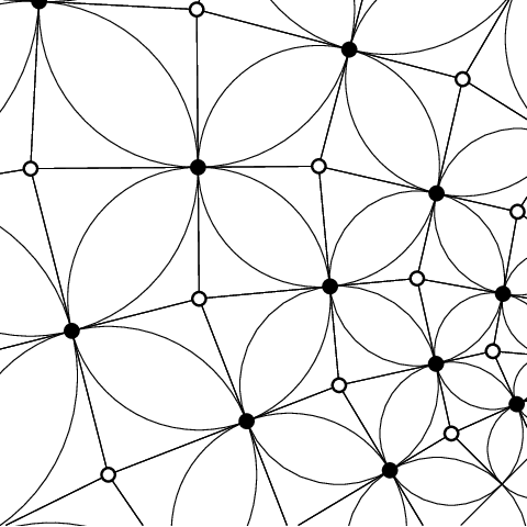
(Touching Coins Lemma) Whenever four circles in 3-space touch cyclically but do not lie on a common sphere, they intersect the sphere which passes through the points of contact orthogonally.
From any discrete S-isothermic surface, one obtains a discrete isothermic surface (as in Definition 2) by adding the centers of the spheres and circles:
Definition 5.
Let be a discrete S-isothermic surface. The central extension of is the discrete isothermic surface defined by
and otherwise
The central extension of a discrete S-isothermic surface is indeed a discrete isothermic surface: The quadrilaterals corresponding to the faces of the quad-graph are planar right-angled kites (see Fig. 3 (right)) and therefore conformal squares.
The following statement is easy to see [4]. It says that the duality transformation preserves the class of discrete S-isothermic surfaces.
Proposition 3.
The Christoffel dual of a central extension of a discrete S-isothermic surface is a central extension of a discrete S-isothermic surface.
The construction of the central extension does depend on the choice of a point at infinity, because the centers of circles and spheres are not Möbius invariant. Strictly speaking, a discrete S-isothermic surface has a -parameter family of central extensions. However, we will assume that one infinite point is chosen once and for all and we will not distinguish between S-isothermic surfaces and their central extension. Then it also makes sense to consider the S-isothermic surfaces as polyhedral surfaces. Note that all planar kites around a -labeled vertex lie in the same plane: the plane that contains the corresponding circle. We will therefore consider an S-isothermic surface as a polyhedral surface whose faces correspond to -labeled vertices of the quad-graph, whose vertices correspond to -labeled vertices of the quad-graph, and whose edges correspond to the black vertices of the quad-graph. The elements of a discrete S-isothermic surface are shown schematically in Fig. 6.
Hence:
A discrete S-isothermic surface is a polyhedral surface such that the faces have inscribed circles and the inscribed circles of neighboring faces touch their common edge in the same point.
In view of the Touching Coins Lemma (Lemma 2), this could almost be an alternative definition.
The following lemma, which follows directly from Lemma 1, describes the dual discrete S-isothermic surface in terms of the corresponding polyhedral discrete S-isothermic surface.
Lemma 3.
Let be a planar polygon with an even number of cyclically ordered edges given by the vectors , . Suppose the polygon has an inscribed circle with radius . Let be the distances from the vertices of to the nearest touching point on the circle: . Then the vectors given by
form a planar polygon with an inscribed circle with radius .
It follows that the radii of corresponding spheres and circles of a discrete S-isothermic surface and its dual are reciprocal.
3 Koebe polyhedra
In this section we construct special discrete S-isothermic surfaces, which we call the Koebe polyhedra, coming from circle packings (and more general orthogonal circle patterns) in .
A circle packing in is a configuration of disjoint discs which may touch but not intersect. Associating vertices to the discs and connecting the vertices of touching discs by edges one obtains a combinatorial representation of a circle packing, see Fig. 7 (left).


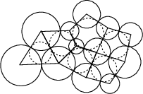
In 1936, Koebe published the following remarkable statement about circle packings in the sphere [22].
Theorem 1.
(Koebe) For every triangulation of the sphere there is a packing of circles in the sphere such that circles correspond to vertices, and two circles touch if and only if the corresponding vertices are adjacent. This circle packing is unique up to Möbius transformations of the sphere.

Observe that for a triangulation one automatically obtains not one but two orthogonally intersecting circle packings as shown in Fig. 7 (middle). Indeed, the circles passing through the points of contact of three mutually touching circles intersect these orthogonally. This observation leads to the following generalization of Koebe’s theorem to cellular decompositions of the sphere with faces which are not necessarily triangular, see Fig. 7 (right).
Theorem 2.
For every polytopal44 4 We call a cellular decomposition of a surface polytopal, if the closed cells are closed discs, and two closed cells intersect in one closed cell if at all. cellular decomposition of the sphere, there exists a pattern of circles in the sphere with the following properties. There is a circle corresponding to each face and to each vertex. The vertex circles form a packing with two circles touching if and only if the corresponding vertices are adjacent. Likewise, the face circles form a packing with circles touching if and only if the corresponding faces are adjacent. For each edge, there is a pair of touching vertex circles and a pair of touching face circles. These pairs touch in the same point, intersecting each other orthogonally.
This circle pattern is unique up to Möbius transformations.
The first published statement and proof of this theorem seems to be contained in [6]. For generalizations, see [25], [24], and [5], the latter also for a variational proof (see also Section 8 of this article).
Now, mark the centers of the circles with white dots and mark the intersection points, where two touching pairs of circles intersect each other orthogonally, with black dots. Draw edges from the center of each circle to the intersection points on its periphery. You obtain a quad-graph with bicolored vertices. Since, furthermore, the black vertices have degree four, the white vertices may be labeled and to make the quad-graph an S-quad-graph.
Now let us construct the spheres intersecting orthogonally along the circles marked by . Connecting the centers of touching spheres, one obtains a Koebe polyhedron: a convex polyhedron with all edges tangent to the sphere . Moreover, the circles marked with are inscribed into the faces of the polyhedron, see Fig. 8. Thus we have a polyhedral discrete S-isothermic surface. The discrete S-isothermic surface is given by the spheres and the circles .
Thus, Theorem 2 implies the following theorem.
Theorem 3.
Every polytopal cell decomposition of the sphere can be realized by a polyhedron with edges tangent to the sphere. This realization is unique up to projective transformations which fix the sphere.
There is a simultaneous realization of the dual polyhedron, such that corresponding edges of the dual and the original polyhedron touch the sphere in the same points and intersect orthogonally.
The last statement of the theorem follows from the construction if one interchanges the and labels.
4 Discrete minimal surfaces
The following theorem about continuous minimal surfaces is due to Christoffel [8]. For a modern treatment, see [15]. This theorem is the basis for our definition of discrete minimal surfaces. We provide a short proof for the reader’s convenience.
Theorem 4 (Christoffel).
Minimal surfaces are isothermic. An isothermic immersion is a minimal surface, if and and only if the dual immersion is contained in a sphere. In that case the dual immersion is in fact the Gauss map of the minimal surface, up to scale and translation.
Proof.
Let be an isothermic immersion with normal map . Then
where and are the principal curvature functions of and . By equations (2), the dual isothermic immersion has normal , and
Its principal curvature functions are therefore
Hence is minimal (this means ) if and only if is contained in a sphere (). In that case, is the Gauss map of (up to scale and translation), because the tangent planes of and at corresponding points are parallel. ∎
The idea is to define discrete minimal surfaces as S-isothermic surfaces which are dual to Koebe polyhedra; the latter being a discrete analogue of conformal parameterizations of the sphere. By theorem 5 below, this leads to the following definition.
Definition 6.
A discrete minimal surface is an S-isothermic discrete surface which satisfies any one of the equivalent conditions (i)–(iii) below.
Suppose is a white vertex of the quad-graph such that is the center of a sphere. Let be the vertices neighboring in . (Generically, .) Then are the points of contact with the neighboring spheres and simultaneously points of intersection with the orthogonal circles. Let . (See figure 9.) Then the following equivalent conditions hold:
- (i)
The points lie on a circle.
- (ii)
There is an such that is the same for .
- (iii)
There is plane through such that the points and the points lie in planes which are parallel to it at the same distance on opposite sides.
Remark.
The definition implies that a discrete minimal surface is a polyhedral surface with the property that every interior vertex lies in the convex hull of its neighbors. This is the maximum principle for discrete minimal surfaces.
Examples.
Fig. 1 (left) shows a discrete minimal Enneper surface. Only the circles are shown. A variant of the discrete minimal Enneper surface is shown in Fig. 16. Here, only the touching spheres are shown. Fig. 1 (right) shows a discrete minimal catenoid. Both spheres and circles are shown. Fig. 2 shows a discrete minimal Schwarz P-surface and a discrete minimal Scherk tower.
These examples are discussed in detail in section 10.
Theorem 5.
An S-isothermic discrete surface is a discrete minimal surface, if and only if the dual S-isothermic surface corresponds to a Koebe polyhedron.
Proof.
That the S-isothermic dual of a Koebe polyhedron is a discrete minimal surface is fairly obvious. On the other hand, let be a discrete minimal surface and let and be as in Definition 6. Let be the dual S-isothermic surface. We need to show that all circles of lie in one and the same sphere and that all the spheres of intersect orthogonally. It follows immediately from Definition 6 that the points lie on a circle in a sphere around . Let be the sphere which intersects orthogonally in . The orthogonal circles through also lie in . Hence, all spheres of intersect orthogonally and all circles of lie in . ∎
Remark.
Why do we use S-isothermic surfaces to define discrete minimal surfaces? Alternatively, one could define discrete minimal surfaces as the surfaces obtained by dualizing discrete (cross-ratio ) isothermic surfaces with all quad-graph vertices in a sphere. Indeed, this definition was proposed in [3]. However, it turns out that the class of discrete isothermic surfaces is too general to lead to a satisfactory theory of discrete minimal surfaces.
Every way to define the concept of a discrete isothermic immersion imposes an accompanied definition of discrete conformal maps. Since a conformal map is just an isothermic immersion into the plane, discrete conformal maps should be defined as discrete isothermic surfaces that lie in a plane. Definition 2 for isothermic surfaces implies the following definition for discrete conformal maps: A discrete conformal map is a map from a domain of to the plane such that all elementary quads have cross-ratio . The so defined discrete conformal maps are too flexible. In particular, one can fix one sublattice containing every other point and vary the other one, see [4].
Definition 4 for S-isothermic surfaces, on the other hand, leads to discrete conformal maps that are Schramm’s “circle patterns with the combinatorics of the square grid” [26]. This definition of discrete conformal maps has many advantages: First, there is Schramm’s convergence result (ibid). Secondly, orthogonal circle patterns have the right degree of rigidity. For example, by Theorem 2, two circle patterns that correspond to the same quad-graph decomposition of the sphere differ by a Möbius transformation. One could say: The only discrete conformal maps from the sphere to itself are the Möbius transformations. Finally, a conformal map is characterized by the conditions
| (3) |
To define discrete conformal maps , it is natural to impose these two conditions on two different sub-lattices (white and black) of , i.e. to require that the edges meeting at a white vertex have equal length and the edges at a black vertex meet orthogonally. Then the elementary quadrilaterals are orthogonal kites, and discrete conformal maps are therefore precisely Schramm’s orthogonal circle patterns.
5 A Weierstrass-type representation
In the classical theory of minimal surfaces, the Weierstrass representation allows the construction of an arbitrary minimal surface from holomorphic data on the underlying Riemann surface. We will now derive a formula for discrete minimal surfaces that resembles the Weierstrass representation formula. An orthogonal circle pattern in the plane plays the role of the holomorphic data. The discrete Weierstrass representation describes the S-isothermic minimal surface that is obtained by projecting the pattern stereographically to the sphere and dualizing the corresponding Koebe polyhedron.
Theorem 6 (Weierstrass representation).
Let be an S-quad-graph, and let be an orthogonal circle pattern in the plane: For white vertices , is the center of the corresponding circle, and for black vertices , is the corresponding intersection point. The S-isothermic minimal surface
that corresponds to this circle pattern is given by the following formula. Let be two vertices, both labelled , that correspond to touching circles of the pattern, and let be the black vertex between and , which corresponds to the point of contact. The centers and of the corresponding touching spheres of the S-isothermic minimal surface satisfy
| (4) |
where and the radii of the spheres are
| (5) |
The sign on the right hand side of equation (4) depends on whether the two edges of the quad-graph connecting with and with are labelled ‘’ or ‘’ (see Figs. 4 and 5 (right)).
Proof.
Let be the stereographic projection
Its differential is
and
where denotes the Euclidean norm.
The edge between and of has length (this is obvious) and is parallel to . Indeed, this edge is parallel to the corresponding edge of the Koebe polyhedron, which, in turn, is tangential to the orthogonal circles in the unit sphere, touching in . The pre-images of these circles in the plane touch in , and the contact direction is . Hence, equation (4) follows from
To show equation (5), note that the stereographic projection is the restriction of the reflection on the sphere around the north pole of with radius , restricted to the equatorial plane . See Fig. 10. We denote this reflection also by . Consider the sphere with center and radius which intersects the equatorial plane orthogonally in the circle of the planar pattern corresponding to . This sphere intersects the ray from the north pole through orthogonally at the distances from , where , the distance between and , satisfies This sphere is mapped by to a sphere, which belongs to the Koebe polyhedron and has radius . It intersects the ray orthogonally at the distances . Hence, its radius is
Equation (5) follows. ∎
6 The associated family
Every continuous minimal surfaces comes with an associated family of isometric minimal surfaces with the same Gauss map. Catenoid and helicoid are members of the same associated family of minimal surfaces. The concept of an associated family carries over to discrete minimal surfaces. In the smooth case, the members of the associated family remain conformally, but not isothermically, parameterized. Similarly, in the discrete case, one obtains discrete surfaces which are not S-isothermic but should be considered as discrete conformally parameterized minimal surfaces.
The associated family of an S-isothermic minimal surface consists of the one-parameter family of discrete surfaces that are obtained by the following construction. Before dualizing the Koebe-polyhedron (which would yield the S-isothermic minimal surface), rotate each edge by an equal angle in the plane which is tangent to the unit sphere in the point where the edge touches the unit sphere.
This construction leads to well defined surfaces because of the following lemma, which is an extension of Lemma 3. See Fig. 11.
Lemma 4.
Let be a planar polygon with an even number of cyclically ordered edges given by the vectors , . Suppose the polygon has an inscribed circle with radius , which lies in a sphere . Let be the distances from the vertices of to the nearest touching point on the circle: . Rotate each vector by an equal angle in the plane which is tangent to in the point where the edge touches the to obtain the vectors . Then the vectors given by
satisfy ; that is, they form a (non-planar) closed polygon.
Proof.
For let be the orthonormal basis of which is formed by , the unit normal to the plane of the polygon and
| (6) |
Let be the vector in the tangent plane to the sphere at that makes an angle with . Then
where is the angle between the tangent plane and the plane of the polygon. This angle is the same for all edges. Since
we have to show that
By Lemma 3,
Due to (6),
as well. Finally,
because it is a telescopic sum. ∎
The following two theorems are easy to prove. First, the Weierstrass-type formula of Theorem 6 may be extended to the associate family.
Theorem 7.
Using the notation of Theorem 6, the discrete surfaces of the associated family satisfy
Fig. 12 shows the associated family of the S-isothermic catenoid. The essential properties of the associated family of a continuous minimal surface—that the surfaces are isometric and have the same Gauss map—carries over to the discrete setting in the following form.
Theorem 8.
The surfaces of the associated family of an S-isothermic minimal surface consist, like , of touching spheres. The radii of the spheres do not depend on .
In the generic case, when the quad-graph has -combinatorics, there are also circles through the points of contact, like it is the case with . The normals of the circles do not depend on .
This theorem follows directly from the geometric construction of the associated family (Lemma 4).


7 Convergence
Schramm has proved the convergence of circle patterns with the combinatorics of the square grid to meromorphic functions [26]. Together with the Weierstrass-type representation formula for S-isothermic minimal surfaces, this implies the following approximation theorem for discrete minimal surfaces. Fig. 13 illustrates the convergence of S-isothermic Enneper surfaces to the continuous Enneper surface.
Theorem 9.
Let be a simply connected bounded domain with smooth boundary, and let be an open set that contains the closure of . Suppose that is a minimal immersion without umbilic points in conformal curvature line coordinates. There exists a sequence of S-isothermic minimal surfaces such that the following holds. Each is a simply connected S-quad-graph in which is a subset of the lattice . If, for , we define to be the value of at a point of closest to , then converges to uniformly with error on compacts in . In fact, the whole associated families converge to the associated family of uniformly (also in ) and with error on compacts in .
Proof.
Assuming that is appropriately scaled,
| (7) |
where is a locally injective meromorphic function. By Schramm’s results (Theorem 9.1 of [26] and the remark on p. 387), there exists a sequence of orthogonal circle patterns approximating and uniformly and with error on compacts in . Define by the Weierstrass formula (4) with data . Using the notation of Theorem 6, one finds
uniformly on compacts in . Setting , the convergence claim follows. The same reasoning applies to the whole associated family of . ∎


8 Orthogonal circle patterns in the sphere
In the simplest cases, like the discrete Enneper surface and the discrete catenoid (Fig. 1), the construction of the corresponding circle patterns in the sphere can be achieved by elementary methods, see Section 10. In general, the problem is not elementary. Developing methods introduced by Colin de Verdière [9], the first and third author have given a constructive proof of the generalized Koebe theorem, which uses a variational principle [5]. It also provides a method for the numerical construction of circle patterns (see also [27]). An alternative algorithm was implemented in Stephenson’s program circlepack [12]. It is based on methods developed by Thurston [29]. The first step in both methods is to transfer the problem from the sphere to the plane by a stereographic projection. Then the radii of the circles are calculated. If the radii are known, it is easy to reconstruct the circle pattern. The radii are determined by a set of nonlinear equations, and the two methods differ in the way in which these equations are solved. Thurston-type methods work by iteratively adjusting the radius of each circle so that the neighboring circles fit around. The above mentioned variational method is based on the observation that the equations for the radii are the equations for a critical point of a convex function of the radii. The variational method involves minimizing this function to solve the equations.

Both of these methods may be used to construct the circle patterns for the discrete Schwarz P-surface and for the discrete Scherk tower, see Figs. 2 and 15. One may also take advantage of the symmetries of the circle patterns and construct only a piece of it (after stereographic projection) as shown in Fig. 14. To this end, one solves the Euclidean circle pattern problem with Neumann boundary conditions: For boundary circles, the nominal angle to be covered by the neighboring circles is prescribed.
However, we have actually constructed the circle patterns for the discrete Schwarz P-surface and the discrete Scherk tower using an new method suggested in [28]. It is a variational method that works directly on the sphere. No stereographic projection is necessary; the spherical radii of the circles are calculated directly. The variational principle for spherical circle patterns is completely analogous to the variational principles for Euclidean and hyperbolic patterns presented in [5]. We briefly describe our variational method for circle patterns on the sphere. For a more detailed exposition, the reader is referred to [28]. Here, we will only treat the case of orthogonally intersecting circles.
The spherical radius of a non-degenerate circle in the unit sphere satisfies . Instead of the radii of the circles, we use the variables
| (8) |
For each circle , we need to find a such that the corresponding radii solve the circle pattern problem.
Proposition 4.
The radii are the correct radii for the circle pattern if and only if the corresponding satisfy the following equations, one for each circle:
The equation for circle is
| (9) |
where the sum is taken over all neighboring circles . For each circle , is the nominal angle covered by the neighboring circles. It is normally for interior circles, but it differs for circles on the boundary or for circles where the pattern branches.
The equations (9) are the equations for a critical point of the functional
Here, the first sum is taken over all pairs of neighboring circles, the second sum is taken over all circles . The dilogarithm function is defined by .
The second derivative of is the quadratic form
| (10) |
where the sum is taken over pairs of neighboring circles.
We provide a proof of Proposition 4 in the Appendix. Unlike the analogous functionals for euclidean and hyperbolic circle patterns, the functional is unfortunately not convex : The second derivative is negative for the tangent vector . The index is therefore at least . Thus, one cannot simply minimize to get to a critical point. However, the following method seems to work. Define a reduced functional by maximizing in the direction :
| (11) |
Obviously, is invariant under translations in the direction . Now the idea is to minimize restricted to . This method has proved to be amazingly powerful. In particular, it can be used to produce branched circle patterns in the sphere. It would be very interesting and important to give a theoretical explanation of this phenomenon.
9 Constructing discrete minimal surfaces

Gauss image of the curvature lines

circle pattern

Koebe polyhedron

discrete minimal surface
Given a specific continuous minimal surface, how does one construct an analogous discrete minimal surface? In this section we outline the general method for doing this. By way of an example, Figure 15 illustrates the construction of the Schwarz P-surface. Details on how to construct the concrete examples in this paper are explained in Section 10. The difficult part is finding the right circle pattern (paragraphs 1 and 2 below). The remaining steps, building the Koebe polyhedron and dualizing it (Paragraphs 3 and 4) are rather mechanical.
1. Investigate the Gauss image of the curvature lines.
The Gauss map of the continuous minimal surface maps its curvature lines to the sphere. Obtain a qualitative picture of this image of the curvature lines under the Gauss map. This yields a quad-graph immersed in the sphere. Here one has to choose how many curvature lines one wants to use. This corresponds to a choice of different levels of refinement of the discrete surface. Also, a choice is made as to which vertices will be black and which will be white. This choice is usually determined by the nature of the exceptional vertices corresponding to umbilics and ends. (Umbilics have to be black vertices.) Only the combinatorics of this quad graph matter. (Figure 15, top left.) Generically, the (interior) vertices have degree 4. Exceptional vertices correspond to ends and umbilic points of the continuous minimal surface. In the Figure 15, the corners of the cube are exceptional. They correspond to the umbilic points of the Schwarz P-surface. The exceptional vertices may need to be treated specially. For details see section 10.
2. Construct the circle pattern.
From the quad graph, construct the corresponding circle pattern. White vertices will correspond to circles, black vertices to intersection points. Usually, the generalized Koebe theorem is evoked to assert existence and Möbius uniqueness of the pattern. The problem of practically calculating the circle pattern was discussed in Section 8. Use symmetries of the surface or special points where you know the direction of the normal to eliminate the Möbius ambiguity of the circle pattern.
3. Construct the Koebe polyhedron.
From the circle pattern, construct the Koebe polyhedron. Here, a choice is made as to which circles will become spheres and which will become circles. The two choices lead to different discrete surfaces close to each other. Both are discrete analogues of the continuous minimal surface.
4. Discrete minimal surface.
Dualize the Koebe polyhedron to obtain a minimal surface.
If the function in the Weierstrass representation (7) of the continuous minimal surface is simple enough, it may be that one can construct an orthogonal circle pattern that is analogous to (or even approximates) this holomorphic function explicitly by some other means. For example, this is the case for the Enneper surfaces and the catenoid (see Section 9). In this case one does not use Koebe’s theorem to construct the circle pattern.
10 Examples
We now apply the method outlined in the previous section to construct concrete examples of discrete minimal surfaces. In the case of Enneper’s surface, the orthogonal circle pattern is trivial. The circle patterns for the higher order Enneper surfaces and for the catenoid are known circle pattern analogues of the functions and . To construct the circle patterns for the Schwarz P-surface and the Scherk tower, we use Koebe’s theorem.
10.1 Enneper’s surface
The Weierstrass representation of Enneper’s surface in conformal curvature line coordinates is equation (7) with . The domain is , and there are no umbilic points. In the domain, the curvature lines are the parallels to the real and imaginary axes. The Gauss map embeds the domain into the sphere.

The quad graph that captures this qualitative behavior of the curvature lines is the regular square grid decomposition of the plane. There are also obvious candidates for the circle patterns to use: Take an infinite regular square grid pattern in the plane. It consists of circles with equal radius and centers on a square grid with spacing . It was shown by He [13] that these patterns are the only embedded and locally finite orthogonal circle patterns with this quad graph. Project it stereographically to the sphere and build the Koebe polyhedron. Dualize to obtain a discrete version of Enneper’s surface. See Figs. 1 (left) and 13.
10.2 The higher order Enneper surfaces
As the next example, consider the higher order Enneper surfaces [11]. Their Weierstrass representation has . One may think of them as Enneper surfaces with an umbilic point in the center.
An orthogonal circle pattern analogue of the maps was introduced in [4]. Sectors of these circle patterns were proven to be embedded [2], [1]. Stereographic projection to the sphere followed by dualization leads to S-isothermic analogues of the higher order Enneper surfaces. An S-isothermic higher order Enneper surface with a simple umbilic point () is shown in Fig. 16.
10.3 The catenoid
The next most simple example is a discrete version of the catenoid. Here, . The corresponding circle pattern in the plane is the pattern [4], a discretization of the exponential map. The underlying quad-graph is , with circles corresponding to points with . The centers and the radii of the circles are
where
(It is not true that is an intersection point if .)
The corresponding S-isothermic minimal surface is shown in Fig. 1 (right). The associated family of the discrete catenoid (see Section 6) is shown in Fig. 12.
Other discrete versions of the catenoid have been put forward. A discrete isothermic catenoid is constructed in [3]. This construction can be generalized in such a way that one obtains the discrete S-isothermic catenoid described above. This works only because the surface is so particularly simple. Then, there is also the discrete catenoid constructed in [23]. It is an area minimizing polyhedral surface. This catenoid is not related to the S-isothermic catenoid.
10.4 The Schwarz P-surface
The Schwarz P-surface is a triply periodic minimal surface. It is the symmetric case in a -parameter family of minimal surfaces with different hole sizes (only the ratios of the hole sizes matter), see [11]. The domain of the Schwarz P-surface, where the translation periods are factored out, is a Riemann surface of genus . The Gauss map is a double cover of the sphere with branch points. The image of the curvature line pattern under the Gauss map is shown schematically in Fig. 15 (top left), thin lines. It is a refined cube. More generally, one may consider three different numbers , , and of slices in the three directions. The corners of the cube correspond to the branch points of the Gauss map. Hence, not but edges are incident with each corner vertex. The corner vertices are assigned the label . We assume that the numbers , , and are even, so that the vertices of the quad graph may be labelled ‘’, ‘’, and ‘’ consistently (see Section 2).
To invoke Koebe’s theorem (in the form of Theorem 2), forget momentarily that we are dealing with a double cover of the sphere. Koebe’s theorem implies the existence and Möbius-uniqueness of a circle pattern as shown in Fig. 15 (top right). (Only one eighth of the complete spherical pattern is shown.) The Möbius ambiguity is eliminated by imposing octahedral metric symmetry.
Now lift the circle pattern to the branched cover, construct the Koebe polyhedron and dualize it to obtain the Schwarz P-surface; see Fig. 15 (bottom row). A fundamental piece of the surface is shown in Fig. 2 (left).
We summarize these results in a theorem.
Theorem 10.
Given three even positive integers , , , there exists a corresponding unique (unsymmetric) S-isothermic Schwarz P-surface.
Surfaces with the same ratios are different discretizations of the same continuous Schwarz P-surface. The cases with correspond to the symmetric Schwarz P-surface.
10.5 The Scherk tower
Finally, consider Scherk’s saddle tower, a simply periodic minimal surface, which is asymptotic to two intersecting planes. There is a -parameter family, the parameter corresponding to the angle between the asymptotic planes, see [11]. An S-isothermic minimal Scherk tower is shown in Fig. 2 (right).
When mapped to the sphere by the Gauss map, the curvature lines of the Scherk tower form a pattern with four special points, which correspond to the four half-planar ends. A loop around a special point corresponds to a period of the surface. In a neighborhood of each special point, the pattern of curvature lines behaves like the image of the standard coordinate net under the map around . In the discrete setting, the special points are modeled by pairs of -valent vertices; see Fig. 17 (left). This is motivated by the discrete version of in [2]. The quad graph we use to construct the Scherk tower looks like the quad graph for an unsymmetric Schwarz P-surface with one of the discrete parameters equal to 2. The ratio corresponds to the parameter of the smooth case. Again, by Koebe’s theorem, there exists a corresponding circle pattern, which is made unique by imposing metric octahedral symmetry. But now we interpret the special vertices differently. Here, they are not branch points. The right hand side of Fig. 17 shows how they are to be treated: Split the vertex (and edges) between each pair of -valent vertices in two. Then introduce new -valent vertices between the doubled vertices. Thus, instead of pairs of -valent vertices we now have -valent vertices. The newly inserted edges have length . Thus, stretching the concept a little bit, one obtains infinite edges after dualization. This is in line with the fact that the special points correspond to half-planar ends.


Fig. 2 (right) shows an S-isothermic Scherk tower.
Theorem 11.
Given two even positive integers and there exists a corresponding unique S-isothermic Scherk tower.
The cases with correspond to the most symmetric Scherk tower, the asymptotic planes of which intersect orthogonally.
Appendix. Proof of Proposition 4
Figure 18 shows a “flower” of an orthogonal circle pattern: a central circle and its orthogonally intersecting neighbors. For simplicity, it shows a circle pattern in the euclidean plane. We are, however, concerned with circle patterns in the sphere, where the centers are spherical centers, the radii are spherical radii and so forth.
The radii of the circles are correct if and only if for each circle the neighboring circles “fit around”. This means that for each circle ,
where is half the angle covered by circle as seen from the center of circle , and where normally except if is a boundary circle or a circle where branching occurs. (In those cases, has some other given value.) Equations (9) follow from the following spherical trigonometry lemma:
Lemma 5.
In a right-angled spherical triangle, let and be the sides enclosing the right angle, and let be the angle opposite side . Then
| (12) |
where and are related by equation (8).
Proof.
Now let
Then a primitive function is
(see [5], [28]) and the derivative is
Since
| (14) |
one obtains after some manipulations that
This proves that Equations (9) are the equations for a critical point of .
Equation (10) for the second derivative of is obtained by taking the second derivative term by term in the first sum of equation (14). For example, the second derivative of is .
This concludes the proof of Proposition 4.
References
- [1] S. I. Agafonov, Imbedded circle patterns with the combinatorics of the square grid and discrete Painlevé equations, Discrete Comput. Geom. 29 (2003), no. 2, 305–319.
- [2] S. I. Agafonov and A. I. Bobenko, Discrete and Painlevé equations, Internat. Math. Res. Notices 2000, no. 4, 165–193.
- [3] A. I. Bobenko and U. Pinkall, Discrete isothermic surfaces, J. reine angew. Math. 475 (1996), 187–208.
- [4] A. I. Bobenko and U. Pinkall, Discretization of surfaces and integrable systems, in A. I. Bobenko and R. Seiler (eds.), Discrete Integrable Geometry and Physics, Clarendon Press, Oxford, 1999, pp. 3–58.
- [5] A. I. Bobenko and B. A. Springborn, Variational principles for circle patterns and Koebe’s theorem, Trans. Amer. Math. Soc. 356 (2004), 659–689.
- [6] G. R. Brightwell and E. R. Scheinerman, Representations of planar graphs, SIAM J. Disc. Math. 6(2) (1993), 214–229.
- [7] R. L. Bryant, Surfaces of mean curvature one in hyperbolic space, Astérisque 154–155 (1987).
- [8] E. Christoffel, Ueber einige allgemeine Eigenschaften der Minimumsflächen, J. Reine Angew. Math. 67 (1867), 218–228.
- [9] Y. Colin de Verdière, Un principe variationnel pour les empilements de cercles, Invent. Math. 104 (1991), 655–669.
- [10] P. Collin, L. Hauswirth and H. Rosenberg, The geometry of finite topology Bryant surfaces, Ann. of Math. 153 (2001), 623–659.
- [11] U. Dierkes, S. Hildebrandt, A. Küster and O. Wohlrab, Minimal Surfaces I., Springer-Verlag, Berlin, 1992.
- [12] T. Dubejko and K. Stephenson, Circle packing: Experiments in discrete analytic function theory, Experiment. Math. 4 (1995), no. 4, 307–348.
- [13] Zh. He, Rigidity of infintite disk patterns, Ann. of Math. 149 (1999), 1–33.
- [14] Zh. He and O. Schramm, The -convergence of hexagonal disk packings to the Riemann map, Acta. Math. 180 (1998), 219-245.
- [15] U. Hertrich-Jeromin, Introduction to Möbius Differential Geometry, London Mathematical Society Lecture Note Series 300, Cambridge University Press, Cambridge, 2003.
- [16] U. Hertrich-Jeromin, T. Hoffmann and U. Pinkall, A discrete version of the Darboux transform for isothermic surfaces, in A. I. Bobenko and R. Seiler (eds.), Discrete Integrable Geometry and Physics, Clarendon Press, Oxford, 1999, pp. 59–81.
- [17] U. Hertrich-Jeromin, E. Musso and N. Nicolodi, Möbius geometry of surfaces of constant mean curvature 1 in hyperbolic space, Ann. Global Anal. Geom. 19 (2001), 185–205.
- [18] D. Hoffman and H. Karcher, Complete embedded minimal surfaces of finite total curvature, in: R. Osserman (ed.), Geometry V: Minimal surfaces, Encyclopaedia of Mathematical Sciences, volume 90, Springer-Verlag, Berlin, 1997, pp. 5–93.
- [19] D. A. Hoffman and W. H. Meeks, III, A complete embedded minimal surface in with genus one an three ends, J. Differential Geom. 21 (1985) 109–127.
- [20] D. A. Hoffman and W. H. Meeks, III, Embedded minimal surfaces of finite topology, Ann. of Math. 131 (1990), no. 1, 1–34.
- [21] N. Kapouleas, Complete embedded minimal surfaces of finite total curvature, J. Differential Geom. 47 (1997), 95–169.
- [22] P. Koebe, Kontaktprobleme der konformen Abbildung, Abh. Sächs. Akad. Wiss. Leipzig Math.-Natur. Kl. 88 (1936), 141–164.
- [23] K. Polthier and W. Rossman, Discrete constant mean curvature surfaces and their index, J. reine angew. Math. 549 (2002), 47–77.
- [24] I. Rivin, A characterization of ideal polyhedra in hyperbolic 3-space, Ann. of Math. 143 (1996), 51–70.
- [25] O. Schramm, How to cage an egg, Invent. Math. 107 (1992), no. 3, 543–560.
- [26] O. Schramm, Circle patterns with the combinatorics of the square grid, Duke Math. J. 86 (1997), no. 2, 347-389.
- [27] B. A. Springborn, Constructing circle patterns using a new functional, in C. Hege and K. Polthier (eds.), Visualization and Mathematics III, Springer-Verlag, Berlin, 2003, pp. 59–68.
- [28] B. A. Springborn, Variational principles for circle patterns, PhD thesis, Technische Universität Berlin, 2003. arXiv:math.GT/0312363.
- [29] W. P. Thurston, The geometry and topology of three-manifolds, an electronic version is currently provided by the MSRI at the URL http://www.msri.org/publications/books/gt3m.
- [30] M. Weber and M. Wolf, Teichmüller theory and handle addition for minimal surfaces, Ann. of Math. 156 (2002), 713–795.
Alexander I. Bobenko
Tim Hoffmann
Boris A. Springborn
Technische Universität Berlin
Fakultät II - Institut für Mathematik
Strasse des 17. Juni 136
10623 Berlin, Germany
bobenko@math.tu-berlin.de
hoffmann@math.tu-berlin.de
springb@math.tu-berlin.de