跳到论文正文
W Papers独立论文阅读器 arXiv:math/0305169 论文正文 计算阅读时间 · 0%
引用这篇论文根据当前论文元数据生成,正式投稿前建议核对。


License: Assumed arXiv.org perpetual non-exclusive license
arXiv:math/0305169v4 [math.AT] 16 May 2005

Homological properties of non-deterministic branchings and mergings in higher dimensional automata

Philippe Gaucher Address: Preuves Programmes et Systèmes
Université Paris 7–Denis Diderot
Case 7014
2 Place Jussieu
75251 PARIS Cedex 05
France
Email address: gaucher@pps.jussieu.fr URL: http://www.pps.jussieu.fr/˜gaucher/
Abstract.

The branching (resp. merging) space functor of a flow is a left Quillen functor. The associated derived functor allows to define the branching (resp. merging) homology of a flow. It is then proved that this homology theory is a dihomotopy invariant and that higher dimensional branchings (resp. mergings) satisfy a long exact sequence.

Key words and phrases: 
concurrency, homotopy, branching, merging, homology, left Quillen functor, long exact sequence, Mayer-Vietoris, cone, higher dimensional automata, directed homotopy
1991 Mathematics Subject Classification
55P99, 68Q85

1. Introduction

The category of flows [Gau03] is an algebraic topological model of higher dimensional automata [Pra91] [Gla04]. Two kinds of mathematical problems are particularly of importance for such objects: 1) reducing the size of the category of flows by the introduction of a class of dihomotopy equivalences identifying flows having the same computer-scientific properties ; 2) investigating the mathematical properties of these dihomotopy equivalences for instance by constructing related model category structures and algebraic invariants. For other examples of similar investigations with different algebraic topological models of concurrency, cf. for example [Gra03] [Bub04] [Gou03].

This paper is concerned with the second kind of mathematical problems. Indeed, the purpose of this work is the construction of two dihomotopy invariants, the branching homology H∗−​(X)H_{*}^{-}(X) and the merging homology H∗+​(X)H_{*}^{+}(X) of a flow XX, detecting the non-deterministic branching areas (resp. merging areas) of non-constant execution paths in the higher dimensional automaton modelled by the flow XX. Dihomotopy invariance means in the framework of flows invariant with respect to weak S-homotopy (Corollary 6.5) and with respect to T-homotopy (Proposition 7.4).

The core of the paper is focused on the case of branchings. The case of mergings is similar and is postponed to Appendix A.

The branching space of a flow is introduced in Section 3 after some reminders about flows themselves in Section 2. Loosely speaking, the branching space of a flow is the space of germs of non-constant execution paths beginning in the same way. This functor is the main ingredient in the construction of the branching homology.

However it is badly behaved with respect to weak S-homotopy equivalences, as proved in Section 4. Therefore it cannot be directly used for the construction of a dihomotopy invariant. This problem is overcome in Section 5 by introducing the homotopy branching space of a flow: compare Theorem 4.1 and Corollary 5.7. The link between the homotopy branching space and the branching space is that they coincide up to homotopy for cofibrant flows, and the latter are the only interesting and real examples (Proposition 9.1).

Using this new functor, the branching homology is finally constructed in Section 6 and it is proved in the same section and in Section 7 that it is a dihomotopy invariant (Corollary 6.5 and Proposition 7.4).

Section 8 uses the previous construction to establish the following long exact sequence for higher dimensional branchings:

Theorem.

For any morphism of flows f:X⟶Yf:X\longrightarrow Y, one has the long exact sequence

…→Hn−​(X)→Hn−​(Y)→Hn−​(C​f)→…\displaystyle\dots\rightarrow H_{n}^{-}(X)\rightarrow H_{n}^{-}(Y)\rightarrow H_{n}^{-}(Cf)\rightarrow\dots
…→H3−​(X)→H3−​(Y)→H3−​(C​f)→\displaystyle\dots\rightarrow H_{3}^{-}(X)\rightarrow H_{3}^{-}(Y)\rightarrow H_{3}^{-}(Cf)\rightarrow
H2−​(X)→H2−​(Y)→H2−​(C​f)→\displaystyle H_{2}^{-}(X)\rightarrow H_{2}^{-}(Y)\rightarrow H_{2}^{-}(Cf)\rightarrow
H0​(ho​ℙ−⁡X)→H0​(ho​ℙ−⁡Y)→H0​(ho​ℙ−⁡Cf)→0.\displaystyle H_{0}(\hop^{-}X)\rightarrow H_{0}(\hop^{-}Y)\rightarrow H_{0}(\hop^{-}Cf)\rightarrow 0.

where C​fCf is the cone of ff and where H0​(ho​ℙ−⁡Z)H_{0}(\hop^{-}Z) is the free abelian group generated by the path-connected components of the homotopy branching space of the flow ZZ.

By now, this homological result does not have any known computer scientific interpretation. But it sheds some light on the potential of an algebraic topological approach of concurrency.

At last, Section 9 then gives several examples of calculation which illustrate the mathematical notions presented here.

Appendix B is a technical section which proves that two S-homotopy equivalent flows (which are not necessary cofibrant) have homotopy equivalent branching spaces. The result is not useful at all for the core of the paper but is interesting enough to be presented in an appendix of a paper devoted to branching homology.

Some familiarity with model categories is required for a good understanding of this work. However some reminders are included in this paper. Possible references for model categories are [Hov99], [Hir03] and [DS95]. The original reference is [Qui67].

2. The category of flows

In this paper, 𝐓𝐨𝐩{\rm{\mathbf{Top}}} is the category of compactly generated topological spaces, i.e. of weak Hausdorff kk-spaces (cf. [Bro88], [May99] and the appendix of [Lew78]).

Definition 2.1.

Let i:A⟶Bi:A\longrightarrow B and p:X⟶Yp:X\longrightarrow Y be maps in a category 𝒞\mathcal{C}. Then ii has the left lifting property (LLP) with respect to pp (or pp has the right lifting property (RLP) with respect to ii) if for any commutative square

A\textstyle{A\ignorespaces\ignorespaces\ignorespaces\ignorespaces\ignorespaces\ignorespaces\ignorespaces\ignorespaces}i\scriptstyle{i}α\scriptstyle{\alpha}X\textstyle{X\ignorespaces\ignorespaces\ignorespaces\ignorespaces}p\scriptstyle{p}B\textstyle{B\ignorespaces\ignorespaces\ignorespaces\ignorespaces\ignorespaces\ignorespaces\ignorespaces\ignorespaces}g\scriptstyle{g}β\scriptstyle{\beta}Y\textstyle{Y}

there exists gg making both triangles commutative.

The category 𝐓𝐨𝐩{\rm{\mathbf{Top}}} is equipped with the unique model structure having the weak homotopy equivalences as weak equivalences and having the Serre fibrations 11 1 that is a continuous map having the RLP with respect to the inclusion 𝐃n×0⊂𝐃n×[0,1]\mathbf{D}^{n}\times 0\subset\mathbf{D}^{n}\times[0,1] for any n⩾0n\geqslant 0 where 𝐃n\mathbf{D}^{n} is the nn-dimensional disk as fibrations.

Definition 2.2.

[Gau03] A flow XX consists of a compactly generated topological space ℙ​X\mathbb{P}X, a discrete space X0X^{0}, two continuous maps ss and tt called respectively the source map and the target map from ℙ​X\mathbb{P}X to X0X^{0} and a continuous and associative map ∗:{(x,y)∈ℙ​X×ℙ​X;t⁡(x)=s⁡(y)}⟶ℙ​X*:\{(x,y)\in\mathbb{P}X\times\mathbb{P}X;t(x)=s(y)\}\longrightarrow\mathbb{P}X such that s⁡(x∗y)=s⁡(x)s(x*y)=s(x) and t⁡(x∗y)=t⁡(y)t(x*y)=t(y). A morphism of flows f:X⟶Yf:X\longrightarrow Y consists of a set map f0:X0⟶Y0f^{0}:X^{0}\longrightarrow Y^{0} together with a continuous map ℙ​f:ℙ​X⟶ℙ​Y\mathbb{P}f:\mathbb{P}X\longrightarrow\mathbb{P}Y such that f⁡(s⁡(x))=s⁡(f⁡(x))f(s(x))=s(f(x)), f⁡(t⁡(x))=t⁡(f⁡(x))f(t(x))=t(f(x)) and f⁡(x∗y)=f⁡(x)∗f⁡(y)f(x*y)=f(x)*f(y). The corresponding category is denoted by 𝐅𝐥𝐨𝐰{\rm{\mathbf{Flow}}}.

The topological space X0X^{0} is called the 00-skeleton of XX. The elements of the 00-skeleton X0X^{0} are called states or constant execution paths. The elements of ℙ​X\mathbb{P}X are called non-constant execution paths. An initial state (resp. a final state) is a state which is not the target (resp. the source) of any non-constant execution path. The initial flow is denoted by ∅\varnothing. The terminal flow is denoted by 𝟏\mathbf{1}. The initial flow ∅\varnothing is of course the unique flow such that ∅0=ℙ​∅=∅\varnothing^{0}=\mathbb{P}\varnothing=\varnothing (the empty set). The terminal flow is defined by 𝟏0={0}\mathbf{1}^{0}=\{0\}, ℙ​𝟏={u}\mathbb{P}\mathbf{1}=\{u\} and the composition law u∗u=uu*u=u.

Notation 2.3.

[Gau03] For α,β∈X0\alpha,\beta\in X^{0}, let ℙα,β​X\mathbb{P}_{\alpha,\beta}X be the subspace of ℙ​X\mathbb{P}X equipped with the Kelleyfication of the relative topology consisting of the non-constant execution paths γ\gamma of XX with beginning s⁡(γ)=αs(\gamma)=\alpha and with ending t⁡(γ)=βt(\gamma)=\beta.

Several examples of flows are presented in Section 9. But two examples are important for the sequel:

Definition 2.4.

[Gau03] Let ZZ be a topological space. Then the globe of ZZ is the flow Glob⁡(Z){\rm{Glob}}(Z) defined as follows: Glob​(Z)0={0,1}{\rm{Glob}}(Z)^{0}=\{0,1\}, ℙ​Glob​(Z)=Z\mathbb{P}{\rm{Glob}}(Z)=Z, s=0s=0, t=1t=1 and the composition law is trivial. The mapping Glob:𝐓𝐨𝐩⟶𝐅𝐥𝐨𝐰{\rm{Glob}}:{\rm{\mathbf{Top}}}\longrightarrow{\rm{\mathbf{Flow}}} gives rise to a functor in an obvious way.

Refer to caption
Figure 1. Symbolic representation of Glob⁡(X){\rm{Glob}}(X) for some topological space XX
Notation 2.5.

[Gau03] If ZZ and TT are two topological spaces, then the flow

Glob⁡(Z)∗Glob⁡(T){\rm{Glob}}(Z)*{\rm{Glob}}(T)

is the flow obtained by identifying the final state of Glob⁡(Z){\rm{Glob}}(Z) with the initial state of Glob⁡(T){\rm{Glob}}(T). In other terms, one has the pushout of flows:

{0}\textstyle{\{0\}\ignorespaces\ignorespaces\ignorespaces\ignorespaces\ignorespaces\ignorespaces\ignorespaces\ignorespaces}0↦1\scriptstyle{0\mapsto 1}0↦0\scriptstyle{0\mapsto 0}Glob⁡(Z)\textstyle{{\rm{Glob}}(Z)\ignorespaces\ignorespaces\ignorespaces\ignorespaces}Glob⁡(T)\textstyle{{\rm{Glob}}(T)\ignorespaces\ignorespaces\ignorespaces\ignorespaces}Glob⁡(Z)∗Glob⁡(T)\textstyle{\ignorespaces\ignorespaces\ignorespaces\ignorespaces\ignorespaces\ignorespaces\ignorespaces\ignorespaces{\rm{Glob}}(Z)*{\rm{Glob}}(T)}

3. The branching space of a flow

Loosely speaking, the branching space of a flow is the space of germs of non-constant execution paths beginning in the same way.

Proposition 3.1.

Let XX be a flow. There exists a topological space ℙ−​X\mathbb{P}^{-}X unique up to homeomorphism and a continuous map h−:ℙ​X⟶ℙ−​Xh^{-}:\mathbb{P}X\longrightarrow\mathbb{P}^{-}X satisfying the following universal property:

  1. (1)

    For any xx and yy in ℙ​X\mathbb{P}X such that t⁡(x)=s⁡(y)t(x)=s(y), the equality h−​(x)=h−​(x∗y)h^{-}(x)=h^{-}(x*y) holds.

  2. (2)

    Let ϕ:ℙ​X⟶Y\phi:\mathbb{P}X\longrightarrow Y be a continuous map such that for any xx and yy of ℙ​X\mathbb{P}X such that t⁡(x)=s⁡(y)t(x)=s(y), the equality ϕ⁡(x)=ϕ⁡(x∗y)\phi(x)=\phi(x*y) holds. Then there exists a unique continuous map ϕ¯:ℙ−​X⟶Y\overline{\phi}:\mathbb{P}^{-}X\longrightarrow Y such that ϕ=ϕ¯∘h−\phi=\overline{\phi}\circ h^{-}.

Moreover, one has the homeomorphism

ℙ−​X≅⨆α∈X0ℙα−​X\mathbb{P}^{-}X\cong\bigsqcup_{\alpha\in X^{0}}\mathbb{P}^{-}_{\alpha}X

where ℙα−​X:=h−​(⨆β∈X0ℙα,β−​X)\mathbb{P}^{-}_{\alpha}X:=h^{-}\left(\bigsqcup_{\beta\in X^{0}}\mathbb{P}^{-}_{\alpha,\beta}X\right). The mapping X↦ℙ−​XX\mapsto\mathbb{P}^{-}X yields a functor ℙ−\mathbb{P}^{-} from 𝐅𝐥𝐨𝐰{\rm{\mathbf{Flow}}} to 𝐓𝐨𝐩{\rm{\mathbf{Top}}}.

Proof.

Consider the intersection of all equivalence relations whose graph is closed in ℙ​X×ℙ​X\mathbb{P}X\times\mathbb{P}X and containing the pairs (x,x∗y)(x,x*y) for any x∈ℙ​Xx\in\mathbb{P}X and any y∈ℙ​Xy\in\mathbb{P}X such that t⁡(x)=s⁡(y)t(x)=s(y): one obtains an equivalence relation ℛ−\mathcal{R}^{-}. The quotient ℙ​X/ℛ−\mathbb{P}X/\mathcal{R}^{-} equipped with the final topology is still a kk-space since the colimit is the same in the category of kk-spaces and in the category of general topological spaces, and is weak Hausdorff as well since the diagonal of ℙ​X/ℛ−\mathbb{P}X/\mathcal{R}^{-} is closed in ℙ​X/ℛ−×ℙ​X/ℛ−\mathbb{P}X/\mathcal{R}^{-}\times\mathbb{P}X/\mathcal{R}^{-}. Let ϕ:ℙ​X⟶Y\phi:\mathbb{P}X\longrightarrow Y be a continuous map such that for any xx and yy of ℙ​X\mathbb{P}X with t⁡(x)=s⁡(y)t(x)=s(y), the equality ϕ⁡(x)=ϕ⁡(x∗y)\phi(x)=\phi(x*y) holds. Then the equivalence relation on ℙ​X\mathbb{P}X defined by “xx equivalent to yy if and only if ϕ⁡(x)=ϕ⁡(y)\phi(x)=\phi(y)” has a closed graph which contains the graph of ℛ−\mathcal{R}^{-}. Hence the remaining part of the statement. ∎

Definition 3.2.

Let XX be a flow. The topological space ℙ−​X\mathbb{P}^{-}X is called the branching space of the flow XX. The functor ℙ−\mathbb{P}^{-} is called the branching space functor.

4. Bad behaviour of the branching space functor

The purpose of this section is the proof of the following fact:

Theorem 4.1.

There exists a weak S-homotopy equivalence of flows f:X⟶Yf:X\longrightarrow Y such that the topological spaces ℙ−​X\mathbb{P}^{-}X and ℙ−​Y\mathbb{P}^{-}Y are not weakly homotopy equivalent.

In other terms, the branching space functor alone is not appropriate for the construction of dihomotopy invariants.

Lemma 4.2.

Let ZZ be a flow such that Z0={α,β,γ}Z^{0}=\{\alpha,\beta,\gamma\} and such that ℙ​Z=ℙα,β​Z⊔ℙβ,γ​Z⊔ℙα,γ​Z\mathbb{P}Z=\mathbb{P}_{\alpha,\beta}Z\sqcup\mathbb{P}_{\beta,\gamma}Z\sqcup\mathbb{P}_{\alpha,\gamma}Z. Such a flow ZZ is entirely characterized by the three topological spaces ℙα,β​Z\mathbb{P}_{\alpha,\beta}Z, ℙβ,γ​Z\mathbb{P}_{\beta,\gamma}Z and ℙα,γ​Z\mathbb{P}_{\alpha,\gamma}Z and the continuous map ℙα,β​Z×ℙβ,γ​Z⟶ℙα,γ​Z\mathbb{P}_{\alpha,\beta}Z\times\mathbb{P}_{\beta,\gamma}Z\longrightarrow\mathbb{P}_{\alpha,\gamma}Z. Moreover, one has the pushout of topological spaces

ℙα,β​Z×ℙβ,γ​Z\textstyle{\mathbb{P}_{\alpha,\beta}Z\times\mathbb{P}_{\beta,\gamma}Z\ignorespaces\ignorespaces\ignorespaces\ignorespaces\ignorespaces\ignorespaces\ignorespaces\ignorespaces}∗\scriptstyle{*}ℙα,γ​Z\textstyle{\mathbb{P}_{\alpha,\gamma}Z\ignorespaces\ignorespaces\ignorespaces\ignorespaces}ℙα,β​Z\textstyle{\mathbb{P}_{\alpha,\beta}Z\ignorespaces\ignorespaces\ignorespaces\ignorespaces}ℙα−​Z\textstyle{\ignorespaces\ignorespaces\ignorespaces\ignorespaces\ignorespaces\ignorespaces\ignorespaces\ignorespaces\mathbb{P}_{\alpha}^{-}Z}

and the isomorphisms of topological spaces ℙβ−​Z≅ℙβ,γ​Z\mathbb{P}_{\beta}^{-}Z\cong\mathbb{P}_{\beta,\gamma}Z and ℙ−​Z≅ℙα−​Z⊔ℙβ−​Z\mathbb{P}^{-}Z\cong\mathbb{P}_{\alpha}^{-}Z\sqcup\mathbb{P}_{\beta}^{-}Z.

Proof.

It suffices to check that the universal property of Proposition 3.1 is satisfied by ℙ−​Z\mathbb{P}^{-}Z. ∎

For n⩾1n\geqslant 1, let 𝐃n\mathbf{D}^{n} be the closed nn-dimensional disk and let 𝐒n−1\mathbf{S}^{n-1} be its boundary. Let 𝐃0={0}\mathbf{D}^{0}=\{0\}. Let 𝐒−1=∅\mathbf{S}^{-1}=\varnothing be the empty space.

Refer to caption
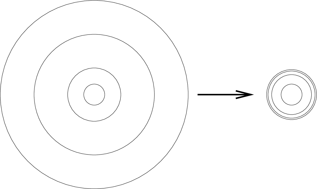
Figure 2. ‖ϕ⁡(x,y)‖=x2+y21+x2+y2||\phi(x,y)||=\frac{\sqrt{x^{2}+y^{2}}}{1+\sqrt{x^{2}+y^{2}}}

Let XX and YY be the flows defined as follows:

  1. (1)

    X0=Y0={α,β,γ}X^{0}=Y^{0}=\{\alpha,\beta,\gamma\}

  2. (2)

    ℙα,β​X=ℙβ,γ​X={0}\mathbb{P}_{\alpha,\beta}X=\mathbb{P}_{\beta,\gamma}X=\{0\}

  3. (3)

    ℙα,β​Y=ℙβ,γ​Y=ℝ\mathbb{P}_{\alpha,\beta}Y=\mathbb{P}_{\beta,\gamma}Y=\mathbb{R}

  4. (4)

    ℙα,γ​X=ℙα,γ​Y=𝐒2\mathbb{P}_{\alpha,\gamma}X=\mathbb{P}_{\alpha,\gamma}Y=\mathbf{S}^{2}

  5. (5)

    the composition law ℙα,β​X×ℙβ,γ​X⟶ℙα,γ​X\mathbb{P}_{\alpha,\beta}X\times\mathbb{P}_{\beta,\gamma}X\longrightarrow\mathbb{P}_{\alpha,\gamma}X is given by the constant map (0,0)↦(0,0,1)∈𝐒2(0,0)\mapsto(0,0,1)\in\mathbf{S}^{2}

  6. (6)

    the composition law ℙα,β​Y×ℙβ,γ​Y⟶ℙα,γ​Y\mathbb{P}_{\alpha,\beta}Y\times\mathbb{P}_{\beta,\gamma}Y\longrightarrow\mathbb{P}_{\alpha,\gamma}Y is given by the composite

    ℝ×ℝ\textstyle{\mathbb{R}\times\mathbb{R}\ignorespaces\ignorespaces\ignorespaces\ignorespaces}ϕ\scriptstyle{\phi}𝐃2\𝐒1\textstyle{\mathbf{D}^{2}\backslash\mathbf{S}^{1}\ignorespaces\ignorespaces\ignorespaces\ignorespaces}𝐃2⊔𝐒1{(1,0,0)}≅𝐒2\textstyle{\mathbf{D}^{2}\sqcup_{\mathbf{S}^{1}}\{(1,0,0)\}\cong\mathbf{S}^{2}}

    where ϕ\phi is the homeomorphism (cf. Figure 2) defined by

    ϕ⁡(x,y)=(x1+x2+y2,y1+x2+y2)\phi(x,y)=\left(\frac{x}{1+\sqrt{x^{2}+y^{2}}},\frac{y}{1+\sqrt{x^{2}+y^{2}}}\right)

Then one has the pushouts of compactly generated topological spaces

{0}×{0}\textstyle{\{0\}\times\{0\}\ignorespaces\ignorespaces\ignorespaces\ignorespaces\ignorespaces\ignorespaces\ignorespaces\ignorespaces}𝐒2\textstyle{\mathbf{S}^{2}\ignorespaces\ignorespaces\ignorespaces\ignorespaces}{0}\textstyle{\{0\}\ignorespaces\ignorespaces\ignorespaces\ignorespaces}ℙα−​X\textstyle{\ignorespaces\ignorespaces\ignorespaces\ignorespaces\ignorespaces\ignorespaces\ignorespaces\ignorespaces\mathbb{P}_{\alpha}^{-}X}

and

ℝ×ℝ\textstyle{\mathbb{R}\times\mathbb{R}\ignorespaces\ignorespaces\ignorespaces\ignorespaces\ignorespaces\ignorespaces\ignorespaces\ignorespaces}𝐒2\textstyle{\mathbf{S}^{2}\ignorespaces\ignorespaces\ignorespaces\ignorespaces}ℝ\textstyle{\mathbb{R}\ignorespaces\ignorespaces\ignorespaces\ignorespaces}ℙα−​Y\textstyle{\ignorespaces\ignorespaces\ignorespaces\ignorespaces\ignorespaces\ignorespaces\ignorespaces\ignorespaces\mathbb{P}_{\alpha}^{-}Y}
Lemma 4.3.

One has the pushout of compactly generated topological spaces

ℝ×ℝ\textstyle{\mathbb{R}\times\mathbb{R}\ignorespaces\ignorespaces\ignorespaces\ignorespaces\ignorespaces\ignorespaces\ignorespaces\ignorespaces}𝐃2⊔𝐒1{(1,0,0)}≅𝐒2\textstyle{\mathbf{D}^{2}\sqcup_{\mathbf{S}^{1}}\{(1,0,0)\}\cong\mathbf{S}^{2}\ignorespaces\ignorespaces\ignorespaces\ignorespaces}ℝ\textstyle{\mathbb{R}\ignorespaces\ignorespaces\ignorespaces\ignorespaces}{(1,0,0)}\textstyle{\{(1,0,0)\}\ignorespaces\ignorespaces\ignorespaces\ignorespaces\ignorespaces\ignorespaces\ignorespaces\ignorespaces}
Proof.

Let k​𝐓𝐨𝐩k{\rm{\mathbf{Top}}} be the category of kk-spaces. It is well known that the inclusion functor i:𝐓𝐨𝐩⟶k​𝐓𝐨𝐩i:{\rm{\mathbf{Top}}}\longrightarrow k{\rm{\mathbf{Top}}} has a left adjoint w:k​𝐓𝐨𝐩⟶𝐓𝐨𝐩w:k{\rm{\mathbf{Top}}}\longrightarrow{\rm{\mathbf{Top}}} such that w∘i=Id𝐓𝐨𝐩w\circ i=\id_{\rm{\mathbf{Top}}}. So, first of all, one has to calculate the pushout in the category of kk-spaces:

ℝ×ℝ\textstyle{\mathbb{R}\times\mathbb{R}\ignorespaces\ignorespaces\ignorespaces\ignorespaces\ignorespaces\ignorespaces\ignorespaces\ignorespaces}𝐃2⊔𝐒1{(1,0,0)}≅𝐒2\textstyle{\mathbf{D}^{2}\sqcup_{\mathbf{S}^{1}}\{(1,0,0)\}\cong\mathbf{S}^{2}\ignorespaces\ignorespaces\ignorespaces\ignorespaces}ℝ\textstyle{\mathbb{R}\ignorespaces\ignorespaces\ignorespaces\ignorespaces}X\textstyle{X\ignorespaces\ignorespaces\ignorespaces\ignorespaces\ignorespaces\ignorespaces\ignorespaces\ignorespaces}

and then, one has to prove that {(1,0,0)}≅w⁡(X)\{(1,0,0)\}\cong w(X).

Colimits in k​𝐓𝐨𝐩k{\rm{\mathbf{Top}}} are calculated by taking the colimit of the underlying diagram of sets and by endowing the result with the final topology. The colimit of the underlying diagram of sets is exactly the disjoint sum ℝ⊔{(1,0,0)}\mathbb{R}\sqcup\{(1,0,0)\}. A subset Ω\Omega of ℝ⊔{(1,0,0)}\mathbb{R}\sqcup\{(1,0,0)\} is open for the final topology if and only its inverse images in ℝ\mathbb{R} and 𝐒2\mathbf{S}^{2} are both open. The inverse image of Ω\Omega in ℝ\mathbb{R} is exactly Ω\{(1,0,0)}\Omega\backslash\{(1,0,0)\}. The inverse image of Ω\Omega in ℝ×ℝ\mathbb{R}\times\mathbb{R} is exactly Ω\{(1,0,0)}×ℝ\Omega\backslash\{(1,0,0)\}\times\mathbb{R}. Therefore the inverse image of Ω\Omega in 𝐒2\mathbf{S}^{2} is equal to ϕ⁡(Ω\{(1,0,0)}×ℝ)\phi(\Omega\backslash\{(1,0,0)\}\times\mathbb{R}) if (1,0,0)∉Ω(1,0,0)\notin\Omega, and is equal to ϕ⁡(Ω\{(1,0,0)}×ℝ)∪{(1,0,0)}\phi(\Omega\backslash\{(1,0,0)\}\times\mathbb{R})\cup\{(1,0,0)\} if (1,0,0)∈Ω(1,0,0)\in\Omega. Therefore, there are now two mutually exclusive cases:

  1. (1)

    (1,0,0)∉Ω(1,0,0)\notin\Omega; in this case, Ω\Omega is open if and only if it is open in ℝ\mathbb{R}

  2. (2)

    (1,0,0)∈Ω(1,0,0)\in\Omega; in that case, Ω\Omega is open if and only if Ω\{(1,0,0)}\Omega\backslash\{(1,0,0)\} is open in ℝ\mathbb{R} and ϕ⁡(Ω\{(1,0,0)}×ℝ)∪{(1,0,0)}\phi(\Omega\backslash\{(1,0,0)\}\times\mathbb{R})\cup\{(1,0,0)\} is an open of 𝐒2\mathbf{S}^{2} containing (1,0,0)(1,0,0); the latter fact is possible if and only if Ω\{(1,0,0)}=ℝ\Omega\backslash\{(1,0,0)\}=\mathbb{R} (otherwise, if there exists x∈ℝ\(Ω\{(1,0,0)})x\in\mathbb{R}\backslash(\Omega\backslash\{(1,0,0)\}), then the straight line ϕ⁡({x}×ℝ)\phi(\{x\}\times\mathbb{R}) tends to (1,0,0)(1,0,0) and is not in the inverse image of Ω\Omega).

As conclusion, XX is the topological space having the disjoint sum ℝ⊔{(1,0,0)}\mathbb{R}\sqcup\{(1,0,0)\} as underlying set, and a subset Ω\Omega of XX is open if and only if Ω\Omega is an open of ℝ\mathbb{R} or Ω=X\Omega=X. In particular, the topological space XX is not weak Hausdorff.

Now the topological space w⁡(X)w(X) must be determined. It is known that there exists a natural bijection of sets 𝐓𝐨𝐩⁡(w⁡(X),Y)≅k​𝐓𝐨𝐩​(X,Y){\rm{\mathbf{Top}}}(w(X),Y)\cong k{\rm{\mathbf{Top}}}(X,Y) for any compactly generated topological space YY. Let f:X⟶Yf:X\longrightarrow Y be a continuous map. If Y={f⁡((,,,,,))}Y=\{f((1,0,0))\}, then ff is a constant map. Otherwise, there exists y≠f⁡((,,,,,))y\neq f((1,0,0)) in YY. The singleton {y}\{y\} is closed in YY since the topological space YY is compactly generated. So Y\{y}Y\backslash\{y\} is an open of YY containing f⁡((,,,,,))f((1,0,0)). Therefore f−1​(Y\{y})f^{-1}(Y\backslash\{y\}) is an open of XX containing (1,0,0)(1,0,0). So one deduces the equality f−1​(Y\{y})=Xf^{-1}(Y\backslash\{y\})=X, or equivalently one deduces that y∉f⁡(X)y\notin f(X) for any y≠f⁡((,,,,,))y\neq f((1,0,0)). This implies again that ff is the constant map f=f⁡((,,,,,))f=f((1,0,0)). Thus k​𝐓𝐨𝐩​(X,Y)≅𝐓𝐨𝐩⁡({(1,0,0)},Y)k{\rm{\mathbf{Top}}}(X,Y)\cong{\rm{\mathbf{Top}}}(\{(1,0,0)\},Y). The proof is complete thanks to Yoneda’s Lemma. ∎

Corollary 4.4.

ℙ−​X=𝐒2⊔{0}\mathbb{P}^{-}X=\mathbf{S}^{2}\sqcup\{0\} and ℙ−​Y={(1,0,0)}⊔ℝ\mathbb{P}^{-}Y=\{(1,0,0)\}\sqcup\mathbb{R}.

Proof of Theorem 4.1.

It suffices to prove that there exists a weak S-homotopy equivalence ff of flows X⟶YX\longrightarrow Y. Take the identity of {α,β,γ}\{\alpha,\beta,\gamma\} on the 00-skeleton. Take the identity of 𝐒2\mathbf{S}^{2} for the restriction f:ℙα,γ​X⟶ℙα,γ​Yf:\mathbb{P}_{\alpha,\gamma}X\longrightarrow\mathbb{P}_{\alpha,\gamma}Y. Let (u,v)∈ℝ×ℝ(u,v)\in\mathbb{R}\times\mathbb{R} such that ϕ⁡(u,v)=(0,0,1)\phi(u,v)=(0,0,1). Then it suffices to put f⁡(0)=uf(0)=u for 0∈ℙα,β​X0\in\mathbb{P}_{\alpha,\beta}X and f⁡(0)=vf(0)=v for 0∈ℙβ,γ​X0\in\mathbb{P}_{\beta,\gamma}X. ∎

The reader must not be surprised by the result of this section. Indeed, the branching space is given by a colimit. And it is well-known that colimits are badly behaved with respect to weak equivalences and that they must be replaced by homotopy colimits in algebraic topology.

5. The homotopy branching space

Let us denote by QQ the cofibrant replacement functor of any model structure.

Definition 5.1.

[Hov99] [Hir03] [DS95] An object XX of a model category 𝒞\mathcal{C} is cofibrant (resp. fibrant) if and only if the canonical morphism ∅⟶X\varnothing\longrightarrow X from the initial object of 𝒞\mathcal{C} to XX (resp. the canonical morphism X⟶𝟏X\longrightarrow\mathbf{1} from XX to the final object 𝟏\mathbf{1}) is a cofibration (resp. a fibration).

In particular, in any model category, the canonical morphism ∅⟶X\varnothing\longrightarrow X where ∅\varnothing is the initial object) functorially factors as a composite ∅⟶Q⁡(X)⟶X\varnothing\longrightarrow Q(X)\longrightarrow X of a cofibration ∅⟶Q⁡(X)\varnothing\longrightarrow Q(X) followed by a trivial fibration Q⁡(X)⟶XQ(X)\longrightarrow X.

Proposition and Definition 5.2.

[Hov99] [Hir03] [DS95] A Quillen adjunction is a pair of adjoint functors F:𝒞⇄𝒟:GF:\mathcal{C}\rightleftarrows\mathcal{D}:G between the model categories 𝒞\mathcal{C} and 𝒟\mathcal{D} such that one of the following equivalent properties holds:

  1. (1)

    if ff is a cofibration (resp. a trivial cofibration), then so is F⁡(f)F(f)

  2. (2)

    if gg is a fibration (resp. a trivial fibration), then so is G⁡(g)G(g).

One says that FF is a left Quillen functor. One says that GG is a right Quillen functor. Moreover, any left Quillen functor preserves weak equivalences between cofibrant objects and any right Quillen functor preserves weak equivalences between fibrant objects.

The fundamental tool of this section is the:

Theorem 5.3.

[Gau03] There exists one and only one model structure on 𝐅𝐥𝐨𝐰{\rm{\mathbf{Flow}}} such that

  1. (1)

    the weak equivalences are the so-called weak S-homotopy equivalences, that is the morphisms of flows f:X⟶Yf:X\longrightarrow Y such that f0:X0⟶Y0f^{0}:X^{0}\longrightarrow Y^{0} is a bijection and such that ℙ​f:ℙ​X⟶ℙ​Y\mathbb{P}f:\mathbb{P}X\longrightarrow\mathbb{P}Y is a weak homotopy equivalence of topological spaces

  2. (2)

    the fibrations are the morphisms of flows f:X⟶Yf:X\longrightarrow Y such that ℙ​f:ℙ​X⟶ℙ​Y\mathbb{P}f:\mathbb{P}X\longrightarrow\mathbb{P}Y is a (Serre) fibration of topological spaces.

Any flow is fibrant for this model structure.

Definition 5.4.

[Gau03] The notion of homotopy between cofibrant-fibrant flows is called S-homotopy.

Theorem 5.5.

The branching space functor ℙ−:𝐅𝐥𝐨𝐰⟶𝐓𝐨𝐩\mathbb{P}^{-}:{\rm{\mathbf{Flow}}}\longrightarrow{\rm{\mathbf{Top}}} is a left Quillen functor.

Proof.

One has to prove that there exists a functor C−:𝐓𝐨𝐩⟶𝐅𝐥𝐨𝐰C^{-}:{\rm{\mathbf{Top}}}\longrightarrow{\rm{\mathbf{Flow}}} such that the pair of functors ℙ−:𝐅𝐥𝐨𝐰⇄𝐓𝐨𝐩:C−\mathbb{P}^{-}:{\rm{\mathbf{Flow}}}\rightleftarrows{\rm{\mathbf{Top}}}:C^{-} is a Quillen adjunction.

Let us define the functor C−:𝐓𝐨𝐩⟶𝐅𝐥𝐨𝐰C^{-}:{\rm{\mathbf{Top}}}\longrightarrow{\rm{\mathbf{Flow}}} as follows: C−​(Z)0={0}C^{-}(Z)^{0}=\{0\}, ℙ​C−​(Z)=Z\mathbb{P}C^{-}(Z)=Z with the composition law pr1:(z1,z2)↦z1{\rm pr}_{1}:(z_{1},z_{2})\mapsto z_{1}. Indeed, one has pr1​(pr1​(z1,z2),z3)=pr1​(z1,pr1​(z2,z3))=z1{\rm pr}_{1}({\rm pr}_{1}(z_{1},z_{2}),z_{3})={\rm pr}_{1}(z_{1},{\rm pr}_{1}(z_{2},z_{3}))=z_{1}.

A continuous map f:ℙ−​X⟶Zf:\mathbb{P}^{-}X\longrightarrow Z gives rise to a continuous map f∘h−:ℙ​X⟶Zf\circ h^{-}:\mathbb{P}X\longrightarrow Z such that

f⁡(h−​(x∗y))=f⁡(h−​(x))=pr1​(f⁡(h−​(x)),f⁡(h−​(y)))f(h^{-}(x*y))=f(h^{-}(x))={\rm pr}_{1}(f(h^{-}(x)),f(h^{-}(y)))

which provides the set map

𝐓𝐨𝐩⁡(ℙ−​X,Z)⟶𝐅𝐥𝐨𝐰⁡(X,C−​(Z)).{\rm{\mathbf{Top}}}(\mathbb{P}^{-}X,Z)\longrightarrow{\rm{\mathbf{Flow}}}(X,C^{-}(Z)).

Conversely, if g∈𝐅𝐥𝐨𝐰⁡(X,C−​(Z))g\in{\rm{\mathbf{Flow}}}(X,C^{-}(Z)), then ℙ​g:ℙ​X⟶ℙ​C−​(Z)=Z\mathbb{P}g:\mathbb{P}X\longrightarrow\mathbb{P}C^{-}(Z)=Z satisfies

ℙ​g​(x∗y)=pr1​(ℙ​g​(x),ℙ​g​(y))=ℙ​g​(x).\mathbb{P}g(x*y)={\rm pr}_{1}(\mathbb{P}g(x),\mathbb{P}g(y))=\mathbb{P}g(x).

Therefore ℙ​g\mathbb{P}g factors uniquely as a composite ℙ​X⟶ℙ−​X⟶Z\mathbb{P}X\longrightarrow\mathbb{P}^{-}X\longrightarrow Z by Proposition 3.1. So one has the natural isomorphism of sets

𝐓𝐨𝐩⁡(ℙ−​X,Z)≅𝐅𝐥𝐨𝐰⁡(X,C−​(Z)).{\rm{\mathbf{Top}}}(\mathbb{P}^{-}X,Z)\cong{\rm{\mathbf{Flow}}}(X,C^{-}(Z)).

A morphism of flows f:X⟶Yf:X\longrightarrow Y is a fibration if and only if ℙ​f:ℙ​X⟶ℙ​Y\mathbb{P}f:\mathbb{P}X\longrightarrow\mathbb{P}Y is a fibration by Theorem 5.3. Therefore C−C^{-} is a right Quillen functor and ℙ−\mathbb{P}^{-} is a left Quillen functor by Proposition 5.2. ∎

Definition 5.6.

The homotopy branching space ho​ℙ−⁡X\hop^{-}X of a flow XX is by definition the topological space ℙ−​Q​(X)\mathbb{P}^{-}Q(X). If α∈X0\alpha\in X^{0}, let ho​ℙα−​X=ℙα−​Q​(X)\hop^{-}_{\alpha}X=\mathbb{P}^{-}_{\alpha}Q(X).

Corollary 5.7.

Let f:X⟶Yf:X\longrightarrow Y be a weak S-homotopy equivalence of flows. Then ho​ℙ−⁡f:ho​ℙ−⁡X⟶ho​ℙ−⁡Y\hop^{-}f:\hop^{-}X\longrightarrow\hop^{-}Y is a homotopy equivalence between cofibrant topological spaces.

Proof.

The morphism of flows Q⁡(f)Q(f) is a weak S-homotopy equivalence between cofibrant flows. Since ℙ−\mathbb{P}^{-} is a left Quillen adjoint, the morphism ho​ℙ−⁡f:ho​ℙ−⁡X⟶ho​ℙ−⁡Y\hop^{-}f:\hop^{-}X\longrightarrow\hop^{-}Y is then a weak homotopy equivalence between cofibrant topological spaces, and therefore a homotopy equivalence by Whitehead’s theorem. ∎

Corollary 5.8.

Let XX be a diagram of flows. Then there exists an isomorphism of flows lim→⁡ℙ−​(X)≅ℙ−​(lim→⁡X)\varinjlim\mathbb{P}^{-}(X)\cong\mathbb{P}^{-}(\varinjlim X) where lim→\varinjlim is the colimit functor and there exists a homotopy equivalence between the cofibrant topological spaces holim→⁡ho​ℙ−⁡(X)\mathop{\mathchoice{\vtop{\halign{#\cr\hfil$\displaystyle\operator@font holim$\hfil\cr\kern 1.5pt\cr\rightarrow\textstyle\cr\kern-1.0pt\cr\cr}}}{\vtop{\halign{#\cr\hfil$\textstyle\operator@font holim$\hfil\cr\kern 1.5pt\cr\rightarrow\textstyle\cr\kern-1.0pt\cr\cr}}}{\vtop{\halign{#\cr\hfil$\scriptstyle\operator@font holim$\hfil\cr\kern 1.5pt\cr\rightarrow\textstyle\cr\kern-1.0pt\cr\cr}}}{\vtop{\halign{#\cr\hfil$\scriptscriptstyle\operator@font holim$\hfil\cr\kern 1.5pt\cr\rightarrow\textstyle\cr\kern-1.0pt\cr\cr}}}}\displaylimits\hop^{-}(X) and ho​ℙ−⁡(holim→⁡X)\hop^{-}(\mathop{\mathchoice{\vtop{\halign{#\cr\hfil$\displaystyle\operator@font holim$\hfil\cr\kern 1.5pt\cr\rightarrow\textstyle\cr\kern-1.0pt\cr\cr}}}{\vtop{\halign{#\cr\hfil$\textstyle\operator@font holim$\hfil\cr\kern 1.5pt\cr\rightarrow\textstyle\cr\kern-1.0pt\cr\cr}}}{\vtop{\halign{#\cr\hfil$\scriptstyle\operator@font holim$\hfil\cr\kern 1.5pt\cr\rightarrow\textstyle\cr\kern-1.0pt\cr\cr}}}{\vtop{\halign{#\cr\hfil$\scriptscriptstyle\operator@font holim$\hfil\cr\kern 1.5pt\cr\rightarrow\textstyle\cr\kern-1.0pt\cr\cr}}}}\displaylimits X) where holim→\mathop{\mathchoice{\vtop{\halign{#\cr\hfil$\displaystyle\operator@font holim$\hfil\cr\kern 1.5pt\cr\rightarrow\textstyle\cr\kern-1.0pt\cr\cr}}}{\vtop{\halign{#\cr\hfil$\textstyle\operator@font holim$\hfil\cr\kern 1.5pt\cr\rightarrow\textstyle\cr\kern-1.0pt\cr\cr}}}{\vtop{\halign{#\cr\hfil$\scriptstyle\operator@font holim$\hfil\cr\kern 1.5pt\cr\rightarrow\textstyle\cr\kern-1.0pt\cr\cr}}}{\vtop{\halign{#\cr\hfil$\scriptscriptstyle\operator@font holim$\hfil\cr\kern 1.5pt\cr\rightarrow\textstyle\cr\kern-1.0pt\cr\cr}}}}\displaylimits is the homotopy colimit functor.

The reader does not need to know what a general homotopy colimit is because Corollary 5.8 will be used only for homotopy pushout. And a definition of the latter is recalled in Section 8. Corollary 5.8 is the homotopic analog of the well-known fact of category theory saying that a left adjoint commutes with any colimit.

6. Construction of the branching homology and weak S-homotopy

In this section, we construct the branching homology of a flow and we prove that it is invariant with respect to weak S-homotopy equivalences (cf. Theorem 5.3).

Definition 6.1.

Let XX be a flow. Then the (n+1)(n+1)-th branching homology group Hn+1−​(X)H_{n+1}^{-}(X) is defined as the nn-th homology group of the augmented simplicial set 𝒩∗−​(X)\mathcal{N}^{-}_{*}(X) defined as follows:

  1. (1)

    𝒩n−​(X)=Singn⁡(ho​ℙ−⁡X)\mathcal{N}^{-}_{n}(X)=\sing_{n}(\hop^{-}X) for n⩾0n\geqslant 0

  2. (2)

    𝒩−1−​(X)=X0\mathcal{N}^{-}_{-1}(X)=X^{0}

  3. (3)

    the augmentation map ϵ:Sing0⁡(ho​ℙ−⁡X)⟶X0\epsilon:\sing_{0}(\hop^{-}X)\longrightarrow X^{0} is induced by the mapping γ↦s⁡(γ)\gamma\mapsto s(\gamma) from ho​ℙ−⁡X=Sing0⁡(ho​ℙ−⁡X)\hop^{-}X=\sing_{0}(\hop^{-}X) to X0X^{0}

where Sing⁡(Z)\sing(Z) denotes the singular simplicial nerve of a given topological space ZZ [GJ99]. In other terms,

  1. (1)

    for n⩾1n\geqslant 1, Hn+1−​(X):=Hn​(ho​ℙ−⁡X)H_{n+1}^{-}(X):=H_{n}(\hop^{-}X)

  2. (2)

    H1−(X):=ker(ϵ)/im(∂:𝒩1−(X)→𝒩0−(X))H_{1}^{-}(X):=\ker(\epsilon)/\im\left(\partial:\mathcal{N}^{-}_{1}(X)\rightarrow\mathcal{N}^{-}_{0}(X)\right)

  3. (3)

    H0−​(X):=ℤ⁡(X0)/im⁡(ϵ)H_{0}^{-}(X):=\mathbb{Z}(X^{0})/\im(\epsilon).

where ∂\partial is the simplicial differential map, where ker⁡(f)\ker(f) is the kernel of ff and where im⁡(f)\im(f) is the image of ff.

Proposition 6.2.

For any flow XX, H0−​(X)H_{0}^{-}(X) is the free abelian group generated by the final states of XX.

Proof.

Obvious. ∎

Let us denote by H~∗​(Z)\widetilde{H}_{*}(Z) the reduced homology of a topological space ZZ, that is the homology group of the augmented simplicial nerve Sing⁡(Z)⟶{0}\sing(Z)\longrightarrow\{0\} (cf. for instance [Rot88] definition p. 102). Then one has:

Proposition 6.3.

For any flow XX, there exists a natural isomorphism of abelian groups

Hn+1−​(X)≅⨁α∈X0H~n​(ho​ℙα−​X)H_{n+1}^{-}(X)\cong\bigoplus_{\alpha\in X^{0}}\widetilde{H}_{n}(\hop^{-}_{\alpha}X)

for any n⩾0n\geqslant 0.

Proof.

For n⩾1n\geqslant 1, one has

⨁α∈X0H~n​(ho​ℙα−​X)≅⨁α∈X0Hn​(ho​ℙα−​X)≅Hn​(⨁α∈X0ho​ℙα−​X)\bigoplus_{\alpha\in X^{0}}\widetilde{H}_{n}(\hop^{-}_{\alpha}X)\cong\bigoplus_{\alpha\in X^{0}}{H}_{n}(\hop^{-}_{\alpha}X)\cong H_{n}\left(\bigoplus_{\alpha\in X^{0}}\hop^{-}_{\alpha}X\right)

hence the result for n⩾1n\geqslant 1 by Definition 6.1 and the X0X^{0}-grading of ho​ℙ−⁡X\hop^{-}X. For n=0n=0, this is a straightforward consequence of Definition 6.1 and of the definition of the homology of an augmented simplicial set. ∎

Proposition 6.4.

Let f:X⟶Yf:X\longrightarrow Y be a weak S-homotopy equivalence of flows. Then 𝒩−​(f):𝒩−​(X)⟶𝒩−​(Y)\mathcal{N}^{-}(f):\mathcal{N}^{-}(X)\longrightarrow\mathcal{N}^{-}(Y) is a homotopy equivalence of augmented simplicial nerves.

Proof.

This is a consequence of Corollary 5.7 and of the fact that the singular nerve functor is a right Quillen functor. ∎

Corollary 6.5.

Let f:X⟶Yf:X\longrightarrow Y be a weak S-homotopy equivalence of flows. Then Hn−​(f):Hn−​(X)⟶Hn−​(Y)H_{n}^{-}(f):H_{n}^{-}(X)\longrightarrow H_{n}^{-}(Y) is an isomorphism for any n⩾0n\geqslant 0.

7. Branching homology and T-homotopy

In this section, we prove that the branching homology is invariant with respect to T-homotopy equivalences (cf. Definition 7.3).

The most elementary example of T-homotopy equivalence which is not inverted by the model structure of Theorem 5.3 is the unique morphism ϕ\phi dividing a directed segment in a composition of two directed segments (Figure 3 and Notation 7.1)

Notation 7.1.

The morphism of flows ϕ:I→⟶I→∗I→\phi:\overrightarrow{I}\longrightarrow\overrightarrow{I}*\overrightarrow{I} is the unique morphism ϕ:I→⟶I→∗I→\phi:\overrightarrow{I}\longrightarrow\overrightarrow{I}*\overrightarrow{I} such that ϕ⁡([0,1])=[0,1]∗[0,1]\phi([0,1])=[0,1]*[0,1] where the flow I→=Glob⁡({[0,1]})\overrightarrow{I}={\rm{Glob}}(\{[0,1]\}) is the directed segment. It corresponds to Figure 3.

Refer to caption
Figure 3. Simplest example of T-homotopy equivalence
Definition 7.2.

Let XX be a flow. Let AA and BB be two subsets of X0X^{0}. One says that AA is surrounded by BB (in XX) if for any α∈A\alpha\in A, either α∈B\alpha\in B or there exists execution paths γ1\gamma_{1} and γ2\gamma_{2} of ℙ​X\mathbb{P}X such that s⁡(γ1)∈Bs(\gamma_{1})\in B, t⁡(γ1)=s⁡(γ2)=αt(\gamma_{1})=s(\gamma_{2})=\alpha and t⁡(γ2)∈Bt(\gamma_{2})\in B. We denote this situation by A⋘BA\lll B.

Definition 7.3.

[Gau05] A morphism of flows f:X⟶Yf:X\longrightarrow Y is a T-homotopy equivalence if and only if the following conditions are satisfied:

  1. (1)

    The morphism of flows f:X⟶Y↾(f⁡(X0)CLOSEf:X\longrightarrow Y\!\restriction_{(f(X^{0})} is an isomorphism of flows. In particular, the set map f0:X0⟶Y0f^{0}:X^{0}\longrightarrow Y^{0} is one-to-one.

  2. (2)

    For α∈Y0\f⁡(X0)\alpha\in Y^{0}\backslash f(X^{0}), the topological spaces ℙα−​Y\mathbb{P}^{-}_{\alpha}Y and ℙα+​Y\mathbb{P}^{+}_{\alpha}Y (cf. Proposition A.1 and Definition A.2) are singletons.

  3. (3)

    Y0⋘f⁡(X0)Y^{0}\lll f(X^{0}).

Proposition 7.4.

Let f:X⟶Yf:X\longrightarrow Y be a T-homotopy equivalence. Then for any n⩾0n\geqslant 0, the linear map Hn−​(f):Hn−​(X)⟶Hn−​(Y)H_{n}^{-}(f):H_{n}^{-}(X)\longrightarrow H_{n}^{-}(Y) is an isomorphism.

Proof.

For any α∈X0\alpha\in X^{0}, the continuous map ho​ℙα−​X⟶ho​ℙα−​Y\hop^{-}_{\alpha}X\longrightarrow\hop^{-}_{\alpha}Y is a weak homotopy equivalence. So for n⩾1n\geqslant 1, one has

Hn+1−​(X)≅Hn​(ho​ℙ−⁡X)≅⨁α∈X0Hn​(ho​ℙα−​X)≅⨁α∈Y0Hn​(ho​ℙα−​Y)≅Hn+1−​(Y)H_{n+1}^{-}(X)\cong H_{n}(\hop^{-}X)\cong\bigoplus_{\alpha\in X^{0}}H_{n}(\hop^{-}_{\alpha}X)\cong\bigoplus_{\alpha\in Y^{0}}H_{n}(\hop^{-}_{\alpha}Y)\cong H_{n+1}^{-}(Y)

since for α∈Y0\f⁡(X0)\alpha\in Y^{0}\backslash f(X^{0}), the ℤ\mathbb{Z}-module Hn​(ho​ℙα−​Y)H_{n}(\hop^{-}_{\alpha}Y) vanishes.

The augmented simplicial set 𝒩∗−​(X)\mathcal{N}^{-}_{*}(X) is clearly X0X^{0}-graded. So the branching homology is X0X^{0}-graded as well. Thus one has

H1−​(X)=⨁α∈X0Gα​H1−​(X)H_{1}^{-}(X)=\bigoplus_{\alpha\in X^{0}}G^{\alpha}H_{1}^{-}(X)

with

Gα​H1−​(X)≅ker⁡(Sing0⁡(ho​ℙα−​X)→ℤ⁡{α})/im⁡(ℤ​Sing1⁡(ho​ℙα−​X)→ℤ​Sing0⁡(ho​ℙα−​X)).G^{\alpha}H_{1}^{-}(X)\cong\ker\left(\sing_{0}(\hop^{-}_{\alpha}X)\rightarrow\mathbb{Z}\{\alpha\}\right)/\im\left(\mathbb{Z}\sing_{1}(\hop^{-}_{\alpha}X)\rightarrow\mathbb{Z}\sing_{0}(\hop^{-}_{\alpha}X)\right).

So one has the short exact sequences

0→Gα​H1−​(X)→H0​(ho​ℙα−​X)→ℤ​ho​ℙα−​X/ker⁡(s)→00\rightarrow G^{\alpha}H_{1}^{-}(X)\rightarrow H_{0}(\hop^{-}_{\alpha}X)\rightarrow\mathbb{Z}\hop^{-}_{\alpha}X/\ker(s)\rightarrow 0

for α\alpha running over X0X^{0}. If α∈Y0\f⁡(X0)\alpha\in Y^{0}\backslash f(X^{0}), then H0​(ho​ℙα−​Y)=ℤH_{0}(\hop^{-}_{\alpha}Y)=\mathbb{Z}. In this case, s:ho​ℙα−​Y⟶{α}s:\hop^{-}_{\alpha}Y\longrightarrow\{\alpha\} so ℤ​ho​ℙα−​Y/ker⁡(s)≅ℤ\mathbb{Z}\hop^{-}_{\alpha}Y/\ker(s)\cong\mathbb{Z}. Therefore Gα​H1−​(Y)=0G^{\alpha}H_{1}^{-}(Y)=0.

At last, if α∈Y0\f⁡(X0)\alpha\in Y^{0}\backslash f(X^{0}), then α\alpha belongs to im⁡(s)\im(s) because Y0⋘f⁡(X0)Y^{0}\lll f(X^{0}). Hence the result. ∎

Corollary 7.5.

The branching homology is a dihomotopy invariant.

Proof.

There are two kinds of dihomotopy equivalences in the framework of flows: the weak S-homotopy equivalences and the T-homotopy equivalences [Gau05]. This corollary is then a consequence of Corollary 6.5 and Proposition 7.4. ∎

The reader maybe is wondering why the singular homology of the homotopy branching space is not taken as definition of the branching homology.

Proposition 7.6.

The functor X↦H0​(ho​ℙ−⁡X)X\mapsto H_{0}(\hop^{-}X) is invariant with respect to weak S-homotopy, but not with respect to T-homotopy equivalences.

Proof.

The first part of the statement is a consequence of Corollary 5.7. For the second part of the statement, let us consider the morphism of flows ϕ:I→⟶I→∗I→\phi:\overrightarrow{I}\longrightarrow\overrightarrow{I}*\overrightarrow{I} dividing the directed segment in two directed segments. Then H0​(ho​ℙ−⁡I→)=ℤH_{0}(\hop^{-}\overrightarrow{I})=\mathbb{Z} (the path-connected components of ℙ​I→={u}\mathbb{P}\overrightarrow{I}=\{u\}) and H0​(ho​ℙ−⁡(I→∗I→))=ℤ⊕ℤH_{0}(\hop^{-}(\overrightarrow{I}*\overrightarrow{I}))=\mathbb{Z}\oplus\mathbb{Z} (the path-connected components of ℙ−​(I→∗I→)={v=v∗w,w}\mathbb{P}^{-}(\overrightarrow{I}*\overrightarrow{I})=\{v=v*w,w\}). ∎

8. Long exact sequence for higher dimensional branchings

Lemma 8.1.

One has:

  1. (1)

    if

    U\textstyle{U\ignorespaces\ignorespaces\ignorespaces\ignorespaces\ignorespaces\ignorespaces\ignorespaces\ignorespaces}V\textstyle{V\ignorespaces\ignorespaces\ignorespaces\ignorespaces}W\textstyle{W\ignorespaces\ignorespaces\ignorespaces\ignorespaces}X\textstyle{\ignorespaces\ignorespaces\ignorespaces\ignorespaces\ignorespaces\ignorespaces\ignorespaces\ignorespaces X}

    is a pushout diagram of topological spaces, then

    Glob⁡(U)\textstyle{{\rm{Glob}}(U)\ignorespaces\ignorespaces\ignorespaces\ignorespaces\ignorespaces\ignorespaces\ignorespaces\ignorespaces}Glob⁡(V)\textstyle{{\rm{Glob}}(V)\ignorespaces\ignorespaces\ignorespaces\ignorespaces}Glob⁡(W)\textstyle{{\rm{Glob}}(W)\ignorespaces\ignorespaces\ignorespaces\ignorespaces}Glob⁡(X)\textstyle{\ignorespaces\ignorespaces\ignorespaces\ignorespaces\ignorespaces\ignorespaces\ignorespaces\ignorespaces{\rm{Glob}}(X)}

    is a pushout diagram of flows

  2. (2)

    if g:U⟶Vg:U\longrightarrow V is a cofibration of topological spaces, then Glob⁡(g):Glob⁡(U)⟶Glob⁡(V){\rm{Glob}}(g):{\rm{Glob}}(U)\longrightarrow{\rm{Glob}}(V) is a cofibration of flows

  3. (3)

    if UU is a cofibrant topological space, then Glob⁡(U){\rm{Glob}}(U) is a cofibrant flow

  4. (4)

    there exists a cofibrant replacement functor QQ of 𝐓𝐨𝐩{\rm{\mathbf{Top}}} such that Q⁡(Glob⁡(U))=Glob⁡(Q⁡(U))Q({\rm{Glob}}(U))={\rm{Glob}}(Q(U)) for any topological space UU.

Proof.

The diagram of sets

{0,1}=Glob​(U)0\textstyle{\{0,1\}={\rm{Glob}}(U)^{0}\ignorespaces\ignorespaces\ignorespaces\ignorespaces\ignorespaces\ignorespaces\ignorespaces\ignorespaces}{0,1}=Glob​(V)0\textstyle{\{0,1\}={\rm{Glob}}(V)^{0}\ignorespaces\ignorespaces\ignorespaces\ignorespaces}{0,1}=Glob​(W)0\textstyle{\{0,1\}={\rm{Glob}}(W)^{0}\ignorespaces\ignorespaces\ignorespaces\ignorespaces}{0,1}=Glob​(X)0\textstyle{\{0,1\}={\rm{Glob}}(X)^{0}}

is a square of constant set maps. Therefore the corresponding pushout of globes does not create any new non-constant execution paths. Hence the first assertion.

If g:U⟶Vg:U\longrightarrow V is a cofibration of topological spaces, then gg is a retract of a transfinite composition of pushouts of morphisms of I={𝐒n−1⊂𝐃n,n⩾0}I=\{\mathbf{S}^{n-1}\subset\mathbf{D}^{n},n\geqslant 0\}, and therefore Glob⁡(g){\rm{Glob}}(g) is a retract of a transfinite composition of pushouts of morphisms of {Glob⁡(𝐒n−1)⊂Glob⁡(𝐃n),n⩾0}\{{\rm{Glob}}(\mathbf{S}^{n-1})\subset{\rm{Glob}}(\mathbf{D}^{n}),n\geqslant 0\}. Since the model structure of Theorem 5.3 is cofibrantly generated with set of generating cofibrations I+g​l={Glob⁡(𝐒n−1)⊂Glob⁡(𝐃n),n⩾0}∪{R,C}I^{gl}_{+}=\{{\rm{Glob}}(\mathbf{S}^{n-1})\subset{\rm{Glob}}(\mathbf{D}^{n}),n\geqslant 0\}\cup\{R,C\} where R:{0,1}⟶{0}R:\{0,1\}\longrightarrow\{0\} and C:∅⟶{0}C:\varnothing\longrightarrow\{0\}, the morphism of flows Glob⁡(g):Glob⁡(U)⟶Glob⁡(V){\rm{Glob}}(g):{\rm{Glob}}(U)\longrightarrow{\rm{Glob}}(V) is a cofibration of flows. Hence the second assertion.

The third assertion is a consequence of the second one and of the fact that C:∅⟶{0}C:\varnothing\longrightarrow\{0\} is a cofibration.

The cofibrant replacement functor QQ of 𝐅𝐥𝐨𝐰{\rm{\mathbf{Flow}}} is obtained by applying the small object argument for I+g​lI^{gl}_{+} with the cardinal 2ℵ02^{\aleph_{0}} ([Gau03] Proposition 11.5). Let XX be a flow. Let X:2ℵ0⟶𝐅𝐥𝐨𝐰X:2^{\aleph_{0}}\longrightarrow{\rm{\mathbf{Flow}}} be the 2ℵ02^{\aleph_{0}}-sequence with X0=∅X^{0}=\varnothing and for any ordinal λ<2ℵ0\lambda<2^{\aleph_{0}} by the pushout diagram

⨆k∈KCk\textstyle{\bigsqcup_{k\in K}C_{k}\ignorespaces\ignorespaces\ignorespaces\ignorespaces\ignorespaces\ignorespaces\ignorespaces\ignorespaces}Xλ\textstyle{X^{\lambda}\ignorespaces\ignorespaces\ignorespaces\ignorespaces}⨆k∈KDk\textstyle{\bigsqcup_{k\in K}D_{k}\ignorespaces\ignorespaces\ignorespaces\ignorespaces\ignorespaces\ignorespaces\ignorespaces\ignorespaces}Xλ+1\textstyle{\ignorespaces\ignorespaces\ignorespaces\ignorespaces\ignorespaces\ignorespaces\ignorespaces\ignorespaces X^{\lambda+1}\ignorespaces\ignorespaces\ignorespaces\ignorespaces}⨆k∈KDk\textstyle{\bigsqcup_{k\in K}D_{k}\ignorespaces\ignorespaces\ignorespaces\ignorespaces}X\textstyle{X}

where KK is the set of morphisms (i.e. of commutative squares) from a morphism of I+g​lI^{gl}_{+} to the morphism Xλ⟶XX^{\lambda}\longrightarrow X. Then Q⁡(X)=X2ℵ0Q(X)=X^{2^{\aleph_{0}}}. Pick a topological space UU and consider X=Glob⁡(U)X={\rm{Glob}}(U). Let X0=∅X^{0}=\varnothing. Then X1={0}⊔{1}=Glob⁡(∅)X^{1}=\{0\}\sqcup\{1\}={\rm{Glob}}(\varnothing). Let U0=∅U^{0}=\varnothing. Let U:2ℵ0⟶𝐓𝐨𝐩U:2^{\aleph_{0}}\longrightarrow{\rm{\mathbf{Top}}} be the 2ℵ02^{\aleph_{0}}-sequence giving the cofibrant replacement functor of the topological space UU obtained by applying the small object argument for I={𝐒n−1⊂𝐃n,n⩾0}I=\{\mathbf{S}^{n-1}\subset\mathbf{D}^{n},n\geqslant 0\} with the cardinal 2ℵ02^{\aleph_{0}} (the cardinal ℵ0\aleph_{0} is sufficient to obtain a cofibrant replacement functor in 𝐓𝐨𝐩{\rm{\mathbf{Top}}}). Then an easy transfinite induction proves that Glob⁡(Uλ)=Xλ+1{\rm{Glob}}(U^{\lambda})=X^{\lambda+1}. So Glob⁡(U2ℵ0)=Q⁡(X){\rm{Glob}}(U^{2^{\aleph_{0}}})=Q(X). The proof of the last assertion is complete because the functor U↦U2ℵ0U\mapsto U^{2^{\aleph_{0}}} is a cofibrant replacement functor of 𝐓𝐨𝐩{\rm{\mathbf{Top}}} since 2ℵ0⩾ℵ02^{\aleph_{0}}\geqslant\aleph_{0}. ∎

Lemma 8.2.

(Calculating a homotopy pushout) In a model category ℳ\mathcal{M}, the homotopy pushout of the diagram

A\textstyle{A\ignorespaces\ignorespaces\ignorespaces\ignorespaces\ignorespaces\ignorespaces\ignorespaces\ignorespaces}i\scriptstyle{i}B\textstyle{B}C\textstyle{C}

is homotopy equivalent to the pushout of the diagram

Q⁡(A)\textstyle{Q(A)\ignorespaces\ignorespaces\ignorespaces\ignorespaces\ignorespaces\ignorespaces\ignorespaces\ignorespaces}Q⁡(B)\textstyle{Q(B)}Q⁡(C)\textstyle{Q(C)}

where QQ is a cofibrant replacement functor of ℳ\mathcal{M}.

Proof.

Consider the three-object category ℬ\mathcal{B}

1\textstyle{1\ignorespaces\ignorespaces\ignorespaces\ignorespaces\ignorespaces\ignorespaces\ignorespaces\ignorespaces}2\textstyle{2}0\textstyle{0}

Let ℳℬ\mathcal{M}^{\mathcal{B}} be the category of diagrams of objects of ℳ\mathcal{M} based on the category ℬ\mathcal{B}, or in other terms the category of functors from ℬ\mathcal{B} to ℳ\mathcal{M}. There exists a model structure on ℳℬ\mathcal{M}^{\mathcal{B}} such that the colimit functor lim→:ℳℬ⟶ℳ\varinjlim:\mathcal{M}^{\mathcal{B}}\longrightarrow\mathcal{M} is a left Quillen functor and such that the cofibrant objects are the functors F:ℬ⟶𝒞F:\mathcal{B}\longrightarrow\mathcal{C} such that F⁡(0)F(0), F⁡(1)F(1) and F⁡(2)F(2) are cofibrant in 𝒞\mathcal{C} and such that F⁡(1⟶2)F(1\longrightarrow 2) is a cofibration of ℳ\mathcal{M}: cf. the proof of the Cube Lemma [Hov99] [Hir03]. Hence the result. ∎

Definition 8.3.

Let f:X⟶Yf:X\longrightarrow Y be a morphism of flows. The cone C​fCf of ff is the homotopy pushout in the category of flows

X\textstyle{X\ignorespaces\ignorespaces\ignorespaces\ignorespaces\ignorespaces\ignorespaces\ignorespaces\ignorespaces}f\scriptstyle{f}Y\textstyle{Y\ignorespaces\ignorespaces\ignorespaces\ignorespaces}1C​f\textstyle{Cf}

where 1 is the terminal flow.

Notation 8.4.

Let ZZ be a topological space. Let us denote by L¯​(Z)\underline{L}(Z) the pushout

{0,1}\textstyle{\{0,1\}\ignorespaces\ignorespaces\ignorespaces\ignorespaces\ignorespaces\ignorespaces\ignorespaces\ignorespaces}R\scriptstyle{R}Glob⁡(Z)\textstyle{{\rm{Glob}}(Z)\ignorespaces\ignorespaces\ignorespaces\ignorespaces}{0}\textstyle{\{0\}\ignorespaces\ignorespaces\ignorespaces\ignorespaces}L¯​(Z)\textstyle{\underline{L}(Z)}

The 00-skeleton of L¯​(Z)\underline{L}(Z) is {0}\{0\} and the path space of L¯​(Z)\underline{L}(Z) is Z⊔(Z×Z)⊔(Z×Z×Z)⊔…Z\sqcup(Z\times Z)\sqcup(Z\times Z\times Z)\sqcup\dots.

Lemma 8.5.

Let g:U⟶Vg:U\longrightarrow V be a cofibration between cofibrant topological spaces. Then the cone of Glob⁡(g):Glob⁡(U)⟶Glob⁡(V){\rm{Glob}}(g):{\rm{Glob}}(U)\longrightarrow{\rm{Glob}}(V) is S-homotopy equivalent to L¯​(V/U)\underline{L}(V/U).

Proof.

The diagram of flows

Q⁡(Glob⁡(U))\textstyle{Q({\rm{Glob}}(U))\ignorespaces\ignorespaces\ignorespaces\ignorespaces\ignorespaces\ignorespaces\ignorespaces\ignorespaces}Q⁡(Glob⁡(V))\textstyle{Q({\rm{Glob}}(V))}Q⁡(𝟏)\textstyle{Q(\mathbf{1})}

induces the diagram of topological spaces

ℙ​Q​(Glob⁡(U))\textstyle{\mathbb{P}Q({\rm{Glob}}(U))\ignorespaces\ignorespaces\ignorespaces\ignorespaces\ignorespaces\ignorespaces\ignorespaces\ignorespaces}ℙ​Q​(Glob⁡(V))\textstyle{\mathbb{P}Q({\rm{Glob}}(V))}ℙ​Q​(𝟏)\textstyle{\mathbb{P}Q(\mathbf{1})}

By Lemma 8.1, one can suppose that Q⁡(Glob⁡(U))=Glob⁡(Q⁡(U))Q({\rm{Glob}}(U))={\rm{Glob}}(Q(U)) and Q⁡(Glob⁡(V))=Glob⁡(Q⁡(V))Q({\rm{Glob}}(V))={\rm{Glob}}(Q(V)). Hence one can consider the pushout diagram of cofibrant topological spaces

Q⁡(U)\textstyle{Q(U)\ignorespaces\ignorespaces\ignorespaces\ignorespaces\ignorespaces\ignorespaces\ignorespaces\ignorespaces}Q⁡(g)\scriptstyle{Q(g)}Q⁡(V)\textstyle{Q(V)\ignorespaces\ignorespaces\ignorespaces\ignorespaces}ℙ​Q​(𝟏)\textstyle{\mathbb{P}Q(\mathbf{1})\ignorespaces\ignorespaces\ignorespaces\ignorespaces}Z\textstyle{\ignorespaces\ignorespaces\ignorespaces\ignorespaces\ignorespaces\ignorespaces\ignorespaces\ignorespaces Z}

By Lemma 8.2, the topological space ZZ is cofibrant and is homotopy equivalent to the cone of gg, that is V/UV/U. Since Q​(𝟏)0={0}Q(\mathbf{1})^{0}=\{0\}, one deduces the pushout diagram of flows

Q⁡(Glob⁡(U))\textstyle{Q({\rm{Glob}}(U))\ignorespaces\ignorespaces\ignorespaces\ignorespaces\ignorespaces\ignorespaces\ignorespaces\ignorespaces}Q⁡(Glob⁡(V))\textstyle{Q({\rm{Glob}}(V))\ignorespaces\ignorespaces\ignorespaces\ignorespaces}Q⁡(𝟏)\textstyle{Q(\mathbf{1})\ignorespaces\ignorespaces\ignorespaces\ignorespaces}L¯​(Z)\textstyle{\ignorespaces\ignorespaces\ignorespaces\ignorespaces\ignorespaces\ignorespaces\ignorespaces\ignorespaces\underline{L}(Z)}

Again by Lemma 8.2, and because Glob⁡(g){\rm{Glob}}(g) is a cofibration of flows, the flow L¯​(Z)\underline{L}(Z) is cofibrant and S-homotopy equivalent to the cone of Glob⁡(g){\rm{Glob}}(g). It then suffices to observe that the flows L¯​(Z)\underline{L}(Z) and L¯​(V/U)\underline{L}(V/U) are S-homotopy equivalent to complete the proof. ∎

Lemma 8.6.

The homotopy branching space of the terminal flow is contractible.

Proof.

Consider the homotopy pushout of flows

Glob⁡(U)\textstyle{{\rm{Glob}}(U)\ignorespaces\ignorespaces\ignorespaces\ignorespaces\ignorespaces\ignorespaces\ignorespaces\ignorespaces}Glob⁡(g)\scriptstyle{{\rm{Glob}}(g)}Glob⁡(V)\textstyle{{\rm{Glob}}(V)\ignorespaces\ignorespaces\ignorespaces\ignorespaces}1L¯​(V/U)\textstyle{\underline{L}(V/U)}

where g:U⟶Vg:U\longrightarrow V is a cofibration between cofibrant topological spaces. The functor ho​ℙ−\hop^{-} preserves homotopy pushouts by Corollary 5.8. Therefore one obtains the homotopy pushout of topological spaces

ho​ℙ−⁡Glob⁡(U)\textstyle{\hop^{-}{\rm{Glob}}(U)\ignorespaces\ignorespaces\ignorespaces\ignorespaces\ignorespaces\ignorespaces\ignorespaces\ignorespaces}ho​ℙ−⁡Glob⁡(V)\textstyle{\hop^{-}{\rm{Glob}}(V)\ignorespaces\ignorespaces\ignorespaces\ignorespaces}ho​ℙ−⁡1\textstyle{\hop^{-}\textbf{1}\ignorespaces\ignorespaces\ignorespaces\ignorespaces}ho​ℙ−⁡L¯​(V/U)\textstyle{\hop^{-}\underline{L}(V/U)}

Since UU is cofibrant, Glob⁡(U){\rm{Glob}}(U) is cofibrant as well, therefore Q⁡(Glob⁡(U))Q({\rm{Glob}}(U)) is S-homotopy equivalent to Glob⁡(U){\rm{Glob}}(U). So the space ho​ℙ−⁡Glob⁡(U)=ℙ−​Q​(Glob⁡(U))\hop^{-}{\rm{Glob}}(U)=\mathbb{P}^{-}Q({\rm{Glob}}(U)) is homotopy equivalent to ℙ−​Q​(Glob⁡(U))=U\mathbb{P}^{-}Q({\rm{Glob}}(U))=U. Since V/UV/U is a cofibrant space as well, the topological space

ℙ​L¯​(V/U)≅V/U⊔(V/U×V/U)⊔(V/U×V/U×V/U)×…\mathbb{P}\underline{L}(V/U)\cong V/U\sqcup(V/U\times V/U)\sqcup(V/U\times V/U\times V/U)\times\dots

is cofibrant as well. So ho​ℙ−⁡L¯​(V/U)\hop^{-}\underline{L}(V/U) is homotopy equivalent to V/UV/U. One obtains the homotopy pushout of topological spaces

U\textstyle{U\ignorespaces\ignorespaces\ignorespaces\ignorespaces\ignorespaces\ignorespaces\ignorespaces\ignorespaces}g\scriptstyle{g}V\textstyle{V\ignorespaces\ignorespaces\ignorespaces\ignorespaces}ho​ℙ−⁡1\textstyle{\hop^{-}\textbf{1}\ignorespaces\ignorespaces\ignorespaces\ignorespaces}V/U\textstyle{V/U}

for any cofibration g:U⟶Vg:U\longrightarrow V between cofibrant spaces. Take for gg the identity of {0}\{0\}. One deduces that ho​ℙ−⁡1\hop^{-}\textbf{1} is homotopy equivalent to V/UV/U, that is to say a point. ∎

Lemma 8.7.

Let f:X⟶Yf:X\longrightarrow Y be a morphism of flows. Let C​fCf be the cone of ff. Then the homotopy branching space ho​ℙ−⁡(Cf)\hop^{-}(Cf) of C​fCf is homotopy equivalent to the cone C⁡(ho​ℙ−⁡f)C(\hop^{-}f) of ho​ℙ−⁡f:ho​ℙ−⁡X⟶ho​ℙ−⁡Y\hop^{-}f:\hop^{-}X\longrightarrow\hop^{-}Y.

Proof.

Consider the homotopy pushout of flows

X\textstyle{X\ignorespaces\ignorespaces\ignorespaces\ignorespaces\ignorespaces\ignorespaces\ignorespaces\ignorespaces}f\scriptstyle{f}Y\textstyle{Y\ignorespaces\ignorespaces\ignorespaces\ignorespaces}1C​f\textstyle{Cf}

Using Corollary 5.8, one obtains the homotopy pushout of topological spaces

ho​ℙ−⁡X\textstyle{\hop^{-}X\ignorespaces\ignorespaces\ignorespaces\ignorespaces\ignorespaces\ignorespaces\ignorespaces\ignorespaces}ho​ℙ−⁡f\scriptstyle{\hop^{-}f}ho​ℙ−⁡Y\textstyle{\hop^{-}Y\ignorespaces\ignorespaces\ignorespaces\ignorespaces}ho​ℙ−⁡1\textstyle{\hop^{-}\textbf{1}\ignorespaces\ignorespaces\ignorespaces\ignorespaces}ho​ℙ−⁡Cf\textstyle{\hop^{-}Cf}

The proof is complete with Lemma 8.6. ∎

Theorem 8.8.

(Long exact sequence for higher dimensional branchings) For any morphism of flows f:X⟶Yf:X\longrightarrow Y, one has the long exact sequence

…→Hn−​(X)→Hn−​(Y)→Hn−​(C​f)→…\displaystyle\dots\rightarrow H_{n}^{-}(X)\rightarrow H_{n}^{-}(Y)\rightarrow H_{n}^{-}(Cf)\rightarrow\dots
…→H3−​(X)→H3−​(Y)→H3−​(C​f)→\displaystyle\dots\rightarrow H_{3}^{-}(X)\rightarrow H_{3}^{-}(Y)\rightarrow H_{3}^{-}(Cf)\rightarrow
H2−​(X)→H2−​(Y)→H2−​(C​f)→\displaystyle H_{2}^{-}(X)\rightarrow H_{2}^{-}(Y)\rightarrow H_{2}^{-}(Cf)\rightarrow
H0​(ho​ℙ−⁡X)→H0​(ho​ℙ−⁡Y)→H0​(ho​ℙ−⁡Cf)→0.\displaystyle H_{0}(\hop^{-}X)\rightarrow H_{0}(\hop^{-}Y)\rightarrow H_{0}(\hop^{-}Cf)\rightarrow 0.
Proof.

If g:U→Vg:U\rightarrow V is a continuous map, then it is well-known that there exists a long exact sequence

…→H∗​(U)→H∗​(V)→H∗​(C​g)→H∗−1​(U)→…→H0​(U)→H0​(V)→H0​(C​g)→0\dots\rightarrow H_{*}(U)\rightarrow H_{*}(V)\rightarrow H_{*}(Cg)\rightarrow H_{*-1}(U)\rightarrow\dots\rightarrow H_{0}(U)\rightarrow H_{0}(V)\rightarrow H_{0}(Cg)\rightarrow 0

(cf. [Rot88]). The theorem is then a corollary of Lemma 8.7. ∎

9. Examples of calculation

Refer to caption
Figure 4. 11-dimensional branching
Refer to caption
Figure 5. 22-dimensional branching
Refer to caption
Figure 6. The Swiss Flag Example
Proposition 9.1.

If XX is a cofibrant flow, then the homotopy branching space ho​ℙ−⁡X\hop^{-}X and ℙ−​X\mathbb{P}^{-}X are homotopy equivalent.

Proof.

The functorial weak S-homotopy equivalence Q⁡(X)⟶XQ(X)\longrightarrow X between cofibrant flows becomes a homotopy equivalence ℙ−​Q​(X)⟶ℙ−​X\mathbb{P}^{-}Q(X)\longrightarrow\mathbb{P}^{-}X of cofibrant topological spaces since the functor ℙ−\mathbb{P}^{-} is a left Quillen functor. ∎

Since all examples given in this section are cofibrant flows, one can then replace their homotopy branching space by their branching space.

a. The directed segment

By definition, the directed segment is the flow

I→=Glob⁡({[0,1]}).\overrightarrow{I}={\rm{Glob}}(\{[0,1]\}).

One has ℙ0−​(I→)={[0,1]}\mathbb{P}^{-}_{0}(\overrightarrow{I})=\{[0,1]\} and ℙ1−​(I→)=∅\mathbb{P}^{-}_{1}(\overrightarrow{I})=\varnothing. And Hn−​(I→)=0H_{n}^{-}(\overrightarrow{I})=0 for n⩾1n\geqslant 1 and H0−​(I→)=ℤ⁡{0,1}/s⁡(ℙ0−​(I→))H_{0}^{-}(\overrightarrow{I})=\mathbb{Z}\{0,1\}/s(\mathbb{P}^{-}_{0}(\overrightarrow{I})) is generated by the unique final state of I→\overrightarrow{I}.

b. 11-dimensional branching

Consider the flow XX defined by X0={0,1,2,3}X^{0}=\{0,1,2,3\} and ℙ0,1​X={[0,1]}\mathbb{P}_{0,1}X=\{[0,1]\}, ℙ1,2​X={[1,2]}\mathbb{P}_{1,2}X=\{[1,2]\}, ℙ0,3​X={[0,3]}\mathbb{P}_{0,3}X=\{[0,3]\}, ℙ0,2​X={[0,2]}\mathbb{P}_{0,2}X=\{[0,2]\} and ℙα​β​X=∅\mathbb{P}_{\alpha\beta}X=\varnothing otherwise (cf. Figure 4).

Then ℙ0−​X={[0,1],[0,3]}\mathbb{P}^{-}_{0}X=\{[0,1],[0,3]\}, ℙ1−​X={[1,2]}\mathbb{P}^{-}_{1}X=\{[1,2]\} and ℙ2−​X=ℙ3−​X=∅\mathbb{P}^{-}_{2}X=\mathbb{P}^{-}_{3}X=\varnothing. One has Hn−​(X)=0H_{n}^{-}(X)=0 for n⩾2n\geqslant 2, H1−​(X)=ℤH_{1}^{-}(X)=\mathbb{Z} (generated by [0,3]−[0,1][0,3]-[0,1]), and H0−​(X)=ℤ⊕ℤH_{0}^{-}(X)=\mathbb{Z}\oplus\mathbb{Z} (generated by the final states 22 and 33).

c. 22-dimensional branching

Let us consider now the case of Figure 5. One has H1−=0H_{1}^{-}=0 and Hn−=0H_{n}^{-}=0 for n⩾2n\geqslant 2. And H1−=ℤH_{1}^{-}=\mathbb{Z}, the generating branching being the one corresponding to the alternate sum (A)−(F)+(I)(A)-(F)+(I). At last, H0−=ℤ⊕ℤ⊕ZH_{0}^{-}=\mathbb{Z}\oplus\mathbb{Z}\oplus Z, the generators being the final states of the three squares (C)(C), (G)(G) and (L)(L). If α\alpha is the common initial state of (A)(A), (F)(F) and (I)(I), then ℙα−=𝐒1\mathbb{P}^{-}_{\alpha}=\mathbf{S}^{1}.

d. The Swiss Flag example

Consider the discrete set

S​W0={0,1,2,3,4,5}×{0,1,2,3,4,5}.SW^{0}=\{0,1,2,3,4,5\}\times\{0,1,2,3,4,5\}.

Let

𝒮\displaystyle\mathcal{S} =\displaystyle= {((i,j),(i+1,j)) for (i,j)∈{0,…,4}×{0,…,5}}\displaystyle\left\{((i,j),(i+1,j))\hbox{ for }(i,j)\in\{0,\dots,4\}\times\{0,\dots,5\}\right\}
∪\displaystyle\cup {((i,j),(i,j+1)) for (i,j)∈{0,…,5}×{0,…,4}}\displaystyle\left\{((i,j),(i,j+1))\hbox{ for }(i,j)\in\{0,\dots,5\}\times\{0,\dots,4\}\right\}
\\displaystyle\backslash ({((2,2),(2,3)),((2,2),(3,2)),((2,3),(3,3)),((3,2),(3,3))})\displaystyle\left(\{((2,2),(2,3)),((2,2),(3,2)),((2,3),(3,3)),((3,2),(3,3))\}\right)

The flow S​W1SW^{1} is obtained from S​W0SW^{0} by attaching a copy of Glob⁡(𝐃0){\rm{Glob}}(\mathbf{D}^{0}) to each pair (x,y)∈𝒮(x,y)\in\mathcal{S} with x∈S​W0x\in SW^{0} identified with 00 and y∈S​W0y\in SW^{0} identified with 11. The flow S​W2SW^{2} is obtained from S​W1SW^{1} by attaching to each square ((i,j),(i+1,j+1))((i,j),(i+1,j+1)) except (i,j)∈{(2,1),(1,2),(2,2),(3,2),(2,3)}(i,j)\in\{(2,1),(1,2),(2,2),(3,2),(2,3)\} a globular cell Glob⁡(𝐃1){\rm{Glob}}(\mathbf{D}^{1}) such that each execution path ((i,j),(i+1,j),(i+1,j+1))((i,j),(i+1,j),(i+1,j+1)) and ((i,j),(i,j+1),(i+1,j+1))((i,j),(i,j+1),(i+1,j+1)) is identified with one of the execution path of Glob⁡(𝐒0){\rm{Glob}}(\mathbf{S}^{0}) (there is not a unique choice to do that). Let S​W=S​W2SW=SW^{2} (cf. Figure 6 where the bold dots represent the points of the 00-skeleton). The flow S​WSW represents the PV diagram of Figure 6.

The topological space ℙα−\mathbb{P}^{-}_{\alpha} is contractible for α∈S​W0\{(1,2),(2,1),(5,5)}\alpha\in SW^{0}\backslash\{(1,2),(2,1),(5,5)\}. And ℙ(5,5)−=∅\mathbb{P}^{-}_{(5,5)}=\varnothing, ℙ(1,2)−={u,v}\mathbb{P}^{-}_{(1,2)}=\{u,v\} and ℙ(2,1)−={x,y}\mathbb{P}^{-}_{(2,1)}=\{x,y\} with s⁡(u)=s⁡(v)=(1,2)s(u)=s(v)=(1,2), t⁡(u)=(2,2)t(u)=(2,2), t⁡(v)=(1,3)t(v)=(1,3), s⁡(x)=s⁡(y)=(2,1)s(x)=s(y)=(2,1), t⁡(x)=(3,1)t(x)=(3,1) and t⁡(y)=(2,2)t(y)=(2,2).

Then H0−=ℤH^{-}_{0}=\mathbb{Z} (generated by the final state (5,5)(5,5)), H1−=ℤ⊕ℤH^{-}_{1}=\mathbb{Z}\oplus\mathbb{Z} (generated by u−vu-v and x−yx-y). And Hn−=0H_{n}^{-}=0 for any n⩾2n\geqslant 2.

10. Conclusion

The branching homology is a dihomotopy invariant containing in dimension 00 the final states and in dimension n⩾1n\geqslant 1 the non-deterministic nn-dimensional branching areas of non-constant execution paths. The merging homology is a dihomotopy invariant containing in dimension 00 the initial states and in dimension n⩾1n\geqslant 1 the non-deterministic nn-dimensional merging areas of non-constant execution paths. The non-deterministic branchings and mergings of dimension n⩾2n\geqslant 2 satisfies a long exact sequence which can be helpful for future applications or theoretical developments.

Appendix A The case of mergings

Some definitions and results about mergings are collected here, almost without any comment or proof.

Proposition A.1.

Let XX be a flow. There exists a topological space ℙ+​X\mathbb{P}^{+}X unique up to homeomorphism and a continuous map h+:ℙ​X⟶ℙ+​Xh^{+}:\mathbb{P}X\longrightarrow\mathbb{P}^{+}X satisfying the following universal property:

  1. (1)

    For any xx and yy in ℙ​X\mathbb{P}X such that t⁡(x)=s⁡(y)t(x)=s(y), the equality h+​(y)=h+​(x∗y)h^{+}(y)=h^{+}(x*y) holds.

  2. (2)

    Let ϕ:ℙ​X⟶Y\phi:\mathbb{P}X\longrightarrow Y be a continuous map such that for any xx and yy of ℙ​X\mathbb{P}X such that t⁡(x)=s⁡(y)t(x)=s(y), the equality ϕ⁡(y)=ϕ⁡(x∗y)\phi(y)=\phi(x*y) holds. Then there exists a unique continuous map ϕ¯:ℙ+​X⟶Y\overline{\phi}:\mathbb{P}^{+}X\longrightarrow Y such that ϕ=ϕ¯∘h+\phi=\overline{\phi}\circ h^{+}.

Moreover, one has the homeomorphism

ℙ+​X≅⨆α∈X0ℙα+​X\mathbb{P}^{+}X\cong\bigsqcup_{\alpha\in X^{0}}\mathbb{P}^{+}_{\alpha}X

where ℙα+​X:=h+​(⨆β∈X0ℙα,β+​X)\mathbb{P}^{+}_{\alpha}X:=h^{+}\left(\bigsqcup_{\beta\in X^{0}}\mathbb{P}^{+}_{\alpha,\beta}X\right). The mapping X↦ℙ+​XX\mapsto\mathbb{P}^{+}X yields a functor ℙ+\mathbb{P}^{+} from 𝐅𝐥𝐨𝐰{\rm{\mathbf{Flow}}} to 𝐓𝐨𝐩{\rm{\mathbf{Top}}}.

Loosely speaking, the merging space of a flow is the space of germs of non-constant execution paths ending in the same way.

Definition A.2.

Let XX be a flow. The topological space ℙ+​X\mathbb{P}^{+}X is called the merging space of the flow XX. The functor ℙ+\mathbb{P}^{+} is called the merging space functor.

Notice by that considering the opposite Xo​pX^{op} of a flow XX (by interverting ss and tt), then one obtains the following obvious relation between ℙ−\mathbb{P}^{-} and ℙ+\mathbb{P}^{+} : ℙ+​X=ℙ−​Xo​p\mathbb{P}^{+}X=\mathbb{P}^{-}X^{op} and ℙ−​X=ℙ+​Xo​p\mathbb{P}^{-}X=\mathbb{P}^{+}X^{op}.

Theorem A.3.

There exists a weak S-homotopy equivalence of flows f:X⟶Yf:X\longrightarrow Y such that the topological spaces ℙ+​X\mathbb{P}^{+}X and ℙ+​Y\mathbb{P}^{+}Y are not weakly homotopy equivalent.

Theorem A.4.

The merging space functor ℙ+:𝐅𝐥𝐨𝐰⟶𝐓𝐨𝐩\mathbb{P}^{+}:{\rm{\mathbf{Flow}}}\longrightarrow{\rm{\mathbf{Top}}} is a left Quillen functor.

Definition A.5.

The homotopy merging space ho​ℙ+⁡X\hop^{+}X of a flow XX is by definition the topological space ℙ+​Q​(X)\mathbb{P}^{+}Q(X). If α∈X0\alpha\in X^{0}, let ho​ℙα+​X=ℙα+​X\hop^{+}_{\alpha}X=\mathbb{P}^{+}_{\alpha}X.

Corollary A.6.

Let f:X⟶Yf:X\longrightarrow Y be a weak S-homotopy equivalence of flows. Then ho​ℙ+⁡f:ho​ℙ+⁡X⟶ho​ℙ+⁡Y\hop^{+}f:\hop^{+}X\longrightarrow\hop^{+}Y is a homotopy equivalence between cofibrant topological spaces.

Definition A.7.

Let XX be a flow. Then the (n+1)(n+1)-th merging homology group Hn+1+​(X)H_{n+1}^{+}(X) is defined as the nn-th homology group of the augmented simplicial set 𝒩∗+​(X)\mathcal{N}^{+}_{*}(X) defined as follows:

  1. (1)

    𝒩n+​(X)=Singn⁡(ho​ℙ+⁡X)\mathcal{N}^{+}_{n}(X)=\sing_{n}(\hop^{+}X) for n⩾0n\geqslant 0

  2. (2)

    𝒩−1+​(X)=X0\mathcal{N}^{+}_{-1}(X)=X^{0}

  3. (3)

    the augmentation map ϵ:Sing0⁡(ho​ℙ+⁡X)⟶X0\epsilon:\sing_{0}(\hop^{+}X)\longrightarrow X^{0} is induced by the mapping γ↦s⁡(γ)\gamma\mapsto s(\gamma) from ho​ℙ+⁡X=Sing0⁡(ho​ℙ+⁡X)\hop^{+}X=\sing_{0}(\hop^{+}X) to X0X^{0}

where Sing⁡(Z)\sing(Z) denotes the singular simplicial nerve of a given topological space ZZ. In other terms,

  1. (1)

    for n⩾1n\geqslant 1, Hn+1+​(X):=Hn​(ho​ℙ+⁡X)H_{n+1}^{+}(X):=H_{n}(\hop^{+}X)

  2. (2)

    H1+(X):=ker(ϵ)/im(∂:𝒩1+(X)→𝒩0+(X))H_{1}^{+}(X):=\ker(\epsilon)/\im\left(\partial:\mathcal{N}^{+}_{1}(X)\rightarrow\mathcal{N}^{+}_{0}(X)\right)

  3. (3)

    H0+​(X):=ℤ⁡(X0)/im⁡(ϵ)H_{0}^{+}(X):=\mathbb{Z}(X^{0})/\im(\epsilon).

where ∂\partial is the simplicial differential map, where ker⁡(f)\ker(f) is the kernel of ff and where im⁡(f)\im(f) is the kernel of ff.

Proposition A.8.

For any flow XX, H0+​(X)H_{0}^{+}(X) is the free abelian group generated by the initial states of XX.

Proposition A.9.

For any flow XX, there exists a natural isomorphism of abelian groups

Hn+1+​(X)≅⨁α∈X0H~n​(ho​ℙα+​X)H_{n+1}^{+}(X)\cong\bigoplus_{\alpha\in X^{0}}\widetilde{H}_{n}(\hop^{+}_{\alpha}X)

for any n⩾0n\geqslant 0.

Proposition A.10.

Let f:X⟶Yf:X\longrightarrow Y be a weak S-homotopy equivalence of flows. Then 𝒩+​(f):𝒩+​(X)⟶𝒩+​(Y)\mathcal{N}^{+}(f):\mathcal{N}^{+}(X)\longrightarrow\mathcal{N}^{+}(Y) is a homotopy equivalence of augmented simplicial nerves.

Corollary A.11.

Let f:X⟶Yf:X\longrightarrow Y be a weak S-homotopy equivalence of flows. Then Hn+​(f):Hn+​(X)⟶Hn+​(Y)H_{n}^{+}(f):H_{n}^{+}(X)\longrightarrow H_{n}^{+}(Y) is an isomorphism for any n⩾0n\geqslant 0.

Proposition A.12.

Let f:X⟶Yf:X\longrightarrow Y be a T-homotopy equivalence. Then for any n⩾0n\geqslant 0, the linear map Hn+​(f):Hn+​(X)⟶Hn+​(Y)H_{n}^{+}(f):H_{n}^{+}(X)\longrightarrow H_{n}^{+}(Y) is an isomorphism.

Corollary A.13.

The merging homology is a dihomotopy invariant.

Lemma A.14.

The homotopy merging space of the terminal flow is contractible.

Lemma A.15.

Let f:X⟶Yf:X\longrightarrow Y be a morphism of flows. Let C​fCf be the cone of ff. Then the homotopy merging space ho​ℙ+⁡(Cf)\hop^{+}(Cf) of C​fCf is homotopy equivalent to the cone C⁡(ho​ℙ+⁡f)C(\hop^{+}f) of ho​ℙ+⁡f:ho​ℙ+⁡X⟶ho​ℙ+⁡Y\hop^{+}f:\hop^{+}X\longrightarrow\hop^{+}Y.

Theorem A.16.

(Long exact sequence for higher dimensional mergings) For any morphism of flows f:X⟶Yf:X\longrightarrow Y, one has the long exact sequence

…→Hn+​(X)→Hn+​(Y)→Hn+​(C​f)→…\displaystyle\dots\rightarrow H_{n}^{+}(X)\rightarrow H_{n}^{+}(Y)\rightarrow H_{n}^{+}(Cf)\rightarrow\dots
…→H3+​(X)→H3+​(Y)→H3+​(C​f)→\displaystyle\dots\rightarrow H_{3}^{+}(X)\rightarrow H_{3}^{+}(Y)\rightarrow H_{3}^{+}(Cf)\rightarrow
H2+​(X)→H2+​(Y)→H2+​(C​f)→\displaystyle H_{2}^{+}(X)\rightarrow H_{2}^{+}(Y)\rightarrow H_{2}^{+}(Cf)\rightarrow
H0​(ho​ℙ+⁡X)→H0​(ho​ℙ+⁡Y)→H0​(ho​ℙ+⁡Cf)→0.\displaystyle H_{0}(\hop^{+}X)\rightarrow H_{0}(\hop^{+}Y)\rightarrow H_{0}(\hop^{+}Cf)\rightarrow 0.

We conclude this section by an additional remark about the Quillen adjunctions induced by the functors ℙ−\mathbb{P}^{-} and ℙ+\mathbb{P}^{+}.

Theorem A.17.

The Quillen adjunctions ℙ−:𝐅𝐥𝐨𝐰⇄𝐓𝐨𝐩:C−\mathbb{P}^{-}:{\rm{\mathbf{Flow}}}\rightleftarrows{\rm{\mathbf{Top}}}:C^{-} and ℙ+:𝐅𝐥𝐨𝐰⇄𝐓𝐨𝐩:C+\mathbb{P}^{+}:{\rm{\mathbf{Flow}}}\rightleftarrows{\rm{\mathbf{Top}}}:C^{+} together induce a Quillen adjunction ℙ−⊔ℙ+:𝐅𝐥𝐨𝐰⇄𝐓𝐨𝐩:C−×C+\mathbb{P}^{-}\sqcup\mathbb{P}^{+}:{\rm{\mathbf{Flow}}}\rightleftarrows{\rm{\mathbf{Top}}}:C^{-}\times C^{+}.

Proof.

Indeed, one has

𝐓𝐨𝐩⁡(ℙ−​X⊔ℙ+​X,Z)\displaystyle{\rm{\mathbf{Top}}}(\mathbb{P}^{-}X\sqcup\mathbb{P}^{+}X,Z) ≅\displaystyle\cong 𝐓𝐨𝐩⁡(ℙ−​X,Z)×𝐓𝐨𝐩⁡(ℙ+​X,Z)\displaystyle{\rm{\mathbf{Top}}}(\mathbb{P}^{-}X,Z)\times{\rm{\mathbf{Top}}}(\mathbb{P}^{+}X,Z)
≅\displaystyle\cong 𝐅𝐥𝐨𝐰⁡(X,C−​Z)×𝐅𝐥𝐨𝐰⁡(X,C+​Z)\displaystyle{\rm{\mathbf{Flow}}}(X,C^{-}Z)\times{\rm{\mathbf{Flow}}}(X,C^{+}Z)
≅\displaystyle\cong 𝐅𝐥𝐨𝐰⁡(X,C−​Z×C+​Z)\displaystyle{\rm{\mathbf{Flow}}}(X,C^{-}Z\times C^{+}Z)

If Z⟶TZ\longrightarrow T is a fibration of topological spaces, then both C−​Z⟶C−​TC^{-}Z\longrightarrow C^{-}T and C+​Z⟶C+​TC^{+}Z\longrightarrow C^{+}T are fibrations of flows by Theorem 5.3. Since a product of fibrations is a fibration, then C−×C+C^{-}\times C^{+} is a right Quillen adjoint. And therefore ℙ−⊔ℙ+\mathbb{P}^{-}\sqcup\mathbb{P}^{+} is a left Quillen adjoint. ∎

None of the Quillen adjunctions ℙ−:𝐅𝐥𝐨𝐰⇄𝐓𝐨𝐩:C−\mathbb{P}^{-}:{\rm{\mathbf{Flow}}}\rightleftarrows{\rm{\mathbf{Top}}}:C^{-}, ℙ+:𝐅𝐥𝐨𝐰⇄𝐓𝐨𝐩:C+\mathbb{P}^{+}:{\rm{\mathbf{Flow}}}\rightleftarrows{\rm{\mathbf{Top}}}:C^{+} and ℙ−⊔ℙ+:𝐅𝐥𝐨𝐰⇄𝐓𝐨𝐩:C−×C+\mathbb{P}^{-}\sqcup\mathbb{P}^{+}:{\rm{\mathbf{Flow}}}\rightleftarrows{\rm{\mathbf{Top}}}:C^{-}\times C^{+} gives rise to a Quillen equivalence. For obvious reasons, the geometry of the branching space, the merging space or both together cannot characterize a flow. Indeed, the information about how branchings and mergings are related to one another is missing.

Appendix B Branching space, merging space and S-homotopy

The purpose of this section is to prove the:

Proposition B.1.

Let XX and YY be two S-homotopy equivalent flows (cf. Definition 5.4) which are not necessarily cofibrant. Then the topological spaces ℙ−​X\mathbb{P}^{-}X and ℙ−​Y\mathbb{P}^{-}Y are homotopy equivalent.

Proposition B.1 is already proved if XX and YY are both cofibrant: indeed since ℙ−:𝐅𝐥𝐨𝐰⟶𝐓𝐨𝐩\mathbb{P}^{-}:{\rm{\mathbf{Flow}}}\longrightarrow{\rm{\mathbf{Top}}} is a left Quillen functor by Proposition 5.5, it preserves weak equivalences between cofibrant objects.

Recall that two morphisms of flows f,g:X⟶Yf,g:X\longrightarrow Y are S-homotopy equivalent if and only if there exists a continuous map H:[0,1]⟶𝐅𝐋𝐎𝐖⁡(X,Y)H:[0,1]\longrightarrow{\rm{\mathbf{FLOW}}}(X,Y) such that H⁡(0)=fH(0)=f and H⁡(1)=gH(1)=g where the space 𝐅𝐋𝐎𝐖⁡(X,Y){\rm{\mathbf{FLOW}}}(X,Y) is the set 𝐅𝐥𝐨𝐰⁡(X,Y){\rm{\mathbf{Flow}}}(X,Y) equipped with the Kelleyfication of the compact-open topology. In the same way, the space 𝐓𝐎𝐏⁡(U,V){\rm{\mathbf{TOP}}}(U,V) denotes the set 𝐓𝐨𝐩⁡(U,V){\rm{\mathbf{Top}}}(U,V) equipped with the Kelleyfication of the compact-open topology. In particular, one has the natural bijection of sets 𝐓𝐨𝐩⁡(U×V,W)≅𝐓𝐨𝐩⁡(U,𝐓𝐎𝐏⁡(V,W)){\rm{\mathbf{Top}}}(U\times V,W)\cong{\rm{\mathbf{Top}}}(U,{\rm{\mathbf{TOP}}}(V,W)) for any topological space UU, VV and WW.

We are going to need the category of non-contracting topological 11-categories.

Definition B.2.

[Gau03] A non-contracting topological 11-category XX is a pair of compactly generated topological spaces (X0,ℙ​X)(X^{0},\mathbb{P}X) together with continuous maps ss, tt and ∗* satisfying the same properties as in the definition of flow except that X0X^{0} is not necessarily discrete. The corresponding category is denoted by 𝟏​𝐂​𝐚​𝐭𝟏𝐭𝐨𝐩{\rm{\mathbf{1Cat^{top}_{1}}}}.

Proposition B.3.

[Gau03] Let XX and YY be two objects of 𝟏​𝐂​𝐚​𝐭𝟏𝐭𝐨𝐩{\rm{\mathbf{1Cat^{top}_{1}}}}. There exists a unique structure of topological 11-category X⊗YX\otimes Y on the topological space X×YX\times Y such that

  1. (1)

    (X⊗Y)0=X0×Y0\left(X\otimes Y\right)^{0}=X^{0}\times Y^{0} .

  2. (2)

    ℙ⁡(X⊗Y)=(ℙ​X×ℙ​X)⊔(X0×ℙ​Y)⊔(ℙ​X×Y0)\mathbb{P}\left(X\otimes Y\right)=\left(\mathbb{P}X\times\mathbb{P}X\right)\sqcup\left(X^{0}\times\mathbb{P}Y\right)\sqcup\left(\mathbb{P}X\times Y^{0}\right).

  3. (3)

    s⁡(x,y)=(s⁡(x),s⁡(y))s\left(x,y\right)=\left(s(x),s(y)\right), t⁡(x,y)=(t⁡(x),t⁡(y))t\left(x,y\right)=\left(t(x),t(y)\right), (x,y)∗(z,t)=(x∗z,y∗t)\left(x,y\right)*\left(z,t\right)=\left(x*z,y*t\right).

Theorem B.4.

[Gau03] The tensor product of 𝟏​𝐂​𝐚​𝐭𝟏𝐭𝐨𝐩{\rm{\mathbf{1Cat^{top}_{1}}}} is a closed symmetric monoidal structure, that is there exists a bifunctor

[𝟏​𝐂​𝐚​𝐭𝟏𝐭𝐨𝐩]:𝟏​𝐂​𝐚​𝐭𝟏𝐭𝐨𝐩×𝟏​𝐂​𝐚​𝐭𝟏𝐭𝐨𝐩⟶𝟏​𝐂​𝐚​𝐭𝟏𝐭𝐨𝐩[{\rm{\mathbf{1Cat^{top}_{1}}}}]:{\rm{\mathbf{1Cat^{top}_{1}}}}\times{\rm{\mathbf{1Cat^{top}_{1}}}}\longrightarrow{\rm{\mathbf{1Cat^{top}_{1}}}}

contravariant with respect to the first argument and covariant with respect to the second argument such that one has the natural isomorphism of sets

𝟏​𝐂​𝐚​𝐭𝟏𝐭𝐨𝐩​(X⊗Y,Z)≅𝟏​𝐂​𝐚​𝐭𝟏𝐭𝐨𝐩​(X,[𝟏​𝐂​𝐚​𝐭𝟏𝐭𝐨𝐩]​(Y,Z)){\rm{\mathbf{1Cat^{top}_{1}}}}\left(X\otimes Y,Z\right)\cong{\rm{\mathbf{1Cat^{top}_{1}}}}\left(X,[{\rm{\mathbf{1Cat^{top}_{1}}}}]\left(Y,Z\right)\right)

for any topological 11-categories XX, YY and ZZ. Moreover, one has the natural homeomorphism

([𝟏​𝐂​𝐚​𝐭𝟏𝐭𝐨𝐩]​(Y,Z))0≅𝐅𝐋𝐎𝐖⁡(Y,Z).\left([{\rm{\mathbf{1Cat^{top}_{1}}}}]\left(Y,Z\right)\right)^{0}\cong{\rm{\mathbf{FLOW}}}(Y,Z).

With the tools above at hand, we can now prove the

Theorem B.5.

The functor ℙ−:𝐅𝐥𝐨𝐰⟶𝐓𝐨𝐩\mathbb{P}^{-}:{\rm{\mathbf{Flow}}}\longrightarrow{\rm{\mathbf{Top}}} induces a natural continuous map (ℙ−)∗:𝐅𝐋𝐎𝐖⁡(X,Y)⟶𝐓𝐎𝐏⁡(ℙ−​X,ℙ−​Y)(\mathbb{P}^{-})_{*}:{\rm{\mathbf{FLOW}}}(X,Y)\longrightarrow{\rm{\mathbf{TOP}}}(\mathbb{P}^{-}X,\mathbb{P}^{-}Y) for any flow XX and YY.

Proof.

The functor ℙ−:𝐅𝐥𝐨𝐰⟶𝐓𝐨𝐩\mathbb{P}^{-}:{\rm{\mathbf{Flow}}}\longrightarrow{\rm{\mathbf{Top}}} yields a set map

𝐅𝐋𝐎𝐖⁡(X,Y)⟶𝐓𝐎𝐏⁡(ℙ−​X,ℙ−​Y).{\rm{\mathbf{FLOW}}}(X,Y)\longrightarrow{\rm{\mathbf{TOP}}}(\mathbb{P}^{-}X,\mathbb{P}^{-}Y).

One has to prove that this set map is continuous.

By Yoneda’s lemma, one has an isomorphism between the set

Nat⁡(𝐓𝐨𝐩⁡(−,𝐅𝐋𝐎𝐖⁡(X,Y)),𝐓𝐨𝐩⁡(−,𝐓𝐎𝐏⁡(ℙ−​X,ℙ−​Y)))\nat\left({\rm{\mathbf{Top}}}\left(-,{\rm{\mathbf{FLOW}}}(X,Y)\right),{\rm{\mathbf{Top}}}\left(-,{\rm{\mathbf{TOP}}}(\mathbb{P}^{-}X,\mathbb{P}^{-}Y)\right)\right)

and the set

𝐓𝐨𝐩⁡(𝐅𝐋𝐎𝐖⁡(X,Y),𝐓𝐎𝐏⁡(ℙ−​X,ℙ−​Y)){\rm{\mathbf{Top}}}\left({\rm{\mathbf{FLOW}}}(X,Y),{\rm{\mathbf{TOP}}}(\mathbb{P}^{-}X,\mathbb{P}^{-}Y)\right)

where Nat⁡(F,G)\nat(F,G) denotes the set of natural transformations from a functor FF to another functor GG.

Let UU be a topological space. Then UU can be viewed as a non-contracting topological 11-category if UU is identified with its 00-skeleton. Then

𝐓𝐨𝐩⁡(U,𝐅𝐋𝐎𝐖⁡(X,Y))\displaystyle{\rm{\mathbf{Top}}}\left(U,{\rm{\mathbf{FLOW}}}(X,Y)\right) ≅\displaystyle\cong 𝐓𝐨𝐩⁡(U,([𝟏​𝐂​𝐚​𝐭𝟏𝐭𝐨𝐩]​(X,Y))0)\displaystyle{\rm{\mathbf{Top}}}\left(U,\left([{\rm{\mathbf{1Cat^{top}_{1}}}}]\left(X,Y\right)\right)^{0}\right)
≅\displaystyle\cong 𝟏​𝐂​𝐚​𝐭𝟏𝐭𝐨𝐩​(U,[𝟏​𝐂​𝐚​𝐭𝟏𝐭𝐨𝐩]​(X,Y))\displaystyle{\rm{\mathbf{1Cat^{top}_{1}}}}\left(U,[{\rm{\mathbf{1Cat^{top}_{1}}}}](X,Y)\right)
≅\displaystyle\cong 𝟏​𝐂​𝐚​𝐭𝟏𝐭𝐨𝐩​(U⊗X,Y).\displaystyle{\rm{\mathbf{1Cat^{top}_{1}}}}\left(U\otimes X,Y\right).

Let ℙ−:𝟏​𝐂​𝐚​𝐭𝟏𝐭𝐨𝐩⟶𝐓𝐨𝐩\mathbb{P}^{-}:{\rm{\mathbf{1Cat^{top}_{1}}}}\longrightarrow{\rm{\mathbf{Top}}} be the functor defined as follows: if XX is an object of 𝟏​𝐂​𝐚​𝐭𝟏𝐭𝐨𝐩{\rm{\mathbf{1Cat^{top}_{1}}}}, then the topological space ℙ−​X\mathbb{P}^{-}X is the quotient of the topological space ℙ​X\mathbb{P}X by the topological closure of the smallest equivalence relation identifying xx and x∗yx*y for any x,y∈ℙ​Xx,y\in\mathbb{P}X such that t⁡(x)=s⁡(y)t(x)=s(y). Clearly, one has the commutative diagram of functors

𝐅𝐥𝐨𝐰\textstyle{{\rm{\mathbf{Flow}}}\ignorespaces\ignorespaces\ignorespaces\ignorespaces\ignorespaces\ignorespaces\ignorespaces\ignorespaces}ℙ−\scriptstyle{\mathbb{P}^{-}}𝐓𝐨𝐩\textstyle{{\rm{\mathbf{Top}}}\ignorespaces\ignorespaces\ignorespaces\ignorespaces}=\scriptstyle{=}𝟏​𝐂​𝐚​𝐭𝟏𝐭𝐨𝐩\textstyle{{\rm{\mathbf{1Cat^{top}_{1}}}}\ignorespaces\ignorespaces\ignorespaces\ignorespaces}ℙ−\scriptstyle{\mathbb{P}^{-}}𝐓𝐨𝐩\textstyle{\rm{\mathbf{Top}}}

where the functor 𝐅𝐥𝐨𝐰⟶𝟏​𝐂​𝐚​𝐭𝟏𝐭𝐨𝐩{\rm{\mathbf{Flow}}}\longrightarrow{\rm{\mathbf{1Cat^{top}_{1}}}} is the canonical embedding.

The non-contracting topological 11-category U⊗XU\otimes X looks as follows: the 00-skeleton is equal to U×X0U\times X^{0} and the path space is equal to U×ℙ​XU\times\mathbb{P}X with the composition law characterized by s⁡(u,x)=(u,s​x)s(u,x)=(u,sx), t⁡(u,x)=(u,t​x)t(u,x)=(u,tx) and (u,x)∗(u,y)=(u,x∗y)(u,x)*(u,y)=(u,x*y). Therefore there exists a natural homeomorphism ℙ−​(U⊗X)≅U×ℙ−​X\mathbb{P}^{-}(U\otimes X)\cong U\times\mathbb{P}^{-}X. So the functor ℙ−:𝟏​𝐂​𝐚​𝐭𝟏𝐭𝐨𝐩⟶𝐓𝐨𝐩\mathbb{P}^{-}:{\rm{\mathbf{1Cat^{top}_{1}}}}\longrightarrow{\rm{\mathbf{Top}}} induces a set map

𝟏​𝐂​𝐚​𝐭𝟏𝐭𝐨𝐩​(U⊗X,Y)⟶𝐓𝐨𝐩⁡(U×ℙ−​X,ℙ−​Y){\rm{\mathbf{1Cat^{top}_{1}}}}\left(U\otimes X,Y\right)\longrightarrow{\rm{\mathbf{Top}}}\left(U\times\mathbb{P}^{-}X,\mathbb{P}^{-}Y\right)

Since 𝐓𝐨𝐩⁡(U×ℙ−​X,ℙ−​Y)≅𝐓𝐨𝐩⁡(U,𝐓𝐎𝐏⁡(ℙ−​X,ℙ−​Y)){\rm{\mathbf{Top}}}\left(U\times\mathbb{P}^{-}X,\mathbb{P}^{-}Y\right)\cong{\rm{\mathbf{Top}}}\left(U,{\rm{\mathbf{TOP}}}\left(\mathbb{P}^{-}X,\mathbb{P}^{-}Y\right)\right), one obtains by composition a natural set map

𝐓𝐨𝐩⁡(U,𝐅𝐋𝐎𝐖⁡(X,Y))⟶𝐓𝐨𝐩⁡(U,𝐓𝐎𝐏⁡(ℙ−​X,ℙ−​Y)){\rm{\mathbf{Top}}}\left(U,{\rm{\mathbf{FLOW}}}(X,Y)\right)\longrightarrow{\rm{\mathbf{Top}}}\left(U,{\rm{\mathbf{TOP}}}\left(\mathbb{P}^{-}X,\mathbb{P}^{-}Y\right)\right)

which by Yoneda’s lemma provides a continuous map

𝐅𝐋𝐎𝐖⁡(X,Y)⟶𝐓𝐎𝐏⁡(ℙ−​X,ℙ−​Y){\rm{\mathbf{FLOW}}}(X,Y)\longrightarrow{\rm{\mathbf{TOP}}}\left(\mathbb{P}^{-}X,\mathbb{P}^{-}Y\right)

whose underlying set map is exactly the set map 𝐅𝐥𝐨𝐰⁡(X,Y)⟶𝐓𝐨𝐩⁡(ℙ−​X,ℙ−​Y){\rm{\mathbf{Flow}}}(X,Y)\longrightarrow{\rm{\mathbf{Top}}}\left(\mathbb{P}^{-}X,\mathbb{P}^{-}Y\right) induced by the functor ℙ−:𝐅𝐥𝐨𝐰⟶𝐓𝐨𝐩\mathbb{P}^{-}:{\rm{\mathbf{Flow}}}\longrightarrow{\rm{\mathbf{Top}}}. ∎

Corollary B.6.

Let ff and gg be two S-homotopy equivalent morphisms of flows from XX to YY. Then the continuous maps ℙ−​f\mathbb{P}^{-}f and ℙ−​g\mathbb{P}^{-}g from ℙ−​X\mathbb{P}^{-}X to ℙ−​Y\mathbb{P}^{-}Y are homotopic.

Proof.

Let HH be an element of 𝐓𝐨𝐩⁡([0,1],𝐅𝐋𝐎𝐖⁡(X,Y)){\rm{\mathbf{Top}}}([0,1],{\rm{\mathbf{FLOW}}}(X,Y)) such that H⁡(0)=fH(0)=f and H⁡(1)=gH(1)=g. Then (ℙ−)∗​(H)∈𝐓𝐨𝐩⁡([0,1],𝐓𝐎𝐏⁡(ℙ−​X,ℙ−​Y))(\mathbb{P}^{-})_{*}(H)\in{\rm{\mathbf{Top}}}([0,1],{\rm{\mathbf{TOP}}}(\mathbb{P}^{-}X,\mathbb{P}^{-}Y)) yields an homotopy from ℙ−​f\mathbb{P}^{-}f to ℙ−​g\mathbb{P}^{-}g. ∎

Corollary B.7.

Let XX and YY be two S-homotopy equivalent flows. Then the topological spaces ℙ−​X\mathbb{P}^{-}X and ℙ−​Y\mathbb{P}^{-}Y are homotopy equivalent.

Of course, the same theorem holds for the merging space functor:

Corollary B.8.

Let XX and YY be two S-homotopy equivalent flows. Then the topological spaces ℙ+​X\mathbb{P}^{+}X and ℙ+​Y\mathbb{P}^{+}Y are homotopy equivalent.

References

  • [Bro88] R. Brown. Topology. Ellis Horwood Ltd., Chichester, second edition, 1988. A geometric account of general topology, homotopy types and the fundamental groupoid.
  • [Bub04] P. Bubenik. Context for models of concurrency. In GETCO 2004 proceedings, 2004. to appear in BRICS.
  • [DS95] W. G. Dwyer and J. Spaliński. Homotopy theories and model categories. In Handbook of algebraic topology, pages 73–126. North-Holland, Amsterdam, 1995.
  • [Gau03] P. Gaucher. A model category for the homotopy theory of concurrency. Homology, Homotopy and Applications, 5(1):p.549–599, 2003.
  • [Gau05] P. Gaucher. Comparing globular complex and flow, 2005. arXiv:math.AT/0308063, To appear in the New York Journal of Mathematics.
  • [GJ99] P. G. Goerss and J. F. Jardine. Simplicial homotopy theory. Birkhäuser Verlag, Basel, 1999.
  • [Gla04] R.J. Glabbeek. On the Expressiveness of Higher Dimensional Automata. In EXPRESS 2004 proceedings, 2004.
  • [Gou03] E. Goubault. Some geometric perspectives in concurrency theory. Homology, Homotopy and Applications, 5(2):p.95–136, 2003.
  • [Gra03] M. Grandis. Directed homotopy theory. I. Cah. Topol. Géom. Différ. Catég., 44(4):281–316, 2003.
  • [Hir03] P. S. Hirschhorn. Model categories and their localizations, volume 99 of Mathematical Surveys and Monographs. American Mathematical Society, Providence, RI, 2003.
  • [Hov99] M. Hovey. Model categories. American Mathematical Society, Providence, RI, 1999.
  • [Lew78] L. G. Lewis. The stable category and generalized Thom spectra. PhD thesis, University of Chicago, 1978.
  • [May99] J. P. May. A concise course in algebraic topology. University of Chicago Press, Chicago, IL, 1999.
  • [Pra91] V. Pratt. Modeling concurrency with geometry. In ACM Press, editor, Proc. of the 18th ACM Symposium on Principles of Programming Languages, 1991.
  • [Qui67] D. G. Quillen. Homotopical algebra. Springer-Verlag, Berlin, 1967.
  • [Rot88] J. J. Rotman. An introduction to algebraic topology. Springer-Verlag, New York, 1988.