Random planar curves and Schramm-Loewner evolutions

One of the main aims of both statistical physics and probability theory is to study macroscopic systems consisting of many (i.e. in the limit when this number grows to infinity) small microscopic random inputs. One may classify the results into two categories: In the limit, the behaviour of the macroscopic system becomes deterministic (these are “law of large number” type of results, and large deviations can to some extent been used in this framework), or random. The archetype for continuous random objects that appear as scaling limit of finite systems is Brownian motion. Note that it is the scaling limit of a large class of simple random walks, so that one might argue that Brownian motion is more universal than the discrete model (simple random walk) because there is no need to specify a lattice or a jump-distribution: it only captures the phenomenological properties of the walks (mean zero, stationary increments etc.).

In two dimensions, Brownian motion has an important property which was first observed by Paul Lévy (Lev, see e.g. LG; RY for “modern” proofs based on Itô’s formula) and that can be heuristically related to the fact that it is the scaling limit of simple random walks on different lattices (which implies for instance invariance under rotations and under scaling): It is invariant under conformal transformations. Here is one way to state this property: Take a simply connected open planar domain $D$ that contains the origin and is not equal to ℂ. Consider planar Brownian motion $(B_{t},t\in[0,\tau])$ started from $B_{0}=0$ up to its exit time $\tau=\tau_{D}$ of the domain $D$. Suppose that $\Phi$ is a conformal map (that is, a one-to-one smooth map that preserves angles) from $D$ onto some other domain $D^{\prime}$ with $\Phi(0)=0$. Then, there exists a (random) time change $A:[0,\sigma]\to[0,\tau]$ so that $(\Phi(B_{A(s)}),s\in[0,\sigma])$ is planar Brownian motion started from $0$ and killed at its first exit time $\sigma$ of $D^{\prime}$. In other words, if we forget about time-parametrization, the law of $\Phi(B)$ is again a Brownian motion. As we shall see in these lectures, conformal invariance will turn out to be instrumental in the understanding of curves arising in more complicated setups.

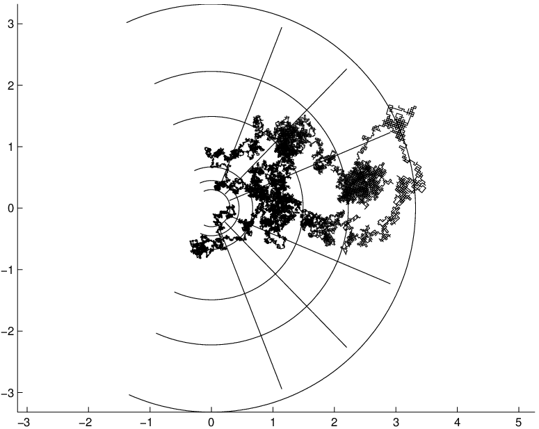
Actually, there exist only few known examples of probabilistic continuous models that are not directly related to Brownian motion. For instance, under mild regularity conditions, continuous finite-dimensional Markov processes are solutions of stochastic differential equations and therefore constructed using Brownian motions. If one looks for other types of continuous processes, one has therefore to give up the Markov property or the finite-dimensionality. In many complex systems that we see around us and for which probability theory seems a priori a well-suited tool (the shape of clouds, say), it is not possible to explain the phenomena via Brownian motions, and there is still a long way to go for probabilists to understand their macroscopic behaviour.

In the present lectures, we shall focus on random planar curves. In two dimensions, (random) curves appear naturally as boundaries of domains, interfaces between two phases, level lines of random surfaces etc. In all these cases, at least on microscopic level, the definition of the curve (say, as an interface) implies that it is a self-avoiding curve (or a simple closed loop). On the macroscopic scale, the continuous curves that we will be considering may have double-points (in the scaling limit, simple curves may converge to curves with multiple points), but self-crossings are forbidden. Of course, if $(\gamma_{t},t\in[0,T])$ is such a random curve, we see that in general, this condition implies a strong correlation between $\gamma[0,t]$ and $\gamma[t,T]$, so that the Markov property is lost (if we look at these curves as living in the two-dimensional space). As we shall see, there is a way to recover a Markov property for the random curves, using a coding of the curve in an infinite-dimensional space of conformal maps.

In order to guide the intuition about the family of random curves that we will be considering, it is helpful to have some discrete models in mind, for which one expects or can prove that they converge to this continuous object. We therefore start these lectures with the description of one measure on discrete random curves that turns out to converge in the scaling limit. This is actually the model that Oded Schramm considered when he invented these random curves that he called $SLE$ (for Stochastic Loewner Evolution, but we will replace this by Schramm-Loewner Evolution in these lectures).

For any ${\bf x}=(x_{0},\ldots,x_{m})$, we define the loop-erasure $L({\bf x})$ of ${\bf x}$ inductively as follows: $L_{0}=x_{0}$, and for all $j\geq 0$, we define inductively $n_{j}=\max\{n\leq m\ :\ x_{n}=L_{j}\}$ and

until $j=\sigma$ where $L_{\sigma}:=x_{m}$. In other words, we have erased the loops of ${\bf x}$ in chronological order. The number of steps $\sigma$ of $L$ is not fixed.

Suppose that $(X_{n},n\geq 0)$ is a recurrent Markov chain on a discrete state-space ${\cal S}$ started from $X_{0}=x$. Suppose that $A\subset{\cal S}$ is non-empty, and let $\tau_{A}$ denote the hitting time of $A$ by $X$. Let $p(x,y)$ denote the transition probabilities for the Markov chain $X$. We define the loop-erasure $L=L(X[0,\tau_{A}])=L^{A}$ of $X$ up to its hitting time of $A$. We call $\sigma$ the number of steps of $L^{A}$. For $y\in A$ such that with positive probability $L^{A}(\sigma)=X(\tau_{A})=y$, we call ${\cal L}(x,y;A)$ the law of $L^{A}$ conditioned on the event $\{L^{A}(\sigma)=y\}$. In other words, it is the law of the loop-erasure of the Markov chain $X$ conditioned to hit $A$ at $y$.

This Lemma shows that it is in fact fairly natural to index the loop-erased path backwards (define $\gamma_{j}=L^{A}_{\sigma-j}$, so that $\gamma$ starts on $A$ and goes back to $\gamma_{\sigma}=x$). Then, the time-reversal of loop-erased (conditioned and stopped) Markov chains have themselves a Markovian-type property.

Let us now come back to our two-dimensional setting: Suppose that $X$ is a simple random walk on the grid $\delta{\hbox{\m Z}}^{2}$ (we will then let the mesh $\delta$ of the lattice go to $0$) that is started from $0$. Let $D$ denote some simply connected domain $D$ with $0\in D$ and $D\not={\hbox{\m C}}$, and let $D_{\delta}=\delta{\hbox{\m Z}}^{2}\cap D$, $A=A_{\delta}=\delta Z^{2}\setminus D$. We are interested in the behaviour when $\delta\to 0$ of the law of $\gamma^{\delta}$ which is defined as before as the time-reversed loop-erasure of $X[0,\tau_{A}]$. We now think on a heuristic level: First, note that the law of $X_{\tau_{A}}$ converges to the harmonic measure on $\partial D$ from $0$, so that it is possible to study the behaviour of $\gamma^{\delta}$ conditional on the value of $\{\gamma^{\delta}=y_{0}^{\delta}\}$ where $y_{0}^{\delta}\to y\in\partial D$ as $\delta\to 0$. Second, one might argue that on the one hand, simple random walk converges to planar Brownian motion which is conformally invariant, and that on the other hand the chronological loop-erasing procedure is purely geometrical to conclude that when $\delta\to 0$, the law of $\gamma^{\delta}$ should converge to a conformal invariant curve that should be the loop-erasure of planar Brownian motion.

Unfortunately (or fortunately!), the geometry of planar Brownian curves is very complicated: It has points of any (even infinite) multiplicity (see e.g. LG), loops at any scale, so that there is no “first” loop to erase, and decisions about what small microscopic loops to erase first may propagate to the decisions about what macroscopic loops one should erase. In other words, there is no simple (even random) algorithm to loop-erase a Brownian path in chronological order. Yet, the previous heuristic strongly suggests the law of $\gamma^{\delta}$ should converge, and that the limiting law is invariant under conformal transformations: The scaling limit of LERW in $D$ should be (modulo time-change) identical to the conformal image of the scaling limit of LERW in $D^{\prime}$. Furthermore, Lemma 1 should still be valid in the scaling limit. We now show that the combinations of these two properties in fact greatly reduce the family of possible scaling limits for LERW.

We are therefore looking for the law of a random continuous curve $(\gamma_{t},t\geq 0)$ with no self-crossings in the unit disc 𝕌, with $\gamma_{0}=1$, $\lim_{t\to\infty}\gamma_{t}=0$ that could be the scaling limit of (time-reversed) loop-erased random walk on a grid approximation of 𝕌 (conditioned to exit 𝕌 near $1$). Define for each $t\geq 0$, the conformal map $f_{t}$ from ${\hbox{\m U}}\setminus\gamma[0,t]$ onto 𝕌 which is normalized by $f_{t}(0)=0$ and $f_{t}(\gamma_{t})=1$ (actually, if $\gamma$ would have double-points, the domain of definition would be the connected component of ${\hbox{\m U}}\setminus\gamma[0,t]$ that contains the origin, but let us a priori assume for convenience that $\gamma$ is a simple curve).

It is easy to check that $t\mapsto|f_{t}^{\prime}(0)|$ is an increasing continuous function that goes to $\infty$ as $t\to\infty$ (see for instance A2). Hence, it is possible to reparametrize $\gamma$ in such a way that

This is the natural parametrization in our context. Indeed, let us now study the conditional law of $\gamma[t,\infty)$ given $\gamma[0,t]$. Lemma 1 suggests that this law is the scaling limit of (time-reversed) LERW in the slit domain ${\hbox{\m U}}\setminus\gamma[0,t]$ conditioned to exit at $\gamma_{t}$, and conformal invariance then says that this is the same (modulo time-reparametrization) as the image under $z\mapsto f_{t}^{-1}(z)$ of an independent copy $\tilde{\gamma}$ of $\gamma$. Note that if one composes conformal maps that preserve the origin, then the derivative at the origin multiply: This shows that in fact, no time-change is necessary if we parametrize $\gamma$ (and $\tilde{\gamma}$) by (1.1), in order for the conditional law of $(\gamma_{t+s},s\geq 0)$ given $\gamma[0,t]$ to be identical to that of $(f_{t}^{-1}(\tilde{\gamma}_{s}),s\geq 0)$. In other words, for all fixed $t\geq 0$,

where $(\tilde{f}_{s},s\geq 0)$ is an independent copy of $(f_{s},s\geq 0)$. In particular, $f_{2t}=\tilde{f}_{t}\circ f_{t}$ in law. Repeating this procedure, we see that for all $t\geq 0$ and all integer $n\geq 1$, $f_{nt}$ is the iteration of $n$ independent copies of $f_{t}$, and that $f_{t}$ itself can be viewed as the iteration of $n$ independent copies of $f_{t/n}$. In other words, $(f_{t},t\geq 0)$ is an “infinitely divisible” process of conformal maps, and $f_{t}$ is obtained by iterating infinitely many independent conformal maps that are infinitesimally close to the identity.

Back in the 1920’s, Loewner observed that if $\gamma[0,\infty)$ is a simple continuous curve starting from $1$ in the unit disc, then it is naturally encoded via a continuous function $\zeta_{t}$ taking its values on the unit circle. Let us now describe briefly how it goes. Suppose, as in the previous section, that $\gamma(0)=1$, $\lim_{t\to\infty}\gamma_{t}=0$ and that $\gamma$ is parametrized in such a way that the modulus of the derivative at $0$ of the conformal map $f_{t}$ from $U_{t}:={\hbox{\m U}}\setminus\gamma[0,t]$ into 𝕌 that preserves the origin is $e^{t}$. Define $\zeta_{t}=(f_{t}^{\prime}(0)/|f_{t}^{\prime}(0)|)^{-1}$. In other words, if $g_{t}$ denotes the conformal map from $U_{t}$ onto 𝕌 such that $g_{t}(0)=0$ and $g_{t}^{\prime}(0)=e^{t}\in(0,\infty)$, then

and $g_{t}(z)=\zeta_{t}f_{t}(z)$. One can note (see e.g. A2; Dur) that for all $z\notin\gamma[0,t]$,

Hence, it is possible to recover $\gamma$ from $\zeta$ as follows: For all $z\in{\hbox{\m U}}$, define $g_{t}(z)$ as the unique solution to (1.2) starting from $z$. In case $g_{t}(z)=\zeta_{t}$ for some time $t$, then define $\gamma_{t}=g_{t}^{-1}(\zeta_{t})$ (we know already a priori that since $\gamma$ is a simple curve, the map $g_{t}^{-1}$ extends continuously to the boundary). Note that if $g_{t}(z)=\zeta_{t}$, then $g_{s}(z)$ is not well-defined for $s\geq t$.

Hence, in order to define the random curve $\gamma$ that should be the scaling limit of loop-erased random walks, it suffices to define the random function $\zeta_{t}=\exp(iW_{t})$, where $(W_{t},t\geq 0)$ is real-valued. Our previous considerations suggest that the following conditions should be satisfied:

• •

  The process $W$ is almost surely continuous.

• •

  The process $W$ has stationary increments (this is because $g_{t}$ is obtained by iterations of identically distributed conformal maps)

• •

  The laws of the processes $W$ and $-W$ are identical (this is because the law of $L$ and the law of the complex conjugate $\overline{L}$ are identical).

The theory of Markov processes tells us that the only possible choices are: $W_{t}=\beta_{\kappa t}$ where $\beta$ is standard Brownian motion and $\kappa\geq 0$ a fixed constant. In order to simplify some future notations, we will usually write

where $(B_{t},t\geq 0)$ is standard (one-dimensional) Brownian motion.

In summary, we have just seen that on a heuristic level, if the scaling limit of loop-erased random walk exists and is conformally invariant, then the scaling limit in the unit disk should be described as follows: For some fixed constant $\kappa=\kappa_{LERW}$, define $\zeta_{t}=\exp(i\sqrt{\kappa}B_{t}),t\geq 0$, solve for each $z\in{\hbox{\m U}}$, the equation (1.2) with $g_{0}(z)=z$. This defines a conformal map $g_{t}$ from the subset $U_{t}$ of the unit disk onto 𝕌. Then, one can construct $\gamma$ because

and

As we shall see later on in the lectures, this heuristic arguments can be made rigorous, and it will turn out that $\kappa_{LERW}=2$.

In the context of LERW, the random curve joins a point in the inside of the domain to a point on the boundary of the domain. In statistical physics models, one is often interested in “interfaces”. Some of these interfaces appear to be random curves from one point on the boundary to another point on the boundary. A natural setup is to study curves from $0$ to infinity in the upper half-plane ${\hbox{\m H}}:=\{x+iy\ :\ y>0\}$. Then, we look for random non-self-crossing curves $\gamma$ such that the law of $\gamma[t,\infty)$ given $\gamma[0,t]$ has the same law than the conformal image of an independent copy $\tilde{\gamma}$ of $\gamma$ under a conformal map from ℍ onto ${\hbox{\m H}}\setminus\gamma[0,t]$ that maps $\infty$ onto itself and $0$ onto $\gamma_{t}$.

We now very briefly describe an important discrete model for which it has now also been proved that it behaves in a conformally invariant way in the scaling limit (more details on the model and its conformal covariance will be given in Chapter 10): Critical site percolation on the triangular lattice. Actually, it is more convenient to describe this in terms of cell-colouring of the honeycombe lattice. Suppose that a simply connected domain $D$ is fixed, as well as two distinct points $a$ and $b$ on $\partial D$. Let $D_{\delta}$ denote a suitably chosen approximation of $D$ by a simply connected union of hexagonal cells of size $\delta$. Let $a_{\delta}$ (resp. $b_{\delta}$) denote a vertex of the honeycombe lattice on $\partial D_{\delta}$ that is close to $a$ (resp. to $b$). Then, the cells on $\partial D_{\delta}$ can be divided into two “arcs” $B_{\delta}$ and $W_{\delta}$ in such a way that $a_{\delta}$, $B_{\delta}$, $b_{\delta}$ and $W_{\delta}$ are oriented clockwise “around” $D_{\delta}$. Decide that all hexagons in $B_{\delta}$ are colored in black and that all hexagons in $W_{\delta}$ are colored in white. On the other hand, all other cells in $D_{\delta}$ are chosen to be black or white with probability $1/2$ independently of each other. Consider now the (random) path $\gamma_{\delta}$ from $a_{\delta}$ to $b_{\delta}$ that separates the cluster of black hexagons containing $B_{\delta}$ from the cluster of white hexagons containing $W_{\delta}$.

For deep reasons that will be discussed later in these lectures, it will turn out that when $\delta\to 0$, the law of $\gamma_{\delta}$ converges towards that of a random curve $\gamma$ from $a$ to $b$ in $D$, and that the law of that curve is conformally invariant: The law of $\Phi(\gamma)$ when $\Phi$ is a conformal map from $D$ onto $\Phi(D)$ is that of the corresponding path (i.e. of the scaling limit of percolation cluster interfaces) from $\Phi(a)$ to $\Phi(b)$ in $\Phi(D)$.

Again, on the discrete level, it is easy to see that $\gamma_{\delta}$ has the same type of Markovian property that LERW. More precisely, conditioning on the first steps of $\gamma$ is equivalent to condition the percolation process to have black hexagons on the left-boundary of these steps and white hexagons on the right side. Hence, the conditional law of the remaining steps is that of the percolation interface in the new domain obtained by slitting $D_{\delta}$ along the first steps of $\gamma_{\delta}$. Figure 1.4 shows the beginning of the interface $\gamma_{\delta}$ in the case where $D$ is the upper half-plane.

Another equivalent way to define the interface $\gamma_{\delta}$ goes as follows: It is a myopic self-avoiding walk. At each step $\gamma_{\delta}$ looks at its three neighbours (on the honeycomb lattice) and chooses at random one of the sites that it has not visited yet (there are one or two such sites since one site is anyway forbidden because it was the previous location of the walk).

This discrete walk in the upper half-plane is a very special discrete model that will turn out to converge to an SLE. The corresponding value of $\kappa$ is $6$. Here, the starting point $a=0$ and the end-point $b=\infty$ are both on the boundary of the domain, so that the previous definition of radial SLE is not well-suited anymore.

The natural time-parametrization in the previous setup goes as follows: Let $g_{t}$ denote the conformal map from ${\hbox{\m H}}\setminus\gamma[0,t]$ onto ℍ that is normalized at infinity in the sense that when $z\to\infty$,

It is easy to see that $a_{t}$ is positive, increasing and that it is natural to parametrize $g_{t}$ in such a way that $a_{t}$ is a multiple of $t$ (since the $a_{t}$ terms add up when one composes two such conformal maps). It is natural to choose $a_{t}=2t$ (this is consistent with the chosen parametrization in the radial case). Then, define $w_{t}=g_{t}(\gamma_{t})$, and observe that

Hence, just as in the radial case, we observe that it is possible to recover $\gamma$ using $w$, and that the only choice for $w$ that is consistent with the “Markovian property” is to take $w_{t}=\sqrt{\kappa}B_{t}$, where $B$ is ordinary one-dimensional Brownian motion.

Hence, one is lead to the following definition: Let $w_{t}=\sqrt{\kappa}B_{t}$, and define for all $z\in\overline{{\hbox{\m H}}}$, the solution $g_{t}(z)$ of (1.3) up to the (possibly infinite) time $T(z)$ at which $g_{t}(z)$ hits $w_{t}$. Then, define

and

Then, $g_{t}$ is the normalized conformal map from $H_{t}$ onto ℍ. We call $(K_{t},t\geq 0)$ the chordal $SLE_{\kappa}$ in the upper half-plane.

It turns out that radial and chordal SLE’s are rather closely related: Consider for instance, the conformal image of radial $SLE_{\kappa}$ under the map that maps 𝕌 onto ℍ, $1$ to $0$ and $0$ to $i$. Consider both this process and chordal $SLE_{\kappa}$ up to their first hitting of the circle of radius $1/2$ around zero say. Then, the laws of these two processes are absolutely continuous with respect to each other LSW2. This justifies a posteriori the choice of time-parametrization in the chordal case.

We have seen that if one considers a discrete model of random curves (or interfaces) that combine the two important features:

• •

  The Markovian type property in the discrete setting,

• •

  Conformal invariance in the limit when the mesh of the lattice goes to zero,

then the good way to construct the possible candidates for the scaling limit of these curves is to encode them via the corresponding conformal mappings. Then, these (random) conformal mappings are themselves obtained by iterations of identically distributed random conformal maps. Loewner’s theory shows that such families of conformal maps are themselves encoded by a one-dimensional function. If one knows this one-dimensional function, one can recover the family of conformal maps, and therefore also the two-dimensional curve. The one-dimensional random function that generates the scaling limits of the discrete models must necessarily be a one-dimensional Brownian motion. The corresponding random two-dimensional curves are SLE processes.

We study increasing “continuously growing” compact subsets $(K_{t},t\geq 0)$ of the upper half-plane. It will turn out to be important to choose the good time-parametrization. We want to find the natural way to measure the size $a(K)$ of a compact set $K$ and we will then choose the time-parametrization in such a way that $a(K_{t})=t$. We will use the following definition throughout the paper.

Riemann’s mapping theorem asserts that there exist conformal maps $\Phi$ from $H$ onto ℍ with $\Phi(\infty)=\infty$. Actually, if $\Phi$ is such a map, the family of maps $b\Phi+b^{\prime}$ for real $b^{\prime}$ and positive $b$ is exactly the family of conformal maps from $H$ onto ℍ that fix infinity.

Note that since $K$ is compact, the mapping $\Psi:z\mapsto 1/\Phi(1/z)$ is well-defined on a neighbourhood of $0$ in ℍ. It is possible to extend this map $\Psi$ to a whole neighbourhood of $0$ in the plane by reflection along the real axis (this is usually called Schwarz reflection) and to check that this extension is analytic. This implies that $\Phi$ can be expanded near infinity: There exist $b_{1},b_{0},b_{-1},\ldots$, such that

when $z\to\infty$ in ℍ. Furthermore, since $\Phi$ preserves the real axis near infinity, all coefficients $b_{j}$ are real.

Hence, for each $K$, there exists a unique conformal map $\Phi=\Phi_{K}$ from $H={\hbox{\m H}}\setminus K$ onto ℍ such that:

This is sometimes called the hydrodynamical normalization. In particular, there exists a real $a=a(K)$ such that

This number $a(K)$ is a way to measure the size of $K$. In a way, it tells “how big $K$ is in ℍ, seen from infinity”. It may a priori not be clear that $a$ is a non-negative increasing function of the set $K$. There is a simple probabilistic interpretation of $a(K)$ that immediately implies these facts: Suppose that $Z=X+iY$ is a complex Brownian motion started from $Z_{0}=iy$ (for some large $y$, so that $Z_{0}\notin K$) and stopped at its first exit time $\tau$ of $H$. The expansion $\Phi(z)=z+o(1)$ near infinity shows that $\Im(\Phi(z)-z)$ is a bounded harmonic function in $H$. The martingale stopping theorem therefore shows that

But $\Phi(Z_{\tau})$ is real because of the definition of $\tau$. Therefore

In particular, $a\geq 0$.

One can also view $a$ as a function of the normalized conformal map $\Phi_{K}$ instead of $K$. The chain rule for Taylor expansions then immediately shows that

for any two normalized maps $\Phi^{1}$ and $\Phi^{2}$. In particular, this readily implies that $a(K)\leq a(K^{\prime})$ if $K\subset K^{\prime}$ (because there exists a normalized conformal map from ${\hbox{\m H}}\setminus\Phi_{K}(K^{\prime}\setminus K)$ onto ℍ).

Let us now observe two simple facts:

• •

  If $\lambda>0$, then $a(\lambda K)=\lambda^{2}a(K)$. This is simply due to the fact that

  $$\Phi(z/\lambda)=\frac{z}{\lambda}+\frac{2a(K)\lambda}{z}+o(\lambda/z)$$

  so that

  $$\Phi_{\lambda K}(z)=\lambda\Phi_{K}(z/\lambda)=z+\frac{2a(K)\lambda^{2}}{z}+o\lambda(\lambda/z)$$

  (2.1)

  when $z\to\infty$.

• •

  When $K$ is the vertical slit $[0,iy]$, then

  $$\Phi_{K}(z)=\sqrt{z^{2}+y^{2}}.$$

  In particular, we see that $a([0,iy])=y^{2}/4$. Note that if $y$ is very small, the actual diameter of the vertical slit $[0,iy]$ is much larger than $a([0,iy])$.

Equation (2.1) shows that for all $K$ such that $a(K)=1$, one has $a(\sqrt{\lambda}K)=\lambda$ and

Actually, it is not very difficult to prove that for all given $r$, there exists $C>0$ such that this convergence takes place uniformly over all $K$ of radius smaller than $r$ and $|z|>Cr$. See Lemma 2.7 in LSW1.

Suppose that a continuous real function $w_{t}$ with $w_{0}=0$ is given. For each $z\in\overline{{\hbox{\m H}}}$, define the function $g_{t}(z)$ as the solution to the ODE

with $g_{0}(z)=z$. This is well-defined as long as $g_{t}(z)-w_{t}$ does not hit $0$, i.e., for all $t<T(z)$, where

We define

Note for instance that if $w_{t}=0$ for all $t$, then

and $K_{t}=[0,2i\sqrt{t}]$.

It is very easy to check that $g_{t}$ is a bijection from $H_{t}$ onto ℍ (in order to see that it is surjective, one can just look at the ODE “backwards in time” to find which point $z$ is such that $g_{t}(z)=y$). Moreover $K_{t}$ is bounded (because $w$ is continuous and bounded on $[0,t]$) and $H_{t}$ has a unique connected component (because $g_{t}^{-1}$ is continuous). Standard arguments from the theory of ordinary differential equations can be applied to check that $g_{t}$ is analytic and that one can formally differentiate the ODE with respect to $z$, so that

So, $g_{t}$ is a conformal map from $H_{t}$ onto ℍ.

Note also that $|\partial_{t}g_{t}(z)|$ is uniformly bounded when $z$ is large and $t$ belongs to a given finite interval $[0,t_{0}]$. Hence, it follows that $g_{t}(z)=z+O(1)$ near infinity and uniformly over $t\in[0,t_{0}]$. Hence (using the ODE yet again), $\partial_{t}g_{t}(z)=2/z+o(1/z)$ uniformly over $t\in[0,t_{0}]$ so that finally, for each $t$,

when $z\to\infty$. In other words, $a(K_{t})=t$. The family $(K_{t},t\geq 0)$ is called the Loewner chain associated to the driving function $(w_{t},t\geq 0)$.

Loewner’s original motivation was to control the behaviour of the coefficients of the Taylor expansion of conformal maps and for this goal, it is sufficient to consider smooth slit domains (see e.g., A2; Dur). For this reason, the following question was only addressed later (see Ku): If the continuous function $(w_{t},t\geq 0)$ is given, what can be said about the family of compact sets $(K_{t},t\geq 0)$?

In the introduction, we started with a continuous curve $\gamma$, then using $\gamma$, we defined $H_{t}$, the conformal maps $g_{t}$, the function $w_{t}$ and argued that one could recover $\gamma$ from $w_{t}$, using the fact that we a priori knew that $g_{t}^{-1}$ extends continuously to $w_{t}\in\partial{\hbox{\m H}}$ and that $g_{t}^{-1}(w_{t})$ was well-defined (and equal to $\gamma_{t}$) because $\gamma$ is a continuous curve. But if one starts with a general continuous function $w_{t}$, then it can in fact happen that $g_{t}^{-1}$ does not extend continuously to $w_{t}$.

Before making general considerations, let us exhibit a simple example to show that $(K_{t},t\geq 0)$ does not need to be a simple curve. For $\theta\in[0,\pi)$, let $\eta(\theta)=\exp(i\theta)-1$. Define $t(\theta)=a(\eta[0,\theta])$ the “size” of the arc $\eta[0,\theta]$. Finally, define the reparametrization $\gamma$ of $\eta$ in such a way that $a(\gamma[0,t])=t$. $\gamma$ is defined for all $t<T:=\lim_{\theta\to\pi-}a(\eta[0,\theta])$. It is simple to see that there exists a continuous function $(w_{t},t<T)$ such that the normalized conformal maps $g_{t}$ from ${\hbox{\m H}}\setminus\gamma[0,t]$ onto ℍ satisfy the equation (2.3). Furthermore, when $t\to T-$, $w_{t}$ converges to a finite limit $w_{T}$. At time $T$, the curve $\gamma[0,T]$ disconnects the inside of the semi-circle from the outside. Just before $T$, because $g_{t}$ is normalized “from infinity”, the inside of the semi-circle is mapped onto a small region which is very close to $w_{t}=g_{t}(\gamma_{t})$. When $t\to T-$, all points inside the semi-circle are hitting $w_{T}$. In other words, $K_{T}$ is the whole semi-disc, $H_{T}$ is the complement of the semi-disc, and $g_{T}$ is the normalized map from the simply connected domain $H_{T}$ onto ℍ.

Let us now give a couple of general definitions:

• •

  We say that $(K_{t},t\geq 0)$ is a simple curve if there exists a simple continuous curve $\gamma$ such that $K_{t}=\gamma[0,t]$.

• •

  We say that $(K_{t},t\geq 0)$ is generated by a curve if there exists a continuous curve $\gamma$ with no self-crossings, such that for all $t\geq 0$, $H_{t}={\hbox{\m H}}\setminus K_{t}$ is the unbounded connected component of ${\hbox{\m H}}\setminus\gamma[0,t]$. In other words, $K_{t}$ is the union of $\gamma$ and of the inside of the loops that $\gamma$ creates.

• •

  We say that $(K_{t},t\geq 0)$ is pathological if it is not generated by a curve.

In each of these three cases, one can find (deterministic) continuous functions $w_{t}$ such that the family $(K_{t},t\geq 0)$ that it constructs falls into this category: For the first case, consider for instance $w_{t}=0$ as before, for the second case, one can use the example with the semi-circle. For the more intricate third case, let us mention the following example (due to Don Marshal and Steffen Rohde, see MR): Let $\gamma$ denote a simple curve in ℍ started from $\gamma_{0}=0$ that spirals clockwise around the segment $[i,2i]$ an infinite number of times, and then unwinds itself. Then at the “time” at which it winds around the segment an infinite number of times, $\gamma$ is not continuous i.e. $K_{t}\setminus K_{t-}$ is the whole segment. However, this Loewner chain corresponds to a continuous function $w_{t}$. Such pathologies could arise at any scale.

We now characterize the families $(K_{t},t\geq 0)$ of compact sets that are Loewner chains:

Suppose now that $K_{t}$ is the Loewner chain

for some $c=c(\theta)\exp(i\theta)\in{\hbox{\m H}}$. Here, $\theta\not=0$ is given, and then the positive real $c(\theta)$ is chosen in such a way that $a(K_{1})=1$. Scaling immediately shows that $a(K_{t})=t$ for all $t>0$, so that there exists therefore a continuous driving function $w$ that generates these slits. Again, scaling (because $K_{\lambda t}=\sqrt{\lambda}K_{t}$) shows that necessarily, this function $w$ must be of the type

for some real constant $c_{1}=c_{1}(\theta)$. Let $g_{t}^{\theta}$ denote the corresponding family of conformal maps.

Let us now choose a new driving function $w$ as follows: $w_{t}=0$ when $t<1$ and for $t\geq 1$:

When $t<1$, then $K_{t}$ is just the straight slit. In particular, $g_{1}(z)=\sqrt{z^{2}+4}$. When $t>1$, then $K_{t}$ is obtained by mapping the angled slit $K_{t-1}^{\theta}$ back by $g_{1}^{-1}$. In particular, we see that the curve $\gamma$ generated by this function $w$ is not differentiable at $t=1$. This is one simple hint to the fact that Hölder-$1/2$ regularity may be critical (note that at $t=1$, $w$ is just Hölder $1/2$).

The general relation between smoothness of the driving function and regularity of the slit has also recently been investigated (in the deterministic setting) by Marshall-Rohde MR. In this paper, it is shown that Hölder-$1/2$ is in a sense a “critical regularity” for the driving function $w_{t}$: Loosely speaking (their results are more precise than that), if $w$ is better than Hölder-$1/2$, then it defines a “smooth” (in some appropriate sense) slit, but nasty “pathological” phenomena can occur for Hölder-$1/2$ driving functions. See MR and the references therein.

For general background on complex analysis, Riemann’s mapping theorem, there are plenty of good references, see for instance A1; Ru. Loewner introduced his equation (in the radial setting) in 1923 Lo. For general information about Loewner’s equation, and in particular how Loewner used it to prove that $|a_{3}|\leq 3$ for univalent functions $z+\sum_{n\geq 2}a_{n}z^{n}$ on 𝕌 as well as other applications, see for instance A2; Dur. For how it is used in de Branges’ proof of the Bieberbach conjecture, a good self-contained reference is Hayman’s book Hay. For basics on hypergeometric functions, see e.g., Le.

Proposition 2.2.1 is derived in LSW1, see also Po. Carleson and Makarov CM1; CM2 have used Loewner’s (radial) equation in the context of Diffusion Limited Aggregation.

Chordal $SLE_{\kappa}$ is the Loewner chain $(K_{t},t\geq 0)$ that is obtained when the driving function

is $\sqrt{\kappa}$ times a standard real-valued Brownian motion $(B_{t},t\geq 0)$ with $B_{0}=0$. Let us now list a couple of consequences of the simple properties of Brownian motion:

• •

  Brownian motion is a strong Markov process with independent increments. This implies that for any stopping time $T$ (with respect to the natural filtration $({\cal F}_{t},t\geq 0)$ of $B$), the process

  $$(g_{T+t}(K_{T+t}\setminus K_{T})-W_{T},t\geq 0)$$

  is independent of ${\cal F}_{T}$ and that its law is identical to that of $(K_{t},t\geq 0)$. Note that one has to shift by $W_{T}$ in order to obtain a process starting at the origin.

• •

  Brownian motion is scale-invariant: For each $\lambda>0$, the process $W_{t}^{\lambda}:=W_{\lambda t}/\sqrt{\lambda},t\geq 0$ has the same law than $W$. But

  $$\partial_{t}(g_{\lambda t}(\sqrt{\lambda}z))=\frac{2\lambda}{g_{t}(\sqrt{\lambda}z)-W_{\lambda t}}.$$

  In particular, if

  $$g_{t}^{\lambda}(z):=g_{\lambda t}(z\sqrt{\lambda})/\sqrt{\lambda},$$

  then

  $$\partial_{t}g_{t}^{\lambda}(z)=\frac{2}{g_{t}^{\lambda}(z)-W_{t}^{\lambda}}$$

  and $g_{0}^{\lambda}(z)=z$. In other words, $(K_{\lambda t},t\geq 0)$ and $(\sqrt{\lambda}K_{t},t\geq 0)$ have the same law: Chordal $SLE_{\kappa}$ is scale-invariant.

• •

  Brownian motion is symmetric ($W$ and $-W$ have the same law). Hence, the law of $(K_{t},t\geq 0)$ is symmetric with respect to the imaginary axis.

It is actually possible to prove the following result:

This result is due to Rohde-Schramm RS (see LSWlesl for the critical case $\kappa=8$). It is not an easy result, especially for the values $\kappa>4$. Actually, while this fact is important and useful in order to understand heuristically the behaviour and the properties of $SLE_{\kappa}$, it turns out that one can derive many of them without knowing that the $SLE_{\kappa}$ is generated by a continuous curve. We therefore omit the proof in these lectures, and we will call $(K_{t},t\geq 0)$ the SLE. In some cases that we will focus on ($\kappa=2,8/3,6,8$), the fact that $SLE_{\kappa}$ is a.s. generated by a curve will actually follow from other considerations.

References

- (1) L.V. Ahlfors, Complex analysis, 3rd Ed., McGraw-Hill, New-York, 1978.
- (2) L.V. Ahlfors, Conformal Invariants, Topics in Geometric Function Theory, McGraw-Hill, New-York, 1973.
- (3) M. Aizenman (1996), The geometry of critical percolation and conformal invariance, Statphys19 (Xiamen, 1995), 104-120.
- (4) M. Aizenman (1998), Scaling limit for the incipient spanning clusters, in Mathematics of multiscale materials, IMA Vol. Math. Appl. 99, Springer, New York, 1-24.
- (5) M. Aizenman, A. Burchard (1999), Hölder regularity and dimension bounds for random curves, Duke Math. J. 99, 419–453.
- (6) M. Aizenman, A. Burchard, C.M. Newman, D.B. Wilson (1999), Scaling limits for minimal and random spanning trees in two dimensions. Random Structures Algorithms 15, 319-367.
- (7) M. Aizenman, B. Duplantier, A. Aharony (1999), Path crossing exponents and the external perimeter in 2D percolation. Phys. Rev. Let. 83, 1359-1362.
- (8) O. Angel (2002), Growth and Percolation on the Uniform Infinite Planar Triangulation, preprint.
- (9) O. Angel, O. Schramm (2002), Uniform Infinite Planar Triangulations, preprint.
- (10) M. Bauer, D. Bernard (2002), growth processes and conformal field theories Phys. Lett. B543, 135-138.
- (11) M. Bauer, D. Bernard (2002), Conformal Field Theories of Stochastic Loewner Evolutions, preprint.
- (12) M. Bauer, D. Bernard (2003), SLE martingales and the Virasoro algebra, preprint.
- (13) V. Beffara (2001), On some conformally invariant subsets of the planar Brownian curve, Ann. Inst. Henri Poincaré, to appear
- (14) V. Beffara (2002), Hausdorff dimensions for , preprint.
- (15) V. Beffara (2002), The dimension of the SLE curves, preprint.
- (16) V. Beffara, in preparation
- (17) A.A. Belavin, A.M. Polyakov, A.B. Zamolodchikov (1984), Infinite conformal symmetry of critical fluctuations in two dimensions, J. Statist. Phys. 34, 763–774.
- (18) A.A. Belavin, A.M. Polyakov, A.B. Zamolodchikov (1984), Infinite conformal symmetry in two-dimensional quantum field theory. Nuclear Phys. B 241, 333–380.
- (19) I. Benjamini, G. Kalai, O. Schramm (1999), Noise sensitivity of boolean functions and applications to percolation, Publ. Sci. IHES 90, 5-43.
- (20) I. Benjamini, R. Lyons, Y. Peres, O. Schramm (2001), Uniform spanning forests. Ann. Probab. 29, 1-65.
- (21) I. Benjamini, O. Schramm (1998), Conformal invariance of Voronoi percolation, Comm. Math. Phys. 197, 75-107.
- (22) J. van den Berg, A. Ermakov (1996), A new lower bound for the critical probability of site percolation on the square lattice, Random Structures Algorithms 8,199-212.
- (23) R. van den Berg, A. Jarai (2001), The lowest crossing in 2D critical percolation, preprint
- (24) C.J. Bishop, P.W. Jones, R. Pemantle, Y. Peres (1997), The dimension of the Brownian frontier is greater than , J. Funct. Anal. 143, 309–336.
- (25) M. Bousquet-Mélou, G. Schaeffer (2002), The degree distribution in bipartite planar maps: applications to the Ising model, preprint.
- (26) J. Bouttier, B. Eynard, Ph. Di Francesco (2002), Combinatorics of Hard Particles on Planar Graphs, preprint.
- (27) K. Burdzy, G.F. Lawler (1990), Non-intersection exponents for random walk and Brownian motion. I: Existence and an invariance principle, Probab. Theor. Rel. Fields 84, 393–410.
- (28) K. Burdzy, G.F. Lawler (1990), Non-intersection exponents for random walk and Brownian motion. II: Estimates and applications to a random fractal, Ann. Prob. 18, 981-1009.
- (29) R. Burton, R. Pemantle (1993), Local characteristics, entropy and limit theorems for spanning trees and domino tilings via transfer-impedances, Ann. Probab. 21, 1329–1371.
- (30) J.L. Cardy (1984), Conformal invariance and surface critical behavior, Nucl. Phys. B 240 (FS12), 514–532.
- (31) J.L. Cardy (1992), Critical percolation in finite geometries, J. Phys. A, 25 L201–L206.
- (32) J.L. Cardy, Scaling and renormalization in statistical physics, Cambridge Lecture Notes in Physics 5, Cambridge University Press, 1996.
- (33) J.L. Cardy (1998), The number of incipient spanning clusters in two-dimensional percolation, J. Phys. A 31, L105.
- (34) J.L. Cardy (2001), Lectures on Conformal Invariance and Percolation, Lectures delivered at Chuo University, Tokyo, preprint.
- (35) L. Carleson, N.G. Makarov (2001), Aggregation in the plane and Loewner’s equation, Comm. Math. Phys. 216, 583-607.
- (36) L. Carleson, N.G. Makarov (2002), Laplacian path models, preprint
- (37) M. Cranston, T. Mountford (1991), An extension of a result by Burdzy and Lawler, Probab. Th. Relat. Fields 89, 487–502.
- (38) M.P.M. Den Nijs (1979), A relation between the temperature exponents of the eight-vertex and the -state Potts model, J. Phys. A 12, 1857-1868.
- (39) J. Dubédat (2003), SLE and triangles, El. Comm. Probab. 8, 28-42.
- (40) J. Dubédat (2003), martingales and duality, preprint.
- (41) J. Dubédat (2003), Reflected planar Brownian motion, intertwining relations and crossing probabilities, preprint.
- (42) J. Dubédat (2003), preprint.
- (43) B. Duplantier (1992), Loop-erased self-avoiding walks in two dimensions: exact critical exponents and winding numbers, Physica A 191, 516–522.
- (44) B. Duplantier (1998), Random walks and quantum gravity in two dimensions, Phys. Rev. Lett. 81, 5489–5492.
- (45) B. Duplantier (1999), Harmonic measure exponents for two-dimensional percolation, Phys. Rev. Lett. 82, 3940-3943.
- (46) B. Duplantier (2000), Conformally invariant fractals and potential theory, Phys. Rev. Lett. 84, 1363-1367.
- (47) B. Duplantier (2003), Conformal Fractal Geometry and Boundary Quantum Gravity, preprint
- (48) B. Duplantier, K.-H. Kwon (1988), Conformal invariance and intersection of random walks, Phys. Rev. Let. 61, 2514–2517.
- (49) P.L. Duren, Univalent functions, Springer, 1983.
- (50) S. Fomin (2001), Loop-erased walks and total positivity, Trans. Amer. Math. Soc. 353, 3563–3583.
- (51) R. Friedrich, J. Kalkkinen (2003), preprint.
- (52) R. Friedrich, W. Werner (2002), Conformal fields, restriction properties, degenerate representations and SLE, C.R. Ac. Sci. Paris Ser. I Math 335, 947-952.
- (53) R. Friedrich, W. Werner (2003), Conformal restriction, highest-weight representations and SLE, preprint.
- (54) T. Grossman, A. Aharony (1987), Accessible external perimeters of percolation clusters, J.Physics A 20, L1193-L1201
- (55) G.R. Grimmett, Percolation, Springer, New-York, 1989.
- (56) G.R. Grimmett (1997), Percolation and disordered systems, Ecole d’été de Probabilités de St-Flour XXVI, L.N. Math. 1665, 153-300
- (57) O. Häggström (1995), Random-cluster Measures and Uniform Spanning Trees, Stoch. Proc. Appl. 59, 267-275
- (58) W.K. Hayman, Multivalent functions, CUP, 1994 (second edition).
- (59) N. Ikeda and S. Watanabe, Stochastic Differential Equations and Diffusion Processes, Second edition, North-Holland, 1989.
- (60) T. Kennedy (2002), A faster implementation of the pivot algorithm for self-avoiding walks, J. Stat. Phys. 106, 407-429.
- (61) T. Kennedy (2002), Monte Carlo Tests of Stochastic Loewner Evolution Predictions for the 2D Self-Avoiding Walk, Phys. Rev. Lett. 88, 130601.
- (62) R. Kenyon (1997), Local statistics of lattice dimers, Ann. Inst. Henri Poincaré 33, 591-618.
- (63) R. Kenyon (1999), Dimères et arbres couvrants, in Mathématique et Physique, SMF Journ. Annu., 1-14.
- (64) R. Kenyon (2000), Conformal invariance of domino tiling, Ann. Probab. 28, 759-785.
- (65) R. Kenyon (2000), The asymptotic determinant of the discrete Laplacian, Acta Math. 185, 239-286.
- (66) R. Kenyon (2000), Long-range properties of spanning trees in , J. Math. Phys. 41 1338–1363.
- (67) H. Kesten, Percolation theory for mathematicians, Birhäuser, Boston, 1982.
- (68) H. Kesten (1987), Scaling relations for 2D-percolation, Comm. Math. Phys. 109, 109-156.
- (69) H. Kesten, V. Sidoravicius, Yu. Zhang (2001), Percolation of Arbitrary words on the Close-Packed Graph of , Electr. J. Prob. 6, paper no. 4.
- (70) V.G. Knizhnik, A.M. Polyakov, A.B. Zamolodchikov (1988), Fractal structure of 2-D quantum gravity, Mod. Phys. Lett. A3, 819.
- (71) G. Kozma (2002), Scaling limit of loop erased random walk - a naive approach, preprint.
- (72) P.P. Kufarev (1947), A remark on integrals of the Loewner equation, Dokl. Akad. Nauk SSSR 57, 655-656.
- (73) R. Langlands, Y. Pouillot, Y. Saint-Aubin (1994), Conformal invariance in two-dimensional percolation, Bull. A.M.S. 30, 1–61.
- (74) G.F. Lawler (1980), A self-avoiding random walk, Duke Math. J. 47, 655-694.
- (75) G.F. Lawler, Intersections of Random Walks, Birkhäuser, Boston, 1991.
- (76) G.F. Lawler (1995), Nonintersecting planar Brownian motions, Mathematical Physics Electronic Journal 1, paper no.1.
- (77) G.F. Lawler (1996), Hausdorff dimension of cut points for Brownian motion, Electron. J. Probab. 1, paper no.2.
- (78) G.F. Lawler (1996), The dimension of the frontier of planar Brownian motion, Electron. Comm. Prob. 1, paper no.5.
- (79) G.F. Lawler (1997), The frontier of a Brownian path is multifractal, preprint.
- (80) G.F. Lawler (1998), Strict concavity of the intersection exponent for Brownian motion in two and three dimensions, Mathematical Physics Electronic Journal 5, paper no. 5.
- (81) G.F. Lawler (1999), Loop-erased random walk, in Perplexing problems in Probability, Prog. Prob. 44, Birkhäuser, 197-217.
- (82) G.F. Lawler (1999), Geometric and fractal properties of Brownian motion and random walk paths in two and three dimensions, Bolyai Mathematical Society Studies, 9, 219-258.
- (83) G.F. Lawler (2001), An introduction to the stochastic Loewner evolution, preprint.
- (84) G.F. Lawler, E.E. Puckette (1997), The disconnection exponent for simple random walk, Israel J. Math. 99, 109-122.
- (85) G.F. Lawler, E.E. Puckette (2000), The intersection exponent for simple random walk, Combin. Probab. Comput. 9, 441-464.
- (86) G.F. Lawler, O. Schramm, W. Werner (2001), Values of Brownian intersection exponents I: Half-plane exponents, Acta Mathematica 187, 237-273.
- (87) G.F. Lawler, O. Schramm, W. Werner (2001), Values of Brownian intersection exponents II: Plane exponents, Acta Mathematica 187, 275-308.
- (88) G.F. Lawler, O. Schramm, W. Werner (2002), Values of Brownian intersection exponents III: Two sided exponents, Ann. Inst. Henri Poincaré 38, 109-123.
- (89) G.F. Lawler, O. Schramm, W. Werner (2002), Analyticity of planar Brownian intersection exponents, Acta Mathematica 189, to appear.
- (90) G.F. Lawler, O. Schramm, W. Werner (2001), The dimension of the planar Brownian frontier is , Math. Res. Lett. 8, 401-411.
- (91) G.F. Lawler, O. Schramm, W. Werner (2001), Sharp estimates for Brownian non-intersection probabilities, in: In and Out of Equilbrium, V. Sidoravicius Ed., Prog. Probab. 51, Birkhäuser, 113-131.
- (92) G.F. Lawler, O. Schramm, W. Werner (2002), One-arm exponent for critical 2D percolation, Electronic J. Probab. 7, paper no.2.
- (93) G.F. Lawler, O. Schramm, W. Werner (2001), Conformal invariance of planar loop-erased random walks and uniform spanning trees, preprint.
- (94) G.F. Lawler, O. Schramm, W. Werner (2002), On the scaling limit of planar self-avoiding walks, preprint.
- (95) G.F. Lawler, O. Schramm, W. Werner (2002), Conformal restriction properties. The chordal case, preprint.
- (96) G.F. Lawler, W. Werner (1999), Intersection exponents for planar Brownian motion, Ann. Probab. 27, 1601-1642.
- (97) G.F. Lawler, W. Werner (2000), Universality for conformally invariant intersection exponents, J. Europ. Math. Soc. 2, 291-328.
- (98) G.F. Lawler, W. Werner (2003), The Brownian loop-soup, preprint.
- (99) N.N. Lebedev, Special Functions and their Applications, transl. from russian, Dover, 1972.
- (100) J.F. Le Gall (1992), Some properties of planar Brownian motion, Ecole d’été de Probabilités de St-Flour XX, L.N. Math. 1527, 111-235.
- (101) O. Lehto, K.I. Virtanen, Quasiconformal mappings in the plane, second edition, translated from German, Springer, New York, 1973.
- (102) P. Lévy, Processus Stochastiques et Mouvement Brownien, Gauthier-Villars, Paris, 1948.
- (103) K. Löwner (1923), Untersuchungen über schlichte konforme Abbildungen des Einheitskreises I., Math. Ann. 89, 103–121.
- (104) R. Lyons (1998), A bird’s-eye view of uniform spanning trees and forests, in Microsurveys in Discrete Probability, D. Aldous and J. Propp eds., Amer. Math. Soc., Providence, 135–162.
- (105) N. Madras, G. Slade, The Self-Avoiding Walk, Birkhäuser, 1993.
- (106) S.N. Majumdar (1992), Exact fractal dimension of the loop-erased random walk in two dimensions, Phys. Rev. Lett. 68, 2329–2331.
- (107) B.B. Mandelbrot, The Fractal Geometry of Nature, Freeman, 1982.
- (108) D.E. Marshall, S. Rohde (2001), The Loewner differential equation and slit mappings, preprint.
- (109) B. Nienhuis, E.K. Riedel, M. Schick (1980), Magnetic exponents of the two-dimensional -states Potts model, J. Phys A 13, L. 189-192.
- (110) B. Nienhuis (1984), Coulomb gas description of 2-D critical behaviour, J. Stat. Phys. 34, 731-761.
- (111) B. Nienhuis (1987), Coulomb gas formulation of two-dimensional phase transitions, in Phase transitions and critical phenomena 11, Academic Press, 1–53.
- (112) R.P. Pearson (1980), Conjecture for the extended Potts model magnetic eigenvalue, Phys. Rev. B 22, 2579-2580.
- (113) R. Pemantle (1991), Choosing a spanning tree for the integer lattice uniformly, Ann. Probab. 19, 1559-1574.
- (114) A.M. Polyakov (1974), A non-Hamiltonian approach to conformal field theory, Sov. Phys. JETP 39, 10-18.
- (115) C. Pommerenke (1966), On the Löwner differential equation, Michigan Math. J. 13, 435–443.
- (116) C. Pommerenke, Boundary Behaviour of Conformal Maps, Springer-Verlag, 1992.
- (117) D. Revuz, M. Yor, Continuous Martingales and Brownian Motion, Springer-Verlag, 1991.
- (118) S. Rohde, O. Schramm (2001), Basic properties of SLE, preprint.
- (119) W. Rudin, Real and Complex Analysis, Third Ed., McGraw-Hill, 1987.
- (120) L. Russo (1978), A note on percolation, Z. Wahrscheinlichkeitsth. verw. Geb. 56, 229-237.
- (121) H. Saleur, B. Duplantier (1987), Exact determination of the percolation hull exponent in two dimensions, Phys. Rev. Lett. 58, 2325.
- (122) B. Sapoval, M. Rosso, J. F. Gouyet (1985), The fractal nature of a diffusion front and the relation to percolation, J. Physique Lett. 46, L149-L156
- (123) O. Schramm (2000), Scaling limits of loop-erased random walks and uniform spanning trees, Israel J. Math. 118, 221–288.
- (124) O. Schramm (2001), A percolation formula, Electr. Comm. Probab. 6, 115-120.
- (125) P.D. Seymour, D.J.A. Welsh (1978), Percolation probabilities on the square lattice, in Advances in Graph Theory, ann. Discr. Math. 3, North-Holland, 227-245.
- (126) S. Smirnov (2001), Critical percolation in the plane: conformal invariance, Cardy’s formula, scaling limits, C. R. Acad. Sci. Paris Sér. I Math. 333, 239–24
- (127) S. Smirnov, in preparation.
- (128) S. Smirnov, W. Werner (2001), Critical exponents for two-dimensional percolation, Math. Res. Lett. 8, 729-744.
- (129) B. Virag (2003), Brownian beads, preprint.
- (130) S.R.S. Varadhan, R.J. Williams (1985), Brownian motion in a wedge with oblique reflection. Comm. Pure Appl. Math. 38, 405–443.
- (131) W. Werner (1994), Sur la forme des composantes connexes du complémentaire de la courbe brownienne plane, Probab. Theory Related Fields 98, 307–337.
- (132) W. Werner (1996), Bounds for disconnection exponents, Electr. Comm. Probab. 1, 19-28.
- (133) W. Werner (1997), Asymptotic behaviour of disconnection and non-intersection exponents, Probab. Theory Related Fields 108, 131-152.
- (134) W. Werner (2001), Critical exponents, conformal invariance and planar Brownian motion, in Proceedings of the 4th ECM Barcelona 2000, Prog. Math. 202, Birkhäuser, 87-103.
- (135) W. Werner (2003), Girsanov’s theorem for processes, intersection exponents and hiding exponents, preprint.
- (136) D.B. Wilson (1996), Generating random spanning trees more quickly than the cover time, Proceedings of the Twenty-eighth Annual ACM Symposium on the Theory of Computing (Philadelphia, PA, 1996), 296–303.
- (137) D. Zhan (2003), preprint.