Knot and braid invariants from contact homology II

Lenhard Ng Address: Department of Mathematics, Stanford UniversityStanford, CA 94305, USA With an appendix written jointly with Siddhartha GadgilStat-Math Unit, Indian Statistical InstituteBangalore, India

Abstract

We present a topological interpretation of knot and braid contact homology in degree zero, in terms of cords and skein relations. This interpretation allows us to extend the knot invariant to embedded graphs and higher-dimensional knots. We calculate the knot invariant for two-bridge knots and relate it to double branched covers for general knots.

In the appendix we show that the cord ring is determined by the fundamental group and peripheral structure of a knot and give applications.

keywords

Contact homology, knot invariant, differential graded algebra, skein relation, character variety

\gtemail\mailto

lng@math.stanford.edu, \mailtogadgil@isibang.ac.in

\urladdr

http://math.stanford.edu/ lng/

\primaryclass

57M27 \secondaryclass53D35, 20F36

$\cal G\mskip-2.0mu$ eometry & $\cal T\!\!$ opology $\cal G$ $\cal G$ $\cal G$ $\cal G$ $\cal G$ $\cal G$ $\cal G$ $\cal G$ $\cal G$ $\cal G$ $\cal G$ $\cal G$ $\cal G$ $\cal G$ $\cal G$ $\cal T$ $\cal T$ $\cal T$ $\cal T$ $\cal T$ $\cal T$ $\cal T$ $\cal T$ $\cal T$ $\cal T$ $\cal T$ $\cal T$ $\cal T$ $\cal T$ $\cal T$ Volume 9 (2005) 1603–1637\nlPublished: 26 August 2005

\thetitle

\theauthors

\theaddress

\cl

Email:\stdspace\theemail

\cl

URL:\stdspace\theurl

Abstract

\theabstract

AMS Classification numbers Primary: \theprimaryclass

Secondary: \thesecondaryclass

Keywords: \thekeywords

Proposed: Yasha Eliashberg Received: 24 February 2005\nlSeconded: Robion Kirby, Ronald Fintushel Accepted: 16 August 2005

1 Introduction

1.1 Main results

In [7], the author introduced invariants of knots and braid conjugacy classes called knot and braid differential graded algebras (DGAs). The homologies of these DGAs conjecturally give the relative contact homology of certain natural Legendrian tori in $5$ –dimensional contact manifolds. From a computational point of view, the easiest and most convenient way to approach the DGAs is through the degree $0$ piece of the DGA homology, which we denoted in [7] as $HC_{0}$ . It turns out that, unlike the full homology, $HC_{0}$ is relatively easy to compute, and it gives a highly nontrivial invariant for knots and braid conjugacy classes.

The goal of this paper is to show that $HC_{0}$ has a very natural topological formulation, through which it becomes self-evident that $HC_{0}$ is a topological invariant. This interpretation uses cords and skein relations.

Definition 1.1.

Let $K\subset\mathbb{R}^{3}$ be a knot (or link). A cord of $K$ is any continuous path $\gamma\colon\thinspace[0,1]\rightarrow\mathbb{R}^{3}$ with $\gamma^{-1}(K)=\{0,1\}$ . Denote by $\mathcal{C}_{K}$ the set of all cords of $K$ modulo homotopies through cords, and let $\mathcal{A}_{K}$ be the tensor algebra over $\mathbb{Z}$ freely generated by $\mathcal{C}_{K}$ .

In diagrams, we will distinguish between the knot and its cords by drawing the knot more thickly than the cords.

In $\mathcal{A}_{K}$ , we define skein relations as follows:

\raisebox{-12.28577pt}{\includegraphics[width]{figures/skein12.eps}}+\raisebox{-12.28577pt}{\includegraphics[width]{figures/skein11.eps}}+\raisebox{-12.28577pt}{\includegraphics[width]{figures/skein13.eps}}\cdot\raisebox{-12.28577pt}{\includegraphics[width]{figures/skein14.eps}}=0

(1)

\raisebox{-12.28577pt}{\includegraphics[width]{figures/skein21.eps}}=-2

(2)

Here, as usual, the diagrams in (1) are understood to depict some local neighborhood outside of which the diagrams agree. (The first two terms in (1) each show one cord, which is split into two pieces to give the other terms.) The cord depicted in (2) is any contractible cord. We write $\mathcal{I}_{K}$ as the two-sided ideal in $\mathcal{A}_{K}$ generated by all possible skein relations.

Definition 1.2.

The cord ring of $K$ is defined to be $\mathcal{A}_{K}/\mathcal{I}_{K}$ .

It is clear that the cord ring yields a topological invariant of the knot; for a purely homotopical definition of the cord ring, in joint work with S Gadgil, see the Appendix. However, it is not immediately obvious that this ring is small enough to be manageable (for instance, finitely generated), or large enough to be interesting. The main result of this paper is the following.

Theorem 1.3.

The cord ring of $K$ is isomorphic to the degree $0$ knot contact homology $HC_{0}(K)$ .

For the definition of $HC_{0}$ , see Section 1.2.

Refer to caption — Figure 1: A trefoil, with a number of its cords

As an example, consider the trefoil $3_{1}$ in Figure 1. By keeping the ending point fixed and swinging the beginning point around the trefoil, we see that $\gamma_{1}$ is homotopic to both $\gamma_{2}$ and $\gamma_{5}$ ; similarly, $\gamma_{4}$ is homotopic to $\gamma_{1}$ (move both endpoints counterclockwise around the trefoil), and $\gamma_{3}$ is homotopic to a trivial loop. On the other hand, skein relation (1) implies that, in $HC_{0}(3_{1})=\mathcal{A}_{K}/\mathcal{I}_{K}$ , we have $\gamma_{2}+\gamma_{3}+\gamma_{4}\gamma_{5}=0$ , while skein relation (2) gives $\gamma_{3}=-2$ . We conclude that

0=\gamma_{4}\gamma_{5}+\gamma_{2}+\gamma_{3}=\gamma_{1}^{2}+\gamma_{1}-2.

In fact, it turns out that $HC_{0}(3_{1})$ is generated by $\gamma_{1}$ with relation $\gamma_{1}^{2}+\gamma_{1}-2$ ; see Section 4.1.

We can extend our definitions to knots in arbitrary $3$ –manifolds. In particular, a braid $B$ in the braid group $B_{n}$ yields a knot in the solid torus $D^{2}\times S^{1}$ , and the isotopy class of this knot depends only on the conjugacy class of $B$ . If we define $\mathcal{A}_{B}$ and $\mathcal{I}_{B}$ as above, with $B$ as the knot in $D^{2}\times S^{1}$ , then we have the following analogue of Theorem 1.3.

Theorem 1.4.

The cord ring $\mathcal{A}_{B}/\mathcal{I}_{B}$ is isomorphic to the degree $0$ braid contact homology $HC_{0}(B)$ .

There is also a version of the cord ring involving unoriented cords. The abelian cord ring for a knot is the commutative ring generated by unoriented cords, modulo the skein relations (1) and (2). In other words, it is the abelianization of the cord ring modulo identifying cords and their orientation reverses. Analogues of Theorems 1.3 and 1.4 then state that the abelian cord rings of a knot $K$ or a braid $B$ are isomorphic to the rings $HC_{0}^{\operatorname{ab}}(K)$ or $HC_{0}^{\operatorname{ab}}(B)$ (see Section 1.2).

The cord ring formulation of $HC_{0}$ is useful in several ways besides its intrinsic interest. In [7], we demonstrated how to calculate $HC_{0}$ for a knot, via a closed braid presentation of the knot. Using the cord ring, we will see how to calculate $HC_{0}$ instead in terms of either a plat presentation or a knot diagram, which is more efficient in many examples. In particular, we can calculate $HC_{0}$ for all $2$ –bridge knots (Theorem 4.3). The cord ring can also be applied to find lower bounds for the number of minimal-length chords of a knot.

It was demonstrated in [7] that $HC_{0}$ is related to the determinant of the knot. An intriguing application of the cord formalism is a close connection between the abelian cord ring $HC_{0}^{\operatorname{ab}}$ and the $SL_{2}(\mathbb{C})$ character variety of the double branched cover of the knot (Proposition 5.6).

In addition, the cord ring is defined in much more generality than just for knots and braids. We have already mentioned that it gives a topological invariant of knots in any $3$ –manifold. It also extends to embedded graphs in $3$ –manifolds, for which it gives an invariant under neighborhood equivalence, and to knots in higher dimensions.

We now outline the paper. Section 1.2 is included for completeness, and contains the definitions of knot and braid contact homology. In Section 2, we examine the braid representation used to define contact homology. This representation was first introduced by Magnus in relation to automorphisms of free groups; our geometric interpretation, which is reminiscent of the “forks” used by Krammer [5] and Bigelow [2] to prove linearity of the braid groups, is crucial to the identification of the cord ring with $HC_{0}$ . We extend this geometric viewpoint in Section 3 and use it to prove Theorems 1.3 and 1.4. In Section 4, we discuss how to calculate the cord ring in terms of either plats or knot diagrams, with a particularly simple answer for $4$ –plats. Section 5 discusses some geometric consequences, including connections to double branched covers and an extension of the cord ring to the graph invariant mentioned previously. The Appendix, written with S Gadgil, gives a group-theoretic formulation for the cord ring, and discusses an extension of the cord ring to a nontrivial invariant of codimension $2$ submanifolds in any manifold.

Acknowledgements

I am grateful to Dror Bar-Natan, Tobias Ekholm, Yasha Eliashberg, Siddhartha Gadgil, and Justin Roberts for interesting and useful conversations, and to Stanford University and the American Institute of Mathematics for their hospitality. The work for the Appendix was done at the June 2003 workshop on holomorphic curves and contact geometry in Berder, France. This work is supported by a Five-Year Fellowship from the American Institute of Mathematics.

1.2 Background material

We recall the definitions of degree $0$ braid and knot contact homology from [7]. Let $\mathcal{A}_{n}$ denote the tensor algebra over $\mathbb{Z}$ generated by $n(n-1)$ generators $a_{ij}$ with $1\leq i,j\leq n$ , $i\neq j$ . There is a representation $\phi$ of the braid group $B_{n}$ as a group of algebra automorphisms of $\mathcal{A}_{n}$ , defined on generators $\sigma_{k}$ of $B_{n}$ by:

\phi_{\sigma_{k}}\colon\thinspace\left\{\begin{array}[]{ccll}a_{ki}&\mapsto&-a_{k+1,i}-a_{k+1,k}a_{ki}&i\neq k,k+1\\ a_{ik}&\mapsto&-a_{i,k+1}-a_{ik}a_{k,k+1}&i\neq k,k+1\\ a_{k+1,i}&\mapsto&a_{ki}&i\neq k,k+1\\ a_{i,k+1}&\mapsto&a_{ik}&i\neq k,k+1\\ a_{k,k+1}&\mapsto&a_{k+1,k}&\\ a_{k+1,k}&\mapsto&a_{k,k+1}&\\ a_{ij}&\mapsto&a_{ij}&i,j\neq k,k+1\end{array}\right.

In general, we denote the image of $B\in B_{n}$ in $\operatorname{Aut}\mathcal{A}_{n}$ by $\phi_{B}$ .

Definition 1.5.

For $B\in B_{n}$ , the degree $0$ braid contact homology is defined by $HC_{0}(B)=\mathcal{A}_{n}/\operatorname{im}(1-\phi_{B})$ , where $\operatorname{im}(1-\phi_{B})$ is the two-sided ideal in $\mathcal{A}_{n}$ generated by the image of the map $1-\phi_{B}$ .

To define knot contact homology, we need a bit more notation. Consider the map $\phi^{\operatorname{ext}}$ given by the composition $B_{n}\hookrightarrow B_{n+1}\stackrel{{\scriptstyle\phi}}{{\rightarrow}}\operatorname{Aut}\mathcal{A}_{n+1}$ , where the inclusion simply adds a trivial strand labeled $*$ to any braid. Since $*$ does not cross the other strands, we can express $\phi^{\operatorname{ext}}_{B}(a_{i*})$ as a linear combination of $a_{j*}$ with coefficients in $\mathcal{A}_{n}$ , and similarly for $\phi^{\operatorname{ext}}_{B}(a_{j*})$ . More concretely, for $B\in B_{n}$ , define matrices $\Phi^{L}_{B},\Phi^{R}_{B}$ by

\phi_{B}^{\operatorname{ext}}(a_{i*})=\sum_{j=1}^{n}(\Phi^{L}_{B})_{ij}a_{j*}\hskip 18.06749pt\textrm{and}\hskip 18.06749pt\phi_{B}^{\operatorname{ext}}(a_{*j})=\sum_{i=1}^{n}a_{*i}(\Phi^{R}_{B})_{ij}.

Also, define for convenience the matrix $A=(a_{ij})$ ; here and throughout the paper, we set $a_{ii}=-2$ for any $i$ .

Definition 1.6.

If $K$ is a knot in $\mathbb{R}^{3}$ , let $B\in B_{n}$ be a braid whose closure is $K$ . Then the degree $0$ knot contact homology of $K$ is defined by $HC_{0}(K)=\mathcal{A}_{n}/I$ , where $I$ is the two-sided ideal in $\mathcal{A}_{n}$ generated by the entries of the matrices $A-\Phi^{L}_{B}\cdot A$ and $A-A\cdot\Phi^{R}_{B}$ . Up to isomorphism, this depends only on $K$ and not on the choice of $B$ .

Finally, the abelian versions of $HC_{0}$ are defined as follows: $HC_{0}^{\operatorname{ab}}(B)$ and $HC_{0}^{\operatorname{ab}}(K)$ are the abelianizations of $HC_{0}(B)$ and $HC_{0}(K)$ , modulo setting $a_{ij}=a_{ji}$ for all $i,j$ .

The main results of [7] state, in part, that $HC_{0}(B)$ and $HC_{0}^{\operatorname{ab}}(B)$ are invariants of the conjugacy class of $B$ , while $HC_{0}(K)$ and $HC_{0}^{\operatorname{ab}}(K)$ are knot invariants. As mentioned in Section 1.1, these results follow directly from Theorems 1.3 and 1.4 here.

2 Braid representation revisited

The braid representation $\phi$ was introduced and studied, in a slightly different form, by Magnus [6] and then Humphries [4], both of whom treated it essentially algebraically. In this section, we will give a geometric interpretation for $\phi$ . Our starting point is the well-known expression of $B_{n}$ as a mapping class group.

Let $D$ denote the unit disk in $\mathbb{C}$ , and let $P=\{p_{1},\ldots,p_{n}\}$ be a set of distinct points (“punctures”) in the interior of $D$ . We will choose $P$ such that $p_{i}\in\mathbb{R}$ for all $i$ , and $p_{1}<p_{2}<\cdots<p_{n}$ ; in figures, we will normally omit drawing the boundary of $D$ , and we depict the punctures $p_{i}$ as dots. Write $\mathcal{H}(D,P)$ for the set of orientation-preserving homeomorphisms $h$ of $D$ satisfying $h(P)=P$ and $h|_{\partial D}=\operatorname{id}$ , and let $\mathcal{H}_{0}(D,P)$ be the identity component of $\mathcal{H}(D,P)$ . Then $B_{n}=\mathcal{H}(D,P)/\mathcal{H}^{0}(D,P)$ , the mapping class group of $(D,P)$ (for reference, see [3]). We will adopt the convention that the generator $\sigma_{k}\in B_{n}$ interchanges the punctures $p_{k},p_{k+1}$ in a counterclockwise fashion while leaving the other punctures fixed.

Definition 2.1.

An (oriented) arc is an embedding $\gamma\colon\thinspace[0,1]\rightarrow\operatorname{int}(D)$ such that $\gamma^{-1}(P)=\{0,1\}$ . We denote the set of arcs modulo isotopy by $\mathcal{P}_{n}$ . For $1\leq i,j\leq n$ with $i\neq j$ , we define $\gamma_{ij}\in\mathcal{P}_{n}$ to be the arc from $p_{i}$ to $p_{j}$ which remains in the upper half plane; see Figure 2.

The terminology derives from [5], where (unoriented) arcs are used to define the Lawrence–Krammer representation of $B_{n}$ . Indeed, arcs are central to the proofs by Bigelow and Krammer that this representation is faithful. We remark that it might be possible to recover Lawrence–Krammer from the algebra representation $\phi^{\operatorname{ext}}$ , using arcs as motivation.

The braid group $B_{n}$ acts on $\mathcal{P}_{n}$ via the identification with the mapping class group. The idea underlying this section is that there is a map from $\mathcal{P}_{n}$ to $\mathcal{A}_{n}$ under which this action corresponds to the representation $\phi$ .

Proposition 2.2.

There is an unique map $\psi\colon\thinspace\mathcal{P}_{n}\rightarrow\mathcal{A}_{n}$ satisfying the following properties:

1.

Equivariance\qua $\psi(B\cdot\gamma)=\phi_{B}(\psi(\gamma))$ for any $B\in B_{n}$ and $\gamma\in\mathcal{P}_{n}$ , where $B\cdot\gamma$ denotes the action of $B$ on $\gamma$ .
2.

Normalization\qua $\psi(\gamma_{ij})=a_{ij}$ for all $i,j$ .

Proof.

Since the action of $B_{n}$ on $\mathcal{P}_{n}$ is transitive, we define $\psi(\gamma)$ by choosing any $B_{\gamma}\in B_{n}$ for which $B_{\gamma}\gamma_{12}=\gamma$ and then setting $\psi(\gamma)=\phi_{B_{\gamma}}(a_{12})$ . (This shows that $\psi$ , if it exists, must be unique.) First assume that this yields a well-defined map. Then for $B\in B_{n}$ , we have $B\cdot\gamma=BB_{\gamma}\cdot\gamma_{12}$ , and so

\psi(B\cdot\gamma)=\phi_{BB_{\gamma}}(a_{12})=\phi_{B}(\phi_{B_{\gamma}}(a_{12}))=\phi_{B}\psi(\gamma).

In addition, if $i<j$ , then $(\sigma_{i-1}^{-1}\cdots\sigma_{1}^{-1})(\sigma_{j-1}^{-1}\cdots\sigma_{2}^{-1})$ maps $\gamma_{12}$ to $\gamma_{ij}$ , while $\phi_{\sigma_{i-1}^{-1}\cdots\sigma_{1}^{-1}\sigma_{j-1}^{-1}\cdots\sigma_{2}^{-1}}(a_{12})=a_{ij}$ ; if $i>j$ , then $(\sigma_{j-1}^{-1}\cdots\sigma_{1}^{-1})(\sigma_{i-1}^{-1}\cdots\sigma_{2}^{-1})\sigma_{1}$ maps $\gamma_{12}$ to $\gamma_{ij}$ , while $\phi_{\sigma_{j-1}^{-1}\cdots\sigma_{1}^{-1}\sigma_{i-1}^{-1}\cdots\sigma_{2}^{-1}\sigma_{1}}(a_{12})=a_{ij}$ .

We now only need to show that the above definition of $\psi$ is well-defined. By transitivity, it suffices to show that if $B\cdot\gamma_{12}=\gamma_{12}$ , then $\phi_{B}(a_{12})=a_{12}$ . Now if $B\cdot\gamma_{12}=\gamma_{12}$ , then $B$ preserves a neighborhood of $\gamma_{12}$ ; if we imagine contracting this neighborhood to a point, then $B$ becomes a braid in $B_{n-1}$ which preserves this new puncture. Now the subgroup of $B_{n-1}$ which preserves the first puncture (ie, whose projection to the symmetric group $S_{n-1}$ keeps $1$ fixed) is generated by $\sigma_{k}$ , $2\leq k\leq n-2$ , and $(\sigma_{1}\sigma_{2}\cdots\sigma_{k-1})(\sigma_{k-1}\cdots\sigma_{2}\sigma_{1})$ , $2\leq k\leq n-1$ . It follows that the subgroup of braids $B\in B_{n}$ which preserve $\gamma_{12}$ is generated by $\sigma_{1}^{2}$ (which revolves $\gamma_{12}$ around itself); $\sigma_{k}$ for $3\leq k\leq n-1$ ; and

\tau_{k}=(\sigma_{2}\sigma_{1})(\sigma_{3}\sigma_{2})\cdots(\sigma_{k-1}\sigma_{k-2})(\sigma_{k-2}\sigma_{k-1})\cdots(\sigma_{2}\sigma_{3})(\sigma_{1}\sigma_{2})

for $3\leq k\leq n$ . But $\phi_{\sigma_{1}^{2}}$ and $\phi_{\sigma_{k}}$ clearly preserve $a_{12}$ , while $\phi_{\tau_{k}}$ preserves $a_{12}$ because $\phi_{\sigma_{i}\sigma_{i+1}}(a_{i,i+1})=a_{i+1,i+2}$ and $\phi_{\sigma_{i+1}\sigma_{i}}(a_{i+1,i+2})=a_{i,i+1}$ for $1\leq i\leq n-2$ . ∎

The map $\psi$ satisfies a skein relation analogous to the skein relation from Section 1.

Proposition 2.3.

The following skein relation holds for arcs:

\psi(\raisebox{-10.84006pt}{\includegraphics[width]{figures/skein31.eps}})+\psi(\raisebox{-10.84006pt}{\includegraphics[width]{figures/skein32.eps}})+\psi(\raisebox{-10.84006pt}{\includegraphics[width]{figures/skein33.eps}})\psi(\raisebox{-10.84006pt}{\includegraphics[width]{figures/skein34.eps}})=0.

(3)

Proof.

By considering the concatenation of the two arcs involved in the product in the above identity, which are disjoint except for one shared endpoint, we see that there is some element of $B_{n}$ which maps the two arcs to $\gamma_{12}$ and $\gamma_{23}$ . Since $\psi$ is $B_{n}$ –equivariant, it thus suffices to establish the identity when the two arcs are $\gamma_{12}$ and $\gamma_{23}$ . In this case, the other two arcs in the identity are $\gamma_{13}$ and $\gamma$ , where $\gamma$ is a path joining $p_{1}$ to $p_{3}$ lying in the lower half plane. But then $\gamma=\sigma_{2}\cdot\gamma_{12}$ , and hence by normalization and equivariance,

\psi(\gamma_{13})+\psi(\gamma)+\psi(\gamma_{12})\psi(\gamma_{23})=a_{13}+\phi_{\sigma_{2}}(a_{12})+a_{12}a_{23}=0,

as desired. ∎

Rather than defining $\psi$ in terms of $\phi$ , we could imagine first defining $\psi$ via the normalization of Proposition 2.2 and the skein relation (3), and then defining $\phi$ by $\phi_{B}(a_{ij})=\psi(B\cdot\gamma_{ij})$ . For instance, (3) implies that

$\displaystyle\psi(\sigma_{1}\cdot\gamma_{13})$	$\displaystyle=$	$\displaystyle\psi(\raisebox{-7.94974pt}{\footnotesize\psfrag \psfrag \psfrag \includegraphics[height]{figures/skeinex1.eps}})$
	$\displaystyle=$	$\displaystyle-\psi(\raisebox{-11.56346pt}{\footnotesize\psfrag \psfrag \psfrag \includegraphics[height]{figures/skeinex2.eps}})-\psi(\raisebox{-11.56346pt}{\footnotesize\psfrag \psfrag \psfrag \includegraphics[height]{figures/skeinex3.eps}})\psi(\raisebox{-11.56346pt}{\footnotesize\psfrag \psfrag \psfrag \includegraphics[height]{figures/skeinex4.eps}})$
	$\displaystyle=$	$\displaystyle-a_{23}-a_{21}a_{13},$

which gives $\phi_{\sigma_{1}}(\gamma_{13})=-a_{23}-a_{21}a_{13}$ .

Proposition 2.4.

The skein relation of Proposition 2.3 and the normalization property of Proposition 2.2 suffice to define the map $\psi\colon\thinspace\mathcal{P}_{n}\rightarrow\mathcal{A}_{n}$ .

Before proving Proposition 2.4, we need to introduce some notation.

Definition 2.5.

An arc $\gamma\in\mathcal{P}_{n}$ is in standard form if its image in $D$ consists of a union of semicircles centered on the real line, each contained in either the upper half plane or the lower half plane. An arc is in minimal standard form if it is in standard form, and either it lies completely in the upper half plane, or each semicircle either contains another semicircle in the same half plane nested inside of it, or has a puncture along its diameter (not including endpoints).

See Figure 3 for examples. It is easy to see that any arc can be perturbed into standard form while fixing all intersections with the real line, and any arc in standard form can be isotoped to an arc in minimal standard form.

Define the height $h$ of any arc as follows: for each puncture, draw a ray starting at the puncture in the negative imaginary direction, and count the number of (unsigned) intersections of this ray with the arc, where an endpoint of the arc counts as half of a point; the height is the sum of these intersection numbers over all punctures. (See Figure 3. Strictly speaking, $h$ is only defined for arcs which are not tangent to the rays anywhere outside of their endpoints, but this will not matter.) An isotopy sending any arc to an arc in minimal standard form does not increase height; that is, minimal standard form minimizes height for any isotopy class of arcs.

The following is the key result which allows us to prove Proposition 2.4, as well as faithfulness results for $\phi$ .

Lemma 2.6.

Let $\gamma$ be a minimal standard arc with $h(\gamma)>1$ . Then there are minimal standard arcs $\gamma^{\prime},\gamma_{1},\gamma_{2}$ with $h(\gamma^{\prime})<h(\gamma)=h(\gamma_{1})+h(\gamma_{2})$ related by the skein relation $\psi(\gamma)=-\psi(\gamma^{\prime})-\psi(\gamma_{1})\psi(\gamma_{2})$ .

Proof.

Define a turn of $\gamma$ to be any point on $\gamma$ besides the endpoints for which the tangent line to $\gamma$ is vertical (parallel to the imaginary axis); note that all turns lie on the real line. We consider two cases.

If $\gamma$ has $0$ turns or $1$ turn, then by minimality, it contains a semicircle in the lower half plane whose diameter includes a puncture distinct from the endpoints of $\gamma$ . We can use the skein relation to push the semicircle through this puncture. When $\gamma$ is pushed to pass through the puncture, it splits into two arcs $\tilde{\gamma}_{1},\tilde{\gamma}_{2}$ whose heights sum to $h(\gamma)$ ; after it passes the puncture, it gives an arc $\tilde{\gamma}^{\prime}$ whose height is $h(\gamma)-1$ . When we isotop all of these arcs to minimal standard forms $\gamma_{1},\gamma_{2},\gamma^{\prime}$ , the height of $\tilde{\gamma}^{\prime}$ does not increase, while the heights of $\tilde{\gamma}_{1},\tilde{\gamma}_{2}$ are unchanged. The lemma follows in this case.

Now suppose that $\gamma$ has at least $2$ turns. Let $q$ be a turn representing a local maximum of the real part of $\gamma$ , let $p$ be the closest puncture to the left of $q$ (ie, the puncture whose value in $\mathbb{R}$ is greatest over all punctures less than $q$ ); by replacing $q$ if necessary, we can assume that $q$ is the closest turn to the right of $p$ . Now there are two semicircles in $\gamma$ with endpoint at $q$ ; by minimality, the other endpoints of these semicircles are to the left of $p$ . We can thus push $\gamma$ through $p$ so that the turn $q$ passes across $p$ , and argue as in the previous case, unless $p$ is an endpoint of $\gamma$ .

Since we can perform a similar argument for a turn representing a local minimum, we are done unless the closest puncture to the left/right of any max/min turn (respectively) is an endpoint of $\gamma$ . We claim that this is impossible. Label the endpoints of $\gamma$ as $p_{1}<p_{2}$ , and traverse $\gamma$ from $p_{1}$ to $p_{2}$ . It is easy to see from minimality that the first turn we encounter must be to the right of $p_{2}$ , while the second must be to the left of $p_{1}$ . This forces the existence of a third turn to the right of $p_{2}$ , and a fourth to the left of $p_{1}$ , and so forth, spiraling out indefinitely and making it impossible to reach $p_{2}$ . ∎

Proof of Proposition 2.4.

By Lemma 2.6, we can use the skein relation to express (the image under $\psi$ of) any minimal standard arc of height at least $2$ in terms of minimal standard arcs of strictly smaller height, since any arc has height at least $1$ . The normalization condition defines the image under $\psi$ of arcs of height $1$ , and the proposition follows. ∎

We now examine the question of the faithfulness of $\phi$ . Define the degree operator on $\mathcal{A}_{n}$ as usual: if $v\in\mathcal{A}_{n}$ , then $\deg v$ is the largest $m$ such that there is a monomial in $v$ of the form $ka_{i_{1}j_{1}}a_{i_{2}j_{2}}\cdots a_{i_{m}j_{m}}$ .

Proposition 2.7.

For $\gamma\in\mathcal{P}_{n}$ a minimal standard arc, $\deg\psi(\gamma)=h(\gamma)$ .

Proof.

This is an easy induction on the height of $\gamma$ , using Lemma 2.6. If $h(\gamma)=1$ , then $\gamma=\gamma_{ij}$ for some $i,j$ , and so $\psi(\gamma)=a_{ij}$ has degree $1$ . Now assume that the assertion holds for $h(\gamma)\leq m$ , and consider $\gamma$ with $h(\gamma)=m+1$ . With notation as in Lemma 2.6, we have $h(\gamma^{\prime}),h(\gamma_{1}),h(\gamma_{2})\leq m$ , and so $\deg(\psi(\gamma_{1})\psi(\gamma_{2}))=h(\gamma_{1})+h(\gamma_{2})=m+1$ while $\deg(\psi(\gamma^{\prime}))\leq m$ . It follows that $\deg\psi(\gamma)=m+1$ , as desired. ∎

Corollary 2.8.

The map $\psi\colon\thinspace\mathcal{P}_{n}\rightarrow\mathcal{A}_{n}$ is injective.

Proof.

Suppose $\gamma,\gamma^{\prime}\in\mathcal{P}_{n}$ satisfy $\psi(\gamma)=\psi(\gamma^{\prime})$ . Since $\psi$ is $B_{n}$ –equivariant and $B_{n}$ acts transitively on $\mathcal{P}_{n}$ , we may assume that $\gamma^{\prime}=\gamma_{12}$ . We may further assume that $\gamma$ is a minimal standard arc; then by Proposition 2.7, $h(\gamma)=h(\gamma_{12})=1$ , and so $\gamma$ is isotopic to $\gamma_{ij}$ for some $i,j$ . Since $\psi(\gamma_{12})=\psi(\gamma_{ij})=a_{ij}$ , we conclude that $i=1,j=2$ , and hence $\gamma$ is isotopic to $\gamma_{12}$ . ∎

We next address the issue of faithfulness. Recall from [4] or by direct computation that $\phi\colon\thinspace B_{n}\rightarrow\operatorname{Aut}(\mathcal{A}_{n})$ is not a faithful representation; its kernel has been shown in [4] to be the center of $B_{n}$ , which is generated by $(\sigma_{1}\cdots\sigma_{n-1})^{n}$ . However, the extension $\phi^{\operatorname{ext}}$ discussed in Section 1.2 is faithful, as was first shown in [6].

To interpret $\phi^{\operatorname{ext}}$ in the mapping class group picture, we introduce a new puncture $*$ , which we can think of as lying on the boundary of the disk, and add this to the usual $n$ punctures; $B_{n}$ now acts on this punctured disk in the usual way, in particular fixing $*$ . The generators of $\mathcal{A}_{n+1}$ not in $\mathcal{A}_{n}$ are of the form $a_{i*},a_{*i}$ , with corresponding arcs $\gamma_{i*},\gamma_{*i}\subset D$ . Although we have previously adopted the convention that all punctures lie on the real line, we place $*$ at the point $\sqrt{-1}\in D$ for convenience, with $\gamma_{i*},\gamma_{*i}$ the straight line segments between $*$ and puncture $p_{i}\in\mathbb{R}$ . As in Propositions 2.2 and 2.3, there is a map $\psi^{\operatorname{ext}}\colon\thinspace\mathcal{P}_{n+1}\rightarrow\mathcal{A}_{n+1}$ defined by the usual skein relation (3), or alternatively by $\psi^{\operatorname{ext}}(B\cdot\gamma)=\phi^{\operatorname{ext}}_{B}(\psi(\gamma))$ for any $B\in B_{n}$ and $\gamma\in\mathcal{P}_{n+1}$ .

We are now in a position to give a geometric proof of the faithfulness results from [4] and [6].

Proposition 2.9.

[4, 6]\quaThe map $\phi^{\operatorname{ext}}$ is faithful, while the kernel of $\phi$ is the center of $B_{n}$ , $\{(\sigma_{1}\cdots\sigma_{n-1})^{nm}\,|\,m\in\mathbb{Z}\}$ .

Proof.

We first show that $\phi^{\operatorname{ext}}$ is faithful. Suppose that $B\in B_{n}$ satisfies $\phi^{\operatorname{ext}}_{B}=1$ . Then, in particular, $\psi^{\operatorname{ext}}(B\cdot a_{*i})=\phi^{\operatorname{ext}}_{B}(a_{*i})=a_{*i}$ , and so by Corollary 2.8, the homeomorphism $f_{B}$ of $D$ determined by $B$ sends $\gamma_{*i}$ to an arc isotopic to $\gamma_{*i}$ for all $i$ . This information completely determines $f_{B}$ up to isotopy and implies that $B$ must be the identity braid in $B_{n}$ . (One can imagine cutting open the disk along the arcs $\gamma_{*i}$ to obtain a puncture-free disk on which $f_{B}$ is the identity on the boundary; it follows that $f_{B}$ must be isotopic to the identity map.) See Figure 4.

A similar argument can be used for computing $\ker\phi$ . Rearrange the punctures $p_{1},\ldots,p_{n}$ in a circle, so that $\gamma_{ij}$ becomes the line segment from $p_{i}$ to $p_{j}$ for all $i,j$ (see Figure 4). If $B\in\ker\phi$ , then the homeomorphism $f_{B}$ determined by $B$ sends each $\gamma_{ij}$ to an arc isotopic to $\gamma_{ij}$ . We may assume without loss of generality that $f_{B}$ actually preserves each $\gamma_{ij}$ ; then, by deleting the disk bounded by $\gamma_{12},\gamma_{23},\ldots,\gamma_{n-1,n},\gamma_{n1}$ , we can view $f_{B}$ as a homeomorphism of the annulus which is the identity on both boundary components. For any such homeomorphism, there is an $m\in\mathbb{Z}$ such that the homeomorphism is isotopic to the map which keeps the outside boundary fixed and rotates the rest of the annulus progressively so that the inside boundary is rotated by $m$ full revolutions. This latter map corresponds to the braid $(\sigma_{1}\cdots\sigma_{n-1})^{nm}$ ; the result follows. ∎

For future use, we can also give a geometric proof of a result from [7].

Proposition 2.10.

[7, Proposition 4.7] We have the matrix identity $(\phi_{B}(a_{ij}))$ $=A-\Phi^{L}_{B}\cdot A\cdot\Phi^{R}_{B}$ .

Proof.

We can write $\gamma_{ij}$ as the union of the arcs $\gamma_{i*}$ and $\gamma_{*j}$ , which are disjoint except at $*$ . Thus $B\cdot\gamma_{ij}$ is the union of the arcs $B\cdot\gamma_{i*}$ and $B\cdot\gamma_{*j}$ . Now, by the definition of $\Phi^{L}_{B}$ , we can write

\psi(B\cdot\gamma_{i*})=\phi_{B}^{\operatorname{ext}}(a_{i*})=\sum_{k}(\Phi^{L}_{B})_{ik}a_{k*}

and similarly $\psi(B\cdot\gamma_{*j})=\sum_{l}a_{*l}(\Phi^{R}_{B})_{lj}$ . Since the union of the arcs $\gamma_{k*}$ and $\gamma_{*l}$ is $\gamma_{kl}$ , it follows that

\psi(B\cdot\gamma_{ij})=\sum_{k,l}(\Phi^{L}_{B})_{ik}a_{kl}(\Phi^{R}_{B})_{lj}.

Assembling this identity in matrix form gives the proposition. ∎

3 Cords and the cord ring

3.1 Cords in $(D,P)$

It turns out that the map $\psi$ on (embedded) arcs can be extended to paths which are merely immersed. This yields another description of $\psi$ , independent from the representation $\phi$ . We give this description in this section, and use it in Section 3.2 to prove Theorems 1.3 and 1.4.

Definition 3.1.

A cord in $(D,P)$ is a continuous map $\gamma\colon\thinspace[0,1]\rightarrow\operatorname{int}(D)$ with $\gamma^{-1}(P)=\{0,1\}$ . (In particular, $\gamma(0)$ and $\gamma(1)$ are not necessarily distinct.) We denote the set of cords in $(D,P)$ , modulo homotopy through cords, by $\tilde{\mathcal{P}}_{n}$ .

Given a cord $\gamma$ in $(D,P)$ with $\gamma(0)=p_{i}$ and $\gamma(1)=p_{j}$ , there is a natural way to associate an element $X(\gamma)$ of $\mathbb{F}_{n}$ , the free group on $n$ generators $x_{1},\ldots,x_{n}$ , which we identify with $\pi_{1}(D\setminus P)$ by setting $x_{m}$ to be the counterclockwise loop around $p_{m}$ . Concatenate $\gamma$ with the arc $\gamma_{ji}$ ; this gives a loop, for which we choose a base point on $\gamma_{ji}$ . (If $i=j$ , then $\gamma$ already forms a loop, and we can choose any base point on $\gamma$ in a neighborhood of $p_{i}=p_{j}$ .) If we push this loop off of the points $p_{i}$ and $p_{j}$ , we obtain a based loop $X(\gamma)\in\pi_{1}(D\setminus P)=\mathbb{F}_{n}$ . It is important to note that $X(\gamma)$ is only well-defined up to multiplication on the left by powers of $x_{i}$ , and on the right by powers of $x_{j}$ .

We wish to extend the map $\psi$ to $\tilde{\mathcal{P}}_{n}$ . To do this, we introduce an auxiliary tensor algebra $\mathcal{Y}_{n}$ over $\mathbb{Z}$ on $n$ generators $y_{1},\ldots,y_{n}$ . There is a map $Y\colon\thinspace\mathbb{F}_{n}\rightarrow\mathcal{Y}_{n}/\langle y_{1}^{2}+2y_{1},\ldots,y_{n}^{2}+2y_{n}\rangle$ defined on generators by $Y(x_{i})=Y(x_{i}^{-1})=-1-y_{i}$ , and extended to $\mathbb{F}_{n}$ in the obvious way: $Y(x_{i_{1}}^{k_{1}}\cdots x_{i_{m}}^{k_{m}})=(-1-y_{i_{1}})^{k_{1}}\cdots(-1-y_{i_{m}})^{k_{m}}$ . This is well-defined since $Y(x_{i})Y(x_{i}^{-1})=Y(x_{i}^{-1})Y(x_{i})=1$ .

Now for $1\leq i,j\leq n$ , define the $\mathbb{Z}$ –linear map $\alpha_{ij}\colon\thinspace\mathcal{Y}_{n}\rightarrow\mathcal{A}_{n}$ by its action on monomials in $\mathcal{Y}_{n}$ :

\alpha_{ij}(y_{i_{1}}y_{i_{2}}\cdots y_{i_{m-1}}y_{i_{m}})=a_{ii_{1}}a_{i_{1}i_{2}}\cdots a_{i_{m-1}i_{m}}a_{i_{m}j}

It is then easy to check that $\alpha_{ij}$ descends to a map on $\mathcal{Y}_{n}/\langle y_{1}^{2}+2y_{1},\ldots,y_{n}^{2}+2y_{n}\rangle$ . Finally, if $\gamma(0)=p_{i}$ and $\gamma(1)=p_{j}$ , then we set $\psi(\gamma)=\alpha_{ij}\circ Y\circ X(\gamma)$ .

As examples, consider the cords depicted in Figure 5. For the cord $\gamma$ on the left, we can concatenate with $\gamma_{31}$ and push off of $p_{1}$ and $p_{3}$ in the directions drawn; the resulting loop represents $x_{3}^{-1}x_{2}^{-1}\in\mathbb{F}_{3}$ . We then compute that $Y(X(\gamma))=(1+y_{3})(1+y_{2})$ and

\psi(\gamma)=\alpha_{13}((1+y_{3})(1+y_{2}))=-a_{13}+a_{12}a_{23}+a_{13}a_{32}a_{23}.

This agrees with the definition of $\psi(\gamma)$ from Section 2: since $\gamma=\sigma_{2}^{-2}\cdot\gamma_{13}$ , we have $\psi(\gamma)=\phi_{\sigma_{2}}^{-2}(\gamma_{13})$ .

For the cord $\gamma$ on the right of Figure 5, we have $X(\gamma)=x_{2}x_{3}^{3}x_{2}^{-1}$ and $Y(X(\gamma))$ $=-(1+y_{2})(1+y_{3})^{3}(1+y_{2})=-(1+y_{2})(1+y_{3})(1+y_{2})$ . It follows that

	$\displaystyle\psi(\gamma)$	$\displaystyle=$	$\displaystyle-\alpha_{11}((1+y_{2})(1+y_{3})(1+y_{2}))$
		$\displaystyle=$	$\displaystyle 2-a_{13}a_{31}-a_{12}a_{23}a_{31}-a_{13}a_{32}a_{21}-a_{12}a_{23}a_{32}a_{21}.$

Proposition 3.2.

$\psi=\alpha\circ Y\circ X\colon\thinspace\tilde{\mathcal{P}}_{n}\rightarrow\mathcal{A}_{n}$ is well-defined and agrees on $\mathcal{P}_{n}$ with the definition of $\psi$ from Section 2. It satisfies the skein relation (3), even in the case in which the depicted puncture is an endpoint of the path (so that there is another component of the path in the depicted neighborhood, with an endpoint at the puncture).

Proof.

To show that $\psi$ is well-defined despite the indeterminacy of $\gamma$ , it suffices to verify that $(\alpha_{ij}\circ Y)(x_{i}x)=(\alpha_{ij}\circ Y)(xx_{j})=(\alpha_{ij}\circ Y)(x)$ for all $i,j$ and $x\in\mathbb{F}_{n}$ . This in turn follows from the identity

$\displaystyle(\alpha_{ij}\circ Y)((-1-y_{i})y_{i_{1}}\cdots y_{i_{m}})$	$\displaystyle=$	$\displaystyle-a_{ii_{1}}\cdots a_{i_{m}j}-a_{ii}a_{ii_{1}}\cdots a_{i_{m}j}$
	$\displaystyle=$	$\displaystyle a_{ii_{1}}\cdots a_{i_{m}j}$
	$\displaystyle=$	$\displaystyle(\alpha_{ij}\circ Y)(y_{i_{1}}\cdots y_{i_{m}})$

for any $i_{1},\ldots,i_{m}$ , and a similar calculation for $(\alpha_{ij}\circ Y)(y_{i_{1}}\cdots y_{i_{m}}(-1-y_{j}))$ .

We next note that we can set $X(\gamma_{ij})=1$ by pushing the relevant loop into the upper half plane; hence $\psi(\gamma_{ij})=\alpha_{ij}(1)=a_{ij}$ , which agrees with the normalization from Proposition 2.2. Since normalization and the skein relation (3) define $\psi$ on $\mathcal{P}_{n}$ by Proposition 2.3, we will be done if we can prove that the skein relation is satisfied for $\psi=\alpha_{ij}\circ Y\circ X$ .

In the skein relation, let $p_{k}$ be the depicted puncture, and suppose that the paths on either side of the puncture begin at $p_{i}$ and end at $p_{j}$ . Then there exist $x,x^{\prime}\in\mathbb{F}_{n}$ , with $x$ going from $p_{i}$ to $p_{k}$ and $x^{\prime}$ going from $p_{k}$ to $p_{j}$ , such that the two paths avoiding $p_{k}$ are mapped by $X$ to $xx^{\prime}$ and $xx_{k}x^{\prime}$ , while the two paths through $p_{k}$ are mapped to $x$ and $x^{\prime}$ . The skein relation then becomes

\alpha_{ij}(Y(xx^{\prime}))+\alpha_{ij}(Y(xx_{k}x^{\prime}))+\alpha_{ik}(Y(x))\alpha_{kj}(Y(x^{\prime}))=0,

which holds by the definitions of $Y$ and $\alpha_{ij}$ :

\alpha_{ij}(Y(xx^{\prime}))+\alpha_{ij}(Y(xx_{k}x^{\prime}))=-\alpha_{ij}(Y(x)x_{k}Y(x^{\prime}))=-\alpha_{ik}(Y(x))\alpha_{kj}(Y(x^{\prime})),

as desired. ∎

Proposition 3.3.

For $1\leq i\leq n$ , let $\gamma_{ii}\in\tilde{\mathcal{P}}_{n}$ denote the trivial loop beginning and ending at $p_{i}$ . Then the skein relation (3), and the normalizations $\psi(\gamma_{ij})=a_{ij}$ for $i\neq j$ and $\psi(\gamma_{ii})=-2$ for all $i$ , completely determine the map $\psi$ on $\tilde{\mathcal{P}}_{n}$ . Furthermore, for $\gamma\in\tilde{\mathcal{P}}_{n}$ and $B\in B_{n}$ , we have $\psi(B\cdot\gamma)=\phi_{B}(\psi(\gamma))$ .

Proof.

The normalizations define $\psi(\gamma)$ when $X(\gamma)=1$ , and the skein relation then allows us to define $\psi(\gamma)$ inductively on the length of the word $X(\gamma)$ , as in the proof of Proposition 3.2. Note that the given normalizations are correct because $X(\gamma_{ii})=1$ and hence $\psi(\gamma_{ii})=(\alpha_{ii}\circ Y)(1)=a_{ii}=-2$ .

The proof that $\psi(B\cdot\gamma)=\phi_{B}(\psi(\gamma))$ similarly uses induction: it is true when $X(\gamma)=1$ by Proposition 2.2 (in particular, it is trivially true if $\gamma=\gamma_{ii}$ ), and it is true for general $\gamma$ by induction, using the skein relation. ∎

3.2 Proofs of Theorems 1.3 and 1.4

We are now in a position to prove the main results of this paper, beginning with the identification of braid contact homology with a cord ring.

Proof of Theorem 1.4.

Let $B\in B_{n}$ , and recall that we embed $B$ in the solid torus $M=D\times S^{1}$ in the natural way. If we view $B$ as an element of the mapping class group of $(D,P)$ , then we can write $M$ as $D\times[0,1]/\sim$ , where $D\times\{0\}$ and $D\times\{1\}$ are identified via the map $B$ ; the braid then becomes $P\times[0,1]/\sim$ .

Any cord of $B$ in $M$ (in the sense of Definition 1.1) can be lifted to a path in the universal cover $D\times\mathbb{R}$ of $M$ , whence it can be projected to an element of $\tilde{\mathcal{P}}_{n}$ , ie, a cord in $(D,P)$ (in the sense of Definition 3.1). There is a $\mathbb{Z}$ action on the set of possible lifts, corresponding in the projection to the action of the map given by $B$ . If we denote by $\tilde{\mathcal{P}}_{n}/B$ the set of cords in $(D,P)$ modulo the action of $B$ , then it follows that any cord of $B$ in $M$ yields a well-defined element of $\tilde{\mathcal{P}}_{n}/B$ .

Now for $\gamma\in\tilde{\mathcal{P}}_{n}$ , we have $\psi(B\cdot\gamma)=\phi_{B}(\psi(\gamma))$ by Proposition 3.3; hence $\psi\colon\thinspace\tilde{\mathcal{P}}_{n}\rightarrow\mathcal{A}_{n}$ descends to a map $\tilde{\mathcal{P}}_{n}/B\rightarrow\mathcal{A}_{n}/\operatorname{im}(1-\phi_{B})=HC_{0}(B)$ . When we compose this with the map from cords of $B$ to $\tilde{\mathcal{P}}_{n}/B$ , we obtain a map $\mathcal{A}_{B}\rightarrow HC_{0}(B)$ . This further descends to a map $\mathcal{A}_{B}/\mathcal{I}_{B}\rightarrow HC_{0}(B)$ , since the skein relations defining $\mathcal{I}_{B}$ translate to the skein relations (3) in $\tilde{\mathcal{P}}_{n}$ , which are sent to $0$ by $\psi$ by Proposition 3.2.

It remains to show that the map $\mathcal{A}_{B}/\mathcal{I}_{B}\rightarrow HC_{0}(B)$ is an isomorphism. It is clearly surjective since any generator $a_{ij}$ of $\mathcal{A}_{n}$ is the image of $\gamma_{ij}$ , viewed as a cord of $B$ via the inclusion $(D,P)=(D\times\{0\},P\times\{0\})\hookrightarrow(M,B)$ . To establish injectivity, we first note that homotopic cords of $B$ in $M$ are mapped to the same element of $\tilde{\mathcal{P}}_{n}/B$ , and hence the map $\mathcal{A}_{B}\rightarrow HC_{0}(B)$ is injective. Furthermore, if two elements of $\mathcal{A}_{B}$ are related by a series of skein relations, then since $\psi$ preserves skein relations, they are mapped to the same element of $HC_{0}(B)$ ; hence the quotient map on $\mathcal{A}_{B}/\mathcal{I}_{B}$ is injective, as desired. ∎

Proof of Theorem 1.3.

Let the knot $K$ be the closure of a braid $B\in B_{n}$ ; we picture $B$ inside a solid torus $M$ as in the above proof, and then embed (the interior of) $M$ in $\mathbb{R}^{3}$ as the complement of some line $\ell$ . The braid $B$ in $\mathbb{R}^{3}\setminus\ell$ thus becomes the knot $K$ in $\mathbb{R}^{3}$ . It follows that $\mathcal{A}_{K}/\mathcal{I}_{K}$ is simply a quotient of $\mathcal{A}_{B}/\mathcal{I}_{B}$ , where we mod out by homotopies of cords which pass through $\ell$ .

A homotopy passing through $\ell$ simply replaces a cord of the form $\gamma_{1}\gamma_{2}$ with a cord of the form $\gamma_{1}\gamma_{*}\gamma_{2}$ , where $\gamma_{1}$ begins on $K$ and ends at some point $p\in\mathbb{R}^{3}\setminus\ell$ near $\ell$ , $\gamma_{2}$ begins at $p$ and ends on $K$ , and $\gamma_{*}$ is a loop with base point $p$ which winds around $\ell$ once. Furthermore, we may choose a point $*\in D$ , near the boundary, such that $p$ corresponds to $(*,0)\in D\times S^{1}$ , and $\gamma_{*}$ corresponds to $\{*\}\times S^{1}$ .

The homeomorphism of $(D,P)$ given by $B$ induces a foliation on the solid torus: if we identify the solid torus with $D\times[0,1]/\sim$ as in the proof of Theorem 1.4, then the leaves of the foliation are given locally by $\{q\}\times[0,1]$ for $q\in D$ . In addition, since $*$ is near the boundary, it is unchanged by $B$ , and so $\gamma_{*}$ is a leaf of the foliation. We can use the foliation to project $\gamma_{1},\gamma_{2}$ to cords in $(D,P\cup\{*\})$ , where $D$ is viewed as $D\times\{0\}\subset D\times S^{1}$ . (This is precisely the projection used in the proof of Theorem 1.4.) If we write $\tilde{P}_{*}^{1}$ (resp. $\tilde{\mathcal{P}}_{*}^{2}$ ) as the set of cords in $(D,P\cup\{*\})$ ending (resp. beginning) at $*$ , then $\gamma_{1},\gamma_{2}$ project to cords $\gamma_{1}^{\prime}\in\tilde{P}_{*}^{1},\gamma_{2}^{\prime}\in\tilde{P}_{*}^{2}$ .

Under this projection, the homotopy passing through $\ell$ replaces the cord $\overline{\gamma_{1}^{\prime}\gamma_{2}^{\prime}}$ in $(D,P)$ with the cord $\overline{(\gamma_{1}^{\prime})(B\cdot\gamma_{2}^{\prime})}$ , where $\overline{\gamma_{1}^{\prime}\gamma_{2}^{\prime}}$ denotes the cord given by concatenating the paths $\gamma_{1}^{\prime}$ and $\gamma_{2}^{\prime}$ , and so forth. To compute $\mathcal{A}_{K}/\mathcal{I}_{K}$ from $\mathcal{A}_{B}/\mathcal{I}_{B}$ , we need to mod out by the relation which identifies these two cords, for any choice of $\gamma_{1}^{\prime}\in\tilde{\mathcal{P}}_{*}^{1}$ and $\gamma_{2}^{\prime}\in\tilde{\mathcal{P}}_{*}^{2}$ . By using the skein relations in $\mathcal{A}_{B}/\mathcal{I}_{B}$ , it suffices to consider the case where $\gamma_{1}^{\prime}=\gamma_{i*}$ and $\gamma_{2}^{\prime}=\gamma_{*j}$ for some $i,j$ , with notation as in Section 2. In this case, we have $\overline{\gamma_{1}^{\prime}\gamma_{2}^{\prime}}$ homotopic to $\gamma_{ij}$ , while

\psi(\overline{(\gamma_{1}^{\prime})(B\cdot\gamma_{2}^{\prime})})=\sum_{k}a_{ik}(\Phi^{R}_{B})_{kj}

by the definition of $\Phi^{R}$ .

It follows that $\mathcal{A}_{K}/\mathcal{I}_{K}=\mathcal{A}_{n}/I$ , where $I$ is generated by the image of $1-\phi_{B}$ and by the entries of the matrix $A-A\cdot\Phi^{R}_{B}$ . Now by Proposition 2.10, we have the matrix identity

((1-\phi_{B})(a_{ij}))=A-\Phi^{L}_{B}\cdot A\cdot\Phi^{R}_{B}=(A-\Phi^{L}_{B}\cdot A)+\Phi^{L}_{B}\cdot(A-A\cdot\Phi^{R}_{B}),

and so $I$ is also generated by the entries of the matrices $A-\Phi^{L}_{B}\cdot A$ and $A-A\cdot\Phi^{R}_{B}$ . ∎

4 Methods to calculate the cord ring

So far, we have given only one way to compute the cord ring of a knot: express the knot as the closure of a braid, and then compute $HC_{0}(K)$ using Definition 1.6. In many circumstances, it is easier to use alternative methods. In this section, we discuss two such methods. The first technique relies on a plat presentation of the knot; we describe how to calculate the cord ring from a plat in Section 4.1. We apply this in Section 4.2 to the case of general two-bridge knots, for which the cord ring can be explicitly computed in terms of the determinant. In Section 4.3, we present another method for calculating the cord ring, this time in terms of any knot diagram.

4.1 The cord ring in terms of plats

In this section, we express the cord ring for a knot $K$ in terms of a plat presentation of $K$ . We assume throughout the section that $K$ is the plat closure of a braid $B\in B_{2n}$ ; that is, it is obtained from $B$ by joining together strands $2i-1$ and $2i$ on each end of the braid, for $1\leq i\leq n$ .

Let $\mathcal{I}_{B}^{\operatorname{plat}}\subset\mathcal{A}_{2n}$ be the ideal generated by $a_{ij}-a_{i^{\prime}j^{\prime}}$ and $\phi_{B}(a_{ij})-\phi_{B}(a_{i^{\prime}j^{\prime}})$ , where $i,j,i^{\prime},j^{\prime}$ range over all values between $1$ and $2n$ inclusive such that $\lceil i/2\rceil=\lceil i^{\prime}/2\rceil$ and $\lceil j/2\rceil=\lceil j^{\prime}/2\rceil$ .

Theorem 4.1.

If $K$ is the plat closure of $B\in B_{2n}$ , then the cord ring of $K$ is isomorphic to $\mathcal{A}_{2n}/\mathcal{I}_{B}^{\operatorname{plat}}$ .

Note that $\mathcal{A}_{2n}/\mathcal{I}_{B}^{\operatorname{plat}}$ can be expressed as a quotient of $\mathcal{A}_{n}$ , as follows. Define an algebra map $\eta\colon\thinspace\mathcal{A}_{2n}\rightarrow\mathcal{A}_{n}$ by $\eta(a_{ij})=a_{\lceil i/2\rceil,\lceil j/2\rceil}$ . Then $\eta$ induces an isomorphism $\mathcal{A}_{2n}/\mathcal{I}_{B}^{\operatorname{plat}}\cong\mathcal{A}_{n}/\eta(\phi_{B}(\ker\eta))$ , where $\eta(\phi_{B}(\ker\eta))$ is the ideal in $\mathcal{A}_{n}$ given by the image of $\ker\eta\subset\mathcal{A}_{2n}$ under the map $\eta\circ\phi_{B}$ .

Calculating the cord ring using Theorem 4.1 is reasonably simple for small knots. For example, the trefoil is the plat closure of $\sigma_{2}^{3}\in B_{4}$ . Here are generators of the kernel of $\eta\,:\mathcal{A}_{4}\rightarrow\mathcal{A}_{2}$ , along with their images under $\eta\circ\phi_{\sigma_{2}^{3}}$ :

	$\displaystyle\begin{aligned} {2}2+a_{12}&\mapsto 2-3a_{12}+a_{12}a_{21}a_{12}&2+a_{34}&\mapsto 2-3a_{12}+a_{12}a_{21}a_{12}\\ 2+a_{21}&\mapsto 2-3a_{21}+a_{21}a_{12}a_{21}&2+a_{43}&\mapsto 2-3a_{21}+a_{21}a_{12}a_{21}\\ a_{14}-a_{13}&\mapsto-2+a_{12}+a_{12}a_{21}&a_{41}-a_{31}&\mapsto-2+a_{21}+a_{12}a_{21}\\ a_{14}-a_{23}&\mapsto a_{12}-a_{21}&a_{41}-a_{32}&\mapsto a_{21}-a_{12}\end{aligned}$
	$\displaystyle\begin{aligned} a_{14}-a_{24}&\mapsto 2+a_{12}-4a_{21}a_{12}+a_{21}a_{12}a_{21}a_{12}\\ a_{41}-a_{42}&\mapsto 2+a_{21}-4a_{21}a_{12}+a_{21}a_{12}a_{21}a_{12}\end{aligned}$

Since $a_{12}-a_{21}\in\eta(\phi_{\sigma_{2}^{3}}(\ker\eta))$ , we set $x:=-a_{12}=-a_{21}$ in $\mathcal{A}_{2}/\eta(\phi_{\sigma_{2}^{3}}(\ker\eta))$ . The above images then give the relations $2+3x-x^{3}$ , $-2-x+x^{2}$ , $2-x-4x^{2}+x^{4}$ , with gcd $-2-x+x^{2}$ , and so $HC_{0}(3_{1})\cong\mathbb{Z}[x]/(x^{2}-x-2)$ .

Proof of Theorem 4.1.

Embed $B\in B_{2n}$ in $D\times[0,1]$ , so that the endpoints of $B$ are given by $(p_{i},0)$ and $(p_{i},1)$ for $1\leq i\leq 2n$ and some points $p_{1},\ldots,p_{2n}\in D$ . (See Figure 6 for an example.) As in the proof of Theorem 1.4, any cord of $B$ in $D\times[0,1]$ can be isotoped to a cord of $(D,P)$ , where $P=\{p_{1},\ldots,p_{2n}\}$ and $(D,P)$ is viewed as $(D\times\{0\},P\times\{0\})\subset(D\times[0,1],B)$ . Hence there is a map from cords of $B$ to $\mathcal{A}_{2n}$ induced by the map $\psi$ from Section 3.1, and this map respects the skein relations (1), (2).

We may assume that $p_{1},\ldots,p_{2n}$ lie in order on a line in $D$ ; then $K$ is the union of $B\subset D\times[0,1]$ and the line segments $L_{j}\times\{0\}$ and $L_{j}\times\{1\}$ , where $1\leq j\leq n$ and $L_{j}$ connects $p_{2j-1}$ and $p_{2j}$ . Any cord of $K$ in $\mathbb{R}^{3}$ can be isotoped to a cord lying in $D\times(0,1)$ , by “pushing” any section lying in $\mathbb{R}^{2}\times(-\infty,0]$ or $\mathbb{R}^{2}\times[1,\infty)$ into $\mathbb{R}^{2}\times(0,1)$ , and then contracting $\mathbb{R}^{2}$ to $D$ . To each cord $\gamma$ of $K$ , we can thus associate a (not necessarily unique) element of $\mathcal{A}_{2n}$ , which we denote by $\psi(\gamma)$ .

Because of the line segments $L_{j}\times\{0\}$ , isotopic cords of $K$ may be mapped to different elements of $\mathcal{A}_{2n}$ . More precisely, any cord with an endpoint at $(p_{2j-1},0)$ is isotopic via $L_{j}\times\{0\}$ to a corresponding cord with endpoint at $(p_{2j},0)$ , and vice versa. To mod out by these isotopies, we mod out $\mathcal{A}_{2n}$ by $a_{ij}-a_{i^{\prime}j^{\prime}}$ for all $i,j,i^{\prime},j^{\prime}$ with $\lceil i/2\rceil=\lceil i^{\prime}/2\rceil$ and $\lceil j/2\rceil=\lceil j^{\prime}/2\rceil$ . Similarly, isotopies using the line segments $L_{j}\times\{1\}$ require that we further mod out $\mathcal{A}_{2n}$ by $\phi_{B}(a_{ij})-\phi_{B}(a_{i^{\prime}j^{\prime}})$ for the same $i,j,i^{\prime},j^{\prime}$ ; note that $\phi_{B}$ appears because all cords must be translated from $D\times\{1\}$ to $D\times\{0\}$ .

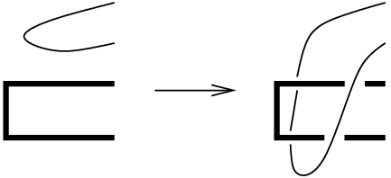
We now have a map, which we also write as $\psi$ , from cords of $K$ to $\mathcal{A}_{2n}/\mathcal{I}_{B}^{\operatorname{plat}}$ , which satisfies the skein relations (1), (2). (Any skein relation involving one of the segments $L_{j}\times\{0\}$ or $L_{j}\times\{1\}$ can be isotoped to one which involves a section of $B$ instead.) To ensure that the map is well-defined, we still need to check that the particular isotopy from a cord of $K$ to a cord in $D\times(0,1)$ is irrelevant. That is, the isotopy shown in Figure 7 should not affect the value of $\psi$ . (There is a similar isotopy around $L_{j}\times\{1\}$ instead of $L_{j}\times\{0\}$ , which can be dealt with similarly.)

In the projection to $(D,P)$ , the isotopy pictured in Figure 7 corresponds to moving a segment of a cord on one side of $L_{j}$ across to the other side, ie, passing this segment through the points $p_{2j-1}$ and $p_{2j}$ . Now we have the following chain of equalities in $\mathcal{A}_{2n}/\mathcal{I}_{B}^{\operatorname{plat}}$ :

$\displaystyle\psi(\raisebox{-18.7898pt}{\includegraphics[height]{figures/loop1.eps}})$	$\displaystyle=$	$\displaystyle-\psi(\raisebox{-18.7898pt}{\includegraphics[height]{figures/loop2.eps}})-\psi(\raisebox{-18.7898pt}{\includegraphics[height]{figures/loop3.eps}})\psi(\raisebox{-18.7898pt}{\includegraphics[height]{figures/loop4.eps}})$
	$\displaystyle=$	$\displaystyle\psi(\raisebox{-18.7898pt}{\includegraphics[height]{figures/loop5.eps}})-\psi(\raisebox{-18.7898pt}{\includegraphics[height]{figures/loop3.eps}})\psi(\raisebox{-18.7898pt}{\includegraphics[height]{figures/loop4.eps}})+\psi(\raisebox{-18.7898pt}{\includegraphics[height]{figures/loop6.eps}})\psi(\raisebox{-18.7898pt}{\includegraphics[height]{figures/loop7.eps}})$
	$\displaystyle=$	$\displaystyle\psi(\raisebox{-18.7898pt}{\includegraphics[height]{figures/loop5.eps}})$

where the dotted line represents $L_{j}$ , and the last equality holds by the definition of $\mathcal{I}_{B}^{\operatorname{plat}}$ . Hence the value of $\psi$ is unchanged under the isotopy of Figure 7.

To summarize, we have a map from cords of $K$ , modulo homotopy and skein relations, to $\mathcal{A}_{2n}/\mathcal{I}_{B}^{\operatorname{plat}}$ . By construction, this induces an isomorphism between the cord ring of $K$ and $\mathcal{A}_{2n}/\mathcal{I}_{B}^{\operatorname{plat}}$ , as desired. ∎

The argument of Theorem 4.1 also gives a plat description of $HC_{0}^{\operatorname{ab}}(K)$ .

Corollary 4.2.

$HC_{0}^{\operatorname{ab}}(K)$ can be obtained from $HC_{0}(K)\cong\mathcal{A}_{2n}/\mathcal{I}_{B}^{\operatorname{plat}}$ by further quotienting by $a_{ij}-a_{ji}$ for all $i,j$ and abelianizing. The result can be viewed as a quotient of the polynomial ring $\mathbb{Z}[\{a_{ij}|1\leq i<j\leq n\}]$ .

4.2 Two-bridge knots

For two-bridge knots, Theorem 4.1 implies that $HC_{0}$ has a particularly simple form. In particular, $HC_{0}$ is a quotient of $\mathcal{A}_{2}=\mathbb{Z}\langle a_{12},a_{21}\rangle$ ; in this quotient, it turns out that $a_{12}=a_{21}$ , so that $HC_{0}$ is a quotient of a polynomial ring $\mathbb{Z}[x]$ . The main result of this section shows that for two-bridge knots, $HC_{0}$ is actually determined by the knot’s determinant.

We recall some notation from [7]. If $K$ is a knot, $\Delta_{K}(t)$ denotes the Alexander polynomial of $K$ as usual, and $|\Delta_{K}(-1)|$ is the determinant of $K$ . Define the sequence of polynomials $\{p_{m}\in\mathbb{Z}[x]\}$ by $p_{0}(x)=2-x$ , $p_{1}(x)=x-2$ , $p_{m+1}(x)=xp_{m}(x)-p_{m-1}(x)$ .

Theorem 4.3.

If $K$ is a $2$ –bridge knot, then

HC_{0}(K)\cong HC_{0}^{\operatorname{ab}}(K)\cong\mathbb{Z}[x]/(p_{(|\Delta_{K}(-1)|+1)/2}(x)).

This generalizes [7, Proposition 7.3]. Also compare this result to [7, Theorem 6.13], which states that for any knot $K$ , there is a surjection from $HC_{0}(K)$ to $\mathbb{Z}[x]/(p_{(n(K)+1)/2}(x))$ , where $n(K)$ is the largest invariant factor of the first homology of the double branched cover of $K$ .

Before we can prove Theorem 4.3, we need to recall some results (and more notation) from [7], and establish a few more lemmas. Define the sequence $\{q_{m}\in\mathbb{Z}[x]\}$ by $q_{0}(x)=-2$ , $q_{1}(x)=-x$ , $q_{m+1}(x)=xq_{m}(x)-q_{m-1}(x)$ ; this recursion actually defines $q_{m}$ for all $m\in\mathbb{Z}$ , and $q_{-m}=q_{m}$ . The Burau representation of $B_{n}$ with $t=-1$ is given as follows: ${\operatorname{Bur}_{\sigma_{k}}}$ is the linear map on $\mathbb{Z}^{n}$ whose matrix is the identity, except for the $2\times 2$ submatrix formed by the $k,k+1$ rows and columns, which is $\left(\begin{smallmatrix}2&1\\ 1&0\end{smallmatrix}\right)$ . This extends to a representation which sends $B\in B_{n}$ to ${\operatorname{Bur}_{B}}$ . If $B$ is a braid, let $\hat{B}$ denote the braid obtained by reversing the word which gives $B$ .

Lemma 4.4.

[7]\quaFor $B\in B_{n}$ and $v\in\mathbb{Z}^{n}$ , if we set $a_{ij}=q_{v_{i}-w_{j}}$ for all $i,j$ , then $\phi_{B}(a_{ij})=q_{({\operatorname{Bur}_{\hat{B}}}v)_{i}-({\operatorname{Bur}_{\hat{B}}}v)_{j}}$ for all $i,j$ .

Let $K$ be a $2$ –bridge knot; then $K$ is the plat closure of some braid in $B_{4}$ of the form $B=\sigma_{2}^{-a_{1}}\sigma_{1}^{b_{1}}\sigma_{2}^{-a_{2}}\cdots\sigma_{1}^{b_{k}}\sigma_{2}^{-a_{k+1}}$ . As usual, we can then associate to $K$ the continued fraction

\frac{m}{n}=a_{1}+\frac{1}{b_{1}}\!\!\begin{array}[]{l}\\ +\end{array}\!\!\frac{1}{a_{2}}\!\!\begin{array}[]{l}\\ +\,\cdots\,+\end{array}\!\!\frac{1}{b_{k}}\begin{array}[]{l}\\ +\end{array}\!\!\frac{1}{a_{k+1}}\,,

where $\gcd(m,n)=1$ and $n>0$ .

Lemma 4.5.

For $B,m,n$ as above, we have ${\operatorname{Bur}_{B}}\left(\begin{smallmatrix}0\\ 0\\ 1\\ 1\end{smallmatrix}\right)=\left(\begin{smallmatrix}-n+1\\ m-n+1\\ m+1\\ 1\end{smallmatrix}\right).$

Proof.

We can compute that

\textstyle{{\operatorname{Bur}_{\sigma_{1}}}\left(\begin{smallmatrix}-n+1\\ m-n+1\\ m+1\\ 1\end{smallmatrix}\right)=\left(\begin{smallmatrix}-m-n+1\\ -n+1\\ m+1\\ 1\end{smallmatrix}\right)}\hskip 10.84006pt\textrm{and}\hskip 10.84006pt\textstyle{{\operatorname{Bur}_{\sigma_{2}^{-1}}}\left(\begin{smallmatrix}-n+1\\ m-n+1\\ m+1\\ 1\end{smallmatrix}\right)=\left(\begin{smallmatrix}-n+1\\ m+1\\ m+n+1\\ 1\end{smallmatrix}\right).}

The lemma follows easily by induction. ∎

We present one final lemma about the polynomials $p_{k}$ and $q_{k}$ . For any $k,m$ , define $r_{k,m}=q_{k}-q_{k-m}$ .

Lemma 4.6.

If $m>0$ is odd and $\gcd(m,n)=1$ , then $\gcd(r_{m,m},r_{n,m})=p_{(m+1)/2}$ .

Proof.

We first note that $r_{m-k,m}=-r_{k,m}$ and $r_{2k-l,m}-r_{l,m}-q_{l-k}r_{k,m}=0$ for all $k,l,m$ ; the first identity is obvious, while the second is an easy induction (or use Lemma 6.14 from [7]). It follows that $\gcd(r_{k,m},r_{l,m})$ is unchanged if we replace $(k,l)$ by any of $(l,k)$ , $(k,m-l)$ , $(l,2k-l)$ .

Now consider the operation which replaces any ordered pair $(k,l)$ for $k,l>m/2$ with: $(l,2l-k)$ if $k\geq l$ and $2l-k>m/2$ ; $(l,m-2l+k)$ if $k\geq l$ and $2l-k<m/2$ ; $(k,2k-l)$ if $k<l$ and $2k-l>m/2$ ; $(k,m-2k+l)$ if $k<l$ and $2k-l<m/2$ . This operation preserves $\gcd(r_{k,m},r_{l,m})$ and $\gcd(2k-m,2l-m)$ , as well as the condition $k,l>m/2$ ; it also strictly decreases $\max(k,l)$ unless $k=l$ .

We can now use a descent argument, beginning with the ordered pair $(m,n)$ and performing the operation repeatedly until we obtain a pair of the form $(k,k)$ . We then have $2k-m=\gcd(2m-n,m)=1$ and $\gcd(r_{m,m},r_{n,m})=r_{k,m}$ . The lemma now follows from the fact, established by induction, that $r_{(m+1)/2,m}=p_{(m+1)/2}$ . ∎

Proof of Theorem 4.3.

As usual, we assume that $K$ is the plat closure of $B\in B_{4}$ ; it is then also the case that $K$ is the plat closure of $\hat{B}$ . Let $m/n$ be the continued fraction associated to $K$ , and note that $|\Delta_{K}(-1)|=m$ .

By Theorem 4.1, $HC_{0}(K)$ is a quotient of $\mathcal{A}_{4}$ , and in this quotient, we can set $a_{12}=a_{21}=a_{34}=a_{43}=-2$ , $a_{13}=a_{14}=a_{23}=a_{24}$ , and $a_{31}=a_{41}=a_{32}=a_{42}$ .

We first compute $HC_{0}^{\operatorname{ab}}(K)$ . Here we can further set $a_{13}=a_{31}=:-x$ . Then we have $a_{ij}=q_{v_{i}-v_{j}}$ , where $v$ is the vector $(0,0,1,1)$ . By Lemma 4.4, we have $\phi_{\hat{B}}(a_{ij})=q_{({\operatorname{Bur}_{B}}v)_{i}-({\operatorname{Bur}_{B}}v)_{j}}$ ; by Lemma 4.5, we conclude the matrix identity:

(\phi_{\hat{B}}(a_{ij}))=\left(\begin{array}[]{cc|cc}q_{0}&q_{-m}&q_{-m-n}&q_{-n}\\ q_{m}&q_{0}&q_{-n}&q_{m-n}\\ \hline\cr q_{m+n}&q_{n}&q_{0}&q_{m}\\ q_{n}&q_{-m+n}&q_{-m}&q_{0}\end{array}\right)

Here we have divided the matrix into $2\times 2$ blocks for clarity. By Theorem 4.1, the relations defining $HC_{0}(K)$ then correspond to equating the entries within each block. In other words, since $q_{-k}=q_{k}$ for all $k$ , we have

HC_{0}(K)\cong\mathbb{Z}[x]/(q_{m}-q_{0},q_{m+n}-q_{n},q_{n}-q_{n-m})=\mathbb{Z}[x]/(r_{m,m},r_{m+n,m},r_{n,m}).

We may assume without loss of generality that $m>0$ (otherwise replace $m$ by $-m$ ); furthermore, $m$ is odd since $K$ is a knot rather than a two-component link. By Lemma 4.6, we can then conclude that $HC_{0}(K)\cong\mathbb{Z}[x]/(p_{(m+1)/2})=\mathbb{Z}[x]/(p_{(|\Delta_{K}(-1)|+1)/2})$ .

The computation of $HC_{0}(K)$ rather than $HC_{0}^{\operatorname{ab}}(K)$ is very similar but becomes notationally more complicated. Set $a_{13}=a_{1}$ and $a_{31}=a_{2}$ , so that $HC_{0}(K)$ is a quotient of $\mathbb{Z}\langle a_{1},a_{2}\rangle$ . As in Section 7.3 of [7], we define two sequences $\{q_{k}^{(1)},q_{k}^{(2)}\}$ by $q_{0}^{(1)}=q_{0}^{(2)}=-2$ , $q_{1}^{(1)}=a_{1}$ , $q_{1}^{(2)}=a_{2}$ , and $q_{m+1}^{(1)}=-a_{1}q_{m}^{(2)}-q_{m-1}^{(1)}$ , $q_{m+1}^{(2)}=-a_{2}q_{m}^{(1)}-q_{m-1}^{(2)}$ . Note that $q_{m}^{(1)}|_{a_{1}=a_{2}=-x}=q_{m}^{(2)}|_{a_{1}=a_{2}=-x}=q_{m}$ , and that each nonconstant monomial in $q_{m}^{(1)}$ (resp. $q_{m}^{(2)}$ ) begins with $a_{1}$ (resp. $a_{2}$ ).

In terms of $a_{1},a_{2}$ , the monomials appearing in $\phi_{\hat{B}}(a_{ij})$ look like $a_{1}a_{2}a_{1}\cdots$ or $a_{2}a_{1}a_{2}\cdots$ . Since $\phi_{\hat{B}}(a_{ij})$ projects to the appropriate polynomial $q_{k}$ if we set $a_{1}=a_{2}=-x$ , it readily follows that

(\phi_{\hat{B}}(a_{ij}))=\left(\begin{array}[]{cc|cc}q_{0}^{(r)}&q_{-m}^{(r)}&q_{-m-n}^{(r)}&q_{-n}^{(r)}\\ q_{m}^{(s)}&q_{0}^{(s)}&q_{-n}^{(s)}&q_{m-n}^{(s)}\\ \hline\cr q_{m+n}^{(1)}&q_{n}^{(1)}&q_{0}^{(1)}&q_{m}^{(1)}\\ q_{n}^{(2)}&q_{-m+n}^{(2)}&q_{-m}^{(2)}&q_{0}^{(2)}\end{array}\right)

where $(r,s)=(1,2)$ or $(2,1)$ . (The superscripts follow from an inspection of the permutation on the four strands induced by $\hat{B}$ .) To obtain $HC_{0}(K)$ from $\mathbb{Z}\langle a_{1},a_{2}\rangle$ , we quotient by setting the entries of each $2\times 2$ block equal to each other.

If we define $r_{k,m}^{(1)}=q_{k}^{(1)}-q_{k-m}^{(1)}$ , $r_{k,m}^{(2)}=q_{k}^{(2)}-q_{k-m}^{(2)}$ , $s_{k,m}^{(1)}=q_{k}^{(1)}-q_{k-m}^{(2)}$ , $s_{k,m}^{(2)}=q_{k}^{(2)}-q_{k-m}^{(1)}$ , then we have

r_{2l-k,m}^{(1)}-r_{k,m}^{(1)}-q_{k-l}^{(p)}r_{l,m}^{(1)}=0

for all $k,l,m$ , where $p=1$ or $2$ depending on the parity of $k-l$ , with similar relations for $r^{(2)}$ , $s^{(1)}$ , and $s^{(2)}$ . Using these identities and the descent argument of Lemma 4.6, we deduce (after a bit of work) that

HC_{0}(K)\cong\mathbb{Z}\langle a_{1},a_{2}\rangle/\langle r_{(m+1)/2,m}^{(1)},r_{(m+1)/2,m}^{(2)},s_{(m+1)/2,m}^{(1)},s_{(m+1)/2,m}^{(2)}\rangle.

It can be directly deduced at this point that $a_{1}=a_{2}$ in $HC_{0}(K)$ , whence we can argue as before, but we can circumvent this somewhat involved calculation by noting that we have now established that $HC_{0}(K)$ depends only on $m=|\Delta_{K}(-1)|$ . Since $T(2,2m-1)$ is a $2$ –bridge knot with determinant $m$ , it follows that $HC_{0}(K)$ is isomorphic to $HC_{0}(T(2,2m-1))$ , which is $\mathbb{Z}[x]/(p_{(m+1)/2})$ by [7, Proposition 7.2]. ∎

We conclude this section by noting that Theorem 4.1 and Corollary 4.2 are also useful for knots that are not $2$ –bridge. For instance, if $K$ has bridge number $3$ , then $HC_{0}^{\operatorname{ab}}(K)$ is a quotient of $\mathbb{Z}[a_{12},a_{13},a_{23}]$ , and can be readily computed in many examples, given Gröbner basis software and sufficient computer time. One can calculate, for example, that $HC_{0}^{\operatorname{ab}}(P(3,3,2))\cong\mathbb{Z}[x]/((x-1)p_{11})$ and $HC_{0}^{\operatorname{ab}}(P(3,3,-2))\cong\mathbb{Z}[x]/((x-1)p_{5})$ , where $P(p,q,r)$ is the $(p,q,r)$ pretzel knot. For other knots, such as $P(3,3,3)$ and $P(3,3,-3)$ , $HC_{0}^{\operatorname{ab}}$ is not a quotient of $\mathbb{Z}[x]$ . See also Section 5.2.

4.3 The cord ring in terms of a knot diagram

Here we give a description of the cord ring of a knot given any knot diagram, not necessarily a plat or a braid closure.

Suppose that we are given a knot diagram for $K$ with $n$ crossings. There are $n$ components of the knot diagram (ie, segments of $K$ between consecutive undercrossings), which we may label $1,\ldots,n$ . For any $i,j$ in $\{1,\ldots,n\}$ , we can define a cord $\gamma_{ij}$ of $K$ which begins at any point on component $i$ , ends at any point on component $j$ , and otherwise lies completely above the plane of the knot diagram. (In particular, away from a neighborhood of each endpoint, it lies above any crossings of the knot.) Such a cord is well-defined up to homotopy.

Any cord of $K$ can be expressed, via the skein relations, in terms of these cords $\gamma_{ij}$ ; imagine pushing the cord upwards while fixing its endpoints, using the skein relations if necessary, until the result consists of cords which lie completely above the plane of the diagram. The crossings in the knot diagram give relations in the cord ring. More precisely, consider a crossing whose overcrossing strand is component $i$ , and whose undercrossing strands are components $j$ and $k$ . For any $l$ , the cords $\gamma_{lj}$ and $\gamma_{lk}$ are obtained from one another by passing through component $i$ ; since the cord joining overcrossing to undercrossing is $\gamma_{ij}$ (which is homotopic to $\gamma_{ik}$ ), we have the skein relation $\gamma_{lj}+\gamma_{lk}+\gamma_{li}\cdot\gamma_{ij}=0$ . See Figure 8. Similarly, there are skein relations of the form $\gamma_{jl}+\gamma_{kl}+\gamma_{ji}\cdot\gamma_{il}=0$ .

Let $\mathcal{A}_{n}$ denote the usual tensor algebra, and set $a_{ii}=-2$ for all $i$ . Define $\mathcal{I}^{\operatorname{diagram}}_{K}\subset\mathcal{A}_{n}$ to be the ideal generated by the elements $a_{lj}+a_{lk}+a_{li}a_{ij}$ , $a_{jl}+a_{kl}+a_{ji}a_{il}$ , where $l=1,\ldots,n$ and $(i,j,k)$ ranges over all $n$ crossings of the knot diagram; as before, $i$ is the overcrossing strand and $j,k$ are the undercrossing strands. Then there is a map from the cord ring of $K$ to $\mathcal{A}_{n}/\mathcal{I}^{\operatorname{diagram}}_{K}$ given by sending $\gamma_{ij}$ to $a_{ij}$ for all $i,j$ . It is straightforward to check that this map is well-defined and an isomorphism. In particular, all skein relations in the cord ring follow from the skein relations mentioned above.

Proposition 4.7.

The cord ring of $K$ is isomorphic to $\mathcal{A}_{n}/\mathcal{I}^{\operatorname{diagram}}_{K}$ .

This result may seem impractical, because it expresses the cord ring of a knot with $n$ crossings as a ring with $n(n-1)$ generators. However, each relation generating $\mathcal{I}^{\operatorname{diagram}}_{K}$ allows us to express one generator in terms of three others, and this helps in general to eliminate the vast majority of these generators.

As an example, consider the usual diagram for a trefoil, and label the diagram components $1,2,3$ in any order. The crossing where $1$ is the overcrossing strand yields relations $-2+a_{13}+a_{12}a_{23}$ , $a_{21}-a_{23}$ , $a_{31}-2+a_{32}a_{23}$ , $-2+a_{31}+a_{32}a_{21}$ , $a_{12}-a_{32}$ , $a_{13}-2+a_{32}a_{23}$ . The other two crossings yield the same relations, but with indices cyclically permuted. In $\mathcal{A}_{n}/\mathcal{I}^{\operatorname{diagram}}_{K}$ , we conclude that $a_{12}=a_{32}=a_{31}=a_{21}=a_{23}=a_{13}$ , and the cord ring for the trefoil is $\mathbb{Z}[x]/(x^{2}+x-2)$ .

Among the three techniques we have discussed to calculate the cord ring (braid closure, plat, diagram), there are instances when the diagram technique is computationally easiest. In particular, using diagrams allows us to study the cord ring for a knot in terms of tangles contained in the knot.

5 Some geometric remarks

In this section, we discuss some geometric consequences of the cord ring construction. Section 5.1 relates the cord ring to binormal chords of a knot; Section 5.2 establishes a close connection between the abelian cord ring and the double branched cover of the knot; and Section 5.3 discusses some ways to extend the cord ring to other invariants.

5.1 Minimal chords

Here we apply the cord ring to deduce a lower bound on the number of minimal chords (see below for definition) of a knot in terms of the double branched cover of the knot. We will also indicate a conjectural way in which the entire knot DGA of [7] could be defined in terms of chords. Note that the results in this section are equally valid for links.

If we impose the usual metric on $\mathbb{R}^{3}$ , we can associate a length to any sufficiently well-behaved ( $L^{2}$ ) cord of a knot $K$ . Define a minimal chord¹¹ 1 Regarding the spelling: following a suggestion of D Bar-Natan, we have adopted the spelling “cord” in this paper so as to avoid confusion with the chords from the theory of Vassiliev invariants. In this case, however, a minimal cord is in fact a “chord,” that is, a straight line segment. to be a nontrivial cord which locally minimizes length. In other words, the embedding of $K$ in $\mathbb{R}^{3}$ gives a distance function $d\colon\thinspace S^{1}\times S^{1}\rightarrow\mathbb{R}_{\geq 0}$ , where $S^{1}$ parametrizes $K$ and $d$ is the usual distance between two points in $\mathbb{R}^{3}$ ; then a minimal chord is a local minimum for $d$ not lying on the diagonal of $S^{1}\times S^{1}$ . Clearly any minimal chord can be traversed in the opposite direction and remains a minimal chord; when counting minimal chords, we will identify minimal chords with their opposites and only count one from each pair. Minimal chords have previously been studied in the literature, especially in the context of the “thickness” or “ropelength” of a knot.

In the cord ring of $K$ , any cord can be expressed in terms of minimal chords. To see this, imagine a cord as a rubber band, and pull it taut while keeping its endpoints on $K$ . If the result is not a minimal chord, then it “snags” on the knot, giving a union of broken line segments; using the skein relation, we can express the result in terms of shorter cords, which we similarly pull taut, and so forth, until all that remains are minimal chords.

Proposition 5.1.

The number of minimal chords for any embedding $K\subset\mathbb{R}^{3}$ is at least the minimal possible number of generators of the ring $HC_{0}^{\operatorname{ab}}(K)$ .

As a consequence, for instance, any embedding of $P(3,3,3)$ , $P(3,3,-3)$ , or $3_{1}\#3_{1}$ in $\mathbb{R}^{3}$ has at least two minimal chords.

A similar result which is slightly weaker, but generally easier to apply, involves the linearized group $HC_{0}^{\operatorname{lin}}$ introduced in [7]. We first note the following expression for $HC_{0}^{\operatorname{lin}}$ in terms of cords, which is an immediate consequence of Theorem 1.3.

Proposition 5.2.

The group $HC_{0}^{\operatorname{lin}}(K)$ is the free abelian group generated by homotopy classes of cords of $K$ , modulo the relations:

\raisebox{-12.28577pt}{\includegraphics[width]{figures/skein12.eps}}+\raisebox{-12.28577pt}{\includegraphics[width]{figures/skein11.eps}}-2\raisebox{-12.28577pt}{\includegraphics[width]{figures/skein13.eps}}-2\raisebox{-12.28577pt}{\includegraphics[width]{figures/skein14.eps}}=0

\raisebox{-12.28577pt}{\includegraphics[width]{figures/skein21.eps}}=0

The argument used to establish Proposition 5.1 now yields the following.

Proposition 5.3.

The number of minimal chords for an embedding of $K$ is at least the minimal possible number of generators of the group $HC_{0}^{\operatorname{lin},\operatorname{ab}}(K)$ .

We can use Proposition 5.3 to give a lower bound on the number of minimal chords of a knot which involves only “classical” topological information, without reference to the cord ring.

Corollary 5.4.

If $K$ is a knot, let $m(K)$ be the number of invariant factors of the abelian group $H_{1}(\Sigma_{2}(K))$ , where $\Sigma_{2}(K)$ is the double branched cover of $S^{3}$ over $K$ . Then the number of minimal chords for an embedding of $K$ is at least $\binom{m(K)+1}{2}$ .

Proof.

By [7, Proposition 7.11] there is a surjection of groups from $HC_{0}^{\operatorname{lin},\operatorname{ab}}(K)$ to $\operatorname{Sym}^{2}(H_{1}(\Sigma_{2}(K)))$ . It is easy to see that the minimal number of generators of $\operatorname{Sym}^{2}(H_{1}(\Sigma_{2}(K)))$ is $\binom{m(K)+1}{2}$ . ∎

As a result of Corollary 5.4, we can demonstrate that there are knot types for which the number of minimal chords must be arbitrarily large.

Corollary 5.5.

Let $K$ be a knot, and $\overline{K}$ its mirror. The number of minimal chords of an embedding of the knot $\#^{m_{1}}K\#^{m_{2}}\overline{K}$ is at least $\binom{m_{1}+m_{2}+1}{2}$ .

Proof.

We have $H_{1}(\Sigma_{2}(\#^{m_{1}}K\#^{m_{2}}\overline{K}))\cong\oplus^{m_{1}+m_{2}}H_{1}(\Sigma_{2}(K))$ . ∎

It is not hard to show that any knot with bridge number $k$ has an embedding with exactly $\binom{k}{2}$ minimal chords. Hence Corollary 5.5 gives a sharp bound whenever $K$ is $2$ –bridge. To the author’s knowledge, it is an open problem to find sharp lower bounds for the number of minimal chords for a general knot.

The fact that $HC_{0}(K)$ can be expressed in terms of minimal chords suggests that there might be a similar expression for the entire knot DGA (see [7] for definition), of which $HC_{0}$ is the degree $0$ homology. Here we sketch a conjectural formulation for the knot DGA in terms of chords.

Let a segment chord of $K$ be a cord consisting of a directed line segment; note that the space of segment chords is parametrized by $S^{1}\times S^{1}$ , minus a $1$ –dimensional subset $C$ corresponding to segments which intersect $K$ in an interior point. Generically, there are finitely many binormal chords of $K$ , which are normal to $K$ at both endpoints; these are critical points of the distance function $d$ on $S^{1}\times S^{1}$ , and include minimal chords. The critical points of $d$ then consist of binormal chords, along with the diagonal in $S^{1}\times S^{1}$ .

Let $\mathcal{A}$ denote the tensor algebra generated by binormal chords of $K$ , with grading given by setting the degree of a binormal chord to be the index of the corresponding critical point of $d$ . We can define a differential on $\mathcal{A}$ using gradient flow trees, as we now explain.

In the present context, a gradient flow tree consists of negative gradient flow for $d$ on $S^{1}\times S^{1}$ , except that the flow is allowed to bifurcate at a point of $C$ , by jumping from this point $(t_{1},t_{2})$ to the two points $(t_{1},t_{3}),(t_{3},t_{2})$ corresponding to the segment chords into which $K$ divides the chord $(t_{1},t_{2})$ . (See Figure 9.) Now consider binormal chords $a_{i},a_{j_{1}},\ldots,a_{j_{k}}$ (not necessarily distinct), and look at the moduli space $\mathcal{M}(a_{i};a_{j_{1}},\ldots,a_{j_{k}})$ of gradient flow trees beginning at $a_{i}$ and ending at $a_{j_{1}},\ldots,a_{j_{k}}$ , possibly along with some ending points on the diagonal of $S^{1}\times S^{1}$ . To each such tree, we associate the monomial $(-2)^{p}a_{j_{1}}\cdots a_{j_{k}}$ , where $p$ is the number of endpoints on the diagonal, and the order of the $a_{j_{l}}$ ’s is determined in a natural way by the bifurcations. The expected dimension of $\mathcal{M}(a_{i};a_{j_{1}},\ldots,a_{j_{k}})$ turns out to be $\deg a_{i}-\sum\deg a_{j_{l}}-1$ ; we then define the differential of $a_{i}$ to be the sum over all trees in $0$ –dimensional moduli spaces of the monomial associated to the tree.

We conjecture that the resulting differential graded algebra $(\mathcal{A},\partial)$ is stable tame isomorphic to the knot DGA from [7], at least over $\mathbb{Z}_{2}$ ; establishing an equivalence over $\mathbb{Z}$ would entail sorting through orientation issues on the above moduli spaces, à la Morse homology. The knot DGA conjecturally represents a relative contact homology theory, as described in [7, Section 3], which bears a striking resemblance to the DGA described above. In particular, the DGA of the contact homology is generated by binormal chords, and the differential is also given by gradient flow trees. However, the assignment of grading in the two DGAs is different in general, as is the differential.

We remark that it should be possible to bound the total number of binormal chords for a knot by examining the full knot contact homology $HC_{*}(K)$ , similarly to minimal chords and $HC_{0}$ .

5.2 Cords and $\Sigma_{2}(K)$

In [7], it was demonstrated that knot contact homology has a close relation to the double branched cover $\Sigma_{2}(K)$ of $S^{3}$ over the knot $K$ . Cords can be used to elucidate this relationship, as we will now see. Recall that the ( $SL_{2}(\mathbb{C})$ ) character variety of $\Sigma_{2}(K)$ is the variety of characters of $SL_{2}(\mathbb{C})$ representations of $\pi_{1}(\Sigma_{2}(K))$ .

Proposition 5.6.

There is a map over $\mathbb{C}$ from $HC_{0}^{\operatorname{ab}}(K)\otimes\mathbb{C}$ to the coordinate ring of the character variety of $\Sigma_{2}(K)$ .

Proof.

Given an $SL_{2}(\mathbb{C})$ character $\chi\colon\thinspace\pi_{1}(\Sigma_{2}(K))\to\mathbb{C}$ , we wish to produce a map $HC_{0}^{\operatorname{ab}}(K)\otimes\mathbb{C}\to\mathbb{C}$ . Note that $\chi$ satisfies $\chi(e)=2$ , $\chi(g^{-1})=\chi(g)$ , and $\chi(g_{1}g_{2})+\chi(g_{1}^{-1}g_{2})=\chi(g_{1})\chi(g_{2})$ for all $g,g_{1},g_{2}\in\pi_{1}(\Sigma_{2}(K))$ .

Any (unoriented) cord $\gamma$ of $K$ has two lifts to $\Sigma_{2}(K)$ with the same endpoints; arranging these lifts head-to-tail gives an element $\tilde{\gamma}$ of $\pi_{1}(\Sigma_{2}(K))$ which is unique up to conjugation and inversion. In particular, $\chi(\tilde{\gamma})$ is well defined. We claim that the map sending each cord $\gamma$ to $-\chi(\tilde{\gamma})$ descends to the desired map $HC_{0}^{\operatorname{ab}}(K)\otimes\mathbb{C}\to\mathbb{C}$ ; this simply entails checking the skein relations in the definition of the cord ring (Definition 1.2). The second skein relation (2) is preserved since $\chi(e)=2$ . As for the first relation (1), label the cords depicted in (1) by $\gamma_{3},\gamma_{4},\gamma_{1},\gamma_{2}$ in order, so that the relation reads $\gamma_{3}+\gamma_{4}+\gamma_{1}\gamma_{2}=0$ . If we choose the base point for $\pi_{1}(\Sigma_{2}(K))$ to be the point on the knot depicted in the skein relation, then $\tilde{\gamma}_{3}$ and $\tilde{\gamma}_{4}$ are conjugate to $\tilde{\gamma}_{1}\tilde{\gamma}_{2}$ and $\tilde{\gamma}_{1}^{-1}\tilde{\gamma}_{2}$ in some order. Since $\chi(\tilde{\gamma}_{1}\tilde{\gamma}_{2})+\chi(\tilde{\gamma}_{1}^{-1}\tilde{\gamma}_{2})=\chi(\tilde{\gamma}_{1})\chi(\tilde{\gamma}_{2})$ , (1) is preserved. ∎

If $K$ is two-bridge, then $\Sigma_{2}(K)$ is a lens space and $\pi_{1}(\Sigma_{2}(K))\cong\mathbb{Z}/n$ where $n=\Delta_{K}(-1)$ . In this case, all $SL_{2}(\mathbb{C})$ representations of $\pi_{1}(\Sigma_{2}(K))$ are reducible, with character on the generator of $\mathbb{Z}_{n}$ given by $\omega^{k}+\omega^{-k}$ where $\omega$ is a primitive $n$ -th root of unity and $0\leq k\leq n-1$ . It follows that the coordinate ring of the character variety of $\Sigma_{2}(K)$ is $\mathbb{C}[x]/(p_{(n+1)/2}(x))$ with $p_{(n+1)/2}(x)=\prod_{k=0}^{(n-1)/2}\left(x-\omega^{k}-\omega^{-k}\right)$ . This is precisely the polynomial defined inductively in Section 4.2. It follows from Theorem 4.3 that the map in Proposition 5.6 is an isomorphism when $K$ is two-bridge.

In fact, a number of calculations on small knots lead us to propose the following.

Conjecture 5.7.

The map in Proposition 5.6 is always an isomorphism; the complexified cord ring $HC_{0}^{\operatorname{ab}}(K)\otimes\mathbb{C}$ is precisely the coordinate ring of the character variety of $\Sigma_{2}(K)$ .

In general, the surjection $HC_{0}^{\operatorname{ab}}(K)\twoheadrightarrow\mathbb{Z}[x]/(p_{(n(K)+1)/2})$ from [7, Theorem 7.1], where $n(K)$ is the largest invariant factor of $H_{1}(\Sigma_{2}(K))$ , can be seen via the approach of Proposition 5.6 by restricting to reducible representations. Proving surjectivity from this viewpoint takes a bit more work, though.

We can also use cords to see the surjection $HC_{0}^{\operatorname{lin},\operatorname{ab}}(K)\twoheadrightarrow\operatorname{Sym}^{2}(H_{1}(\Sigma_{2}(K)))$ from [7, Proposition 7.11], which was cited in the proof of Corollary 5.4 above. Consider $H_{1}(\Sigma_{2}(K))$ as a $\mathbb{Z}$ –module, with group multiplication given by addition. Given a cord of $K$ , we obtain an element of $H_{1}(\Sigma_{2}(K))$ , as in the proof of Proposition 5.6, defined up to multiplication by $\pm 1$ ; the square of this element gives a well-defined element of $\operatorname{Sym}^{2}(H_{1}(\Sigma_{2}(K)))$ . The fact that this map descends to $HC_{0}^{\operatorname{lin},\operatorname{ab}}(K)$ is the identity $(x+y)^{2}+(x-y)^{2}-2x^{2}-2y^{2}=0$ . Again, proving that this map is surjective takes slightly more work.

5.3 Extensions of the cord ring

We briefly mention here a couple of extensions of the knot cord ring. These each produce new invariants which may be of interest.

One possible extension is to define a cord ring for any knot in any $3$ –manifold, in precisely the same way as in $\mathbb{R}^{3}$ . If the $3$ –manifold and the knot are sufficiently well-behaved (eg, no wild knots), it seems likely that the cord ring will always be finitely generated. The cord ring would be a natural candidate for the degree $0$ portion of the appropriate relative contact homology [7, Section 3]. It would be interesting to construct tools to compute the cord ring in general, akin to the methods used in [7] and this paper. See also the Appendix.

As another extension, we note that the definition of the cord ring makes sense not only for knots, but also for graphs embedded in $\mathbb{R}^{3}$ , including singular knots. It is clear for topological reasons that the cord ring is invariant under neighborhood equivalence; recall that two embedded graphs are neighborhood equivalent if small tubular neighborhoods of each are ambient isotopic.

Proposition 5.8.

The cord ring is an invariant of graphs embedded in $\mathbb{R}^{3}$ , modulo neighborhood equivalence.

By direct calculation, one can show that the cord ring is a nontrivial invariant for graphs of higher genus than knots. For instance, the graph consisting of the union of a split link and a path connecting its components has cord ring which surjects onto the cord ring of each component of the link. By contrast, the figure eight graph (or the theta graph), like the unknot, has trivial cord ring $\mathbb{Z}$ .

The graph cord ring can be applied to tunnel numbers of knots, via the observation that any graph whose complement is a handlebody has trivial cord ring. This can be used to compute lower bounds for the tunnel numbers of some knots, but the process is somewhat laborious.

Appendix: The cord ring and fundamental groups

In this appendix we show that the cord ring is determined by the fundamental group and peripheral structure of a knot. We then introduce a generalization of the cord ring to any codimension $2$ submanifold of any manifold and derive a homotopy-theoretic formulation in this more general case. As an application, we show that the cord ring gives a nontrivial invariant for embeddings of $S^{2}$ in $S^{4}$ .

Assume that we are given a knot $K\subset S^{3}$ ; it is straightforward to modify the constructions here to links. Let $N(K)$ denote a regular neighborhood of $K$ and let $M=S^{3}\setminus\operatorname{int}(N(K))$ denote the knot exterior. Write $G=\pi_{1}(M)$ , and let $P$ be the image of $\pi_{1}(\partial N(K))$ in $G$ ; define $\mathcal{C}(G,P)=P\backslash G/P$ , and write $[g]$ for the image of $g\in G$ in $\mathcal{C}(G,P)$ .

Lemma A.1.

The set $\mathcal{C}_{K}$ of homotopy classes of cords of $K$ is identical to $\mathcal{C}(G,P)$ .

Proof.

As in the proof of the Van Kampen theorem, it is easy to see that there is a one-to-one correspondence between homotopy classes of cords for $K$ and homotopy classes of cords in the knot exterior $M$ , where a cord in $M$ is a continuous path $\alpha\colon\thinspace[0,1]\to M$ with $\alpha^{-1}(\partial M)=\{0,1\}$ . We will identify the latter set of homotopy classes with $P\backslash G/P$ .

Fix a base point $x_{0}$ in $\partial M$ . Given a cord $\alpha$ in $M$ , we pick paths $\beta$ and $\gamma$ in $\partial M$ joining $x_{0}$ to $\alpha(0)$ and $\alpha(1)$ . We associate to $\alpha$ the equivalence class $[\beta\alpha\gamma^{-1}]\in P\backslash G/P$ . This is clearly independent of the choice of $\beta$ and $\gamma$ . Furthermore, homotopic cords give the same element of $P\backslash G/P$ , because a family of cords can be given a continuous family of paths $\beta$ , $\gamma$ . Hence we have a map from the set of cords of $M$ to $P\backslash G/P$ .

To construct the inverse of this map, observe that each element in $G$ has a representative which does not intersect $\partial M$ in its interior, and hence gives a cord which is unique up to homotopy; in addition, for any $g\in G$ and $h,k\in P$ , $g$ and $hgk$ give homotopic cords. This completes the proof of the lemma. ∎

Using Lemma A.1, we can reformulate the definition of the cord ring in group-theoretic terms. Let $\mathcal{A}(G,P)$ be the tensor algebra freely generated by the set $\mathcal{C}(G,P)$ , let $\mu\in G$ denote the homotopy class of the meridian of $K$ , and let $I(\mu)$ be the ideal in $\mathcal{A}(G,P)$ generated by the “skein relations”

[\alpha\mu\beta]+[\alpha\beta]+[\alpha]\cdot[\beta],~~~~~\alpha,\beta\in G,

and $[e]+2$ , where $e=1\in G$ .

Proposition A.2.

$\mathcal{A}(G,P)/I(\mu)$ is the cord ring of the knot $K$ .

Proof.

The skein relations generating $I(\mu)$ are simply the homotopy-theoretic versions of the skein relations in the cord ring. ∎

Note that the above construction associates a ring to any triple $(G,P,\mu)$ , where $G$ is a group, $P$ a subgroup, and $\mu$ an element of $P$ . Such a triple is naturally associated to any codimension $2$ embedding $K\subset M$ of manifolds; we will be more precise presently. In this general setting, we can introduce a cord ring which agrees with $\mathcal{A}(G,P)/I(\mu)$ , and which specializes to the usual cord ring for knots in $S^{3}$ .

Definition A.3.

Let $K\subset M$ be a codimension $2$ submanifold. A cord of $K$ is a continuous path $\gamma\colon\thinspace[0,1]\rightarrow M$ with $\gamma^{-1}(K)=\{0,1\}$ . A near homotopy of cords is a continuous map $\eta\colon\thinspace[0,1]\times[0,1]\rightarrow M$ with $\eta^{-1}(K)=([0,1]\times\{0\})\cup([0,1]\times\{1\})\cup\{(t_{0},s_{0})\}$ , for some $(t_{0},s_{0})\in(0,1)\times(0,1)$ such that $\eta$ is transverse to $K$ in a neighborhood of $(t_{0},s_{0})$ .

Less formally, a near homotopy of cords is a homotopy of cords, except for one point in the homotopy where the cord breaks into two.

Just as for knots in $S^{3}$ , let $\mathcal{C}_{K}$ denote the set of homotopy classes of cords of $K$ , and let $\mathcal{A}_{K}$ be the tensor algebra freely generated by $\mathcal{C}_{K}$ . To each near homotopy of cords, we can associate an element in $\mathcal{A}_{K}$ , namely $[\gamma_{0}]+[\gamma_{1}]+[\gamma_{2}]\cdot[\gamma_{3}]$ , where $\gamma_{0},\gamma_{1},\gamma_{2},\gamma_{3}$ are the cords of $K$ corresponding to $\eta(\{0\}\times[0,1])$ , $\eta(\{1\}\times[0,1])$ , $\eta(\{t_{0}\}\times[0,s_{0}])$ , $\eta(\{t_{0}\}\times[s_{0},1])$ , respectively. Now define $\mathcal{I}_{K}$ to be the ideal in $\mathcal{A}_{K}$ generated by the elements associated to all possible near homotopies, along with the element $[e]+2$ , where $e$ represents the homotopy class of a contractible cord. (For a knot in $\mathbb{R}^{3}$ , this agrees with the skein-relation definition of $\mathcal{I}_{K}$ used to formulate the original cord ring.)

Definition A.4.

The cord ring of $K\subset M$ is $\mathcal{A}_{K}/\mathcal{I}_{K}$ .

It is clear that the cord ring is an invariant under isotopy. We have seen that, for knots in $S^{3}$ , the cord ring can be written group-theoretically, in terms of the peripheral structure of the knot group. A similar expression can be given for the cord ring of a general codimension $2$ submanifold $K\subset M$ . Let $N(K)$ denote a tubular neighborhood of $K$ in $M$ ; its boundary is a circle bundle over $K$ . Set $G=\pi_{1}(M\setminus K)$ with base point $p$ on $\partial N(K)$ , $P=i_{*}\pi_{1}(\partial N(K))$ where $i$ is the inclusion $\partial N(K)\hookrightarrow M\setminus K$ , and $\mu$ equals the homotopy class of the $S^{1}$ fiber of $\partial N(K)$ containing $p$ .

Proposition A.5.

For any codimension $2$ submanifold $K$ , the cord ring of $K$ is isomorphic to $\mathcal{A}(G,P)/I(\mu)$ .

Proof.

Completely analogous to the proof for knots in $S^{3}$ . ∎

We now consider a particular example of the cord ring, for embeddings of $S^{2}$ in $S^{4}$ . Recall that any knot in $S^{3}$ yields a “spun knot” $2$ –sphere in $S^{4}$ ; see, eg, [8].

Proposition A.6.

The cord ring distinguishes between the unknotted $S^{2}$ in $S^{4}$ and the spun knot obtained from any knot in $S^{3}$ with nontrivial cord ring (in particular, any knot with determinant not equal to $1$ ).

Proof.

In the case of the unknotted $S^{2}$ , $G=P=\mathbb{Z}$ and hence the cord ring is trivial. On the other hand, suppose that $K$ is a knot with nontrivial cord ring. For the spun knot obtained from $K$ , $G$ is $\pi_{1}(S^{3}\setminus K)$ , $\mu$ is the element corresponding to the meridian of $K$ , and $P$ is the subgroup of $G$ generated by $\mu$ . It follows that the cord ring of the spun knot surjects onto the cord ring for $K$ , and hence is nontrivial. ∎

Thus the cord ring gives a nontrivial invariant for a large class of $2$ –knots in $S^{4}$ .

Just as the cord ring for knots in $\mathbb{R}^{3}$ should give the zero-dimensional relative contact homology of a certain Legendrian torus in $ST^{*}\!\mathbb{R}^{3}$ , we believe that the cord ring in general should correspond to a zero-dimensional contact homology. Recall from, eg, [7] that any submanifold $K\subset M$ gives a Legendrian submanifold $LK$ of the contact manifold $ST^{*}\!M$ given by the unit conormal bundle to $K$ .

Conjecture A.7.

For any codimension $2$ submanifold $K\subset M$ , the cord ring of $K$ is the zero-dimensional relative contact homology of $LK$ in $ST^{*}\!M$ .

Another natural direction of inquiry is to consider higher-dimensional contact homology for knots. Viterbo ([10], see also [1, 9]) has shown that the Floer homology of the tangent bundle of a manifold is the cohomology of its loop space. Here we have shown how the zero-dimensional contact homology of a knot can similarly be determined in terms of the algebraic topology of the space of cords. It seems possible that higher-dimensional contact homology may have a description analogous to our description, except that one takes into account not just the homotopy classes of cords, but the full homotopy type of the space of cords.

References

[1] A Abbondandolo, M Schwarz, On the Floer homology of cotangent bundles, Comm. Pure Appl. Math. to appear
[2] S J Bigelow, Braid groups are linear, J. Amer. Math. Soc. 14 (2001) 471–486 \MR1815219
[3] J S Birman, Braids, links, and mapping class groups, Princeton University Press, Princeton, N.J. (1974) \MR0375281
[4] S P Humphries, An approach to automorphisms of free groups and braids via transvections, Math. Z. 209 (1992) 131–152 \MR1143219
[5] D Krammer, The braid group $B_{4}$ is linear, Invent. Math. 142 (2000) 451–486 \MR1804157
[6] W Magnus, Rings of Fricke characters and automorphism groups of free groups, Math. Z. 170 (1980) 91–103 \MR558891
[7] L Ng, Knot and braid invariants from contact homology. I, \gtref920058247297 \MRMR2116316
[8] D Rolfsen, Knots and links, Publish or Perish Inc., Berkeley, Calif. (1976) \MR0515288
[9] D Salamon, J Weber, Floer homology and the heat flow, e-print \arxivmath.SG/0304383
[10] C Viterbo, Functors and computations in Floer homology with applications II, preprint 1998

Knot and braid invariants from contact homology II

Abstract

keywords

1 Introduction

1.1 Main results

Definition 1.1.

Definition 1.2.

Theorem 1.3.

Theorem 1.4.

Acknowledgements

1.2 Background material

Definition 1.5.

Definition 1.6.

2 Braid representation revisited

Definition 2.1.

Proposition 2.2.

Proof.

Proposition 2.3.

Proof.

Proposition 2.4.

Definition 2.5.

Lemma 2.6.

Proof.

Proof of Proposition 2.4.

Proposition 2.7.

Proof.

Corollary 2.8.

Proof.

Proposition 2.9.

Proof.

Proposition 2.10.

Proof.

3 Cords and the cord ring

3.1 Cords in (D,P)(D,P)

Definition 3.1.

Proposition 3.2.

Proof.

Proposition 3.3.

Proof.

3.2 Proofs of Theorems 1.3 and 1.4

Proof of Theorem 1.4.

Proof of Theorem 1.3.

4 Methods to calculate the cord ring

4.1 The cord ring in terms of plats

Theorem 4.1.

Proof of Theorem 4.1.

Corollary 4.2.

4.2 Two-bridge knots

Theorem 4.3.

Lemma 4.4.

Lemma 4.5.

Proof.

Lemma 4.6.

Proof.

Proof of Theorem 4.3.

4.3 The cord ring in terms of a knot diagram

Proposition 4.7.

5 Some geometric remarks

5.1 Minimal chords

Proposition 5.1.

Proposition 5.2.

Proposition 5.3.

Corollary 5.4.

Proof.

Corollary 5.5.

Proof.

5.2 Cords and Σ2​(K)\Sigma_{2}(K)

Proposition 5.6.

Proof.

Conjecture 5.7.

5.3 Extensions of the cord ring

Proposition 5.8.

Appendix: The cord ring and fundamental groups

Lemma A.1.

Proof.

Proposition A.2.

Proof.

Definition A.3.

Definition A.4.

Proposition A.5.

3.1 Cords in $(D,P)$

5.2 Cords and $\Sigma_{2}(K)$