Knot Floer homology, genus bounds, and mutationThanks: PSO was partially supported by NSF grant number DMS-0234311Thanks: ZSz was partially supported by NSF grant numbers DMS-0107792 and a Packard Fellowship.
Abstract.
In an earlier paper, we introduced a collection of graded Abelian groups associated to knots in a three-manifold. The aim of the present paper is to investigate these groups for several specific families of knots, including the Kinoshita-Terasaka knots and their “Conway mutants”. These results show that contains more information than the Alexander polynomial and the signature of these knots; and they also illustrate the fact that detects mutation. We also calculate for certain pretzel knots, and knots with small crossing number (). Our calculations give obstructions to certain Seifert fibered surgeries on the knots considered here.
1. Introduction
In [16], we defined an invariant for knots , which take the form of a graded Abelian group for each integer . The main results of [18] give explicit descriptions of some of the input required for determining in terms of the combinatorics of a generic planar projection of . As an application, it is shown that for an alternating knot is explicitly determined by the Alexander polynomial and the signature of the knot (compare also [21]). The aim of the present article is to apply and extend techniques from [18] to determine certain knot homology groups of some more complicated types of knots. Indeed, to underscore the relative strength of over the Alexander polynomial, we focus mainly on certain knots with trivial Alexander polynomial (and hence vanishing signature).
These calculations have the following consequences. Of course, they show that is stronger than the Alexander polynomial; but more interestingly, they also show that, unlike many other knot invariants, is sensitive to Conway mutation. These computations further underline an interesting relationship between the knot Floer homology and the Seifert genus of the knot . Specifically, recall that in Theorem of [16], we proved an adjunction inequality, stating that if denotes the largest integer for which , then
| (1) |
Indeed, we also conjectured, based on the analogy with Seiberg-Witten theory and a theorem of Kronheimer and Mrowka [9], that
for every knot in . Calculations from this paper can be taken as further evidence supporting this conjecture.
Finally, the calculations provide obstructions to realizing Seifert fibered spaces as certain surgeries on along many of the knots studied here.
We emphasize that in general, calculating is not a purely combinatorial matter. The generators of this complex can be described combinatorially, and indeed in [18], we indentified them with Kauffman states (c.f. [6]), but the differentials count pseudo-holomorphic disks in a symmetric product. However, there are some additional combinatorial aspects of this chain complex described below (see Section 2), including a multi-filtration on the chain complex, which facilitate our calculations. As a further illustration of these techniques, we also calculate the knot Floer homology groups for all knots with at most nine crossings.
We now give a description of the knots we study and state the results of our calculations.
1.1. Kinoshita-Terasaka and Conway knots
In [8], Kinoshita and Terasaka construct a family of knots , indexed by integers and , with trivial Alexander polynomial. These knots are obtained by modifying a picture of the (four-stranded) pretzel links, and introducing twists. There are some redundancies in these knots. When or , this construction gives the unknot. Also, there is a symmetry identifying , which can be realized by turning the knot inside out. Finally, the reflection of is the knot . Now, recall that the knot Floer homology groups transform in a controlled manner under reflection: i.e. if denotes the reflection of , then for each ,
(where here the left-hand-side denotes knot Floer homology in dimension , while the right-hand-side denotes knot Floer co-homology in dimension ) and also
| (2) |
(c.f. Equations () and () respectively of [16]), so there is no loss of generality in assuming and . We have illustrated the case where and in Figure 1. It is possible to eliminate one crossing from the diagram for , but the new diagram is somewhat more cumbersome to draw.
We calculate the topmost non-trivial knot Floer homology group for in Section 3, arriving at the following result:

Theorem 1.1.
Consider the Kinoshita-Terasaka knot with and . This knot has for all , and
where here (and indeed throughout this paper) the subscript indicates that the corresponding summand is supported in dimension .
Note that in [4], Gabai exhibits a Seifert surface for with genus , and proves that it is genus-minimizing, using the theory of foliations. It is interesting to note that Theorem 1.1, together with Inequality (1), gives an alternate proof that this Seifert surface is genus-minimizing. Some new applications will be described later (c.f. Subsection 1.4).
Theorem 1.1 is based on the results of [18], where we give combinatorial descriptions of some of the data for calculating . In fact, in Section 2 we explain how some of this data can be simplified, and amplify it with a multi-filtration on the chain complex of Kauffman states. Using these techniques, we obtain some additional calculations, as well.
Let denote the Conway knot, which is obtained from by mutation. This knot is obtained using the same construction as , only using a four-stranded pretzel link of type instead of . Alternatively, it can be thought of as obtained from by a mutation using the sphere pictured in Figure 1, c.f. [10]. These knots also have trivial Alexander polynomial, and indeed, they satisfy the same symmetries as . Note that these knots, too, admit a projection with one fewer crossing. In the case where and , an eleven-crossing projection is pictured in Figure 5. We prove the following in Section 4:
Theorem 1.2.
Let denote the Conway mutant of with and . This knot has if , and
1.2. Pretzel knots
The techniques described here also lend themselves quickly to a calculation for pretzel knots , where , , and are odd integers. When , , and all have the same sign, these knots are alternating, and hence their Floer homology has been determined in [18]. Thus, by reflecting the knot if necessary and relabeling, we are left with the case where and .
Theorem 1.3.
Consider the knot where , , , with . Then, if , we have that
If , we have that
This family contains infinitely many knots with trivial Alexander polynomial: the Alexander polynomial is trivial precisely when (e.g. let ). It follows at once from the above theorem that for all non-trivial pretzel knots in the above family, is also non-trivial.
1.3. Knots with few crossings
Although the techniques from Section 2 are not sufficient to calculate in general, they can be employed successfully in the study of relatively small knots, as measured by the number of double-points. In fact, in Section 6 we calculate for all knots with nine or fewer crossings, except for two particular knots whose has been calculated in [16] and [15] (the knot and – the torus knot). The Floer homology of the remaining non-alternating knots (with less than ten crossings) behaves like the Floer homology of alternating knots, c.f. Theorem 6.1 below.
1.4. Surgeries on knots
In another direction, the calculations of this paper can be used to give information on three-manifolds obtained as surgeries on knots, following results of [19] (see also [20]). To explain, recall that the formal sum of Euler characteristics of gives the symmetrized Alexander polynomial :
| (3) |
(c.f. Section of [16]). It is an immediate corollary of this that
| (4) |
It is a result of [19] (see esp. Corollary of [19]) that if is a knot for which and Inequality (4) is strict, then does not admit certain Seifert fibered surgeries. Specifically, we have the following:
Corollary 1.4.
For any integer , surgery on along or (with and ) is never a Seifert fibered space.
For the case of pretzel knots with , , and all odd, Corollary of [19] no longer applies, since . And indeed, there are cases of such pretzel knots with Seifert fibered surgeries. However, a careful look at the proof of that corollary, and a closer look at gives the following corollary (c.f. Proposition 5.6). Note that this corollary covers all non-trivial three-stranded pretzel knots with trivial Alexander polynomial (compare with [5] and [11]):
Corollary 1.5.
Let be a non-trivial pretzel knot with , , and odd. When and with , no integral surgery along is a Seifert fibered space.
2. Calculational tools
Let be a knot. In [16], we introduced the knot Floer complex which is associated to a Heegaard diagram for a knot, and whose homology groups are knot invariants, see also [22]. In [18], we gave a description of the generators of the chain complex in terms of combinatorics of a generic projection for a knot (together with some extra data). We recall the constructions in Subsection 2.1, and show that in some cases, the number of generators can be cut down, to make the calculations simpler. In Subsection 2.2, we give a combinatorial description of the domain of a homotopy class connecting a pair of states. Here, the condition that from [13] (a necessary condition for to appear with non-zero multiplicity in the expression for ) is formulated in terms of a multi-filtration on the set of states.
In Subsection 2.3, we recall the correspondence between states and maximal subtrees (see also [6]), which removes much of the redundancy which is inherent in the description of a state.
2.1. Simplifying Heegaard diagrams
Choose an orientation for and a generic projection of to the plane. The projection gives a planar graph where the vertices of correspond to the double-points of the projection of , and the edges inherit an orientation from . Choose a distinguished edge for this planar graph. We call a projection with this additional data a decorated knot projection.
There are four distinct quadrants (bounded by edges) emanating from each vertex, each of which is a corner of the closure of some region of . We distinguish the two of these regions which contain the distinguished edge on their boundary, denoting them and .
Definition 2.1.
A state (c.f. [6]) is an assignment which associates to each vertex of one of the four in-coming quadrants, so that:
- •
the quadrants associated to distinct vertices are subsets of distinct regions in
- •
none of the quadrants associated to vertices is a corner of the distinguished regions or .
It is easy to see that a state sets up a one-to-one correspondence between vertices of and the regions of .
Definition 2.2.
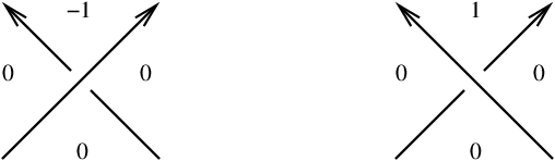
The filtration level of a state is the integer obtained by adding up the local contributions at each quadrant, which are determined by the crossing types of the knots, as indicated in Figure 2. The absolute grading of a state is determined by adding up another local contribution, pictured in Figure 3.

We have the following result from [18]:
Theorem 2.3.
Fix a generic knot projection for a knot . There is a one-to-one correspondence with generators of and states whose associated filtration level is . Under this correspondence, the absolute grading of a state in the above sense coincides with the absolute degree of the corresponding generator of .
Definition 2.4.
Fix a decorated knot projection. An essential interval is a sequence of consecutive edges with the following properties:
- •
the distinguished edge appears in the sequence, so we can write
where here , and is the successor of for all ,
- •
the immersed arcs
and are pairwise disjoint
- •
as we traverse the arc according to the orientation of , i.e. starting at the vertex , and then passing through in order, all of the crossings we encounter for the first time have the same type (i.e. they are all either over- or under-crossings); similarly, as we traverse the arc backwards, i.e. starting at , and proceeding through till , all the crossings we encounter the first time have the same type (which might be different different from the crossing type encountered along ).
Definition 2.5.
Fix a decorated knot projection, and also an essential interval . Each edge inherits an orientation from , and we write its endpoints as , so that are the vertices in the order they appear along . An -essential state is a state with the following properties:
- •
for , if , then the corner containing contains the edge on its boundary
- •
for , if , then the corner containing contains the edge on its boundary.
Proposition 2.6.
Proof. Recall that the Heegaard surface constructed in [18] is obtained as a boundary regular neighborhood of the knot projection. For each vertex , we have a -curve denoted , and at the distinguished , we choose a meridian for the knot which is supported near . Then, on either side of that meridian in the Heegaard surface, we choose a pair of basepoints and for the definition of .
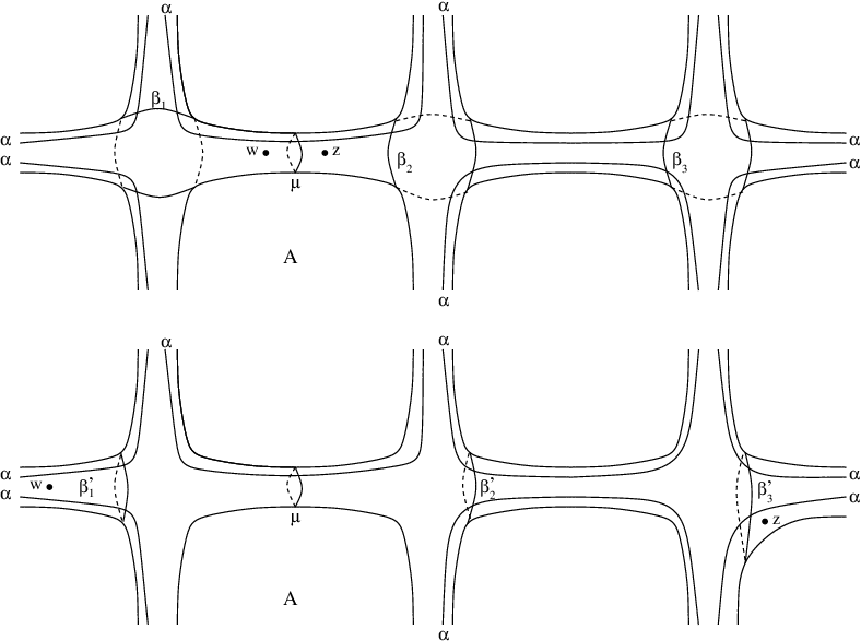
Suppose for simplicity that all the are distinct (i.e. that is an embedded arc in ). To simplify the Heegaard diagram as above, we move the two basepoints further away from the meridian, so that we can handleslide the -curves belonging to and across , to get new curves and . We continue handlesliding in this manner – across and across – until we have a new sequence of -curves which now meet always at most two -curves (rather than four). The hypothesis on the crossing types was used to ensure that the reference points could always be moved out of the handlesliding region (without crossing any of the attaching circles). This procedure is illustrated in Figure 4. It is not difficult to modify the above procedure when and have self-intersections.
Of course, the notion of essential arc, and the above proposition depends on the choice of essential interval. However, for some decorated knot projections, there is always a unique maximal essential interval. Indeed, this is the case for all the projections we consider in this paper, and hence, with this understood, we call a state an essential state if it is -essential for this maximal essential interval .
2.2. The combinatorics of domains, and the multi-filtration
Of course, the calculation of requires an explicit understanding of the differential in the complex , which in turn involves a pseudo-holomorphic curve count. More precisely, given a pair of states and (whose filtration level coincides, and whose absolute gradings differ by one), letting and denote the corresponding generators of , there is a unique homotopy class of Whitney disk with . The component of is the signed count of points in the moduli space of pseudo-holomorphic representatives of (modulo translation). At present, this count does not have a direct combinatorial description. However, there are combinatorial conditions on and which ensure that it vanishes.
Let be a graph for the knot projection of with edges. We order the edges of , so that is the marked edge, and the others appear in the order in which they are encountered by moving along (with its specified orientation). Let denote the vertex at the intersection of with (note that each vertex in appears as for two different values of , once as an overcrossing, and once as an undercrossing). We can associate to each state a multi-filtration-level
as follows:
Definition 2.7.
Fix a decorated knot projection. We define a partial ordering on the set of states, as follows: if and are two different states, then if for all edges , is a pair of non-negative integers.
An example of two states and for which and is illustrated in Figure 5.
Proposition 2.8.
Suppose that and represent the same filtration level, and indeed suppose that appears in with non-zero multiplicity, then .
Proof. Let denote the Heegaard diagram for used for Theorem 2.3. Consider an edge in the knot projection which does not meet the one of the two distinguished regions in the knot diagram. This edge, then, gives rise to a cylinder in the Heegaard diagram, which is divided into two squares by the -arcs. We place one reference point in the “top” part of the diagram, and another one in the “bottom” part. It is easy to see (after a straightforward case-by-case analysis of and ) that if is the homotopy class with , then
The result now follows from the basic fact that if has a pseudo-holomorphic representative (for suitably small perturbations of the holomorphic condition), then all these multiplicities must be non-negative (c.f. Lemma of [13]).
Note that the above argument also applies when the Heegaard diagram is “simplified” as in Proposition 2.6, only in that case, one uses the mult-filtration only over those edges which are not in the essential interval.

2.3. Trees
States admit a rather economical description in graph-theoretic terms (see also [6]). The regions in the complement of the planar projection can be colored black and white in a chessboard pattern, by the rule that any two regions which share an edge have opposite color. There is then an associated “black graph”, whose vertices correspond to the regions colored black, and whose edges correspond to vertices in , which connect the opposite black regions. We let (resp. ) denote the black (resp. white) region whose boundary contains the distinguished edge .
In these terms, states are in one-to-one correspondence with the maximal subtrees of the black graph. Given a state , we associate to it the union of vertices of , thought of now as edges in the black graph, to which associates a black quadrant. This gives the maximal black subtree associated to the state .
Conversely, given a black subtree , we can orient the edges so that the “root” is the distinguished black region , and all edges point away from this root. We construct the black part of the corresponding vertex assignment, as follows. Let be a vertex of which corresponds to some edge of . With respect to the induced orientation on , this oriented edge of points to a uniquely determined endpoint , which in turn corresponds to one of the two black quadrants (in ) which meet at . We let , then, be the quadrant corresponding to . To determine the rest of the vertex assignment, we first consider the dual white graph , obtained from the white graph by deleting all the edges corresponding to the vertices appearing in the black subtree . Note that is actually a tree, and repeat the above procedure, now for the white quadrants.
Clearly, one can reformulate the results of Theorem 2.3 in terms of these graphs. Each edge of both the black and white graphs inherits a label among the numbers : an edge in the white (resp. black) graph is labelled with if the two white (resp. black) quadrants meeting at the corresponding vertex both are have grading contribution (c.f. Figure 3), and it is labelled with if one of the two white (resp. black) graph is labelled with . We call edges labelled with neutral edges, and view them as unoriented, while the non-neutral ones are oriented (so as to point away from the vertex corresponding to the quadrant labelled with in Figure 3).
Given a black tree , let be its dual white tree, and orient both as before (so that the edges of and point away from and respectively). Then, twice the filtration level corresponding to is obtained as follows. We sum over all edges in the label of the edge in times if its orientation as an edge of the black graph agrees with the the induced orientation coming from , and if the orientations disagree (note here that this last sign is irrelevant for neutral edges); and then add to that the corresponding sum for all edges of the dual white graph .
Similarly, the grading level corresponding to is obtained by summing over all edges in the label of the edge in , provided that its orientation agrees with the induced orientation coming from (and zero otherwise), and once again adding the corresponding sum for .
2.4. Exact Sequences
In a different direction, we derived in [16] a “skein exact sequence”, which we recall here.
Suppose that is an oriented knot in , and we have a disk which meets in two algebraically cancelling points. If we perform surgery on , we obtain a new knot in , which is obtained from by introducing a full twist in a tubular neighborhood along . Performing surgery on gives us another knot with a full twist introduced in the other direction. There is a third link which is obtained by resolving the knot (so as to miss entirely). Recall [16] that the link invariant in this case is, by definition, the knot invariant for the knot in obtained by performing a zero-surgery along .
In [16], we established skein exact sequences for each integer
and
where the maps and are induced by two-handle additions.
It will be useful to us to have the following compatibility result about and :
Lemma 2.9.
For the above two exact sequences, the composite
is trivial.
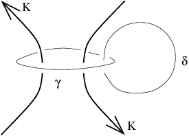
Proof. The map is induced by cobordism formed by zero-surgery on , while is induced by the cobordism formed by zero-surgery on another unknot which links once (and does not link the knot ). As in [14], we obtain the same map if we switch the order in which we perform the two two-handle additions: first we perform zero-surgery on , and then zero-surgery on (see Figure 6). However, in this latter ordering, we factor through the three-manifold (and the knot is contained entirely in the summand. It is easy to adapt the Künneth principle for connected sums in this context (see especially Proposition of [12]) to see that
| (5) |
Of course, , but our reason for writing the answer in this form is that we have now an action of on (induced from the corresponding action on ). The above isomorphism is compatible with this action of (where acts on the right-hand-side through its natural action on , c.f. Section of [13]). Now, maps to the kernel of the -action, since the curve representing is null-homologous in the four-manifold obtained by attaching a two-handle along to ; while is trivial on the image of the -action because, once again, is null-homologous in the corresponding four-manifold (compare [14]). But in the description of the -action from Equation (5), it is clear that the image of coincides with the kernel of , completing the proof.
3. Calculations for the Kinoshita-Terasaka knots
Consider the Kinoshita-Terasaka knots with . All the knots have trivial Alexander polynomial, but the knots themselves are non-trivial when and . Indeed, Gabai exhibits a Seifert surface for of genus and proves (c.f. [4]) that this Seifert surface has minimal genus.
We shall focus first on the case where . We distinguish the edge connecting the base of the and strands opposite to where the () twisting takes place – this is indicated by the point pictured in Figure 1. We have illustrated the “black graph” of , in Figure 7. For the black graph, there are two edges, labeled and , and four chains , , and . The edges , , , and are labeled with , while those of type and are labeled with . The distinguished black region corresponds to the vertex where , , , and meet. The vertices of the white graph are, of course, the regions in the complement of this planar graph. The region bounded by the chain of and and the edge corresponds to the distinguished white region. In fact, since none of the black edges is neutral, all of the white ones are.

We calculate in the case where using Theorem 2.3, together with the multi-filtration (Proposition 2.8). The case where is arbitrary will follow from properties of the skein exact sequence c.f. Lemma 2.9 (though one could alternately give a more direct argument using the multi-filtrations).
Proof of Theorem 1.1 when . It is easy to see that there are two trees and which represent filtration level : the tree does not contain , , , or , while the tree does not contain , , , or . These trees are illustrated in Figure 8.


Moreover, the grading of is given by , while the grading of is given by . It is straightforward to verify that for the multifiltration (see Figure 9 for an illustration) and hence, according to Proposition 2.8, . These calculations show that
Note that this is equivalent to the statement of the theorem (with ), in view of the symmetry of the knot Floer homology groups (c.f. Equation (2)).
Calculation for an pretzel link. Note that there is a skein exact sequences of the form
| (6) |
where is an oriented pretzel link which is independent of . (Strictly speaking, the notation for and ought to include the level , but we suppress this for readibility.) The maps and both decrease absolute grading by . In fact, according to Lemma 2.9,
| (7) |
Moreover, is the unknot. Specializing to the case where , and it follows at once that
| (8) |
and the map is an isomorphism.
Proof of Theorem 1.1 for arbitrary . To establish the theorem for all we prove inductively both the theorem, and also the statement that the map is injective. The basic case was established above. For the inductive step, if is not injective, then would have to be non-trivial, but this contradicts the injectivity of (which holds by the inductive hypothesis), together with Lemma 2.9, in the form of Equation (7). ∎
3.1. Additional remarks
Consider the case of with . By moving the marked edge, we obtain various chain complexes representing . Typically, subtrees which represent filtration level vary as we move the marked edge. However, since the white graph consists of neutral edges only, if we choose our marked edge so that the distinguished black region remains unchanged – there are four possible choices – then the maps from maximal subtrees to filtration levels and degrees are unchanged. However, the map from maximal subtrees to states, of course, varies, and more interestingly, the induced partial ordering on subtrees can change, too. For example, if we mark the edge of opposite to the edge containing (c.f. Figure 1), then it is easy to see that the two generators and described in the proof of Theorem 1.1 are still the two representatives for filtration level , and their dimensions are and . However, with this choice of marked edge, it is now the case that .
4. Calculations for the Conway knots
We consider the Conway mutants of the Kinoshita-Terasaka knots. The calculation of proceeds similarly to the calculations from Section 3. Note that the knot can be given the eleven-crossing presentation pictured in Figure 5. In this case, if we place the reference point where the arrow is indicated, and use the simplification of the Heegaard diagram described in Section 2, then it is straightforward to see that in filtration level there are only two inessential states, the two states and pictured in the figure, and they have absolute grading and respectively. However, , since , as illustrated in the figure, verifying Theorem 1.2 for , .
As before, we begin by restricting to the case where . Rather than drawing the black graph in this case, we indicate the necessary modifications to Figure 7. (Note that it is not hard to find projections with fewer essential states than the ones we describe – indeed, in the desired filtration level, we can arrange for there to be only two essential states, as in the case with considered above. However the diagrams we describe presently have the advantage that they are easier to describe in words.) The black graph of looks just like that for , except that now there are edges of type , and only edges of type . Moreover, the edges labeled with are , , and , and the edges labeled with are and . In particular all edges in the dual white graph remain neutral. We choose our marked edge to contain the point in Figure 1 (after mutating). Correspondingly, now, the distinguished black edge at the vertex between and , and the distinguished white region is bounded by the chains , and the edge .
Lemma 4.1.
For the diagram of described here with , there are Kauffman states representing filtration level . Of these, are in dimension , which we denote , , , and , and are in dimension , which we denote , , and . (Note that these states are explicitly identified in the proof below, which also explains their notation. See also Figure 10.) In the case where , we have only essential states: the two states and are missing from this diagram.

Proof. Notice that there are a total of edges in the black graph, and in fact a maximal spanning tree must contain exactly edges. It is clear that a maximal tree which contains neither nor has filtration level at most .
Thus, all maximal subtrees with filtration level contain either or . Now, if is a maximal subtree which contains one of or , then clearly, it must contain at least one of the chains , , or . Indeed, it cannot contain more than one. Accordingly, we say that a tree is of type if it contains the chain and the vertex . We analyze the eight cases separately.
Trees of type which represent filtration level , we claim, cannot contain the edge . But a tree which contains , and does not contain corresponds to an inessential vertex assignment – and indeed, in the case where , such trees never represent filtration level . The same remarks rule out trees of type , and similar remarks rule out trees of type , and .
It is easy to see that there is only one tree of type which represents filtration level , and it is the one which does not contain , , , and . Similarly, there is only one tree of type , and it does not contain , , , and .
Assume for the moment that . There are three trees of type representing filtration level : one which does not contain , , , and , which we denote , one which does not contain , , , and , which we denote , and one which does not contain , , , and . Similarly, there are three trees of type representing filtration level , which we denote , where is gotten from by deleting and and adding and . The case where works similarly, except that the states and do not exist.
Lemma 4.2.
Consider the essential generators listed in Lemma 4.1 for with . These have the following ordering properties for the multi-filtration:
| (9) |
and
| (10) |
Moreover, fixing fix , and letting be the homotopy class with , we have that
| (11) |
The same holds for the corresponding homotopy class in . When , the same remarks hold, excluding states and .
Proof. Verifying the order properties is straightforward. Some of the work in verifying Relation (10) is shortened, given Relation (9), and the observation that the difference in the multi-filtering between and for is supported in a single edge; a similar remark holds for and . For the statement about homotopy classes, observe that all of these homotopy classes are represented by quadrilaterals, and hence can be calculated by one-variable complex analysis (compare Section of [12]).
Proof of Theorem 1.2. Again, we start with the case where . We use the complex described in Lemma 4.1.
According to Lemma 4.2 (c.f. Relations 9) together with the basic property of the multi-filtration (Proposition 2.8), the chain complex admits a subcomplex generated by and . Indeed, the homology of this complex is trivial, in view of Equation (11). Thus, is calculated as the homology of the induced quotient complex. Another application of this principle allows us to cancel also the generators and . The leftover complex, generated by , , , and , now admits a quotient complex which is generated by and and hence, according to Equation (11), has trivial homology. (Note that this step is skipped when .)
Thus, is calculated by the homology of the remaining complex generated by and . Since , it follows that the homology is
verifying the calculation of when .
Note that for the pictured knot projection, are two states representing filtration level (and none representing higher filtration levels). However, these two states are quickly seen to cancel (they, too, are connected by a quadrilateral).
To go from to arbitrary , observe that is an unknot. Thus, we have a skein exact sequence relating the various Conway knots, corresponding to Equation (12):
| (12) |
for any integer , where now is an oriented pretzel link, rather than the pretzel link belonging to the Kinoshita-Terasaka knots considered earlier. (Of course, is a mutant of , and both have trivial Alexander polynomial.)
With these remarks in place, the induction used to verify the theorem runs exactly as it did in the case of . As a consequence, we also obtain the following formula for :
∎
4.1. A Seifert surface
Note that the Conway knot has a genus Seifert surface, obtained by a straightforward modification of the picture for the case where , described in [3].
We describe first the Seifert surface for the pretzel link. We “pull down” the overcrossing which connects the first two tassles and the undercrossing which connects the second two. And then, we consider the black regions for the knot projection. Those in turn we label with signs, with the rule that no two regions which meet at a vertex have the same sign. The Seifert surface for this pretzel link is obtained by connecting these black regions by half-twists at each vertex. It is easy to see that the surface obtained in this manner is orientable, and has . We have illustrated this data in Figure 11 for the case where .

We can plumb this with a cylinder with full twists in it (i.e. forming a Murasugi sum), to obtain a Seifert surface for the Conway knot whose genus is .
5. Calculations for the pretzel knots
In this section, we consider the family of pretzel knots , where , and are odd. We follow the usual conventions from knot theory here (c.f. [10]) for the direction of the twisting (which, unfortunately, seems to be opposite from the convention used in [17]), compare Figure 12.

There are some relations amongst the pretzel knots. For example, it is easy to see that , and that is the unknot, for any .
Recall that
thus, there are infinitely many examples with trivial Alexander polynomial. When , , and are all positive, then the signature of is given by
When is an even integer, denote the torus link, oriented so that the two strands – which we can think of as supported inside a solid torus – are oriented so that the algebraic intersection of with a disk transverse to the solid torus is zero. In this case,
Moreover, the signature of is , depending on the sign of :
Clearly, if we resolve one of the intersection points corresponding to the first strand in , we obtain the torus link . Thus, the skein long exact sequence of [16] in this case gives
| (13) |
where here and preserve filtration levels, and both drop absolute grading by . The map also preserves filtration level, and it preserves the parity of absolute grading.
When , , and all have the same sign, then the usual projection of is alternating. In this case, the knot Floer homology is determined by [18]. Specifically, in [18], it is shown that if is a non-split, oriented, alternating link with signature , and Alexander-Conway polynomial , then if we write
then
| (14) |
Thus, by reflecting knot if necessary, we are left with the case where and . Note that when , is a non-split, alternating link.
Proposition 5.1.
Consider the pretzel knot with . Then, if , we have that
Proof. For fixed , we prove the result by induction on both and .
Consider the base case where . Using the skein exact sequence in the form of Equation (13) with , and the relation that is the unknot, we see at once that
Moreover, since is alternating, Theorem of [18] applies, and hence, in this case Equation (14) specializes to give
For the inductive step on , suppose we know the result for , and suppose that and . The condition that ensures that still has signature , and hence is supported in dimension ; by the inductive hypothesis, is supported in dimension . Thus, the skein exact sequence forces to be supported in dimension one. The inductive step on works analogously.
We now turn to the case where .
Lemma 5.2.
Let be the pretzel knot with and . Then,
Proof. This is proven by induction on and , starting with the basic case where . Suppose for concreteness that . Then, it is easy to see that is independent of : the middle term in the skein exact sequence (Equation (13)) vanishes: it corresponds to of the two-component unlink, whose knot Floer homology is supported in filtration level zero. Thus, it can be calculated in the case where , so Proposition 5.1 applies, proving that is supported entirely in dimension one, where its rank is precisely .
For the inductive step, suppose we are increasing by one, and apply Equation (13). Now, the middle term has signature , and hence is supported in dimension . In particular, the map
is surjective, providing the inductive step for increasing . Increasing follows similarly.
To proceed, we use a decorated knot projection for , and consider the multi-filtration on states from Section 2.
Specifically, choose a knot projection for whose corresponding black graph consists of two vertices with degree three, connected by three linear strands of edges , , and . The vertex meeting the edges , , and is the distinguished black vertex. The corresponding distinguished black region is a triangle with three edges , , and , with facing the vertex corresponding to , facing from , and facing . Our distinguished edge for the decorated knot projection is .
Let resp. , resp. be the Kauffman state corresponding to the tree which is obtained by deleting and resp. and resp. and from the black graph.

Lemma 5.3.
For the pretzel knot with , the generators of in dimension one are
and the generators in dimension two are of the form
There are no other generators of .
Proof. This follows at once from the above diagram.
Lemma 5.4.
For the marked edges and , we have that
Proof. This, too, follows quickly from the diagram.
Lemma 5.5.
For the pretzel knot with , we have that .
Proof. According to Lemma 5.4 (together with Proposition 2.8), the generators (where and ) with , of which there are , all lie in the cokernel of the boundary operator. Similarly, the generators (where and ) with , of which there are another , all lie in the cokernel of the boundary operator. Since there are no generators in dimension zero (according to Lemma 5.3), the stated bound follows.
Proof of Theorem 1.3. The case where is established in Proposition 5.1. Together, Lemmas 5.2 and 5.5 show that . The rest of the theorem now follows at once from Lemma 5.3. ∎
Proposition 5.6.
Let be a knot with . Then, if
| and |
then no integral surgery of along is a Seifert fibered space.
Proof. By reflecting the knot if necessary, we can assume that is Seifert fibered for some .
As in the proof of Lemma of [19], Section of [16] gives a -submodule of (for sufficiently large ) which is isomorphic to ; indeed, we have a short exact sequence:
The above is a map of -modules, and the action on is trivial. It follows now that
Considering the integer surgeries long exact sequence, it follows that for all
In view of our hypotheses, then is non-trivial in both even and odd degrees. On the other hand, results from [20] show that for a Seifert fibered space with , is supported in either even or odd degrees (this is proved in Corollary of [20]).
6. Knots with few crossings
We give here another application of the results of Proposition 2.6, showing that the Floer homology groups of all but two of the knots with nine or fewer crossings behave like the Floer homology of alternating knots. The two counterexamples to this are the -torus knot (which appears in the tables under the name ) and a certain nine-crossing knot . In fact, the knot Floer homologies of these two knots have been determined in Theorem of [15] and Proposition of [16] respectively, where it is shown that:
(Note that the standard knot tables do not distinguish a knot from its mirror. For the above statements, we have chosen the versions of the knots whose signature is negative.)
Theorem 6.1.
Except for the knots and , any other knot admitting a projection with nine or fewer crossings has the property that
| (17) |
where here denotes the signature of the knot , and the are the coefficients of its symmetrized Alexander polynomial.
Proof. Of course, for alternating knots, the theorem follows from [18]. Now, there there are only nine non-alternating knots to consider here according to standard knot tables, see for example [1]. One of these, the knot , which is the pretzel knot , will be handled separately. We illustrate distinguished edges for knot projections for the remaining eight knots in Figure 14 (but dropping orientations).

Now, of these eight, we consider separately as well. For the remaining seven knots, it is straightforward to see that in each filtration level, all of the essential states have the same absolute grading. Indeed, calculating these absolute gradings, one can readily verify that for these knots, the essential states with filtration level all have absolute grading . In view of Proposition 2.6, the theorem then follows for these seven knots.
For the case of , a direct analysis using the illustrated decorated knot projection verifies Equation (17) for all , and hence also for all , in view of the symmetry of , Equation (2). In the case where , now, we claim that there are three generators, one in dimension , and two in dimension . In fact, a closer look at the states reveals that the essential state in dimension can be connected to an essential state in dimension by a homotopy class whose associated domain is an octagon (with multiplicity , missing the reference point ). Compare with the genus four Heegaard diagram of pictured in Figure 16, where there are three generators for , , with homotopy classes connecting resp. to represented by octagons. It now follows easily that for a homotopy class whose domain is an octagon,
Hence, we have that the boundary operator in is non-trivial, and indeed that the homology in filtration level is given by , completing the verification of Equation (17) for .


References
- [1] G. Burde and H. Zieschang. Knots. Number 5 in de Gruyter Studies in Mathematics. Walter de Gruyter & Co., 1985.
- [2] E. Eftekhary. Heegaard floer homologies of pretzel knots. math.GT/0311419.
- [3] D. Gabai. Foliations and genera of links. Topology, 23(4):381–394, 1984.
- [4] D. Gabai. Genera of the arborescent links., volume 59, pages i–viii and 1–98. Amer. Math. Soc., 1986.
- [5] H. Goda and M. Teragaito. Dehn surgeries on knots which yield lens spaces and genera of knots. Math. Proc. Cambridge Philos. Soc., 129(3):501–515, 2000.
- [6] L. H. Kauffman. Formal knot theory. Number 30 in Mathematical Notes. Princeton University Press, 1983.
- [7] M. Khovanov. A categorification of the Jones polynomial. Duke Math. J., 101(3):359–426, 2000.
- [8] S. Kinoshita and H. Terasaka. On unions of knots. Osaka Math. J., 9:131–153, 1957.
- [9] P. B. Kronheimer and T. S. Mrowka. Scalar curvature and the Thurston norm. Math. Res. Lett., 4(6):931–937, 1997.
- [10] W. B. R. Lickorish. An introduction to knot theory, volume 175 of Graduate Texts in Mathematics. Springer-Verlag, 1997.
- [11] T. W. Mattman. The Culler-Shalen seminorms of the pretzel knot. math.GT/9911085, 1999.
- [12] P. S. Ozsváth and Z. Szabó. Holomorphic disks and three-manifold invariants: properties and applications. math.SG/0105202.
- [13] P. S. Ozsváth and Z. Szabó. Holomorphic disks and topological invariants for closed three-manifolds. math.SG/0101206.
- [14] P. S. Ozsváth and Z. Szabó. Holomorphic triangles and invariants for smooth four-manifolds. math.SG/0110169.
- [15] P. S. Ozsváth and Z. Szabó. On knot Floer homology and lens space surgeries. math.GT/0303017.
- [16] P. S. Ozsváth and Z. Szabó. Holomorphic disks and knot invariants. math.GT/0209056, 2002.
- [17] P. S. Ozsváth and Z. Szabó. Absolutely graded Floer homologies and intersection forms for four-manifolds with boundary. Adv. Math., 173(2):179–261, 2003.
- [18] P. S. Ozsváth and Z. Szabó. Heegaard Floer homology and alternating knots. Geom. Topol., 7:225–254 (electronic), 2003.
- [19] P. S. Ozsváth and Z. Szabó. On Heegaard Floer homology and Seifert fibered surgeries. math.SG/0301026, 2003.
- [20] P. S. Ozsváth and Z. Szabó. On the Floer homology of plumbed three-manifolds. Geometry and Topology, 7:185–224, 2003.
- [21] J. Rasmussen. Floer homology of surgeries on two-bridge knots. Algebr. Geom. Topol., 2:757–789 (electronic), 2002.
- [22] J. Rasmussen. Floer homology and knot complements. PhD thesis, Harvard University, 2003. math.GT/0306378.
- [23] S. M. Wehrli. Khovanov homology and Conway mutation. math.GT/0301312, 2003.