Supercritical multitype branching processes:
the ancestral types of typical individuals

Looking at the time evolution of a population one has two possible perspectives: either forward or backward in time. In the first case one observes the characteristics of the population at a given time $t$ and asks for its behaviour as $t$ increases to infinity. A classical model that describes the unrestricted reproduction of independent individuals is the (multitype) branching process, and a principal result in the supercritical case is the Kesten-Stigum theorem [16], which describes the population size and relative frequencies of types; see Theorem 1 for the precise statement. A different situation arises if the population size is kept constant; this leads to certain interacting particle systems, like the Moran model and its relatives (for review, see [7]). By way of contrast, the backwards – or retrospective – aspect of the population concerns the lineages extending back into the past from the presently living individuals and asks for the characteristics of the ancestors along such lineages. One famous example is Kingman’s coalescent (see [17, 18], and [22] for a review), the backward version of the Moran model. As was observed e.g. by Jagers [14] and Jagers and Nerman [15], it is also rewarding to study the backward aspects of multitype branching processes; this point of view has turned out as crucial in recent biological applications [11]. It is the aim of this article to pursue this last line of research further. We do so in continuous time because this gives us the opportunity to transfer some powerful methods recently developed for discrete time. We also concentrate on the supercritical case.

Specifically, we consider the individuals alive at some time $t$ and investigate the types of their ancestors at an earlier time, $t-u$. We will show the following.

• •

  When $t$ resp. $t$ and $u$ tend to infinity, both time average and population average of ancestral types converge to a particular distribution $\alpha$ almost surely on non-extinction (Theorems 2 and 4).

This $\alpha$ will be called the ancestral distribution of types; its components are $\alpha_{i}=\pi_{i}h_{i}$, where $\pi$ and $h$ are the (properly normalized) left and right Perron-Frobenius eigenvectors of the generator of the first-moment matrix.

More detailed information about the evolution of types along ancestral lineages is obtained through what we would like to call the retrospective mutation chain, a particular continuous-time Markov chain on the type space with $\alpha$ as its invariant distribution. We will show:

• •

  For all individuals alive at time $t$ up to an asymptotically negligible fraction, the time averaged empirical type evolution process tends in distribution to the stationary retrospective mutation chain, in the limit as $t\to\infty$, almost surely on non-extinction (Theorem 6).

One basic ingredient of our reasoning is a law of large numbers for population averages; see Proposition 11. A second crucial ingredient is a representation of the family tree in terms of a size-biased tree with trunk (with the retrospective mutation chain running along the trunk); see Theorem 8. This representation is the continuous-time analogue of the size-biased tree representation introduced by Lyons, Pemantle and Peres [20] and Kurtz, Lyons, Pemantle and Peres [19]. In passing, it allows us to extend their conceptual proof of the Kesten-Stigum theorem to continuous time. The third ingredient is the Donsker-Varadhan large deviation principle for the retrospective mutation chain [5, 6]. This implies a large deviation principle for the typical type evolution along the surviving lineages in the tree – see Theorem 14.

This paper is organized as follows. In the next section we recall the construction of the family tree for multitype branching processes in continuous time. Section 3 contains the precise statement of results. Section 4 is devoted to the size-biased tree with trunk, and the proofs of the main results are collected in Section 5.

We consider a continuous-time multitype branching process as described in Athreya and Ney [2, Ch. V.7]. To fix the notation we recall the basic setting here.

Let $S$ be a finite set of types. An individual of type $i\in S$ lives for an exponential time with parameter $a_{i}>0$, and then splits into a random offspring $N_{i}=(N_{ij})_{j\in S}$ with distribution $\mathsf{p}_{i}$ on $\mathbb{Z}^{S}_{+}$ and finite means $m_{ij}:=\mathbb{E}(N_{ij})$ for all $i,j\in S$; here, $N_{ij}$ is the number of $j$-children, and $\mathbb{Z}_{+}=\{0,1,\ldots\}$. We assume that the mean offspring matrix $\mathsf{M}=(m_{ij})_{i,j\in S}$ is irreducible.

According to Harris [10, Ch. VI], the associated random family tree can be constructed as follows. Let $\mathbb{X}=\bigcup_{n\geq 0}\mathbb{X}_{n}$, where $\mathbb{X}_{n}$ describes the virtual $n$’th generation. That is, $\mathbb{X}_{0}=S$, and $i_{0}\in\mathbb{X}_{0}$ specifies the type of the root, i.e., the founding ancestor. Next, $\mathbb{X}_{1}=S\times\mathbb{N}$, and the element $x=(i_{1},\ell_{1})\in\mathbb{X}_{1}$ is the $\ell_{1}$’th $i_{1}$-child of the root. Finally, for $n>1$, $\mathbb{X}_{n}=S^{n}\times\mathbb{N}^{n}$, and $x=(i_{1},\ldots,i_{n};\ell_{1},\ldots,\ell_{n})\in\mathbb{X}_{n}$ is the $\ell_{n}$-th $i_{n}$-child of its parent $\tilde{x}=(i_{1},\ldots,i_{n-1};\ell_{1},\ldots,\ell_{n-1})$; see Fig. 1. We write $\sigma(x)=i_{n}$ for the type of $x\in\mathbb{X}_{n}$. With each $x\in\mathbb{X}$ we associate

• •

  its random life time $\tau_{x}$, distributed exponentially with parameter $a_{\sigma(x)}$, and

• •

  its random offspring $N_{x}=(N_{x,j})_{j\in S}\in\mathbb{Z}_{+}^{S}$ with distribution $\mathsf{p}_{\sigma(x)}$

such that the family $\{\tau_{x},N_{x}:\,x\in\mathbb{X}\}$ is independent.

The random variables $N_{x}$ indicate which of the virtual individuals $x\in\mathbb{X}$ are actually realized, namely those in the random set $X=\bigcup_{n\geq 0}X_{n}$ defined recursively by

where $i_{0}$ is the prescribed type of the root. The random variables $\tau_{x}$ provide the proper time scale. Namely, for $x\in X$, let the splitting times $T_{x}$ be defined recursively by $T_{x}=T_{\tilde{x}}+\tau_{x}$ with $T_{\tilde{i_{0}}}:=0$. The lifetime interval of $x\in X$ is then $[T_{\tilde{x}},T_{x}\/\mathclose{[}$. Hence $X(t)=\{x\in X:\,T_{\tilde{x}}\leq t<T_{x}\}$ is the population at time $t$. One may visualize the resulting tree by identifying each $x\in X$ with an edge from $\tilde{x}$ to $x$ with length $\tau_{x}$ in the direction of time.

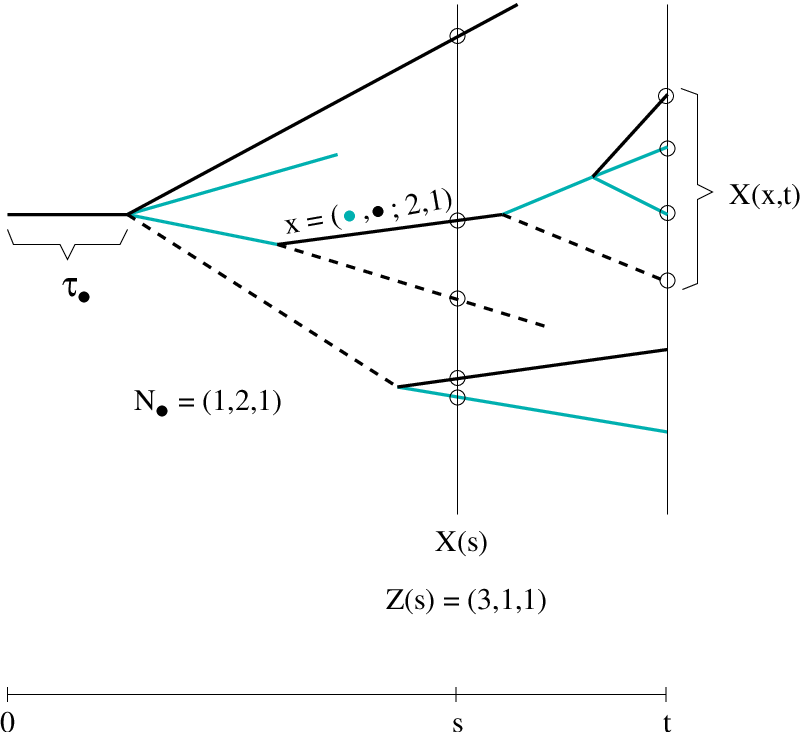
The family tree is completely determined by the process $X[0,\infty\/\mathclose{[}:=\big(X(t)\big)_{t\geq 0}$ which is a random element of $\Omega:=D\big([0,\infty\/\mathclose{[},\mathfrak{P}_{f}(\mathbb{X})\big)$, the Skorohod space of all càdlàg functions on $[0,\infty\/\mathclose{[}$ taking values in the (countable) set $\mathfrak{P}_{f}(\mathbb{X})$ of all finite subsets of $\mathbb{X}$. We write $\mathbb{P}^{i}$ for the distribution of $X[0,\infty\/\mathclose{[}$ on $\Omega$ when the type of the root is $i_{0}=i$, and $\mathbb{E}^{i}$ for the associated expectation. If $i_{0}$ is chosen randomly with distribution $\nu$, we write $\mathbb{P}^{\nu}$ and $\mathbb{E}^{\nu}$. We will often identify $X[0,\infty\/\mathclose{[}$ with the canonical process on $\Omega$.

For $0<s<t$ and $y\in X(t)$ we write $y(s)$ for its unique ancestor living at time $s$. On the other hand, for $x\in X(s)$ we let

denote the set of descendants of $x$ living at time $t$; cf. Fig. 1. In the above, the concatenation $xy$ of two strings $x,y\in\mathbb{X}$ is defined in the obvious way, and the empty string is considered as an ancestor of type $\sigma(x)$; i.e., $X(x,t)=\{\sigma(x)\}$ as long as $x\in X(t)$. By the loss-of-memory property of the exponential distributions, the descendant trees $X(x,[s,\infty\/\mathclose{[})=(X(x,t))_{t\geq s}$ with $x\in X(s)$ are conditionally independent given $X[0,s]$, with distribution $\mathbb{P}^{\sigma(x)}$. We will also consider the counting measures

on $S$, where $\delta_{i}$ is the Dirac measure at $i$. $Z(t)$ and $Z(x,t)$ count the type frequencies in the population $X(t)$ resp. the subpopulation $X(x,t)$ of $x$-descendants. In particular, $Z_{j}(t)$ is the cardinality of $X_{j}(t)=\{x\in X(t):\sigma(x)=j\}$, the subpopulation of type $j\in S$, and $\|Z(t)\|:=\sum_{j\in S}Z_{j}(t)=|X(t)|$ is the total size of the population.

It is well-known (cf. [2], p. 202, Eq. 9) that $\mathbb{E}^{i}(Z_{j}(t))=(e^{t\mathsf{A}})_{ij}$ for all $i,j\in S$, where the generator matrix $\mathsf{A}=(a_{ij})_{i,j\in S}$ is given by

By the irreducibility of $\mathsf{M}$, $\mathsf{A}$ is also irreducible, so that the first moment matrix $(\mathbb{E}^{i}(Z_{j}(t)))_{i,j\in S}$ has positive entries for any $t>0$. (This property is often called ‘positive regularity’, see [2, p. 202].) Perron-Frobenius theory then tells us that the matrix $\mathsf{A}$ has a principal eigenvalue $\lambda$ (i.e., a real eigenvalue exceeding the real parts of all other eigenvalues), and associated positive left and right eigenvectors $\pi$ and $h$ which will be normalized s.t. $\langle\pi,\mathsf{1}\rangle=1=\langle\pi,h\rangle$. Here we think of the row vector $\pi$ as a probability measure, of the column vectors $h$ and $\mathsf{1}=(1,\ldots,1)^{T}$ as functions on $S$, and of the scalar product $\langle\pi,h\rangle=\sum_{i}\pi_{i}h_{i}$ as the associated expectation. We are mainly interested in the supercritical case $\lambda>0$. In this case we write

for the event that the population survives for all times.

It is a remarkable fact that the almost-sure behaviour of the family tree is, to a large extent, already determined by the the global quantities $\lambda,\pi,h$. One prominent example is the following continuous-time version of the Kesten-Stigum theorem (see [16] for the discrete-time original, [1] for the continuous-time version, and [19] for the recent discrete-time conceptual proof).

For the sake of reference we provide here a full proof extending the conceptual discrete-time proof of [19] to our continuous-time setting. Assertion (a) reveals that the left eigenvector $\pi$ holds the asymptotic proportions of the types in the population, and statement (b) implies that

is the almost sure exponential growth rate of the population in the case of survival. In fact, this statement does not require condition (2.4); see the proof of Theorem 6 in Section 5.3. The $i$-th coordinate $h_{i}$ of the right eigenvector $h$ measures the long-term fertility of an $i$-individual. In fact, $h_{i}$ is also characterized by the limiting relation

cf. Remark 9(a) below.

We still consider the supercritical case $\lambda>0$. We are interested in the mutation behaviour of the population tree. More specifically, we ask for the behaviour of the sequence of types along a typical branch of this tree. It turns out that this behaviour is again completely determined by the global quantities $\lambda,\pi,h$. A key role is played by the probability vector $\alpha=(\alpha_{i})_{i\in S}$ with components $\alpha_{i}=\pi_{i}h_{i}$. As observed by Jagers [14, Corollary 1], Jagers and Nerman [15, Prop. 1], and Hermisson et al. [11], this probability vector describes the distribution of ancestral types of an equilibrium population with type frequencies given by $\pi$. The vector $\alpha$ will therefore be called the ancestral distribution. Our results below shed some additional light on the significance of $\alpha$.

To begin, we consider a typical individual $x\in X(t)$ alive at some large time $t$ and ask for the type $\sigma(x(t{-}u))$ of its ancestor $x(t{-}u)$ living at some earlier time $t{-}u$. We find that $\sigma(x(t{-}u))$ is asymptotically distributed according to $\alpha$. Specifically, let $0<u<t$ and

be the empirical ancestral type distribution at time $t{-}u$ taken over the population $X(t)$. (Of course, this definition requires that $X(t)\neq\varnothing$.)

The proof will be given in Section 5.2. We would like to remark that a slightly weaker result under slightly stronger conditions (convergence in probability under assumption (2.4)) follows immediately from Corollary 4 of Jagers and Nerman [15], where very general population averages are considered.

In our next theorem we ask for the time average of types along the line of descent leading to a typical $x\in X(t)$. This time average is given by the empirical distribution

of the process $\sigma(x[0,t])=\big(\sigma(x(s))\big)_{0\leq s\leq t}$. Note that ${L}^{x}(t)$ belongs to the simplex $\mathcal{P}(S)$ of all probability vectors on $S$; $\mathcal{P}(S)$ will be equipped with the usual total variation distance $\|\cdot\|$. To describe the behaviour of ${L}^{x}(t)$ for a typical $x\in X(t)$ we have to step one level higher and to consider the empirical distribution of ${L}^{x}(t)$ taken over the population $x\in X(t)$. This empirical distribution belongs to $\mathcal{P}(\mathcal{P}(S))$, the set of probability measures on $\mathcal{P}(S)$, which will be equipped with the weak topology.

Theorem 4 is in fact a corollary of our next theorem which considers the complete mutation history along a typical line of descent. To state this result we need some preparations. We introduce first the mutation process on $S$ which will turn out to describe the time-averaged mutation behaviour along an ancestral line.

We note that $\mathsf{G}$ is indeed a generator because $a_{i}\sum_{j\in S}m_{ij}h_{j}=\sum_{j\in S}(a_{i}\delta_{ij}+a_{ij})h_{j}=(a_{i}{+}\lambda)h_{i}$ by (2.3). Since $\mathsf{M}$ is irreducible by assumption, $\mathsf{G}$ is irreducible as well. It is also immediate that the ancestral distribution $\alpha$ is the (unique) stationary distribution of $\mathsf{G}$. The retrospective mutation chain was identified by Jagers [13, p. 195] and may be interpreted as the forward version of the backward Markov chain [15, Proposition 1] that results from picking individuals randomly from the stationary type distribution $\pi$ and following their lines of descent backward in time. This gives the transition rates

which corresponds to the time reversal of the retrospective mutation chain.

To set up the stage for Theorem 6 we let $\mathrm{\Sigma}=D(\mathbb{R},S)$ denote the space of all doubly infinite càdlàg paths in $S$. $\mathrm{\Sigma}$ will be equipped with the usual Skorohod topology which turns $\mathrm{\Sigma}$ into a Polish space; see e.g. [8], Section 3.5 and in particular Th. 5.6, for the case of the time interval $[0,\infty\/\mathclose{[}$. The associated Borel $\sigma$-algebra coincides with the $\sigma$-algebra generated by the evaluation maps $\mathrm{\Sigma}\ni\sigma\to\sigma(t)$, $t\in\mathbb{R}$ [8, p. 127, Prop. 7.1]. The time shift $\vartheta_{s}$ on $\mathrm{\Sigma}$ is defined by

We write $\mathcal{P}_{\Theta}(\mathrm{\Sigma})$ for the set of all probability measures on $\mathrm{\Sigma}$ which are invariant under the shift group $\Theta=(\vartheta_{s})_{s\in\mathbb{R}}$. Endowed with the weak topology, $\mathcal{P}_{\Theta}(\mathrm{\Sigma})$ is a Polish space [8, p. 101, Th. 1.7].

Next we introduce the time-averaged type evolution process of an individual in the population tree. For $t>0$ and $x\in X(t)$ we let $\sigma(x)_{t,\mathrm{per}}\in\mathrm{\Sigma}$ be defined by

where $s_{t}$ is the unique number in $[0,t\/\mathclose{[}$ with $s\equiv s_{t}\mod t$. That is, $\sigma(x)_{t,\mathrm{per}}\in\mathrm{\Sigma}$ is the periodically continued type history of $x$ up to time $t$. The time-averaged type evolution of $x$ is then described by the empirical type evolution process

We are interested in the typical behaviour of $R^{x}(t)$ when $x$ is picked at random from $X(t)$, the population at time $t$. This is captured in their empirical distribution, i.e., the population average

(As before, this definition requires that $X(t)\neq\varnothing$.) $\Gamma(t)$ is a random element of $\mathcal{P}(\mathcal{P}_{\Theta}(\mathrm{\Sigma}))$, the set of all probability measures on the Polish space $\mathcal{P}_{\Theta}(\mathrm{\Sigma})$, which is again equipped with the weak topology. In Section 5.3 we will prove:

In this section we construct a continuous-time version of the size-biased multitype Galton-Watson tree as introduced by Lyons, Pemantle, Peres, and Kurtz [20, 19]. Informally, this is a tree with a randomly selected trunk (or spine) along which time runs at a different rate and offspring is weighted according to its size; in particular, there is always at least one offspring along the trunk so that the trunk survives forever. The children off the trunk get ordinary (unbiased) descendant trees (the bushes). It will turn out that the trunk of the size-biased tree describes the evolution along a typical ancestral line that survives up to some fixed time. The construction is not confined to the supercritical case; that is, in this section $\lambda$ can have arbitrary sign.

First of all, for each type $i\in S$ we introduce the size-biased offspring distribution

where $\langle\kappa,h\rangle=\sum_{j}\kappa_{j}h_{j}$ and $c_{i}=1+\lambda/a_{i}$ is a normalizing constant. $\widehat{\mathsf{p}}_{i}$ will serve as the offspring distribution of an $i$-individual on the trunk; it is indeed a probability distribution since

by (2.3); note that $c_{i}$ is automatically positive. Next, when an $i$-individual on the trunk has offspring $\widehat{N}_{i}=(\widehat{N}_{ij})_{j\in S}$ with distribution $\widehat{\mathsf{p}}_{i}$, one of these offspring is chosen as the successor on the trunk, where children are picked with probability proportional to $h_{j}$ when their type is $j$. That is, the successor is of type $j$ with probability $\widehat{N}_{ij}\;h_{j}/\langle\widehat{N}_{i},h\rangle$ for a given offspring, and with probability

on average. These are precisely the jump probabilities of the retrospective mutation chain. Finally, the lifetime of an $i$-individual on the trunk will be exponential with parameter $a_{i}{+}\lambda$, which coincides again with the holding time parameter of the retrospective mutation chain. A corresponding embedded chain combined with size-biased waiting times also occurs when more general non-Markovian populations (i.e., with waiting times deviating from the exponential distribution) are traced backwards, see [15, Proposition 1].

We now construct the size-biased tree in detail. Let $\{\tau_{x},N_{x}:\,x\in\mathbb{X}\}$ be as in Section 2 and, independently of this, a sequence $\{\widehat{\tau}_{n},\widehat{N}_{n},\xi_{n}:n\geq 0\}$ of random variables with values in $\mathopen{]}\/0,\infty\/\mathclose{[}\,,\mathbb{Z}_{+}^{S},\mathbb{X}$ respectively such that, for a given type $i_{0}=i$ of the root, $\xi_{0}=i$ and

• •

  $\widehat{\tau}_{0},\widehat{N}_{0}$ are independent, $\widehat{\tau}_{0}$ has exponential distribution with parameter $a_{i}{+}\lambda$, $\widehat{N}_{0}$ has distribution $\widehat{\mathsf{p}}_{i}$, and $\xi_{1}$ has conditional distribution

  $$P\big(\xi_{1}=(i_{1},\ell_{1})|\widehat{N}_{0},\widehat{\tau}_{0}\big)=\frac{h_{i_{1}}}{\langle\widehat{N}_{0},h\rangle}\,I{\{\ell_{1}\leq\widehat{N}_{0,i_{1}}\}}$$

  for all $(i_{1},\ell_{1})\in\mathbb{X}_{1}$.

• •

  For any $n\geq 1$, conditionally on $\mathbb{F}_{n-1}=\sigma\{\widehat{\tau}_{k},\,\widehat{N}_{k},\,\xi_{k+1}:\,k<n\}$, $\widehat{\tau}_{n},\widehat{N}_{n}$ are independent and follow an exponential law with parameter $a_{\sigma(\xi_{n})}{+}\lambda$ resp. the law $\widehat{\mathsf{p}}_{\sigma(\xi_{n})}$, and

  $$P\big(\xi_{n+1}=(\xi_{n};i_{n+1},\ell_{n+1})|\mathbb{F}_{n-1},\widehat{\tau}_{n},\widehat{N}_{n}\big)=\frac{h_{i_{n+1}}}{\langle\widehat{N}_{n},h\rangle}I{\{\ell_{n+1}\leq\widehat{N}_{n,i_{n+1}}\}}$$

  for all $(i_{n+1},\ell_{n+1})\in S\times\mathbb{N}$, i.e., $\xi_{n+1}$ is a child of $\xi_{n}$ selected randomly with weight proportional to $h_{\sigma(\xi_{n+1})}$.

Define $\widehat{X}=\bigcup_{n\geq 0}\widehat{X}_{n}\subset\mathbb{X}$ recursively by $\widehat{X}_{0}=\{i\}$ and $\widehat{X}_{n}=\widehat{X}_{n}^{\sharp}\cup\widehat{X}_{n}^{\flat}$ with

the offspring of $\xi_{n-1}$, and

the offspring of all other individuals in $\widehat{X}_{n-1}$. (Note that in the last display there is no hat on $N$; that is, the bushes have unbiased offspring.) The split times $\widehat{T}_{x}$ are given by $\widehat{T}_{\xi_{0}}=\widehat{\tau}_{0}$, $\widehat{T}_{\xi_{n}}=\widehat{T}_{\xi_{n-1}}+\widehat{\tau}_{n}$ for $n\geq 1$, and $\widehat{T}_{x}=\widehat{T}_{\tilde{x}}+\tau_{x}$ if $x\in\widehat{X}\setminus\{\xi_{n}:\,n\geq 0\}$. (Again, in the latter case there is no hat on $\tau$, meaning that the individuals off the trunk have unbiased life times.) The total population at time $t$ is then given by

The selected trunk individual at time $t$ is $\xi(t)=\xi_{n}$ if $\widehat{T}_{\xi_{n-1}}\leq t<\widehat{T}_{\xi_{n}}$, and the process $\big(\widehat{X}(t),\xi(t)\big)_{t\geq 0}$ in $\Omega_{*}:=D\big([0,\infty\/\mathclose{[},\mathfrak{P}_{f}(\mathbb{X})\times\mathbb{X}\big)=\Omega\times D\big([0,\infty\/\mathclose{[},\mathbb{X}\big)$ describes the size-biased tree with trunk $\big(\xi(t)\big)_{t\geq 0}$. As we have emphasized above, the type process along the trunk, $\sigma(t):=\sigma\big(\xi(t)\big)$, is a copy of the retrospective mutation chain as defined in Section 3. In contrast, the individuals off the trunk may be understood as a branching process with immigration.

We write $\widehat{\mathbb{P}}_{*}^{i}$ for the distribution of $\big(\widehat{X}(t),\xi(t)\big)_{t\geq 0}$ on $\Omega_{*}$, and $\widehat{\mathbb{P}}^{i}$ for its marginal, the distribution of $\big(\widehat{X}(t)\big)_{t\geq 0}$ on $\Omega$. The representation theorem below establishes the relationship between $\mathbb{P}^{i}$, $\widehat{\mathbb{P}}_{*}^{i}$ and the retrospective mutation chain. We use the shorthand $y[0,t]$ for a path $\big(y(s)\big)_{0\leq s\leq t}$.

Recall that this theorem is valid for arbitrary sign of $\lambda$. The proof is postponed until Section 5.1. Here we discuss some immediate consequences and possible extensions.

References

- [1] Athreya, K. B. (1968). Some results on multitype continuous time Markov branching processes. Ann. Math. Stat. 39, 347–357.
- [2] Athreya, K. B. and Ney, P. E. (1972). Branching Processes. Springer, New York.
- [3] Chauvin, B., Rouault, A. and Wakolbinger, A. (1991). Growing conditioned trees. Stoch. Proc. Appl. 39, 117–130.
- [4] Deuschel, J. D. and Stroock, D. W. (1989). Large Deviations. Academic Press, Boston. Reprint, AMS-Chelsea, Providence, RI, 2000.
- [5] Donsker, M. D. and Varadhan, S. R. S. (1975). Asymptotic evaluation of certain Markov process expectations for large time, I. Comm. Pure Appl. Math. 28, 1–47.
- [6] Donsker, M. D. and Varadhan, S. R. S. (1983). Asymptotic evaluation of certain Markov process expectations for large time. IV. Comm. Pure Appl. Math. 36, 183–212.
- [7] Durrett, R. (2002). Probability models for DNA sequence evolution. Springer, New York.
- [8] Ethier, S. N. and Kurtz, T. G. (1986). Markov Processes – Characterization and Convergence. Wiley, New York.
- [9] Gorostiza, L. G., Roelly, S. and Wakolbinger (1992). Persistence of critical multitype particle and measure branching processes. Probab. Theor. Relat. Fields 92, 313-335.
- [10] Harris, T. E. (1963). The Theory of Branching Processes. Springer, Berlin. corrected reprint, Dover, New York, 2002.
- [11] Hermisson, J., Redner, O., Wagner, H. and Baake, E. (2002). Mutation-selection balance: Ancestry, load, and maximum principle. Theor. Pop. Biol. 62, 9–46. cond-mat/0202432.
- [12] den Hollander, F. (2000). Large Deviations. Fields Institute Monographs vol. 14. AMS, Providence, RI.
- [13] Jagers, P. (1989). General branching processes as Markov fields. Stoch. Proc. Appl. 32, 183–242.
- [14] Jagers, P. (1992). Stabilities and instabilities in population dynamics. J. Appl. Prob. 29, 770–780.
- [15] Jagers, P. and Nerman, O. (1996). The asymptotic composition of supercritical muti-type branching populations. In Séminaire de Probabilités XXX, ed. J. Azéma, M. Emery, and M. Yor. Lecture Notes in Mathematics, vol. 1626. Springer, Berlin pp. 40–54.
- [16] Kesten, H. and Stigum, B. P. (1966). A limit theorem for multidimensional Galton-Watson processes. Ann. Math. Statist. 37, 1211–1233.
- [17] Kingman, J. F. C. (1982). The coalescent. Stoch. Proc. Appl. 13, 235–248.
- [18] Kingman, J. F. C. (1982). On the genealogy of large populations. J. Appl. Prob. 19A, 27–43.
- [19] Kurtz, T., Lyons, R., Pemantle, R. and Peres, Y. (1997). A conceptual proof of the Kesten-Stigum theorem for multi-type branching processes. In Classical and Modern Branching Processes, ed. K. B. Athreya and P. Jagers. Springer, New York pp. 181–185.
- [20] Lyons, R., Pemantle, R. and Peres, Y. (1995). Conceptual proofs of LlogL criteria for mean behaviour of branching processes. Ann. Prob. 23, 1125–1138.
- [21] Matthes, K., Kerstan, J. and Mecke, J. (1978). Infinitely Divisible Point Processes. Wiley, Chichester.
- [22] Moehle, M. (2000). Ancestral processes in population genetics - the coalescent. J. Theor. Biol. 204, 629 – 638.
- [23] Varadhan, S. R. S. (1988). Large deviations. In École d’Été de Probabilités de Saint-Flour XV-XVII, 1985, ed. P. L. Hennequin. Lecture Notes in Mathematics, vol. 1362. Springer, Berlin pp. 1–49.