Flowlines transverse to fibred knots and linksRG supported in part by NSF Grant # DMS-0134408.EK supported in part by JSPS Research Fellowships for Young Scientists

A knot/link $K$ is said to be fibred if there is a fibration $\pi:S^{3}-K\to S^{1}$ with fibre a spanning surface $\Sigma$ for $K$. The complement of a neighborhood of $K$ in $S^{3}$ is homeomorphic to the mapping torus of a homeomorphism $\Phi:\Sigma\to\Sigma$: i.e., $S^{3}-N(K)\cong(\Sigma\times[0,1])/{(x,0)=(\Phi(x),1)}$. The spanning surface $\Sigma$ is called the fibre surface, and the homeomorphism $\Phi$ which is well-defined up to isotopy is called the monodromy. The union of the closed orbits of the suspension flow by $\Phi$ on $S^{3}-N(K)$ is called a planetary link of $\Phi$.

It follows from the Thurston classification theorem for surface homeomorphisms [20] that the monodromy of a fibred knot/link is isotopic to $\Phi^{\prime}$, one of the following three types of maps:

1. 1.

   periodic: $(\Phi^{\prime})^{n}={\mbox{{\sc Id}}}$ for some $n$;

2. 2.

   pseudo-Anosov: $\Phi^{\prime}$ possesses a pair of transverse (singular) foliations $\lambda^{u}$ and $\lambda^{s}$ along which $\Phi^{\prime}$ is uniformly expanding and contracting respectively;

3. 3.

   reducible: there exists a collection of disjoint simple closed curves ${\mathcal{C}}\subset\Sigma$ such that $\Phi^{\prime}({\mathcal{C}})={\mathcal{C}}$, and each connected component of $\Sigma-{\mathcal{C}}$ has negative Euler characteristic.

We say that a fibred knot/link $K$ is of periodic, pseudo-Anosov, or reducible type respectively if its monodromy map is isotopic to a periodic, pseudo-Anosov, or reducible map.

We will be most interested exclusively in those fibred knots/links of pseudo-Anosov type (e.g., the figure-eight knot) since these alone may permit universal fibrations. We may reduce the problem to the case where the monodromy is the pseudo-Anosov representative thanks to a theorem of Asimov and Franks [1] which guarantees that any map isotopic to a pseudo-Anosov map (and hence any vector field transverse to the fibration) may not remove any of these periodic orbits — isotoping the monodromy may generate more, but not less. Hence, the set of planetary links of the pseudo-Anosov map is “minimal” with regards to changing the monodromy map (or the vector field). Henceforth, by the planetary link of a knot/link is meant the planetary link of its pseudo-Anosov monodromy map.

We use the language of braids throughout the remainder of the paper. Recall that braids are isotopy classes of disjointly embedded arcs monotonically connecting fixed endpoints (as in Fig. 1). Braids on $n$ strands form a group $B_{n}$ under concatenation, with standard generators $\sigma_{i}$ denoting an elementary crossing of the $i^{th}$ over the $(i+1)^{st}$ strand. Inverses correspond to reversing the crossing of the sign.¹¹ 1 There is a tradition of dynamicists and topologists using opposite sign conventions for braids: we employ the dynamicists’ convention and apologize for the inevitable annoyance. A closed or geometric braid is obtained by joining the two sets of endpoints around some fixed braid axis: algebraically, this corresponds to taking the conjugacy class of the braid in the braid group.

The classification of monodromies into periodic, pseudo-Anosov, or reducible type has its analogue for braids. Let $\beta$ denote the closure of $b$, an $n$-braid with braid axis $\alpha$. Since $\alpha$ is unknotted, its complement fibres over $S^{1}$ with fibre a disc $A$ meeting $\beta$ at $n$ points. The monodromy map on $A$ is fixed on the boundary and, by removing the intersection with $\beta$, becomes a map on an $n$-punctured disc. The Thurston Classification theorem applied to this monodromy map implies that one may classify a braid $b$ as being of periodic type, pseudo-Anosov type, or reducible type. The pseudo-Anosov type braids will be of central importance in analyzing fibrations.

While fibrations of knot complements are difficult to visualize (the explanations of the trefoil, in [19, 10I], and the figure-eight knot, in [5] are not short!), the branched covering construction of Goldsmith [15] and Birman [3] provides a concrete mechanism for analysis. We use the method as presented in [5, pp. 26-30], keeping similar notation.

A result of Birman [3] shows that every fibred knot may be obtained as $p^{-1}(\alpha)$ for some $\beta$ and some (irregular) cover $p$. Moreover, the fibration of the complement of $\underline{\alpha}$ is itself a lift of the fibration of the complement of $\alpha$.

For the remainder of this paper, we work with pairs of curves $(\alpha,\beta)$ which are exchangeable, i.e., there is an isotopy of $S^{3}$ which presents $\alpha$ as a geometric $n$-braid with braid axis $\beta$ and vice versa [17]. Let $a$ (resp. $b$) denote the braid in $B_{n}$ whose closure is $\alpha$, with $\beta$ as its axis (resp. the braid whose closure is $\beta$ with axis $\alpha$). In this case, $\underline{\alpha}$ is the closure of $a^{m}$ if $p$ is $m$-fold.

The problem of how to understand the complex dynamics associated to a pseudo-Anosov surface homeomorphism was resolved with the theory of train tracks. The central idea, going back to Williams [22], is to project the foliation down to a branched manifold. We call attention to [18, 2] for treatments of this theory from different perspectives.

Recall that a pseudo-Anosov surface map is characterized by the pair of transverse singular foliations, $\lambda^{s}$ and $\lambda^{u}$, along which the map is uniformly contracting and expanding respectively. Roughly speaking, a train track for a pseduo-Anosov map is a branched 1-manifold obtained by cutting open the singular foliation $\lambda^{s}$ in a certain manner and collapsing each leaf to a point: see [12] for examples relevant to this paper. The dynamics of the pseduo-Anosov homeomorphism is then easily represented by an induced self-immersion of the train track. We note that there are several presentations available for train tracks. For the remainder of this paper, we follow e.g., [2, 6] and represent the train track as a graph. The induced map is then easily represented as a map taking each edge of the graph to a sequence of edges. Two simple examples of train track graphs and associated graph maps are illustrated in Fig. 10.

The problem of how to capture all of the knot and link data of a dynamically complex 3-dimensional flow was successfully tackled by Birman and Williams in the early 1980s [4, 5] in the theory of templates (a.k.a. “knotholders”).

The term “semiflow” means that the flow is well-defined in forward time, but not in backward time (at the branch lines in particular — there is a loss of uniqueness). By “expansive,” it is meant that the semiflow expands volume everywhere.

Every template carries an infinite link of periodic orbits of the semiflow. There is a well-defined symbolic language for describing these orbits. Upon labeling each strip of a template ${\mathcal{T}}$ with a symbol $\sf x_{i}$, it is clear that to each forward orbit of the semiflow on ${\mathcal{T}}$ is associated a semi-infinite word in the alphabet $\{\sf x_{i}\}$. Furthermore, from the expansivity of the semiflow, it can be shown that periodic flowlines on ${\mathcal{T}}$ are in fact in bijective correspondence with (admissible) periodic words in this alphabet, up to cyclic permutations of the words (see [5] or [13, Lem. 2.4.1] for details).

The Template Theorem [5, Theorem 2.1] of Birman and Williams gives very general conditions under which the dynamics of a three-dimensional flow is accurately captured by a template: see [13] for a comprehensive treatment. For our purposes, we note that for a fibred knot/link $K$ with pseudo-Anosov monodromy, there is a template ${\mathcal{T}}\subset S^{3}-K$ whose knot and link types are in bijective correspondence with those of the flow except for a finite number of orbits on the boundary of the template. The template is obtained by suspending the train track graph map for the monodromy, and cutting along the vertices of the graph as necessary. These cuts may produce “extra” orbits on the templates not in the original flow. To minimize confusion, we note that for the remainder of this paper, any such exceptional orbits which we “lose” are unknots, and are easily found elsewhere in the interior of the template.

The paper [14] established that universal templates exist in abundance. From this work and [13] comes a practical criterion for determining when a given template is universal. One additional definition is needed. Given any closed orbit $\kappa$ on a template ${\mathcal{T}}\subset S^{3}$, the twist, $\tau(\kappa)$, is defined to be the twist number of the normal bundle to ${\mathcal{T}}$ along $\kappa$ (which is either an annulus or Möbius band having $\kappa$ as its core). For the remainder of this paper, we consider twists for unknotted curves only, avoiding any ambiguity in how to count twist: an unknot with zero twist is one whose normal bundle can be isotoped to be a plane annulus.

The following criterion is a very slight modification of [13, Cor. 3.2.17], with a near-identical proof. Since the method of proof relies heavily on terminology and techniques of [13], we suppress the details.

The proofs of all the main theorems in this paper consist of constructing and simplifying templates for fibred knots and links, and then searching for the three unknots $\{\kappa,\kappa^{\prime},\kappa^{\prime\prime}\}$ to which one may apply Theorem 2.4. Because these templates are quite complex, we introduce a “cartoon” notation (cf. [16]).

1. 1.

   Strips in the template are collapsed along the direction transverse to the semiflow to become braided curves, except in a neighborhood of the branch lines;

2. 2.

   Each half-twist of each strip is represented by a label $+$ or $-$ within a box, depending on the sign of the crossing;

3. 3.

   Templates will often be “cut open” with the top and bottom to be identified.

For example, the template in Fig. 3[center] is expressed in cartoon form in Fig. 3[right].

The branched cover construction allows one to construct a template for the planetary link of certain fibred knots/links. Recall the notation that $\beta$, the closure of $b$, is an unknotted geometric braid with braid axis $\alpha$; $p$ is an $m$-fold branched cover over $\beta$; and $\underline{\alpha}=p^{-1}(\alpha)$ is the lift of the braid axis, which, in the case of exchangeable braids is the closure of the braid $a^{m}$.

We summarize the procedure of [5, pp. 26-30] in the case of an exchangeable braid. If $b$ is a braid of pseudo-Anosov type, then $\underline{\alpha}$ is fibred and also of pseudo-Anosov type, since the monodromy map for $\underline{\alpha}$ projects under $p$ to the monodromy map of $\alpha$ represented by the pseudo-Anosov braid type $b$.

The following procedure yields a template for the fibration of the closure of $a^{m}$:

1. 1.

   Construct a train track graph for $b$ along with its induced map;

2. 2.

   Suspend the train track graph map and cut as necessary to obtain a template ${\mathcal{T}}$ in the solid torus $S^{3}-\alpha$;

3. 3.

   Peel off a copy of the unknot $\beta$ from the boundary of ${\mathcal{T}}$ and find a spanning disc $D$ for this unknot;

4. 4.

   Cut ${\mathcal{T}}$ along $D$ and glue $m$ copies of this cut template together end-to-end cyclically to obtain ${\mathcal{U}}^{m}$, the template for the fibration of the complement of $\underline{\alpha}$.

This procedure was carried out carefully in [5, pp. 28-30] for the figure-eight knot, which is the closure of the braid $(\sigma_{1}\sigma_{2}^{-1})^{2}$. Note that in this case $a=b=\sigma_{1}\sigma_{2}^{-1}$ is the simplest pseudo-Anosov braid type. The train track graph for this braid is an interval, and the graph map is represented in Fig. 10[left]. We reproduce this example in cartoon notation in Fig. 4 in preparation for the proof of Main Theorem (c). Familiarity with this example will reveal patterns in the general case.

We now derive the branched surface ${\mathcal{T}}_{(p,q)}$ obtained from $G_{(p,q)}$ by suspending $g_{(p,q)}$ from the previous section. In what follows, we assume $p,q>1$. (Other cases are much simpler and left to readers.) Let $q_{\ell}$ and $q_{r}$ are the valence $(p+1)$ vertex and $(q+1)$ vertex of $S_{1}$ and $S_{2}$ respectively. These suspend to give the knots $k_{\ell}$ and $k_{r}$. Notice that the set of loop-edges in $S_{1}\cup S_{2}$ is a periodic orbit, say $A_{(p,q)}$, corresponding to the closure of $b_{(p,q)}$.

To visualize ${\mathcal{T}}_{(p,q)}$ as a template, we need to “cut open” $q_{\ell}$, $q_{r}$ and $A_{(p,q)}$, and flatten out the strips in some canonical way. This is illustrated in Fig. 11.

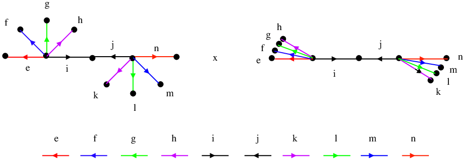
Recall that $g(e_{1}^{p})=e_{1}^{0}\overline{e_{2}^{q}}e_{2}^{0}$. We split the edge $e_{1}^{p}$ into $E$ and $E^{\prime}$ so that $g(E)=e_{1}^{0}\overline{e_{2}^{q}}$ and $g(E^{\prime})=e_{2}^{0}$. Split the edge $e_{2}^{q}$ into $F,F^{\prime}$ and $F^{\prime\prime}$ so that $g(F)=e_{2}^{0}$, $g(F^{\prime})=\overline{e_{2}^{0}}$ and $g(F^{\prime\prime})=e_{2}^{q}\overline{e_{1}^{0}}e_{1}^{1}$. For the template ${\mathcal{T}}_{(p,q)}$, we can use the symbols $\sf x_{i=0..p+1}$, and $\sf y$,$\sf z_{j=0...q+1}$ for the first star, and second star respectively. The edge $e_{1}^{0}$ goes to $\sf x_{0}$, and the edge $e_{2}^{0}$ goes to $\sf z_{0}$, etc., and $e_{1}^{p}$ is split into $\sf x_{p}$ and $\sf x_{p+1}$ corresponding to $E$ and $E^{\prime}$, and $e_{2}^{q}$ split into $\sf z_{q},\sf z_{q+1},\sf y$ corresponding to $F,F^{\prime}$ and $F^{\prime\prime}$. We denote the left end point and right end point of the branch segment of the strip $\sf x$ by $p_{\ell}(\sf x)$ and $p_{r}(\sf x)$ respectively. Since the initial vertex of $e_{1}^{0},e_{1}^{1},\cdots,e_{1}^{p}$ is the same vertex $q_{\ell}$, we must abstractly identify (1) $p_{r}(\sf x_{1})$, $p_{r}(\sf x_{2})$ ,$\cdots$, $p_{r}(\sf x_{p})$ and $p_{\ell}(\sf x_{0})$. In the same manner, we need to identify (2) $p_{r}(\sf x_{0})$ and $p_{\ell}(\sf y)$, (3) $p_{r}(\sf y)$ and $p_{\ell}(\sf z_{q+1})$, (4) $p_{r}(\sf z_{q+1})$ and $p_{\ell}(\sf z_{q})$, (5) $p_{\ell}(\sf z_{0})$, $p_{\ell}(\sf z_{1})$, $\cdots$, $p_{\ell}(\sf z_{q-1})$ and $p_{r}(\sf z_{q})$, and (6) $p_{\ell}(\sf x_{p})$ and $p_{r}(\sf x_{p+1})$.

For the remainder of the paper, we conveniently leave these boundary curves as distinct. When constructing subtemplates of this branched surface, we are careful never to use these edges within the subtemplates. In this way, we do not need to worry about the changes to the periodic orbits set we have made.

The normal form of ${\mathcal{T}}_{(p,q)}$ appears in cartoon form as in Fig. 12.

In order to construct ${\mathcal{U}}^{m}_{(p,q)}$, the template for the $m$-fold branched cover of ${\mathcal{T}}_{(p,q)}$, we must “peel off” a parallel copy of $\beta$ and cut ${\mathcal{T}}_{(p,q)}$ by a spanning disc for this unknot: cf. the figure-eight knot case in Fig. 4. Thus, the fundamental domain of ${\mathcal{U}}^{m}_{(p,q)}$ depends on the linking properties of $\beta$ with ${\mathcal{T}}_{(p,q)}$.

Proof: Note that $g_{(n_{1},n_{2})}$ has three fixed points $q_{\ell}$, $q_{c}$, $q_{r}$, where $q_{\ell}$ and $q_{r}$ are as above and $q_{c}\in e_{2}^{q}$ (see Lemma 3.6). These suspend to give the three unknots $k_{\ell}$, $k_{c}$, and $k_{r}$. It is clear from the image of the train track (see Figs. 10 and 14) that the fixed point $q_{c}$ is “in back” of the image of all the other edges, and that consequently the suspension of this fixed point, $k_{c}$, is an unknot which is of twist zero and separable from all other orbits on the template. Hence, $\ell k(k_{c},\beta)=0$. Since the train track map rotates each star about its central vertex with opposite orientations, it is easy to see that $\ell k(k_{\ell},\beta)=+1$ and $\ell k(k_{r},\beta)=-1$ (see Fig. 14[left]).

Since the strip $\sf y$ contains $k_{c}$ and $\ell k(k_{c},\beta)=0$, $\sf y$ and $\beta$ are linked as in Fig. 14. Because of the way we unfolded the star in Fig. 11, the way that $\sf z_{q+1}$ and $\beta$ are linked is same as that of $\sf y$ and $\beta$.

Notice that the edges $e_{1}^{0},\cdots,e_{1}^{p}$ were all “split off” of $q_{\ell}$, and $\ell k(k_{\ell},\beta)=+1$. Hence $\sf x_{0},\cdots,\sf x_{p},\sf x_{p+1}$ and $\beta$ are linked as in Fig. 14. Since the edges $e_{2}^{0},\cdots,e_{2}^{q-1},F(\subset e_{2}^{q})$ were also “split off” of $q_{r}$ and $\ell k(k_{r},\beta)=-1$, the strips $\sf z_{0},\cdots,\sf z_{q-1},\sf z_{q}$ and $\beta$ are linked as in Fig. 14. This completes the proof. ∎

By Lemma 4.1, the fundamental domain of ${\mathcal{U}}_{(p,q)}^{m}$ is as in Fig. 15, where we have cut along a spanning disc of $\beta$. To form ${\mathcal{U}}_{(p,q)}^{m}$, take $m$ copies of this fundamental domain joined cyclically end-to-end: see, e.g., Fig. 17.

The (very complicated) normal form ${\mathcal{U}}^{m}_{(n_{i},n_{i+1})}$ is tame compared to the full template ${\mathcal{U}}^{m}_{(n_{1},\ldots,n_{k})}$. Fortunately, we do not need to consider the most general case.

Proof: We prove this result on the level of the train track (by subdividing and removing extraneous portions), and then suspend this to obtain the result for subtemplates. We only prove the case $n_{i},n_{i+1}>1$, for other cases are similar. Let $G=G_{(n_{1},\cdots,n_{k})}$ and $g=g_{(n_{1},\cdots,n_{k})}$. For the proof of the lemma, it is enough to show that there exist subdivisions $I_{2}I_{1}=e_{i}^{n_{i}}$, $J_{3}J_{2}J_{1}=e_{i+1}^{n_{i+1}}$ of $G$ that satisfy the following:

Remove $I_{2}$ and $J_{2}$ from $S_{i}$ and $S_{i+1}$ respectively. Then $(S_{i}\cup S_{i+1})^{\prime}$ denotes the graph obtained from $(S_{i}\cup S_{i+1})$ by identifying the right end point of $J_{3}$ and the left end point of $J_{1}$. Then $g((S_{i}\cup S_{i+1})^{\prime})=g_{i+1}(g_{i}(S_{i}\cup S_{i+1}))$, see Fig. 16.

We demonstrate the case $i=1$, the proof for other cases being similar. Denote by $c_{i}$ the following edges of the train track: $c_{i}=e_{i}^{0}$ if $n_{i}=1$ and $c_{i}=\overline{e_{i}^{n_{i}}}e_{i}^{0}$ if $n_{i}>1$. By induction on $k$, one demonstrates that $g(e_{1}^{n_{1}})=e_{1}^{0}c_{2}\cdots c_{k}$, $g(e_{2}^{n_{2}})=e_{2}^{0}c_{3}\cdots c_{k-1}c_{k}\overline{c_{k}}~\overline{c_{k-1}}\cdots\overline{c_{2}}\overline{e_{1}^{0}}e_{1}^{1}$, and $g(e)=g_{2}(g_{1}(e))$ for $e\in S_{1}\cup S_{2}\setminus\{e_{1}^{n_{1}},e_{2}^{n_{2}}\}$. Take subdivisions $I_{2}I_{1}=e_{1}^{n_{1}}$ and $J_{3}J_{2}J_{1}=e_{2}^{n_{2}}$ such that $g(I_{1})=e_{1}^{0}c_{2}$, $g(J_{3})=e_{2}^{0}$, and $g(J_{1})=\overline{c_{2}}\overline{e_{1}^{0}}e_{1}^{1}$. Since $g(I_{1})=g_{2}(g_{1}(e_{1}^{n_{1}}))$, $g(J_{3})g(J_{1})=g_{2}(g_{1}(e_{2}^{n_{2}}))$ and $g(e)=g_{2}(g_{1}(e))$ for $e\in S_{1}\cup S_{2}\setminus\{e_{1}^{n_{1}},e_{2}^{n_{2}}\}$, we have $g((S_{1}\cup S_{2})^{\prime})=g_{2}(g_{1}(S_{1}\cup S_{2}))$. ∎

Proof: We consider the case of $i$ odd and $n_{i},n_{i+1}>1$; the other cases share identical proofs. The key step in this lemma is to determine the linking properties of $\beta$ with the subtemplate obtained from Lemma 4.2.

Note that $g_{(n_{1},\cdots,n_{k})}$ has three corresponding fixed points $q_{\ell}^{\prime},q_{c}^{\prime},q_{r}^{\prime}$, where $q_{\ell}^{\prime}$ and $q_{r}^{\prime}$ are $(n_{i}+1)$ vertex and $(n_{i+1}+1)$ vertex of $S_{i}$ and $S_{i+1}$ respectively, and $q_{c}^{\prime}\in e_{i+1}^{n_{i+1}}$. Denote by $k_{\ell}^{\prime}$, $k_{c}^{\prime}$, $k_{r}^{\prime}$ the three unknots given by suspending these points. Let $\beta$ and $\beta^{\prime}$ be the closures of $b_{(n_{1},n_{2})}$ and $b_{(n_{1},\cdots,n_{k})}$ respectively. As in the proof of Lemma 4.1, one shows that $\ell k(k_{\ell}^{\prime},\beta^{\prime})=\ell k(k_{\ell},\beta)=+1$, $\ell k(k_{c}^{\prime},\beta^{\prime})=\ell k(k_{c},\beta)=0$, and $\ell k(k_{r}^{\prime},\beta^{\prime})=\ell k(k_{r},\beta)=-1$, see Fig. 14(b). This together with Lemma 4.2 implies Lemma 4.3. ∎

We begin with the easiest and least general of the three Main Theorems. A proof can be obtained implicitly by a combination of Lemma 4.3 with a geometric argument from [14, pp. 444-5]. However, to set a pattern for the proofs of Main Theorems (a) and (b), we give a different proof of (c).

Proof: From Lemma 4.3, we may restrict attention to the subtemplate ${\mathcal{U}}^{m}_{(1,1)}$ within ${\mathcal{U}}^{m}_{(n_{1},\cdots,n_{k})}$. The template ${\mathcal{T}}_{(1,1)}$ is given in cartoon form in Fig. 4, along with a representation of the fundamental domain of ${\mathcal{U}}^{m}_{(1,1)}$. Our strategy is to identify three unknots on ${\mathcal{U}}^{m}_{(1,1)}$ — $\kappa$, $\kappa^{\prime}$, and $\kappa^{\prime\prime}$ — to which we can apply Theorem 2.4.

Specifically, using the symbolic representation of the orbits as periodic words, let $\kappa=\left(\sf y\right)$, $\kappa^{\prime}=\left(\sf x^{m}\right)$, and $\kappa^{\prime\prime}=\left(\sf z^{m}\right)$. Recall that $\left(\sf x^{m}\right)$ means to follow the periodic orbit which traverses the $\sf x$-strip $m$ times. While there is an ambiguity in the symbolic representation (in terms of which fundamental domain the symbol is on), the only choice is for $\left(\sf y\right)$, and by cyclic symmetry, the result is independent of the choice.

It is trivial to see from Fig. 17[left] that (1) these three curves are separable unknots; and (2) $\kappa$ has zero twist, $\kappa^{\prime}$ has positive twist, and $\kappa^{\prime\prime}$ has negative twist. The only other ingredient needed to invoke Theorem 2.4 is that the three orbits meet at a branchline as in Fig. 3. This is not the case, since the strip $\sf z$ does not fully cover the branchline. To remedy this, we replace $\left(\sf x^{m}\right)$ with $\left(\sf y\sf x^{m}\right)$. This orbit is still a separable unknot (using [13, Prop. 3.1.19]) whose (already positive) twist has increased by two and which now passes through the triple branchline in precisely the manner of Fig. 3. Hence, by Theorem 2.4, ${\mathcal{U}}^{m}_{(1,1)}$ is universal. ∎

The following theorem will allow us to completely classify the fibrations of 2-bridge knot complements in the next section.

Proof: To prove Theorem 5.2, it suffices to show that ${\mathcal{U}}^{2}_{(p,q)}$ is universal for all $p$ and $q$. We assume $p,q>1$, the other cases being both simpler and similar to Main Theorem (c). The strategy, as in the previous theorem, is to find three well-chosen unknots $\kappa,\kappa^{\prime},\kappa^{\prime\prime}$ on ${\mathcal{U}}^{2}_{(p,q)}$.

As before, choose $\kappa:=(\sf y)^{\infty}$ the untwisted unknot separable from all other orbits on the template. For $p$ odd (resp. even), define

see Fig. 18. For $q$ odd (resp. even), define

see Fig. 19. Note that there is an ambiguity as to which fundamental domain the orbit segment $y$ of $\kappa^{\prime}$ and $\kappa^{\prime\prime}$ passes through. We specify as follows: take $\kappa^{\prime}$ and $\kappa^{\prime\prime}$ such that the orbit segment $y$ passes through the fundamental domain where $\kappa$ lies. The figures imply that these are separable unlinked unknots with $\tau(\kappa)=0$, $\tau(\kappa^{\prime})>0$, and $\tau(\kappa^{\prime\prime})<0$. These unknots $\kappa,\kappa^{\prime}$ and $\kappa^{\prime\prime}$ pass through the triple branchline as in Fig. 20. Hence, by Theorem 2.4, ${\mathcal{U}}^{2}_{(p,q)}$ is universal. ∎

For part (a) of the Main Theorem — that the universal fibration property holds for $m$ sufficiently large — we give a more precise formulation.

Proof: By Lemma 4.3, it is enough to show that ${\mathcal{U}}_{(p,q)}^{m}$ is universal for each $m\geq N(N-1)$, where $N=\max\{p,q\}$. As before, we assume $p$ and $q$ greater than $1$.

Let $m=pt^{\prime}+s^{\prime}=qt^{\prime\prime}+s^{\prime\prime}$ be Euclidean integer factorizations of $m$; hence $0\leq s^{\prime}<p$ and $0\leq s^{\prime\prime}<q$. As $m\geq N(N-1)$, it follows that $t^{\prime}\geq s^{\prime}$ and $t^{\prime\prime}\geq s^{\prime\prime}$. Consider the following three periodic orbits on ${\mathcal{U}}_{(p,q)}^{m}$:

The orbit $\kappa$ is, as before, an untwisted unknot which lies within one fundamental domain of ${\mathcal{U}}_{(p,q)}^{m}$. The orbit $\kappa^{\prime}$ passes through $p(t^{\prime}-s^{\prime})+(p+1)s^{\prime}=pt^{\prime}+s^{\prime}=m$ fundamental domains of ${\mathcal{U}}_{(p,q)}^{m}$. Except for the occasional excursions about the $\sf y$ orbit (which do not change the knot type), the orbit $\kappa^{\prime}$ can be thought of as a 1-strand braid about the braid axis of ${\mathcal{U}}_{(p,q)}^{m}$: it is therefore an unknot. All twisting in the $\sf x$-strips is of a positive nature, so that $\kappa^{\prime}$ is an unknot with positive twist. A similar argument shows that $\kappa^{\prime\prime}$ passes through $q(t^{\prime\prime}-s^{\prime\prime})+(q+1)s^{\prime\prime}=m$ fundamental domains and is an unknot with negative twist separable from $\kappa^{\prime}$.

These orbits are a triple of separable unknots which satisfy the conditions of Theorem 2.4, as illustrated in Fig. 21. Hence ${\mathcal{U}}_{(p,q)}^{m}$ is universal. ∎

Recall that a 2-bridge knot is one which can be isotoped so as to have precisely four critical points (two minima and two maxima) with respect to the standard height function in $\mathbb{R}^{3}$. We can affirmatively answer Question 6.1 in this category.

Proof: The work of Gabai and Kazez [12] explicitly shows that the class of fibred 2-bridge knots is precisely that class of knots whose fibres are a chain of plumbed Hopf bands, and that the monodromy is of pseudo-Anosov type if and only if the Hopf bands are not all of the same sign, which is to say, if and only if it is not a torus knot. We claim that such a chain of plumbed Hopf bands has a closed braid form of $({b_{(n_{1},\cdots,n_{k})}})^{2}$. The proof is inductive on the number of Hopf bands and illustrated in Fig. 22. The key step is noting that the fibre for the closure of $({b_{(n_{1},\cdots,n_{k})}})^{2}$ is a stack of discs attached by a pairs of half-twisted bands: this is precisely a chain of plumbed Hopf bands. From Theorem 5.2, we have that this knot must be universally fibred. ∎

We can enlarge the class of universally fibred knots considerably by taking connected sums.

Proof: In [11, Corollary 1.4.], it is shown that the Murasugi sum of fibre surfaces is “natural”. Specifically, if $K_{i}$ is a fibred knot/link ($i=1,2$) with fibre surface $\Sigma_{i}$ and monodromy $\Phi_{i}$ satisfying $\Phi_{i}|_{\partial{\Sigma_{i}}}=id$, then the Murasugi sum of $\Sigma_{1}$ and $\Sigma_{2}$ along a $2k$-gon $D$ common to $\Sigma_{1}$ and $\Sigma_{2}$ is fibre surface and has monodromy $\tilde{\Phi}_{1}\circ\tilde{\Phi}_{2}$, where $\tilde{\Phi}_{i}$ is equal to $\Phi_{i}$ on $\Sigma_{i}$ and the identity map elsewhere.

Even more importantly, the proof of this result uses vector fields transverse to the fibration to achieve the result. Thus, we actually have that a transverse vector field of the Murasugi sum decomposes naturally.

The simplest kind of Murasugi sum (where the attachment is along a 2-gon in the spanning surfaces) is precisely the connected sum. Choose the monodromy $\Phi_{1}$ of the universally fibred knot to be the pseudo-Anosov representative, isotoped so as to be the identity map on the the boundary. Likewise, choose the monodromy $\Phi_{2}$ to be the Thurston canonical form isotoped to be the identity on the boundary. The composition monodromy on the connected (in this case, Murasugi) sum is easily isotoped to have an invariant curve separating the universal pseudo-Anosov component from the Thurston form of $\Phi_{2}$. Thus, the theorem of Asimov and Franks implies that any transverse vector field must have at least this set of periodic orbits — all knots and links. ∎

As a corollary of the proof, we see that in certain instances, more general Murasugi sums (e.g., plumbing) can preserve the universal fibration property as well. One would need to control (1) the dynamics on the attaching region, to preserve the pseudo-Anosov property of the monodromy, and (2) the location of the attaching region, so that it does not interfere with the universal subtemplate.

We believe that there are pseudo-Anosov fibred knots or links whose monodromies are too “twisted” to admit a universal template in the suspension. Our proposed example stems from the fact that the proof of Main Theorem (c) requires a sufficiently high order branched cover.

Our reason for conjecturing the non-universality stems from the difficulty in finding enough unknotted orbits on which to build a universal subtemplate.

References

- [1] D. Asimov and J. Franks, Unremovable closed orbits, in Geometric Dynamics, Ed. J. Palis, Lect. Notes in Math. 1007, Springer-Verlag, (1983) 22-29.
- [2] M. Bestivina and M.Handel, Train-Tracks for surface homeomorphisms, Topology 34 (1) (1994) 109-140.
- [3] J. Birman, A representation theorem for fibered knots and their monodromy maps, in Topology of Low-dimensional Manifolds, Lecture Notes in Math. 722, Springer-Verlag (1977) 1-8.
- [4] J. Birman and R. Williams Knotted periodic orbits in dynamical systems – I: Lorenz’s equations, Topology 22(1), (1983) 47-82.
- [5] J. Birman and R. Williams, Knotted periodic orbits in dynamical systems – II: Knot holders for fibered knots, Contemp. Math. 20, (1983) 1-60.
- [6] A. de Carvalho and T. Hall, Braid forcing and star-shaped train tracks, preprint ArXiv math.DS/0204115, 2002.
- [7] J. Casasayas, J. Martinez Alfaro, and A. Nunes, Knots and links in integrable Hamiltonian systems, J. Knot Theory & Ramifications 7(2) (1998) 123-153.
- [8] J. Etnyre and R. Ghrist, Gradient flows within plane fields, Commun. Math. Helv. 74 (1999) 507-529.
- [9] A. Fomenko and T. Z. Nguyen, Topological classification of integrable nondegenerate Hamiltonians on isoenergy three-dimensional spheres, in Adv. Soviet Mathematics Vol. 6, A. Fomenko ed., pp. 267-296, AMS, 1991.
- [10] J. Franks, Knots, links, and symbolic dynamics, Ann. Math. 113 (1981) 529-552.
- [11] D. Gabai, The Murasugi sum is a natural geometric operation. II, Contemp. Math. 44, (1985) 93-100.
- [12] D. Gabai and W. Kazez Pseudo-Anosov maps and surgery on fibred -braidge knots, Top. & Its Applications 37 (1990) 93-100.
- [13] R. Ghrist, P. Holmes and M. Sullivan, Knots and Links in Three-Dimensional Flows, Lect. Notes in Math. 1654, Springer-Verlag (1997).
- [14] R. Ghrist, Branched two-manifolds supporting all links, Topology 36 (2) (1997) 423-448.
- [15] D. Goldsmith, Symmetric fibered links, in Knots, Groups, and -Manifolds, Ann. of Math. Studies 84, Princeton Univ. Press, Princeton, (1975) 3-23.
- [16] P. Melvin and N. Tufillaro, Templates and framed braids Phys. Rev. A, 44(6) (1991) 3419-3422.
- [17] H. Morton and M. Rampichini, Mutual braiding and the band presentation of braid groups, in Knots in Hellas ’98 Delphi, 335-346.
- [18] R. Penner and J. Harer, Combinatorics of Train Tracks, Ann. of Math. Studies 125, Princeton Univ. Press, Princeton (1992)
- [19] D. Rolfsen, Knots and Links, Publish or Perish Press, 1976.
- [20] W. Thurston, On the geometry and dynamics of diffeomorphims of surfaces, Bull. Am. Math. Soc. 19 (2) (1988) 417-431.
- [21] M. Wada, Closed orbits of nonsingular Morse-Smale flows on , J. Math. Soc. Japan 41(3) (1989), 405-413.
- [22] R. Williams, One dimensional nonwandering sets, Topology, 6 (1967), 473-487.