Zigzag Structures of Simple Two-faced PolyhedraResearch financed by EC’s IHRP Programme, within the Research Training Network “Algebraic Combinatorics in Europe,” grant HPRN-CT-2001-00272.
Abstract
A zigzag in a plane graph is a circuit of edges, such that any two, but no three, consecutive edges belong to the same face. A railroad in a plane graph is a circuit of hexagonal faces, such that any hexagon is adjacent to its neighbors on opposite edges. A graph without a railroad is called tight. We consider the zigzag and railroad structures of general -valent plane graph and, especially, of simple two-faced polyhedra, i.e., -valent -polytopes with only -gonal and -gonal faces, where ; the main cases are , and (the fullerenes).
We completely describe the zigzag structure for the case =. For the case = we describe symmetry groups, classify all tight graphs with simple zigzags and give the upper bound for the number of zigzags in general tight graphs. For the remaining case = we give a construction realizing a prescribed zigzag structure.
Mathematics Subject Classification. Primary 52B05, 52B10;
Secondary 05C30,
05C10.
Key words. Two-faced polyhedra, plane graphs, zigzags, point groups.
1 Introduction: main notions
A graph consists of a vertex-set and an edge-set , such that either one or two vertices are assigned to each edge as its ends. A graph is said to be simple if no edge has only one end-vertex and no two edges have identical end-vertices. A plane graph is a particular drawing of a graph in the Euclidean plane using smooth curves that cross each other only at the vertices of the graph. A graph, which has at least one such drawing, is called planar. We only deal with simple connected plane graphs, whose vertex-sets and edge-sets are finite.
By a polyhedron we mean a convex -dimensional polytope. The vertices and the edges of a polyhedron form a simple planar -connected graph called skeleton. Such a graph has a unique drawing (up to diffeomorphisms of the Euclidean plane), but there exist many distinct polyhedra having this graph as their skeleton; all such polyhedra are of the same combinatorial type. The group of isometries of a polyhedron (so-called point group) is a subgroup of the algebraic symmetry group of the graph. By a theorem of Mani ([Ma71]), there is, for each combinatorial type, at least one polyhedron, for which this inclusion becomes equality. So, we can identify the polyhedron and its graph, as well as the algebraic symmetry group and the point group.
The -vector of a polyhedron enumerates the numbers of vertices of degree . A polyhedron is simple if for . The -vector of a polyhedron counts the numbers of faces having sides. For a connected plane graph , we denote its plane dual graph by and define it on the set of faces of with two faces being adjacent if they share an edge. Clearly, and .
Let be a plane graph, such that every of its vertices has at least degree . Then all edges, incident to a vertex , can be labeled in counter-clockwise order as , where is the degree of in . For any edge , , the edges , and (with and being addition modulo ) are called, respectively, the left and the right. A circuit of edges of is called a zigzag (or a Petrie path [Cox73], geodesic [GrünMo63], left-right path [Sh75]), if, in tracing the circuit, we alternately select, as the next edge, the left neighbor and the right neighbor (see Figure 1). In a -valent plane graph, any pair of edges sharing a vertex define a zigzag.
Given an edge, there are two possible directions for extending it to a zigzag. Hence, each edge is covered exactly twice by zigzags. A zigzag is called simple if it has no self-intersection. Otherwise, it has at least one edge, say, , in which it self-intersects. Let us choose an orientation on ; call the edge of type I or type II [GrünMo63] if traverses it twice in the opposite or in the same direction, respectively (see Figure 1). Clearly, the type of edge does not depend on the choice of orientation. Edges of type I and type II correspond to edges of cocycle and cycle character in [Sh75]. The signature of a zigzag is the pair , where and are the numbers of its edges of type I and type II, respectively.
The -vector of a graph is the vector enumerating the lengths of all its zigzags with their signature as subscript. The simple zigzags are put in the beginning, in increasing order of length, without their signature , and separated by a semicolon from others. Self-intersecting zigzags are also ordered by increasing lengths. If there are zigzags of the same length and the same signature , then we write . For a zigzag , its intersection vector is such that is an increasing sequence of sizes of its intersection with all others zigzags, and denote respective multiplicities.
The length of each zigzag is even, because we consecutively take left and right turns. But the length of intersection of two simple zigzags can be odd (see Klein and Dyck maps on the Table 1; they both have oreinted genus and come as quotients of regular triangulations of the hyperbolic plane having valency and , respectively). Returning to our plane case, the number of intersection can be even only.
A graph is called -uniform if all zigzags have the same length and signature, -transitive if its group acts transitively on zigzags. Clearly, -transitivity implies -uniformity. A graph is called -knotted if it has only one zigzag, -balanced if all its zigzags of the same length and same signature, have identical intersection vectors. Clearly, -transitivity implies -balancedness.
Let , …, be all zigzags of . On every zigzag choose an orientation; there are possibilities. Every edge, being covered twice by zigzags (one or two), can be, with respect to the choosen orientation of all zigzags, oriented in the opposite or same direction. We call such an edge of type I or type II with respect to the fixed orientation. If an edge is a self-intersection edge of some zigzag, then the notion of type is independent of the fixed orientation and coincides with the notion of type I and II, which was introduced above.
While for dual graphs - and -vectors are interchanged, the -vector remains the same, except that type I and type II in the signature are interchanged. Other kinds of dualities (for example, interchanging - and -vector, but preserving -vector) are considered in [Li82].
The medial graph of is defined on the set of edges of with two edges being adjacent if they share a common vertex and if they belong to a common face. The medial graph is -valent and . Zigzags of and correspond to central circuits (see below) of . Any -valent plane graph is the medial graph for a pair of mutually dual plane graphs: one can assign two colors to the faces of in the “chess way”, such that no two adjacent faces of have the same color. Two faces of the same color are said to be adjacent if they share a vertex.
In general, a central circuit of an Eulerian (i.e., having only vertices of even degree) plane graph is a circuit, which is obtained by starting with an edge and continuing at each vertex by the edge opposite to the entering one. A link is one or more circles (components of a link) embedded into the space ; a link with one component is called knot. A projection of a link is a drawing of it on the plane with gaps representing underpass and solid line representing overpass. If a drawing of a link has alternating underpasses and overpasses, then it is called alternating; so, we can see it just as a -valent plane graph. We will consider only minimal projections, i.e., those without -gons (loops). Clearly, each edge belongs to exactly one central circuit and any -valent graph without -gons can be seen as a minimal projection of an alternating link with components corresponding to its central circuits. Since zigzags in correspond to central circuits in , each zigzag corresponds to a component of the corresponding alternating link. The bipartition of edges of a -knotted graph into type I and type II corresponds to a bipartition of the vertices of its medial graph (which is a projection of an alternating knot).
Call a polyhedron two-faced if it has only - and -gonal faces with . In particular, denote -valent two-faced -vertex polyhedron by , , if =, , , respectively. Given two circuits and , an -sided prism is formed when every is joined to by an edge. Now, an -sided antiprism is formed by adding the cycle ,,,, …, ,,,.
A point group is a finite subgroup of the group of isometries of the space , fixing the origin. The connection with plane graphs come from representing them on the sphere centered at the origin. The list of point groups is splitted into two classes: the infinite families and the sporadic cases. Every point group contains a normal subgroup formed by the rotations of . The group, denoted , is the cyclic group of rotations by angle with around a fixed axis . Both groups and contains as normal subgroups of rotations. The group (respectively, ) is the group, generated by and a symmetry of plane , with being orthogonal to (respectively, containing ). The group is the group, generated by and a rotation by angle , whose axis is orthogonal to . The point group (respectively, ) is generated by and a rotation by angle , whose axis is orthogonal to and contained in a plane of symmetry (respectively, going between two planes of symmetry). Both, and , contain as a normal subgroup. If is even, one defines the point group to be the cyclic group generated by the composition of a rotation by angle with axis and a symmetry of plane with being orthogonal to . The particular cases , and correspond to the trivial group, the plane symmetry group and the central symmetry inversion group. The point groups , and are the symmetry group of the Tetrahedron, Cube and Icosahedron; the point groups , and are their normal subgroup of rotations. The point group is formed by all and with . More detailed description of point groups are available, for example, from [FoMa95] and [D1].
| # edges | Polyhedron | -vector | Int. vector |
|---|---|---|---|
| 6 | Tetrahedron | ||
| 12 | Cube | ||
| 12 | Octahedron | ||
| 30 | Dodecahedron | ||
| 30 | Icosahedron | ||
| 24 | Cuboctahedron | ||
| 60 | Icosidodecahedron | ||
| 48 | Rhombicuboctahedron | ||
| 120 | Rhombicosidodecahedron | ||
| 72 | Truncated Cuboctahedron | ||
| 180 | Truncated Icosidodecahedron | ||
| 18 | Truncated Tetrahedron | ||
| 36 | Truncated Octahedron | ||
| 36 | Truncated Cube | ||
| 90 | Truncated Icosahedron | ||
| 90 | Truncated Dodecahedron | ||
| 60 | Snub Cube | ||
| 150 | Snub Dodecahedron | ||
| 3m | , | ||
| 3m | , | ||
| 3m | , | ||
| 4m | |||
| 4m | |||
| 84 | Klein map | ||
| 48 | Dyck map |
In Table 1, zigzag notions are illustrated by the regular and semiregular polyhedra (i.e., such that their symmetry group is transitive on vertices). This table is a slightly more precise version (indicating types of self-intersection of zigzags) of Table 1 of [DHL02]. It is easy to see that for self-intersecting zigzags of prisms and antiprisms, the self-intersections of type I, if any, occur on the edges of the two -gons, while those of type II occur on other edges.
The notion of a zigzag was generalized to locally-finite infinite planar -connected graphs. All such edge-transitive graphs without self-intersecting zigzags (i.e., simple circuits and doubly infinite rays are the only zigzags) were classified in [GrSh87]: these are the three regular partitions , , of the Euclidean plane, the Archimedean partition , its dual and several infinities of partitions of the hyperbolic plane. Also the notion of zigzag (Petrie polygon) was extended in [Cox73] p. 223 for -dimensional polytopes and honeycombs.
This paper is based on extensive computation; in particular:
- (i)
- (ii)
- (iii)
2 General results for plane graphs
Theorem 2.1
For any planar bipartite graph there exist an orientation of zigzags, with respect to which each edge has type I.
Proof. We represent the graph on the sphere. The list of vertices, adjacent to a given vertex, can be organized in counter-clockwise order.
Let the vertex-set be partitioned into the two subsets and of the bipartition. Fix a zigzag ; it will turn left at vertices, say, and right at vertices . It is easy to see that the edges of self-intersection of can be only of type I.
Take another zigzag , having a common edge with . We choose an orientation on , such that is an edge of type I. Then will turn left at vertices and right at vertices . Iterating this construction, all zigzags will be oriented and all edges will have type I with respect to this orientation of zigzags.
In the case of one zigzag, this result was already known ([Sh75]). This theorem is also valid for any bipartite graph, which is embedded in an oriented surface, in view of the well-known topological fact that any two-dimensional orientable manifold admits coherent orientation of its faces.
Proposition 2.2
([DDF02]) Let be a plane graph; for any orientation of all zigzags of , we have:
(i) The number of edges of type II, which are incident to any fixed vertex, is even.
(ii) The number of edges of type I, which are incident to any fixed face, is even.
Proof. (i) For each vertex the number of times, that a zigzag enters it, should be equal to the number of times that a zigzag leaves it.
(ii) Passing to the dual graph, the type of edges are interchanged.
A consequence of the above proposition for any -valent plane graph (see [DDF02]) is that the set of vertices can be partitioned into two classes, say, class I and class II, where class I stands for vertices, which are incident to three edges of type I, and class II stands for vertices, which are incident to one edge of type I and two edges of type II. If denotes the number of vertices of and denotes the number of its vertices of class I, then the number of edges of type I is . Clearly, the number of edges of type II is equal to the number of vertices of class II, i.e., to .
It was conjectured in ([DDF02]) that any -valent plane graph, which is -knotted, has an odd number of edges of type I. The condition of -valency is necessary: for example, the -bipyramid (i.e., ) has -vector .
Clearly, any graph with , or zigzags is -balanced. See smallest -unbalanced -valent graph and graphs of type , on Figure 2. We did computations trying to find an example of a -unbalanced and -uniform -valent polyhedron (for ), graph of type (for ) and (for ); surprisingly, we did not find any such example.

-vertices graph ,

Graph (),

Graph (),
In the rest of this section, we give a local Euler formula for zigzags. Let be a plane -valent graph. Consider a patch in , which is bounded by arcs (i.e., paths of edges) belonging to zigzags (different or coinciding).
We admit also -gonal patch , i.e., just the interior of a simple zigzag. Suppose that the patch is regular, i.e., the continuation of any of its bounding arcs (on the zigzag, to which it belongs) lies outside of the patch (see Figure 3). Let be the -vector enumerating the faces of , which are contained in the patch .
There are two types of intersections of arcs on the boundary of a regular patch: either intersection in an edge of the boundary, or intersection in a vertex of the boundary. Let us call these types of intersections obtuse and acute, respectively (see Figure 3); denote by and the respective number of obtuse and acute intersections. Clearly, , where is the number of arcs forming the patch.
Theorem 2.3
Let be a -valent plane graph (-gonal and -gonal faces are permitted). If is a regular patch, then the following equality holds
Proof. Let be the induced plane subgraph of formed by the patch . The vertices of have degree or ; we denote their respective number by and . The exterior face is -gonal, where is the length of the boundary of the patch. Direct enumeration gives the following expressions for the number of edges of
Euler’s formula, applied to the plane graph , yields
The above two expressions of give
Eliminating yields
For example, if the patch is a -gon (i.e., if it is bounded by a simple zigzag), then and we get
Denote by and the numbers of vertices on the boundary of , having degree and , respectively. Clearly, and .
Now we use that is a regular patch. Specifying acute and obtuse types of arc intersections on the boundary of , we get , which gives
Corollary 2.4
Let be a -valent plane graph. Let be a -gonal regular patch with -vector in . Then we have:
(i) If has no -gonal faces with , then .
(ii) If is a two-faced graph , , then
Proof. (i) By the above theorem
which gives the result. (ii) also follows by direct application of Theorem 2.3.
3 Railroads and pseudo-roads
Let be a plane graph. Call a railroad of a circuit of hexagonal faces in , such that each hexagon is adjacent to its neighbors on opposite edges (in [GrünMo63], a simple, i.e., without self-intersections, railroad is called a belt). Clearly, a railroad is bounded by two “parallel” (concentric if the railroad is simple) zigzags. The graph is called tight if it has no railroads. A railroad in corresponds to a central circuit in , which goes only through -valent vertices.
We associate to each railroad a representing plane curve in the following way: in each of its hexagons one connects, by an arc, the midpoints of opposite edges, on which it is adjacent to its two neighbors. The sequence of those arcs can be seen as a Jordan curve in the plane and self-intersections of railroad correspond to self-intersections of the curve.
Those self-intersections can be only double or triple, because a railroad consists of hexagons. If the railroad has no triple self-intersection points, then this curve can be seen as a projection (not minimal, if there are -gons) of an alternating knot (see, for example, [Kaw96] and [Rol76]) with crossings, where is the number of self-intersection points. If there are several railroads without triple intersections and triple self-intersections, then the set of plane curves, representing them, can be seen as a projection of an alternating link.
A set of railroads can be seen as a plane graph with valency or of its vertices, accordingly to double or triple points of intersection or self-intersection of the curves. Every -gonal face of can be viewed as a regular patch with intersections of arcs. In the case, when has no -gonal faces with , Corollary 2.4.(i) implies that .
A railroad is bounded by two zigzags and , which have the same length and signature. Each edge of self-intersection of , corresponds to a self-intersection of and so, to an hexagon of self-intersection of . Since can self-intersect in an edge of type I or type II, there are two types of double self-intersections of railroad. Simple analysis yields two types for triple self-intersections of railroad: either self-intersects in three edges of type I or it self-intersects in one edge of type I and two edges of type II. See Figure 4 for all possibilities.
Graph

Graph

Graph
In order to illustrate the notion of railroads, we give in the remainder of this section two lists: those having, or, respectively, not having, triple self-intersections of the curves representing railroads in two-faced -vertex polyhedra of type for small . In Tables 2 and 3, we present the first cases of such curves; the first column being the name of the curve. The smallest graph of type , which is denoted by , being the number of the graph in CPF output (see [Ha]), is listed in the column “First appearance”. In some cases the curve appears twice in this graph; we mark this situation by putting “twice” in parenthesis. The third and fourth column give the number of intersection points and the number of -gons, . Columns “Group” and “-vector” give the point group and the -vector of the corresponding graph of type .
The computation of all railroads in the class of polyhedra , , with at least two self-intersections, all being double self-intersections, produced a list of projections of alternating knots presented in Table 2. We use Rolfsen’s notation, see [Rol76], for knots with at most crossings and those of Thistlethwaite ([Thi]), for other knots. We denote by and the - and -crossing alternating knots, appearing in a graph of type , which are and , respectively. (The knot comes from or from knot by inscribing consecutively or triangles, respectively.) All curves, representing railroads with triple self-intersections in the graphs , with are given in Table 3. The notation , given in first column, means that is the number of triple points of the curve and is order of appearance (amongst curves with triple points) in this table.
![[Uncaptioned image]](0212352v2/ZZint111Railroad066_11.png)
Graph ,
![[Uncaptioned image]](0212352v2/ZZint111Railroad108_18.png)
Graph ,
![[Uncaptioned image]](0212352v2/ZZint111Railroad108_48.png)
Graph ,
Three graphs of type with triple self-intersecting railroads.
Remark 3.1
Let be a zigzag of signature bounding a railroad with double and triple self-intersections. Then one has .
Proposition 3.2
Let be a simple polyhedron with -vector and let be tight. Then the number of zigzags of is at most
Proof. In fact, each zigzag has a non -gonal face on each of its sides, since, otherwise, it would have a railroad on this side; so, the total number of incidences between zigzags and non -gons is at least twice the number of zigzags. On the other hand, the number of those incidences is exactly .
Proposition 3.3
Let be a graph of type , having railroads , …, ; let be a plane graph formed by the curves representing those railroads. Then:
(i) Every -gonal face of with contains exactly -t -gons of ; every -gonal face of contains one or two -gons of .
(ii) If is the number of -gonal faces of , then one has the inequality
Proof. Every -gonal face of can be viewed as a regular patch with (obtuse and acute) intersections of arcs. Let be the number of -gons inside . We will apply Theorem 2.3.
(i) If , then and we are done. If , then
Since is even, we get that , i.e., every -gon contains exactly two -gons. If , then
This yields or .
(ii) Any graph of type has six -gons; so, the result follows.
The Euler formula for the -vector of a -valent polyhedron, , is a discrete analog of the Gauss-Bonnet formula, , for the Gaussian curvature of a surface of genus . So, the -gons can be seen as positively curved, flat, or negatively curved, if , , or , respectively.
Consider a two-faced graph , which is a , or ; it has four -gons, six -gons, or twelve -gons, respectively. Let us call the graph of curvatures of the following graph (possibly, with loops and multiple edges) having as vertex-set all non -gonal faces of . Two vertices, say, non -gonal faces and of are called adjacent if there exist a pseudo-road connecting faces and . A pseudo-road is a sequence of hexagons, say, , …, , such that putting and , we have that any , , is adjacent to and on opposite edges. Clearly, the graph of curvatures of a graph , , is regular of degree .
Given an hexagon in a graph of type , , , any pair of opposite edges belongs to a railroad or a pseudo-road; so, we exactly have a triple covering of the set of all hexagons by the set of all railroads and pseudo-roads. Every non -gonal face, i.e., -gonal face with , has adjacencies with the system of pseudo-roads.
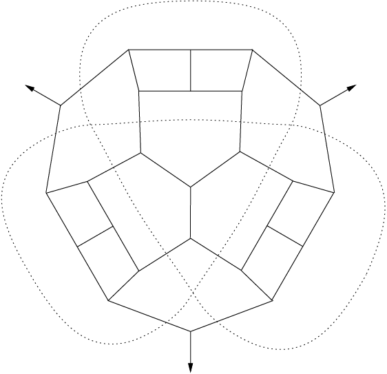
For the special case, when our graph is of type , any pseudo-road arriving on a -gonal face can be extended on the opposite edge. So, the set of such extended pseudo-roads, together with the set of railroads, can be identified with the set of central circuits of the dual of our graph. Hence, extended pseudo-roads can be seen (in the same way as it was done for railroads) as projections of a Jordan curve on the plane with double and, eventually, triple points of self-intersection. Those notions are illustrated in Figure 6. This graph has the following road decomposition: five concentric simple railroads (we indicate only the central, equatorial one), two self-intersecting railroads (they differ only by their opposite position on the sphere; we present only one of them) and all pseudo-roads.

One of two self-intersecting railroads and the equatorial simple railroad

All twelve pseudo-roads
4 Two-faced polyhedra
Remind that two-faced polyhedra have only - and -gonal faces with (see [DeGr99]). Denote by and the number of -gonal and -gonal faces.
Any -valent -vertex two-faced polyhedron has edges and satisfies the Euler relation , i.e., and . So, is possible only for simple polyhedra with (), (Dürer’s Octahedron), (four dual deltahedra). The other cases, namely, are denoted by , , , where is the number of vertices. The polyhedra are the well known fullerenes (of Organic Chemistry). See Table 4 for all the possibilities. The criterion for the existence of the polyhedra of type , and is due to [GrünMo63].
For the types , and in Table 4 the case yields the Tetrahedron, the Cube and the Dodecahedron. Those three polyhedra, together with dual deltahedra and , are the duals of the eight convex deltahedra. Dürer’s Octahedron is the Cube truncated at two opposite vertices. The four dual deltahedra from the fourth line of Table 4 are: (dual -bipyramid), dual bisdisphenoid, dual -augmented , dual -capped . Those four dual deltahedra, preceded by the Dürer’s Octahedron and , are given in Figure 7 with their -vectors and groups.
Lemma 4.1
Any connected -valent plane graph, having only -gonal faces with , is -connected.
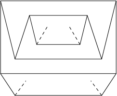
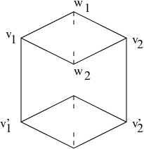
Proof. Let be one such graph and assume that there is one vertex , such that is disconnected. has two or three components; clearly, it cannot have three components, since . Denote by and the two components and by the edge linking to . Then two edges from will connect to another vertex and two edges from will connect to another vertex , since we assume that the faces are incident to at most edges. See below the corresponding drawing.
But the vertex will disconnect the graph and so, iterating the construction, we obtain an infinite sequence , …, of vertices that disconnect . This contradicts to initial assumption and proves that is -connected.
Denote by the -valent plane -vertex graph, whose faces are (organized in pairs of adjacent ones) triangles and hexagons. The graph is -connected but not -connected, its -vector is ; its symmetry group is or , if is even or odd, respectively. The first occurrences are depicted in Figure 8.
Proposition 4.2
Any -valent plane graph having only -gonal faces with , is -connected, except the graphs of the family .
Proof. Let be a -valent plane graph with -gonal faces, and assume that it is not -connected. Then there are two vertices, say, and , such that is disconnected. If has three components, then since , it is of the form depicted in Figure 9.a), which is impossible by the condition ; so, has two components, say, and .
There are two edges, say, and , that connect to . Since is disconnected, and are both incident to faces and . Then, by our assumption on size of faces, we get the following possibilities:
Only first two cases are possible, since, otherwise, we would have a non -connected plane graph. See in Figure 9.b),c) the possible continuation of those graphs.
In case b) one obtain an infinite structure; so, we get again a contradiction.

a)
b)
c)
Let us consider now the case c); the two points, and , can, either be connected by an edge and we are done, or be non-connected, in which case and disconnect the graph. In the latter case, one can iterate the construction. Since the graph is finite, the construction eventually finish and we get a graph , .
All graphs of type , , with maximal pair of symmetry ( or , or , or , respectively) are known; in fact, the Goldberg-Coxeter construction, denoted ([Cox71], [Gold37], [DD03]), implies that any graph of this type , , and those symmetry are of the form with and being Tetrahedron, Cube or Dodecahedron, respectively. Those graphs have vertices with , or , respectively. Those graphs are tight if and only if ; they are of symmetry , or if and only if or .
The polyhedra dual to the -valent polyhedra without -gonal faces, , are studied in [Thur98]; they are called there non-negatively curved triangulations (actually, the reference [Sah94] is an application of a preliminary version of [Thur98]). Theorem 3.4 in [Sah94] implies that , and , where denotes the number of polyhedra for , respectively.
5 Polyhedra
We present in Table 5 the numbers of and the numbers of tight for .
In [GrünMo63] it was shown that each zigzag in a graph of type is simple and a general construction of all was given; we sketch this construction with slightly different notation. If a zigzag contains two edges, say, and , of a triangle, then its third edge, say, defines a pseudo-road that finish on another triangle. Denote by one fourth of the length of the zigzag; then is the number of hexagons of . Consider the sequence of concentric simple railroads, which, possibly, goes around the patch depicted in Figure 10; let denote the number of zigzags and be the number of corresponding railroads. The same patch (with the same number of hexagons between the other two triangles and with the same number of concentric simple railroads, going around it) occurs on the other side of the sphere. As in [GrünMo63], we get, by direct computation, the equality and , where is the number of hexagons. See Figure 11.c),d) for two examples with and .
Take a triangle and an edge of this triangle; belongs to a sequence of adjacent -gons, which is concluded by another triangle . If one considers the three edges , , , then we obtain three triangles , , , respectively, that may be distinct or not.
Theorem 5.1
Any graph has exactly one of the following forms:
(i) The Tetrahedron or the Truncated Tetrahedron (the only case, when an hexagon is adjacent to more than two triangles).
(ii) There are two hexagons, every of which is adjacent to two triangles on opposite edges; there are one or two such graphs of type depending on or , respectively. Their symmetry groups are, respectively, if and , if .
(iii) There are four hexagons (in two adjacent pairs), every of which is adjacent to two triangles on non-opposite and non-adjacent edges; there is exactly one such graph for every , .11 1 In the exceptional case , there are only two polyhedra : the Cube truncated at four non-adjacent vertices and the Cube truncated at four vertices of two opposite edges. The second polyhedron is the unique and only example, which is of type (ii) and (iii). The symmetry group is or if is even or odd, respectively.
(iv) Each hexagon is adjacent to at most one triangle; there is an one-to-one correspondence between such graphs , having isolated triangles, and IPT fullerenes (i.e., those having their pentagons organized in triples of mutually adjacent ones).
Proof. For given graph of type , denote by the maximal number of triangles, which are adjacent to a hexagon. The only graph of type without hexagons is the Tetrahedron. The case corresponds to the -connected but not -connected -vertex plane graph (see Figure 8). The only graph of type with is the Truncated Tetrahedron. If , then two cases occur: either two triangles are adjacent to an hexagon on opposite edges or they are adjacent to an hexagon on non-opposite and non-adjacent edges.
The first case corresponds to the case of the Grünbaum-Motzkin construction. The divisibility of by follows from the formula . At the last step of the Grünbaum-Motzkin construction, namely, after adding railroads, we add a pair of triangles in one of two possible ways. If , then both ways give isomorphic graphs, both of symmetry , for (see Figure 11.b), for this possibility). If , then we get two non-isomorphic graphs, one of symmetry , the other of symmetry (see Figure 11.c),d) for those two possibilities).
Let our graph be of type (iii), i.e., two hexagons , are adjacent to two triangles , on non-opposite and non-adjacent edges, as in the picture below.
These two hexagons , are adjacent, respectively, to two hexagons , . By replacing the patch , , , by two triangles, one gets a graph , which is also of type (iii). By induction, one gets, for any with , an unique graph. A graph of type (iii) has two pairs of hexagons, each pair being adjacent to two triangles; if one does the operation, depicted above, to the two pairs, then the symmetry group remains the same. So, one has a periodicity of order for the symmetry groups and the result on groups follows.
If the graph has , then the operation, depicted in picture below, on all triangles realize a one-to-one correspondence.
See Figure 11.a),c),d) for all graphs having hexagons adjacent to two triangles.

a) vertices, case (iii),

b) vertices, case (ii),

c) vertices, case (ii),

d) vertices, case (ii),
Proposition 5.2
The graph of curvatures of a is one of the three following -vertex graphs:
Proof. Take a triangle, say, and an edge of . The pseudo-road, which is defined by and , establishes an edge between and, say, ; this pseudo-road is bounded by one zigzag . This zigzag belongs to a sequence of concentric zigzags . The zigzag defines a pseudo-road between the remaining triangles and , i.e., an edge connecting to in the graph of curvatures. Since any vertex of the graph of curvatures has degree , we are done.
Conjecture 5.3
The graph of curvatures of any tight graph of type is as in the first case of Theorem 5.2.
Fix a graph of type . Denote by , , the triangles in , by the edges of , by the pseudo-road defined by , and by the lengths of corresponding zigzags. Without loss of generality, we can suppose that . Denote by , , , respectively, the corresponding number of concentric railroads around each of three patches. Denote by , where and , the zigzags of .
Theorem 5.4
For a graph of type , the following properties hold:
(i) Its -vector is ; the number of railroads is .
(ii) has at least three zigzags with equality if and only if it is tight.
(iii) If is tight, then (so, each zigzag is a Hamiltonian circuit).
(iv) is -balanced and .
Proof. If is a fixed zigzag of , then it belongs to a sequence of concentric zigzags of a patch defined by two triangles and a pseudo-road. (i) follow immediately; (ii) is a corollary of (i), since is tight if and only if all are equal to .
Let be a tight ; the formula becomes . So, .
Clearly, any two zigzags and are disjoint if . Moreover, the size of the intersection depends only on and . Denote by the size of the pairwise intersections . We obtain the linear system
which has the unique solution . If one writes this intersection size as , then it is easy to see that is -balanced.
Theorem 5.5
All graphs of type are tight if and only if is prime.
Proof. Assume that is prime; let be a graph with parameters , defined before Theorem 5.4. If , then either , or . The first case corresponds to a -connected but not -connected plane graph; so, and has no railroad. The second case means also the absence of a railroad.
Assume that is not prime; if for , then, using the Grünbaum-Motzkin construction, we can construct a graph of type with a system of concentric zigzags of length and so, with at least railroads.
Remark 5.6
In Table 5, the number of graphs of type for prime is a non-decreasing function.
Theorem 5.7
There exists a tight graph of type if and only if is odd.
Proof. The unique (for every integer ) graph, defined in Theorem 5.1 (iii), is tight if is odd; we represent this graph in Figure 12.a) for .
Suppose now that is even and that is tight. We will use the necessary conditions of Theorem 5.4 to get a contradiction.
Consider the patch, formed by a pseudo-road between two triangles, say, and . Since is assumed to be tight, there are hexagons in . Moreover, since there are no railroads, any of the remaining two triangles and will be adjacent to the hexagons of . Let be the position of in . The choice of position for and determines our graph of type ; so, we need to show that every choice of leads to a non-tight graph . If we find a shorter pseudo-road, then we are done.
a)
b)
Define a pseudo-road by starting with and taking the upper edge if is even and the lower edge if is odd (see Figure 12.b)). intersects with . From the choice of , the position of the first hexagon of intersection, of with , satisfies . Moreover, all positions of hexagons of intersection satisfy this condition. So, is shorter than and the graph is not tight.
The list of all symmetry groups of graphs is known (see [FCS88]); they are (with their first appearance): , , , , (see [D1] for the corresponding drawings).
For the point groups , and , we have the following conjecture, which we checked for .
Conjecture 5.8
(i) exists if and only if is even and ; there are no tight .
(ii) exists if and only if, either is odd and , or is even and ; the graph defined in Theorem 5.1 (iii) is unique tight graph if is odd and .
(iii) exists if and only if and ; tight exists if and only if is odd, and ; there are tight starting with for , except the case starting with .
6 Polyhedra
Since any graph of type is bipartite, we can apply Theorem 2.1: all self-intersections of every zigzag are of type I. Moreover, there exists an orientation of zigzags, with respect to which each edge has type I. We will always work with such orientation. Any self-intersection, double or triple, of railroad is of type I (see Figure 4).
We present in Table 6 the numbers of and the numbers of tight for .
Conjecture 6.1
(i) -knotted exists if and only if , .
(ii) Tight exists if and only if , .
(iii) Every tight has at most eight zigzags.
Theorem 6.2
All symmetry groups of (with their first appearance) are , , , , , , , , , , , , , , , .
Proof. Let be a graph of type and let be a rotation of of order . By definition of a graph , one has , , or .
If , then the axis of goes through two hexagons, say, and . Consider around the ring of hexagons adjacent to it; then, after adding such concentric rings of hexagons, one will encounter a square and so, by -fold symmetry, all squares of . One can then complete, in a unique way, the graph by adding the same number of rings of hexagons on the other side of the sphere. This construction implies the existence of rotations of order two passing through opposite squares and middles of consecutive squares. This implies symmetry or .
If , then the axis of goes through two squares, say, and . After adding rings of hexagons around , one finds a square and so, by symmetry, four squares, say, , …, . One can complete the graph in a unique way; from the construction it is clear that there is a -fold axis through . So, the group is or .
If , then the axis of goes, either through one vertex, or one hexagon. After adding rings of hexagons around this center, one finds three squares; then, adding rings of hexagons, one finds the three other squares. The patch, formed by those six squares and the rings of hexagons, has an additional symmetry, formed by exchanging the two triples of squares. So, has this symmetry too and the symmetry group is , , or .
Assume that has symmetry . The six squares are partitioned in one orbit of two squares, say, and , and another of four squares. The -fold axis goes through and ; moreover, if one consider the four pseudo-roads from , then all of them stop at . Consider the patch formed by and . This patch has two acute angles; so, by Theorem 2.3, it contains exactly one square . We will show that is in the plane, defined by and , which will prove that there is a plane of symmetry for . If is next to and , then their length is two and the result holds; otherwise, by removing some hexagons, we find a smaller patch with the same property and we conclude by induction.
The above reasonings yield the following list of possibilities: , , , , , , , , , , , , , , , . For every such group, there is a graph of type with having this symmetry; their pictures are available from [D1].
A similar study of point groups for -valent plane graphs was done in [DDS].
Theorem 6.3
Every tight has at most zigzags.
Proof. Let be a tight with zigzags , …, . We obtain sides, since every zigzag has two sides. A side is called lonely if it is incident to exactly one square . We can define a pseudo-road , parallel to , which will begin and finish on . On the other side of the pseudo-road, there will be a side of a zigzag , which will be incident two times to . Moreover, if is incident exactly two times to , then it defines another lonely side (see Figure 13.b)).

a) One lonely side

b) Two lonely sides and
Call the number of lonely sides in first case and the number of lonely sides in second case. Also call the number of sides incident to exactly two squares (identical or not) and the number of sides incident to at least three squares (identical or not). Obviously, .
In case a) of lonely side, is incident to at least three squares; so, , while in case b) is incident exactly two times to ; so, . Every square can be incident to , or lonely sides; so, one has the inequality . By an enumeration of incidences, one gets . The -dimensional polyhedron defined by above inequalities and non-negativity inequalities is denoted by . We can maximize the linear function over using the cdd program (see [Fu]) and obtain the upper bound , which is attained for the unique -uple .
The following theorem is in sharp contrast with Theorem 5.4(iv) for graphs and Theorem 7.1 for graphs .
Theorem 6.4
The intersection of every two simple zigzags of a graph of type , if non-empty, has one of the following forms (and so, its size is , or ).
Proof. Define the graph as the graph, whose vertices are edges of intersection between simple zigzags and , with two vertices being adjacent if they are linked by a path belonging to one of , . The graph is a plane -valent graph and , define two central circuits in . Since and are simple, the faces of are -gons with even .
Applying Theorem 2.3 to a -gonal face of , we obtain that the number of -gons in satisfies . So, the numbers and are even, since . Also, . So, .
We obtain the following five possibilities for the faces of : -gons with two acute angles, -gons with two obtuse angles, -gons with four obtuse angles, -gons with two acute and two obtuse angles, -gons with six obtuse angles.
Take an edge of a -gon in and consider the sequence (possibly, empty) of adjacent -gons of emanating from this edge. This sequence will stop at a -gon or a -gon; the case-by-case analysis of angles yields that this sequence has to stop at a -gon (see Figure 14.a)).
Take an edge of a -gon in and consider the same construction. If the angles are both obtuse, then the construction is identical and the sequence will terminate at a -gon or a -gon. If the angles are both acute, then cases b), c) of Figure 14 are possible.
In the first case, all -gons contain two obtuse angles and two acute angles; so, the pseudo-road finishes with an edge of two obtuse angles. In the second case, there is a -gon, whose angles are all obtuse; this -gon is unique in the sequence and its position is arbitrary. Every pair of opposite edges of a -gon belongs to a sequence of -gons considered above. So, all angles of a -gon are the same, i.e., obtuse. This fact restricts the possibilities of intersections to the three cases of the theorem.
Corollary 6.5
The only tight , having only simple zigzags, are the Cube and the Truncated Octahedron.
Proof. By Theorem 6.4, every two simple zigzags intersect in at most six edges. Since, by Theorem 6.3, there are at most zigzags, we obtain the upper bound on the length of every zigzag. This yields the upper bounds on the number of edges of and on the number of its vertices. But, our exhaustive computation in this range of values gave the Cube and the Truncated Octahedron as the only solutions.
7 Polyhedra
Zigzag structure of fullerenes was studied in [DDF02], for which present paper is a follow-up. Here, we add only several observations.
The smallest -unbalanced fullerenes with only simple zigzags are and with -vectors , , and , , respectively. Any -uniform or tight , having only simple zigzags, with is -balanced.
Table 7 gives all tight , , with simple zigzags; we conjecture that this list is complete. Apropos, amongst the fullerenes of Table 7 only , , have isolated pentagons, and only has isolated pairs of adjacent pentagons.
| n | Group | -vector | Orb. sizes | Int. vector |
|---|---|---|---|---|
| 6 | ||||
| 3,4 | ||||
| 3,3,3 | ||||
| 10 | ||||
| 1,3,6 | ||||
| 1,2,4,4 | and | |||
| 12 | ||||
| 3,4,6 | and | |||
| 15 |
It was conjectured in [DDF02] that for any even , , there exists a tight . Moreover, we could not find a tight graph with more than zigzags.
The list of all symmetry groups of fullerenes is known (see [FoMa95]); they are (with their first appearance): , , , , , , , , , , , , , , , , , , , , , , , , , , , .
There exist fullerenes admitting railroads with triple self-intersection; see, for example, Figure 15.a). More generally, we believe that any curve, which represents a railroad in a graph of type , also appears as a curve representing a railroad in some .
Theorem 7.1
For any even number , there exists a fullerene , with , having two simple zigzags intersecting in exactly edges. It has symmetry if and , if is even, odd respectively.
Proof. For any even there exist a unique -vertex -valent plane graph , whose faces are four -gons (in two pairs of adjacent ones) and -gons only, and having two simple central circuits (see [DeSt02]). This graph has symmetry for and, for larger values, symmetry , if is even, odd respectively.
We will identify each of the two central circuits of with simple zigzags, and , and each vertex with an edge of intersection between them. Every face of can be seen as a patch in the graph which we will construct, and so, the local Euler formula (2.3) can be applied. Fix a face of ; one can assign to every angle of an angle (obtuse or acute), so that every -gon has one acute and one obtuse angle, while every -gon has two obtuse and two acute angles. See below the graph for the first values of .
So, -gonal patches will contain three pentagons, while -gonal patches will contain only hexagons. We replace - and -gonal faces of by patches depicted below.
The obtained graph has hexagonal faces, and so, vertices. The symmetry group is the same as the one of , except for the first values . See Figure 15.b) for the corresponding graph with .

a) with triple self-intersecting railroad

b) Two zigzags in with
References
- [Br97] G. Brinkmann, private communication, circa October 1997.
- [CaGe] The CaGe program, http://www.mathematik.uni-bielefeld.de/˜CaGe/Archive/
- [Cox71] H.S.M. Coxeter, Virus macromolecules and geodesic domes, in A spectrum of mathematics; ed. by J.C.Butcher, Oxford University Press/Auckland University Press: Oxford, U.K./Auckland New-Zealand, (1971) 98–107.
- [Cox73] H.S.M. Coxeter, Regular polytopes, Dover Publications, New York, 1973.
- [DeGr97] M. Deza and V.P. Grishukhin, Face-regular bifaced polyhedra, Report LIENS 97-10, École Normale Supérieure (1997). J. of Statistical Planning and Inference, 95/1-2, Special Issue in honor of S.S. Shrikhande (2001) 175–195.
- [DeGr99] M. Deza and V.P. Grishukhin, -embeddable polyhedra, in “Algebras and Combinatorics”, Int. Congress CAC ’97 Hong Kong, ed. by K.P. Shum et al., Springer-Verlag, New York (1999) 189–210.
- [DHL02] M. Deza, T. Huang and K-W. Lih, Central Circuit Coverings of Octahedrites and Medial polyhedra, J. of Math. Research & Exposition, 22-1 (2002) 49–66.
- [De02] M. Deza, Face-regular polyhedra and tilings with two combinatorial types of faces, in “Codes and Designs”, OSU Math. Res. Inst. Publ. 10 (2002) 49–71.
- [DeSt02] M. Deza and M. Shtogrin, Octahedrites, Symmetry: Culture and Science 11-1,2,3,4, Special Issue ”Polyhedra” (2003) 27-64.
- [DDS] M. Deza, M.Dutour and M. Shtogrin, -valent plane graphs with -, - and -gonal faces, satellite conference (of congress of ISM in Beijing) on algebra and combinatorics, 73-97.
- [DDF02] M. Deza, M. Dutour and P.W. Fowler, Zigzags, Railroads and Knots in Fullerenes, (2002), submitted.
- [DD03] M. Deza, M. Dutour, Goldberg-Coxeter construction for - or -valent plane graphs, (2003) submitted in Electronic J. of Combinatorics.
- [D1] M. Dutour, Point Groups, http://www.liga.ens.fr/˜dutour/PointGroup/
- [D2] M. Dutour, PlanGraph, http://www.liga.ens.fr/˜dutour/PlanGraph/
- [FoMa95] P.W. Fowler and D.E. Manolopoulos, An Atlas of Fullerenes, Clarendon Press, Oxford, 1995.
- [FCS88] P.W. Fowler, J.E. Cremona and J.I. Steer, Systematics of bonding in non-icosahedral carbon clusters, Theor. Chem. Acta 73 (1988) 1–26.
- [Fu] K. Fukuda, The cdd program, http://www.ifor.math.ethz.ch/˜fukuda/cdd˙home/cdd.html
- [GAP] The GAP Group, GAP — Groups, Algorithms, and Programming, Version 4.3; 2002. http://www.gap-system.org
- [Gold37] M.Goldberg, A class of multisymmetric polyhedra, Tohoku Math. J., 43 (1937) 104–108.
- [GrünMo63] B. Grünbaum and T.S. Motzkin, The number of hexagons and the simplicity of geodesics on certain polyhedra, Canadian J. Math. 15 (1963) 744–751.
- [Grün67] B. Grünbaum, Convex Polytopes, Interscience, New York, 1967.
- [GrSh87] B. Grünbaum and G.C. Shepard, Edge-transitive planar graphs, J. of Graph Theory, 11-2 (1987) 141–155.
- [Ha] T. Harmuth, http://people.freenet.de/thomas.harmuth/
- [Kaw96] A. Kawauchi, A survey of knot theory, Birkhäuser, Basel, 1996.
- [Li82] S. Lins, Graph-Encoded Maps, J. Combinatorial Theory Ser. B 32 (1982) 171–181.
- [Ma71] P. Mani, Automorphismen von polyedrischen Graphen, Math. Ann. 192 (1971) 279–303.
- [Rol76] D. Rolfsen, Knots and Links, Mathematics Lecture Series 7, Publish or Perish, Berkeley, 1976; second corrected printing: Publish or Perish, Houston, 1990.
- [Sh75] H. Shank, The theory of left-right paths, in Combinatorial Mathematics III, Proceedings of 3rd Australian Conference, St. Lucia 1974, Lecture Notes in Mathematics 452, Springer-Verlag, New York, (1975) 42–54.
- [Sah94] C.H. Sah, A generalized leapfrog for fullerene structures, Fullerenes Sci. and Tech. 2-4 (1994) 445–458.
- [Thi] M. Thistlethwaite, http://www.math.utk.edu/˜morwen/
- [Thur98] W.P. Thurston, Shapes of polyhedra and triangulations of the sphere, in Geometry and Topology Monographs 1, The Epstein Birthday Schrift, (J. Rivin, C. Rourke and C. Series, eds.) Geom. Topol. Publ., Coventry, 1998, 511–549.