A practical spectral method for hyperbolic conservation laws

In the context of distribution theory, a singular convolution is defined by

$\displaystyle f(x)=(T*\eta)(x)=\int_{-\infty}^{\infty}T(x-t)\eta(t)dt,$

(3)

where $T(x)$ is a singular kernel and $\eta(x)$ is an element of the space of test functions. Interesting singular kernels include that of Hilbert type, Abel type and delta type. The former two play important roles in the theory of analytical functions, processing of analytical signals, theory of linear responses and Radon transform. Since delta type kernels are the key element in the theory of approximation and the numerical solution of differential equations, we focus on singular kernels of the delta type

$\displaystyle T(x)=\delta^{(q)}(x)\;,~~q=0,1,2,\cdots\;,$

(4)

where superscript $(q)$ denotes the $q$th-order ‘derivative’ of the delta distribution $\delta(x)$, with respect to $x$, which should be understood as generalized derivatives of distributions. When $q=0$, the kernel $T(x)=\delta(x)$ is important for the interpolation of functions. In this work, only the case of $q=0$ will be involved. One has to find appropriate approximations to the above singular kernel, which can not be directly realized in computers. To this end, we consider a sequence of approximations

$\displaystyle\lim_{\alpha\rightarrow\alpha_{0}}\delta_{\alpha}^{(q)}(x)=\delta^{(q)}(x)\;,~~q=0,1,2,\cdots$

(5)

where $\alpha$ is a parameter which characterizes the approximation with the $\alpha_{0}$ being a generalized limit. Among various candidates of approximation kernels [42], regularized Shannon kernel (RSK)

$\displaystyle\delta_{\sigma,\Delta}(x-x_{k})=\frac{\sin\frac{\pi}{\Delta}(x-x_{k})}{\frac{\pi}{\Delta}(x-x_{k})}\exp\left(-\frac{(x-x_{k})^{2}}{2\sigma^{2}}\right)$

(6)

is frequently used due to its close link to the Shannon sampling theorem. In this formula, $\Delta$ is the grid spacing and $\sigma$ determines the width of the Gaussian envelop. For a given $\sigma\neq 0$, the limit of $\Delta\rightarrow 0$ reproduces the delta kernel (distribution). With the RSK, a function $u$ can be approximated by a discrete convolution

$\displaystyle u(x)\approx\sum_{k=-W}^{W}\delta_{\sigma,\Delta}(x-x_{k})u(x_{k})\;,~~q=0,1,2,\cdots\;,$

(7)

where $\{x_{k}\}_{k=-W}^{W}$ are a set of discrete grid points which are centered at $x$, and $2W+1$ is the computational bandwidth, or effective kernel support, which is usually smaller than the computational bandwidth of the spectral method - the entire domain span. Equation (7) is often referred as a DSC and the RSK is used as the prototype of a DSC lowpass filter.

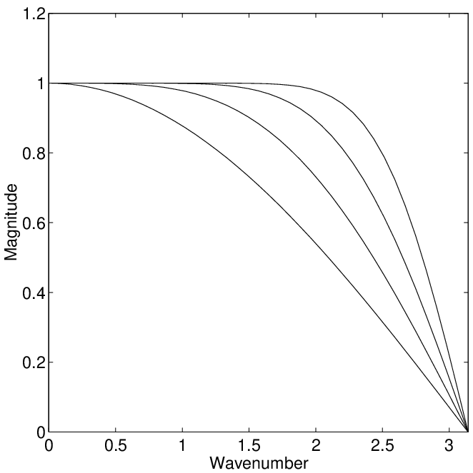
The feasibility of the DSC-RSK as lowpass filters in numerical computation is based on an important observation: by adjusting the ratio $r$ ($r=\frac{\sigma}{\Delta}$) of the regularizer, one can control the effective wavenumber region and thus, control the resolution of the lowpass filter. We plot the frequency response profile of the DSC-RSK lowpass filter in FIG. 1. A distinct property of the RSK lowpass filter is that there is no ripples in its passband; thus the application of this filter will not impart the low frequency. In contrast, some lowpass filters constructed with certain polynomials may have ripples in their passband, which would rule out their application to numerical integrations, especially for long time evolution, where the solution may be distorted after repeated filtering.

The maximum effective wavenumber (frequency) range of the DSC-RSK is determined by the ratio $r$, which in turn is determined by computational bandwidth $W$. The philosophy is simple since with the increase of $W$, the Gaussian window should also be enlarged to fully utilize the stencil. The optimal values $r$ at different $W$ can be estimated and they characterize the effective wavenumber range. The larger the optimal $r$ is, the wider the effective wavenumber range will be. When $r$ value is chosen larger than the optimal value for a given $W$, the accuracy of the resulting filter will be degraded by oscillations. Hence we do not recommend the use of $r$ beyond the optimal value unless in some circumstances where the filer is utilized to stabilize a long-time integration.

We denote $\zeta(x_{j})=\delta_{\sigma,\Delta}(x_{j})$ the proposed DSC-RSK lowpass filter in the physical domain $[0,L]$ and $\hat{\zeta}(\omega_{n})$ its image in the Fourier domain, where $\Delta=L/N$, $x_{j}=j\Delta$ and $\omega_{n}={2\pi n\over L}$. The obvious relation between $\zeta(x_{j})$ and $\hat{\zeta}(\omega_{n})$ is

$\displaystyle\hat{\zeta}(\omega_{n})=\Delta\sum_{j=0}^{N-1}{\zeta}(x_{j})e^{-i\omega_{n}x_{j}}.$

(8)

As in the previous work [15], filtering in the Fourier domain is usually accomplished by multiplying the given Fourier coefficients $\hat{u}(\omega_{n})=\Delta\sum_{j=0}^{N-1}{u}(x_{j})e^{-i\omega_{n}x_{j}}$ by $\hat{\zeta}(\omega_{n})$ directly, i.e., a windowed Fourier transform,

$\displaystyle u^{\zeta}(x_{j})={1\over L}\sum_{n=-{N\over 2}}^{{N\over 2}-1}\hat{\zeta}(\omega_{n})\hat{u}(\omega_{n})e^{i\omega_{n}x_{j}}.$

(9)

Therefore, the modified Fourier coefficients $\hat{\zeta}(\omega_{n})\hat{u}(\omega_{n})$ in Eq. (9) are the Fourier coefficients of a localized version of the original function $u(x_{j})$: $u^{\zeta}(x_{j})$. Hence, errors arising from the discontinuity are also localized and the accuracy away from the discontinuity can be ensured. In practical applications, one only needs to carry out the filtering and differentiation $D_{x}u=u_{x}$ in one step

$\displaystyle u_{x}^{\zeta}(x_{j})={1\over L}\sum_{n=-{N\over 2}}^{{N\over 2}-1}i\omega_{n}\hat{\zeta}(\omega_{n})\hat{u}(\omega_{n})e^{i\omega_{n}x_{j}}.$

(10)

A standard forth-order Runge-Kutta (RK-4) scheme is employed for the time advance scheme in this work. We use a TVD switch to adaptively activate the application of the DSC-RSK lowpass filter. Whenever the total variation of the approximate solution in the two consecutive time steps exceeds a prescribed criteria, the lowpass filter is activated. The DSC-RSK lowpass filter is only applied at the end of each full RK-4 cycle. The reader is referred to our earlier work [19, 45, 46] for the detail of this adaptive filtering.

It is more difficult to apply the filter in the physical domain than in the Fourier domain. On one hand, it is not easy to quantitatively analyze the influence of numerical dissipation in the physical domain. On the other hand, the convolution operation

$\displaystyle u^{\zeta}(x)=\int u(x-\xi)\zeta(\xi)d\xi,$

(11)

complicates the physical domain application of the filter. However, in some practical applications, it turns out to be quite necessary to implement the filter in the physical domain, especially for problems whose boundaries require some special treatments. The reflective boundary is one of such examples that need to be treated by using grid points outside the computational domain. In this work, we propose the method to apply our DSC-RSK lowpass filter in the physical domain. Due to the fact that the RSK lowpass filter is an interpolatory kernel, we consider a two-step procedure. Step one is the prediction of mid-mesh values from the nodal values

$\displaystyle u^{\zeta}_{i+\frac{1}{2}}=\sum^{-1}_{j=-W}u_{i+j+1}\zeta((j+\frac{1}{2})\Delta)+\sum^{W}_{j=1}u_{i+j}\zeta((j-\frac{1}{2})\Delta).$

(12)

The other is the reconstruction of the nodal values from the mid-mesh values

$\displaystyle u^{\zeta\zeta}_{i}=\sum^{-1}_{j=-W}u^{\zeta}_{i+j+\frac{1}{2}}\zeta((j+\frac{1}{2})\Delta)+\sum^{W}_{j=1}u^{\zeta}_{i+j-\frac{1}{2}}\zeta((j-\frac{1}{2})\Delta),$

(13)

where, $u_{i}$ denotes $u(x_{i})$ and $\Delta$ is the grid spacing. The lowpass filter with a $r$ value smaller than the optimal value is used in one of these two steps. The activation of the RSK lowpass filter is controlled in the same manner as that of the frequency domain algorithm.

As described, the DSC-RSK lowpass filter can be applied either in the physical domain or in the Fourier domain. In general, filtering in the Fourier domain is much easier and more convenient than in the physical domain because no additional summation is required to implement the filter in the Fourier spectral method. In contrast, the physical domain implementation requires two additional summations. Therefore, we have used the filter in the Fourier domain in most of our numerical experiments except for the cases in which the reflective boundary condition is involved. We have checked that whenever applicable, results obtained from the Fourier domain approach and the physical domain approach are identical.

Once the time integration has been completed, a strong filter is usually required for post processing the solution so as to make the solution more presentable. In principle, we only need to reduce the $r$ value of the DSC-RSK lowpass filter at the last time step of the computation. As an alternative, we provide a series of lowpass filters based on the Lagrange delta kernel which is given by

$\displaystyle\delta_{W}(x,x_{j})=\prod_{k=-W,k\neq j}^{W}\frac{x-x_{k}}{x_{j}-x_{k}},~~~~j=-W,\cdots,W.$

(14)

FIG. 2 shows the magnitude response of the Lagrange delta kernel. In fact, the highpass versions of these filters are graphically identical to centered finite difference (FD) schemes. In our numerical experiments, we adopt Lagrange-2 or Lagrange-4 as post processing filters. Their efficiency is demonstrated by our numerical results.

We begin our numerical experiments with the scalar conservation law system, which is given by

$\displaystyle u_{t}+f(u)_{x}=0,$

(15)

where $f(u)$ is a function of $u$. It is generally believed that spectral methods are not very suitable for simple shock profiles and should not be used if one is interested primarily in the shock profiles rather than other detailed structures of the flow. In this study, we choose scalar conservation law systems to illustrate that the proposed global spectral scheme performs well for a class of localized shock problems.

Example 1. We first solve a linear advection equation, which is of the form

$\displaystyle\begin{array}[]{rl}u_{t}+u_{x}=&0\quad-1<x<1,\\ u(x,0)=&u_{0}(x)\quad\text{periodic,}\end{array}$

where, $u_{0}$ is an initial value

$\displaystyle u_{0}(x)=\left\{\begin{array}[]{ll}\frac{1}{6}(G(x,\beta,z-\delta)+G(x,\beta,z+\delta)+4G(x,\beta,z))&\quad-0.8\leq x\leq-0.6\\ 1&\quad-0.4\leq x\leq-0.2\\ 1-|10(x-0.1)|&\quad 0\leq x\leq 0.2\\ \frac{1}{6}(F(x,\alpha,a-\delta)+F(x,\alpha,a+\delta)+4F(x,\alpha,a))&\quad 0.4\leq x\leq 0.6\\ 0&\quad\text{otherwise}.\end{array}\right.$

Here, functions $G$ and $F$ are defined as

$\displaystyle\begin{array}[]{rl}G(x,\beta,z)=&e^{-\beta(x-z)^{2}}\\ F(x,\alpha,a)=&\sqrt{\mbox{max}(1-\alpha^{2}(x-a)^{2},0)},\end{array}$

where $a=0.5$, $z=-0.7$, $\delta=0.005$, $\alpha=10$ and $\beta=\frac{\text{log}2}{36\delta^{2}}.$

The solution of this problem contains a combination of a Gaussian, a square wave, a sharp triangle wave and a half ellipse. The exact solution at any time can be easily obtained by a translation of the initial solution at speed 1. In FIG. 3 and FIG. 4, we display the numerical results for this problem at $t$=8 with 128 and 256 grid points, respectively. We observe that our method works well in both cases.

Example 2. Secondly, we test the proposed method by considering a moving W-shape wave, i.e., a piecewise continuous initial value, for the linear advection equation with an initial value [45]

$\displaystyle u_{0}(x)=\left\{\begin{array}[]{ll}1&\quad 0\leq x\leq 0.2\\ 4x-\frac{3}{5}&\quad 0.2\leq x\leq 0.4\\ -4x+\frac{13}{5}&\quad 0.4\leq x\leq 0.6\\ 1&\quad 0.6\leq x\leq 0.8\\ 0&\quad\text{otherwise}.\end{array}\right.$

This case is very similar to Example 1. It contains the so-called contact discontinuity and is quite difficult to solve in hyperbolic conservation laws. In particular, the interaction of two lines at $x=0.2$ and $x=0.6$ is difficult to resolve. Hence, it is a good test for the shock-capturing ability of the present method. We compute the solution up to $t$=8. The results are shown in FIG. 5 and FIG. 6.

Example 3. Having solved the linear equation with different initial values, we consider the solution of the most popular inviscid Burgers’ equation, in which $f(u)=u^{2}/2$ and the Riemann type initial value is given by

$\displaystyle u(x,0)=\left\{\begin{array}[]{ll}1&\quad x\leq 0\\ 0&\quad x>0.\end{array}\right.$

This is a standard benchmark problem in hyperbolic conservation laws and has been considered by numerous researchers. The exact solution is a shock wave with a constant velocity

$\displaystyle u(x,t)=\left\{\begin{array}[]{ll}1&\quad x-St<0\\ 0&\quad x-St>0,\end{array}\right.$

where the speed of the shock front is

$\displaystyle S=\frac{1}{2}.$

(40)

We should note that this case is a non-periodic boundary problem. We must symmetrically double the computational domain in the $x$-direction when we calculate the derivative of the flux. This operation is necessary because it generates the periodic boundary condition so that the Fourier spectral method can be used. The numerical results are plotted in FIG. 7 at time $t$=2.

Example 4. Another Riemann type initial value for the inviscid Burgers’ equation with a flux of $u^{2}/2$ is given by

$\displaystyle u(x,0)=\left\{\begin{array}[]{ll}0&\quad x<0\\ 1&\quad x\geq 0.\end{array}\right.$

The exact solution of this problem is a rarefaction wave

$\displaystyle u(x,t)=\left\{\begin{array}[]{ll}0&\quad\frac{x}{t}<0\\ \frac{x}{t}&\quad 0<\frac{x}{t}<1\\ 1&\quad\frac{x}{t}>1.\end{array}\right.$

Numerical results are plotted in FIG. 8 at $t$=2 with different numbers of nodal points. Particularly, one can see that the end of the rarefaction fan is well resolved.

Example 5. Finally, we use non-convex flux to test the convergence to the physically correct solution. The flux is a non-convex function

$\displaystyle f(u)=\frac{1}{4}(u^{2}-1)(u^{2}-4)$

(48)

with a Riemann type initial value

$\displaystyle u(x,0)=\left\{\begin{array}[]{ll}-3&\quad x<0\\ 3&\quad x\geq 0.\end{array}\right.$

The reader is referred to [20] for more detailed information about this problem. The results are displayed in FIG. 9 at $t$=0.04. Again, present spectral solver yields a satisfactory resolution.

In this subsection, we perform numerical experiments by using the proposed scheme for the 1D Euler equation of gas dynamics. In one dimension, the Euler equation takes the form

$\displaystyle U_{t}+F(U)_{x}=0$

(52)

with

$\displaystyle U=\left(\begin{array}[]{c}\rho\\ \rho u\\ E\\ \end{array}\right);\quad F(U)=\left(\begin{array}[]{c}\rho u\\ \rho u^{2}+p\\ u(E+p)\\ \end{array}\right),$

where, $\rho,u,p$ and $E$ denote the density, velocity, pressure and total energy per unit mass $E=\rho(e+(u^{2})/2)$, respectively. Here, $e$ is the specific internal energy. For an ideal gas with the constant specific heat ratio ($\gamma=1.4$) considered here, one has $e=p/(\gamma-1)\rho$. We consider the following two well-known Riemann problems.

Example 6. We solve for the solution of two shock tube problems with Sod’s and Lax’s initial conditions [23], i.e.,

$\displaystyle(\rho,u,p)_{t=0}=\left\{\begin{array}[]{ll}(1,0,1),&\quad x<0\\ (0.125,0,0.1),&\quad\text{otherwise}\end{array}\right.$

for the Sod problem and

$\displaystyle(\rho,u,p)_{t=0}=\left\{\begin{array}[]{lll}(0.445,0.698,3.528),&\quad x<0\\ (0.5,0,0.571),&\quad\text{otherwise}\end{array}\right.$

for the Lax problem. The numerical results for these two problems are shown in FIG. 10 and FIG. 11, respectively. We can see that the present method gives a good resolution in both cases. Similar to all the methods depending on the numerical dissipation, the resolution for the linear degenerate contact discontinuity is slightly lower than that for the generic nonlinear shock wave. If combined with Harten’s artificial compression method, present spectral solver should have better resolution for the contact discontinuity.

Example 7. In this example, the interaction of an entropy wave of small amplitude with a Mach 3 right-moving shock in a one-dimensional flow is investigated. The computational domain is taken as $[0,9]$ and the flow field is initialized with

$\displaystyle(\rho,u,p)_{t=0}=\left\{\begin{array}[]{lccl}(3.85714,&2.629369,&10.33333)&\quad x\leq 0.5\\ (e^{-\epsilon\mbox{sin}(\kappa x)},&0,&1.0)&\quad x>0.5\\ \end{array}\right.$

where $\epsilon$ and $\kappa$ are the amplitude and the wave number of the entropy wave before the shock. This problem is significant due to its relevance to the interaction of shock-turbulence. Spectral methods, by nature of their high accuracy and negligible dispersive and dissipative errors, are ideally suited to the numerical study of turbulence and have already been widely applied. Here we would like to argue the feasibility of the present spectral method to the shock-turbulence interaction. In our test, we vary the wavenumber of the pre-shock wave while keeping its amplitude unchanged ($\epsilon=0.01$). As the wavenumber increases, the problem becomes more and more challenging because the amplified high-frequency entropy waves after the shock are always mixed with spurious oscillations. As the wavenumber increases, it is very difficult to distinguish the high-frequency waves from the spurious oscillations. A low-order scheme may dramatically damp the transmitted high frequency waves. Even some popular high-order schemes also encounter the difficulty in preserving the amplitudes of the entropy waves due to their excessive dissipation with a given mesh size. Therefore, a successful shock-capturing method should be able to eliminate Gibbs’ oscillation while capturing the shock and preserving the high-frequency entropy waves.

In our test, we let the shock move from $x=0.5$ to $x=8.5$. For the purpose of comparison with the previous results, we only give the results at the interval $[4.0,9.0]$. Also, in order to discharge the transient waves due to the non-numerical initial shock profile, we plot the length of the amplified entropy waves in the same manner as that in Ref. [23]. Furthermore, we must point out two nontrivial remarks for the following cases with different $\kappa$. One is that we have replotted the final results in a denser grid, otherwise the bounded strip will not be fully spanned due to the fact that no enough grid values locate near all the peaks /valleys of the wave. Another is that we have used a local filter in order to eliminate the oscillations near the shock when we present final results after the computation.

First, we consider $\kappa=13$. In this case, the computational domain is deployed with 513 grids points. Such a mesh is suitable for the Fourier spectral method. The numerical results of the amplitude of the entropy waves are shown in FIG. 12(a). It can be seen that the shock and the generated entropy waves are ideally captured. The entropy waves fully span the strip bounded by two solid lines at $\pm$ 0.08690716, which show the amplitude of the amplified entropy waves predicted by the linear analysis. Since post-shock waves are monochromic, a simple calculation indicates the point per wavelength (PPW) value of these waves is 7.125. Such value is larger than the spectral resolution (PPW=2.0) but it is much smaller than that obtained by most shock-capturing schemes. The transmitted waves suffer the similar smearing as the contact waves. The shock wave, on the contrary, is self-repairable due to its compression nature. This observation verified that the numerical dissipation needed for shock-capturing will degrade the resolution of the spectral method. It also verified that this degradation can be isolated and alleviated by the DSC-RSK filter.

We next double the wave number $\kappa$ up to 26. A mesh of 513 grid points is not enough for simultaneous shock capturing and high-frequency wave resolving. Therefore, we increase the mesh size to $N=1025$ for this computation. The results for this case are presented in FIG. 12(b). It is seen that no obvious deterioration happens to the results and the resolution in the post-shock waves is still satisfactory. The fullness of the wave is comparable with that of $\kappa=13$. But the first two post-shock waves have been slightly polluted.

When the wave number $\kappa$ is increased to 39 and 52, we use 2049 grid points to resolve such high-frequency waves. FIG. 12(c) and FIG. 12(d) show the results of $\kappa=39$ and $\kappa=52$, respectively. The same PPW value $7.125$ is maintained in this high-frequency case. The good resolution of the present method in simulating this 1D shock entropy interaction indicates that our scheme is capable of and efficient in distinguishing the high-frequency entropy waves from spurious oscillations.

Example 8. Results are now shown for the problem of Shu and Osher which also describes the interaction of an entropy sine wave with a Mach 3 right-moving shock. The computational domain is taken as $[-1,1]$ and the flow field is initialized with

$\displaystyle(\rho,u,p)_{t=0}=\left\{\begin{array}[]{lcrr}(3.85714,&2.629369,&10.33333)&\quad x\leq-0.8\\ (1.0+\epsilon\mbox{sin}(\kappa\pi x),&0,&1.0)&\quad x>-0.8,\end{array}\right.$

where $\epsilon$=0.2 and $\kappa$=5. FIG. 13(a) and FIG. 13(b) show the solution of the density with 128 and 256 cells, respectively. The ‘Exact’ solution here is the solution computed by the third-order ENO with 1200 cells. As evident in the solution, the complicated flow field behind the shock is well resolved and the shock remains sharp. However, small oscillations near the shock still exist due to the fact that we do not attempt to locate this shock intentionally. If we predict the position of the shock and apply a local filter near the shock at the final time step, it is believed that more satisfactory results can be obtained.

In two dimensions, the Euler equation for gas dynamics in a vector notation takes the conservation form

$\displaystyle U_{t}+F(U)_{x}+G(U)_{y}=0$

(72)

with

$\displaystyle U=\left(\begin{array}[]{c}\rho\\ \rho u\\ \rho v\\ E\\ \end{array}\right);\quad F(U)=\left(\begin{array}[]{c}\rho u\\ \rho u^{2}+p\\ \rho uv\\ u(E+p)\\ \end{array}\right);\quad G(U)=\left(\begin{array}[]{c}\rho v\\ \rho uv\\ \rho v^{2}+p\\ v(E+p)\\ \end{array}\right),$

$\displaystyle p=(\gamma-1)(E-\frac{1}{2}\rho(u^{2}+v^{2})),$

(86)

where $(u,v)$ is the 2D fluid velocity and $\gamma=1.4$ is used in all computations.

Example 9. As the first example, we use our spectral scheme to study the interaction between a normal shock and a weak entropy wave which makes an angle $\theta\in(0,\pi/2)$ against the $x$-axis. If $\theta=0$, we have essentially the 1D problem (see example 7). The initial conditions are defined as follows: the right state of the shock is given as $(\rho_{r},u_{r},v_{r},p_{r})$=(1, 0, 0, 1) with a given shock Mach number $M_{s}=3$. We add a small entropy wave to the flow on the right of the shock which is equivalent to changing only the density of the flow on the right of the shock. In our problem we change the density $\rho_{r}$ in the right state of the shock by multiplying $\rho_{\epsilon}$

$\displaystyle\begin{array}[]{ll}\rho=&\rho_{r}\rho_{\epsilon}\\ \rho_{\epsilon}=&e^{-(\epsilon/p_{r})\sin(\kappa(x\cos\theta+y\sin\theta))}\end{array}$

with $\epsilon$ and $\kappa$ being the amplitude and wavenumber, respectively. In order to carry out a long time integration and to enforce periodic boundary condition in $y$-direction, the computational domain is taken to be $[0,9]\times[0,\frac{2\pi}{\kappa\sin\theta}]$. We initially position the normal shock at $x=0.5$ and allow it to move up to $x=8.5$. In our simulation, we adopt $\epsilon=0.1$, $\kappa=15$, and $\theta=30^{\circ}$. The performance is measured by drawing the maximum amplitudes of the amplified entropy waves in the $y$-direction for all fixed grid values $x\in[7.4,8.4]$, and comparing them with the amplitude predicted by the linear analysis, which is 0.08744786.

We use 513 grid points in the $x$-direction and 32 grid points in the $y$-direction in our test. In order to avoid peak/valley losses of the entropy waves due to insufficient grid points near these positions, we interpolate our final results to a denser grid when plotting them. FIG. 14 displays the amplitudes of the amplified entropy waves. Obviously, the compressed entropy waves are well resolved in the post-shock regime even though small oscillations remain near the location of the shock. It is believed that such a trivial flaw is acceptable.

This example has further demonstrated the capability of our spectral scheme for capturing small scale waves in the presence of a shock.

Example 10. This model problem describes the interaction between a stationary shock and a vortex. It has many potential applications and has been treated by many researchers using various techniques. Early numerical studies in this area using spectral methods focused primarily on shock-fitting techniques. However, for the cases in which a vortex causes a shock to deform at the point of bifurcation, it is generally difficult for a shock-fitting method to apply. This problem was successfully simulated in Refs. [6, 8] by using the Chebyshev spectral method. In this paper, we also adopt this model to access the capability of the proposed spectral shock-capturing method. This problem is defined as follows. The initialization is imposed on the domain $[0,2]\times[0,1]$ with a stationary normal shock at $x=0.5$ and a Mach 1.1 flow at the inlet. The right state of the shock is given as $(\rho_{r},u_{r},v_{r},p_{r})=(1,1.1\sqrt{\gamma},0,1)$. A vortex is generated by a perturbation to the velocity $(u,v)$, temperature $T$ and entropy $S$ which is centered at $(x_{c},y_{c})=(0.25,0.5)$ and in the forms

	$\displaystyle u^{\prime}$	$\displaystyle=$	$\displaystyle\epsilon\tau e^{\alpha(1-\tau^{2})}\sin\theta$		(90)
	$\displaystyle v^{\prime}$	$\displaystyle=$	$\displaystyle-\epsilon\tau e^{\alpha(1-\tau^{2})}\cos\theta$		(91)
	$\displaystyle T^{\prime}$	$\displaystyle=$	$\displaystyle-\frac{(\gamma-1)\epsilon^{2}e^{2\alpha(1-\tau^{2})}}{4\alpha\gamma}$		(92)
	$\displaystyle S^{\prime}$	$\displaystyle=$	$\displaystyle 0$		(93)

where, $\tau=\frac{r}{r_{c}}$, $r=\sqrt{(x-x_{c})^{2}+(y-y_{c})^{2}}$ and $\theta=\mbox{tan}^{-1}((y-y_{c})/(x-x_{c}))$. Here $\epsilon$ denotes the strength of the vortex, $\alpha$ is the decay rate of the vortex. Note that we can obtain perturbations in $\rho$ and $p$ according to the relations of $T=p/\rho$ and $S={\rm ln}\frac{p}{\rho^{\gamma}}$. In our numerical experiment, we choose $\epsilon=0.3$, $r_{c}=0.05$ and $\alpha=0.204$.

A reflective boundary is imposed on both the upper and lower boundaries. We solve the Euler equations on a 257 $\times$ 129 Cartesian grid, which is uniform in $y$-direction and refined in $x$-direction around the shock using the Roberts transformation [2]. Once again, we emphasize that the DSC-RSK lowpass filter is used in the physical domain directly for this problem due to the presence of the reflective boundaries. FIGs. 15(a-e) show a time evolution of shock-vortex interaction in terms of the pressure contours. We can see that even at $t$=0.8 the solution (FIG. 15(e)) is almost free of oscillations and the fine scale features are captured very well. Particularly, the shock bifurcation reflected on the top boundary is shown clearly.

In order to explore the potential of our algorithm further, we increase the flow Mach number up to 3.0 and the strength of the vortex $\epsilon$ up to 0.6. The results at $t$=0.2 are shown in FIG. 16. Deformation and bifurcation of the shock are observed clearly. These results indicate that the applicability of our spectral shock-capturing scheme is not limited to low Mach number and low vortex strength. Flows of high Mach number and high vortex strength can also be successfully simulated.

Example 11. In this case, we investigate the advection of an isentropic vortex in a free stream. As the exact solution of this problem is available, it is a good test for examining the accuracy and stability of shock capturing schemes.

Consider a mean flow of $(\rho_{\infty},u_{\infty},v_{\infty},p_{\infty},T_{\infty})=(1,1,1,1,1)$ with a periodic boundary condition in both directions. At $t_{0}$, the flow is perturbed by an isentropic vortex $(u^{\prime},v^{\prime},T^{\prime})$ centered at $(x_{0},y_{0})$, having the forms of

	$\displaystyle u^{\prime}$	$\displaystyle=$	$\displaystyle-\frac{\lambda}{2\pi}(y-y_{0})e^{\eta(1-s^{2})},$		(94)
	$\displaystyle v^{\prime}$	$\displaystyle=$	$\displaystyle~~\frac{\lambda}{2\pi}(x-x_{0})e^{\eta(1-s^{2})},$		(95)
	$\displaystyle T^{\prime}$	$\displaystyle=$	$\displaystyle-\frac{(\gamma-1)\lambda^{2}}{16\eta\gamma\pi^{2}}e^{2\eta(1-s^{2})}.$		(96)

Here, $s=\sqrt{(x-x_{0})^{2}+(y-y_{0})^{2}}$ is the distance to the vortex center; $\lambda$ is the strength of the vortex and $\eta$ is a parameter determining the gradient of the solution. In our test, we choose them as $\lambda=5$ and $\eta=1$ unless we further specify. Note that for an isentropic flow, relations $p=\rho^{\gamma}$ and $T=p/\rho$ are valid. Therefore, the perturbed $\rho$ is required to be

$\displaystyle\rho=(T_{\infty}+T^{\prime})^{1/(\gamma-1)}=\left[1-\frac{(\gamma-1)\lambda^{2}}{16\eta\gamma\pi^{2}}e^{2\eta(1-s^{2})}\right]^{1/(\gamma-1)}.$

(97)

The computational domain is taken to be $[0,10]\times[0,10]$ with the center of the vortex being initially located at $(x_{0},y_{0})=(5,5)$, the geometrical center of the computational domain.

Since there is no presence of shock in this problem, spectral method on its own can already provide excellent results if the time integration period is small enough. As such, the lowpass filter is not needed in an initial time period. However, as time progresses, errors would accumulate rapidly and the computation could become unstable if the lowpass filter is not activated to efficiently control the dramatically nonlinear growth of the errors. In our numerical experiment which is not shown here, the computation blows up at around $t$=13 if no filter is used.

Two experiments are conducted in this study. One is to examine the accuracy of our spectral code and the other is to investigate the stability of our scheme for a long time integration. For the first experiment, we compute the solution of $\rho$ at the time $t$=2 using three sets of meshes ($N=32,64,128$). To make the spatial error dominant, we optimize the CFL number to be 0.01.

Two error measures, $L_{1}$ and $L_{2}$, have been used. To be consistent with the literature [11], two errors used in this problem are defined as

	$\displaystyle L_{1}$	$\displaystyle=$	$\displaystyle{1\over(N+1)^{2}}\sum_{i=0}^{N}\sum_{j=0}^{N}|f_{i,j}-\bar{f}_{i,j}|$		(98)
	$\displaystyle L_{2}$	$\displaystyle=$	$\displaystyle{1\over(N+1)}\sqrt{\sum_{i=0}^{N}\sum_{j=0}^{N}|f_{i,j}-\bar{f}_{i,j}|^{2}},$		(99)

where $f$ is the numerical result and $\bar{f}$ the exact solution. Note that they are not the standard definitions. The errors for the density with respect to the exact solution are listed in Table I in which we also list the results of some other schemes for a comparison. As the table highlights, the accuracy of the Fourier spectral method is comparative to that of the DSC method [48], while both Fourier spectral and DSC methods are much more accurate than the fourth-order accurate, conservative central scheme (C4).

Our next numerical experiment concerns the performance of our spectral code for a long time integration. Here, we compute the solution of $\rho$ at the time $t$=100, 200, 400, 600, 800 and 1000, with the grid $N=64$. Note that we choose the gradient of the solution $\eta=0.5$ in this case. We list the $L_{1}$ and $L_{2}$ errors for the density in Table II. It can be seen that our spectral code is highly accurate even after such a long time evolution. The results indicate that our spectral scheme together with the DSC lowpass filter is reliable for the numerical approximation of conservation laws.

Example 12. Finally, we consider the problem of a supersonic flow past a cylinder [23]. This example is used to mainly examine the ability of our DSC filter spectral scheme in handling a non-rectangular domain.

The physical domain is on the $x-y$ plane, and the computational domain is chosen to be [0, 1] $\times$ [0, 1] on the $\xi-\eta$ plane. The mapping between the computational domain and the physical domain is

$\displaystyle\begin{array}[]{lr}x=&-(R_{x}-(R_{x}-1)\xi)\mbox{cos}(\theta(2\eta-1))\\ y=&(R_{y}-(R_{y}-1)\xi)\mbox{sin}(\theta(2\eta-1))\end{array}$

where we take $R_{x}=3$, $R_{y}=6$ and $\theta=\frac{5\pi}{12}$.

The flow field is initialized with a Mach 3 shock moving from the inlet, i.e., $\xi=0$, toward the cylinder. The state in front of the shock is given as $(\rho_{r},u_{r},v_{r},p_{r})=(1.4,1.0,0,1.0)$. We impose a reflective boundary condition on the surface of the cylinder, i.e., $\xi=1$, and the outflow boundary condition at $\eta=0$ and $\eta=1$. In our simulation, a uniform mesh of $65\times 129$ in the computation domain is used. FIG. 17(a) depicts a diagram of the mesh (drawing every other grid line) in the physical domain. Like the case on a rectangular domain, we double the computational domain in both $\xi$ and $\eta$ directions when we approximate the first order derivative of the flux using the Fourier spectral method. The numerical result given in terms of pressure contours (obtained at $t$=4.5) is shown in FIG. 17(b). In summary, our spectral scheme can be easily applied to the nonrectangular domain, as long as the domain can be smoothly transformed to the rectangular one.

References

- [1] S. Abarbanel, D. Gottlieb and E. Tadmor, Spectral methods for discontinuous problems, in Numerical Methods for Fluid Dynamics, (K. Morton and M. Baines eds.), (Oxford University Press, New York, 129-153 1986).
- [2] D. A. Anderson, J. C. Tannehill, and R. H. Pletcher, Computational fluid mechanics and heat transfer, (McGraw-Hill, New York, 1984).
- [3] F. Bianco, G. Puppo and G. Russo, High-order central differencing for hyperbolic conservation laws, SIAM J. Sci. Comput., 21, 294-322 (1999).
- [4] J. P. Boyd, Chebyshev and Fourier Spectral Methods, (2nd ed. Dover, New York, 2000).
- [5] W. Cai, D. Gottlieb and C.-W. Shu, Essentially nonoscillatory spectral Fourier methods for shock wave calculations, Math. Comp., 52, No. 186, 389-410 (1989).
- [6] W. Cai and C.-W. Shu, Uniform high-order spectral methods for one- and two-dimensional Euler equations, J. Comput. Phys., 104, 427-443 (1993).
- [7] C. Canuto, M. Y. Hussaini, A. Quarteroni and T. A. Zang, Spectral methods in fluid dynamics, (Springer-Verlag, Berlin, 1988).
- [8] W. S. Don, Numerical study of pseudospectral methods in shock wave applications, J. Comput. Phys, 110, 103-111 (1994).
- [9] W. S. Don and D. Gottlieb, Spectral simulation of supersonic reactive flows, SIAM J. Numer Anal., 35, 2370-2384 (1998).
- [10] B. Fornberg, A Practical Guide to Pseudospectral Methods, (Cambridge University Press, Cambridge 1996).
- [11] E. Garnier, P. Sagaut and M. Deville, A class of explicit ENO filters with application to unsteady flows, J. Comput. Phys., 170, 184-204 (2001).
- [12] D. Gottlieb, M. Y. Hussaini and S. A. Orszag, Introduction: Theory and Applications of Spectral Methods, in Spectral Methods for Partial Differential Equations, R. G. Voigt, D. Gottlieb and M. Y. Hussaini eds., (SIAM, Philadelphia, 1984).
- [13] D. Gottlieb and E. Tadmor, Recovering pointwise values of discontinuous data within spectral accuracy, in Progress and Supercomputing in Computational Fluid Dynamics, Earll M. Murman and Saul S. Abarbanel eds., (Birkh äuser, 357-375 1985).
- [14] D. Gottlieb, C.-W. Shu, A. Solomonoff and H. Vandeven, On the Gibbs phenomenon I, J. Comput. Appl. Math., 43, 81-98 (1992).
- [15] D. Gottlieb, Issues in the application of high order schemes, in Algorithmic Trends in Computational Fluid Dynamics, (Springer-Verlag, New York, 195-218 1993).
- [16] D. Gottlieb and C.-W. Shu, On the Gibbs phenomenon and its resolution, SIAM Review, 39, No. 4, 644-668 (1997).
- [17] D. Gottlieb and J. S. Hesthaven, Spectral methods for hyperbolic problems, J. Comput. Appl. Math., 128, 83-131 (2001).
- [18] T. Grahs and T. Sonar, Entropy-controlled artificial anisotropic diffusion for the numerical solution of conservation laws based on algorithms from image processing J. Vis. Commun. Image R., 13, 176-194 (2002).
- [19] Y. Gu and G. W. Wei, Conjugated filter approach for shock capturing, Commun. Numer. Meth. Engng., 19, 99-110 (2003).
- [20] A. Harten, B. Engquist, S. Osher and S. Chakravarthy, Uniform high-order accurate essentially non-oscillatory schemes, III, J. Comput. Phys., 131, 3-47 (1997).
- [21] J. S. Hesthaven and D. Gottlieb, Stable spectral methods for conservation laws on triangles with unstructured grids, Comput. Method Appl. Mech. Engng., 175, 361-381 (1999).
- [22] M. Y. Hussaini, D. A. Kopriva, M. D. Salas and T. A. Zang, Spectral methods for the Euler equation: Part I - Fourier methods and shock-capturing, AIAA J., 23, No. 1, 64-70 (1985).
- [23] G.-S. Jiang and C.-W. Shu, Efficient implementation of weighted ENO schemes, J. Comput. Phys, 126, 202 (1996).
- [24] S. Jin and C. D. Levermore, Numerical schemes for hyperbolic conservation laws with stiff relaxation terms, J. Comput. Phys., 126, 449-467 (1996).
- [25] A. Kurganov and D. Levy, A third-order semidiscrete central scheme for conservation laws and convention diffusion equations, SIAM J. Sci. Comput. 22, 1461-1488 (2000).
- [26] F. Lafon and S. Osher, Essentially nonoscillatory postprocessing filtering methods, in Algorithmic Trends in Computational Fluid Dynamics, (New York : Springer-Verlag, 219-243 1993).
- [27] F. Lafon and S. Osher, High order filtering methods for approximating hyperbolic systems of conservation laws, J. Comput. Phys., 172, 574-591 (1992).
- [28] R. J. LeVeque and M. Pelanti, A class of approximate Riemann solvers and their relation to relaxation schemes, J. Comput. Phys., 172, 574-591 (2001).
- [29] X.-D. Liu, S. Osher and T. Chan, Weighted essentially non-oscillatory schemes, J. Comput. Phys. 115, 200-212 (1994).
- [30] X.-D. Liu and E. Tadmor, Third order non-oscillatory central scheme for hyperbolic conservation laws, Numer. Math., 79, 397-425 (1998).
- [31] S. Lee, S. K. Lele and P. Moin, Interaction of isotropic turbulence with shock waves: Effect of shock strength, J. Fluid Mech., 340, 225-247 (1997).
- [32] A. Majda, J. McDonough and S. Osher, The Fourier method for nonsmooth initial data, Math. Comput., 32, No. 144, 1041-1081 (1978).
- [33] L. S. Mulholland and D. M. Sloan, The effect of filtering on the pseudospectral solution of evolutionary partial differential equation, J. Comput. Phys., 96, 369-390 (1991).
- [34] H. Nessyahu and E. Tadmor, Non-oscillation central differencing for hyperbolic conservation laws, J. Comput. Phys., 87, 408-463 (1990).
- [35] J.-X. Qiu and C.-W. Shu, On the construction, comparison, and local characteristic decomposition for high order central WENO schemes, J. Comput. Phys., in press.
- [36] C.-W. Shu, Essentially non-oscillatory and weighted essentially non-oscillatory schemes for hyperbolic conservation laws, ICASE Report, No. 97-65, (1997).
- [37] E. Tadmor, Convergence of spectral methods for nonlinear conservation laws, SIAM J. Numer. Anal., 26, 30-44 (1989).
- [38] E. F. Toro, R. C. Millington and V. A. Titarev, ADER: arbitrary-order non-oscillatory advection scheme, Proc. 8th International Conference on Non-linear Hyperbolic Problems, (Magdeburg, Germany, March, 2000).
- [39] L. N. Trefethen, Spectral Methods in Matlab, (Oxford University, Oxford, England, 2000).
- [40] H. Vandeven, Family of spectral filters for discontinuous problems, J. Sci. Comput., 6, 159-192 (1991).
- [41] D. C. Wan, B. S. V. Patnaik and G. W. Wei, Discrete singular convolution-finite subdomain method for the solution of incompressible viscous flows, J. Comput. Phys., 180, 229-255 (2002).
- [42] G. W. Wei, Discrete singular convolution for the solution of the Fokker-Planck equations, J. Chem. Phys., 110, 8930-8942 (1999).
- [43] G. W. Wei, Y. B. Zhao and Y. Xiang, Discrete singular convolution and its application to the analysis of plates with internal supports. I. Theory and algorithm, Int. J. Numer. Meth. Engng., 55, 913-946 (2002).
- [44] G. W. Wei, Oscillation reduction by anisotropic diffusions, Comput. Phys. Commun., 144, 317-342 (2002).
- [45] G. W. Wei, and Y. Gu, Conjugated filter approach for solving Burgers’ equation, J. Comput. Appl. Math., 149, 439-456 (2002); arXiv:math.SC/0009125, Sept. 13, (2000).
- [46] Y. C. Zhou and G. W. Wei, High resolution conjugate filters for the simulation of flows, preprinter.
- [47] K. Xu, A gas-kinetic BGK scheme for the Navier-Stokes equations and its connection with artificial dissipation and Godunov method, J. Comput. Phys., 171, 289-335 (2001).
- [48] S. Y. Yang, Y. C. Zhou, and G. W. Wei, Comparison of the discrete singular convolution algorithm and the Fourier pseudospectral method for solving partial differential equations, Comput. Phys. Commun., 143, 113-135 (2002).
- [49] H. C. Yee, N. D. Sandham and M. J. Djomehri, Low-dissipative high-order shock-capturing methods using characteristic-based filters, J. Comput. Phys. 150, 199-238 (1999).