Moduli of continuity and average decay of Fourier transforms: two-sided estimatesThe author was supported in part by NSF grant INT–0204308 U.S.–Sweden Collaborative Workshop on PDE’s and Spectral Theory, the Swedish foundation STINT grant PD2001–128 and NSF grant DMS–0550649. The author would like to thank the University of Pennsylvania and the Courant Institute for financial support and hospitality. The author is grateful to Percy Deift for his valuable suggestions which have helped to improve the presentation.
Abstract.
We study inequalities between general integral moduli of continuity of a function and the tail integral of its Fourier transform. We obtain, in particular, a refinement of a result due to D. B. H. Cline [2] (Theorem 1.1 below). We note that our approach does not use a regularly varying comparison function as in [2]. A corollary of Theorem 1.1 deals with the equivalence of the two-sided estimates on the modulus of continuity on one hand, and on the tail of the Fourier transform, on the other (Corollary 1.5). This corollary is applied in the proof of the violation of the so-called entropic area law for a critical system of free fermions in [4, 5].
Key words and phrases:
Modulus of continuity, Fourier transform2000 Mathematics Subject Classification
Primary: 42B10, 26B05. Secondary: 26D10.1. Introduction and statement of the main results
A result of this paper (Corollary 1.5 below) is applied in the proof of the violation of the so-called entropic area law for a critical system of free fermions, see [4, (6) et seq.], [4, Section on Fractal Boundaries] and [5, Lemma 2.10]. Corollary 1.5 follows from more general results of this paper (Theorems 1.1, 1.4) which are of independent interest.
It is well-known that the behavior of a modulus of continuity of a function for small is related to the behavior of the Fourier transform of for large (precise definitions are given in (1.3) et seq. below), see e.g. [10, Proposition 5.3.4], [12, Theorem 85]. The main object of our study are inequalities between general averaged moduli of continuity (m.c.) of functions (defined in (1.3) below) and tails of their Fourier transforms (F.t.). In [2] several results relevant for our purposes were obtained. Theorem 1.1 below gives a lower estimate for a general m.c., , in terms of the modified tail integral of the F.t. improving one of the results in [2] (as in [2], we distinguish between the true and the modified F.t. tail integral, as defined in (1.5) and (1.6) below). Corollary 1.2 gives a two-sided estimate for the m.c. in terms of the modified tail integral of the F.t. in the case . In applications it might be desirable to use the true F.t. tail instead of the modified tail that arises naturally in the mentioned inequalities. Theorem 1.4 gives the best possible power-scale description of the relationship between the true and the modified F.t. tails (see Remark 2.3).
Before stating our results we need to introduce some notation and recall two results in [2]. Let and denote by the standard norm in , . The Fourier transform , , of a function for is defined in the standard way (see e.g. [8, Section IV.3]). In the case we consider only the functions whose transforms belong to , . Introduce the difference operator of order acting on functions with domain by [11, Section 3.3]
| (1.1) |
where denotes the binomial coefficient. Note that the Fourier transform of (1.1) in equals and hence the functions
| (1.2) |
form a Fourier pair for . Now we define for any , , as the inverse Fourier transform of the second function in (1.2). Let denote the unit sphere in and let denote the standard measure on . (All the results below with obvious modifications hold if one replaces the standard measure on , with a measure invariant under orthogonal transformations and supported in the unit ball in as in [2].) For set
and define a general averaged (integral) m.c. of as follows. For any in the case set
| (1.3) |
(where in the case the integral should be interpreted as a sum over ), and in the case set
The Hölder inequality implies that for any there exists so that
| (1.4) |
Define the tail integral of the F.t. for and for , respectively, by
| (1.5) |
Motivated by the results in [2], we wish to compare the m.c. and the F.t. tail , as . It will be clear from our Theorem 1.1 below that the natural choice of for the purpose of such a comparison is (see also the discussion preceding Theorem 1.3). Note next that it is possible that is rapidly decreasing, or simply zero, for large (take e.g., ), whereas the modulus of continuity related to the th finite difference of vanishes generally speaking at the rate only. This motivated the author in [2] to introduce the following modified F.t. tails: For
| (1.6) | ||||
and for
It might not be immediately obvious why these tails are useful, we give the reason for that in Theorem 1.3 below. Note that for any , is nonincreasing as grows, because so is the function for any fixed . Note also that in the case , , there exist , such that
| (1.7) |
because for large .
We are ready to state the two results from [2] mentioned above. First [2, p. 512], for any in the case , there exists such that for for all functions in the set ,
| (1.8) |
Note that in the case , (1.8) holds for all . (The mentioned formula in [2] involves in fact . The formula (1.8) is then true since is nonincreasing, and (1.8) suffices for our purposes.) Secondly [2, (9)], for any in the case , for any there exists such that for any and for all
| (1.9) |
It would be preferable to have instead of (1.9) a formula which does not involve an infinite sum, i.e., of the type (1.8). It turns out that such a result holds for and if is large enough, at least .
Theorem 1.1
For any and there exists such that for all
| (1.10) |
It is explained in Remark 2.2 below why (1.10) (and even its analog with in the left-hand side, cf. (1.15) below) fails for . In view of (1.4), one can replace in the right-hand side in (1.10) with any (and a different ). It would be interesting to know if one could replace in the right-hand side of (1.10) with . Note also that for , our Theorem 1.1 implies readily all the statements of [2, Theorem 2], and is slightly more general since no comparison function as in [2] is required.
Corollary 1.2
For and there exist that depend on and only, such that for all and
| (1.11) | ||||
The estimates (1.8), (1.10), (1.11) show that that the modified F.t. tail is more appropriate than the true F.t. tail to be compared with the m.c. . The upper estimate in (1.11) is a Jackson-type inequality, see e.g. [8, Section I.8].
It follows from (1.11) that for an inequality in the direction opposite to (1.4) holds: In the case for all
| (1.12) |
and so for any all the moduli , , are equivalent. It would be interesting to find a direct proof of (1.12).
We now explain why in the case and the modified F.t. defined in (1.6) is a natural quantity to consider. For and any define
| (1.13) |
Recalling that the functions in (1.2) form a Fourier pair and using the Hausdorff–Young inequality (see the proof of Theorem 1.1 below and the proof of (1.8) in [2]) we can compare for fixed and , the norm of , , and the norm of the function (in the case we assume in addition as before that . Raising both quantities to the power (this explains why the choice is natural) we can compare the quantities and
With this in mind, for and any , , we introduce the Bessel tail of the Fourier transform
and . From the above discussion, can be compared with the Bessel tail as in (1.8), (1.10). The relevance of the modified F.t. is now apparent from the following
Theorem 1.3
For any and any , there exist that depend only on and so that
| (1.14) |
and hence for some that depend on , , only,
for all and all .
We now describe the relationship between the true and the modified F.t. tails, and , respectively. From (1.6) it is clear that for any , , and
| (1.15) |
The following statement gives a converse to (1.15) that is optimal on the power scale (see Remark 2.3 below).
Theorem 1.4
Let , , , , . All the constants below depend on and are strictly positive and finite.
1. Let .
(i) If , , then as ,
(ii) If , , then as ,
2. Let .
(i) If , , then as ,
(ii) If , , then as ,
We state finally a result that was applied in a study of the scaling of entanglement entropy for a certain physical system in [4, 5].
Corollary 1.5
Let . Assume that . Then for some , and some , satisfies
| (1.16) |
if and only if there exist , such that
| (1.17) |
Note that Corollary 1.5 is true in all dimensions: In the proof of Corollary 1.5 below, we consider the cases and separately. In the former case we employ the general results stated above. In the case we give a direct proof using in particular the ideas in the proofs of [1, Lemma 2.10, Lemma 4.2]. The main reason why, in the case , Corollary 1.5 is true despite the fact that Theorem 1.1 fails, is because of the explicit (power-type) form of the estimates in Corollary 1.5.
The equivalence of the upper estimates in (1.16) and in (1.17) is well-known: it follows follows e.g. from [9, Lemma 3.3.1], and also from the results obtained in [2]. Note that [9, Lemma 3.3.1] deals with a Besov space , , (the case is relevant for the upper estimates in Corollary 1.5). In [1], (1.17) is derived in the case from a more restrictive pointwise condition
| (1.18) |
which in general can not be reversed because can have singular directions.
A simple example of a function that satisfies (1.16) with is the characteristic function of a compact set with boundary. For any there exsits a compact set whose characteristic function satisfies (1.16), see [5, Lemma 2.9].
2. Proofs and concluding remarks
Proof of Theorem 1.1.
First consider the case , (in this case the proof below goes through for all ). We have to prove that for some , , . Recall that . Since the functions (1.2) form a Fourier pair we have
| (2.1) | ||||
It is an easy exercise to prove that for any
Consider now the case , , . By the Hausdorff–Young inequality , , and using the fact that (1.2) is a Fourier pair we get as in [2, (4.7)]
| (2.2) | ||||
Integrating over and recalling (1.13) we obtain
| (2.3) | ||||
Now we need the following elementary result, the proof is given after the end of the present proof.
Lemma 2.1
Let and fix any . The function , , defined in (1.13) satisfies the following: For any there exist such that
| (2.4) |
and
| (2.5) |
Remark 2.2.
We show now that (1.10) is not true in the case and . More precisely, we show that for there is no so that for all
| (2.7) |
By (1.2) with using the Parseval formula we find
| (2.8) |
For , , introduce the notation
where for , , , respectively, and . If (2.7) were true for some then there would exist such that
But
We have arrived at a contradiction: If
then we must have for a.e. and all , which is clearly false for any choice of . This proves the result.
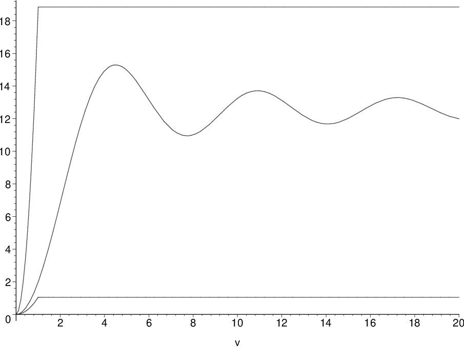
We note that the basic reason for the inapplicability of Theorem 1.1 to the case is that for any it is not possible to insert a constant function between the graph of and the real axis on the interval , cf. Fig. 1. (In the case , and so the function in (1.13) would be given by , , and there is no helpful averaging over .)
Proof of Lemma 2.1.
Recall that . If then integrating over the angles in (1.13) as in [3, (II.3.4.2)] we obtain for
| (2.9) |
If then (2.9) and the subsequent formlulae hold true with the convention .
We show first there is such that for sufficiently large . Indeed, in the case by the Hölder inequality there is so that
| (2.10) | ||||
where the second inequality follows from
| (2.11) |
with and . In the case , in view of (2.11) with and we obtain
| (2.12) | ||||
Note that
| (2.13) | ||||
where , is the Bessel function, and we have used [3, (II.3.4.2)] and [7, (8.411.4)]. By [7, (8.451)], , as for . Hence the right-hand side of (2.13), and also of (2.10) and (2.12), tends to a strictly positive limit, as . Therefore for any fixed , there exist and so that for .
But does not have zeros other than . Since is continuous, it is for any bounded away from zero on the compact . This proves (2.4).
Let us now prove (2.5) for small enough. We can rewrite (2.9) as
| (2.14) |
Using the elementary estimate
| (2.15) |
we conclude that
which proves (2.5) for any . But now if we take any then using (2.5) for and the fact that is bounded away from zero for by (2.4) we can always find small enough so that (2.5) holds for . The proof of Lemma 2.1 is complete. ∎
Proof of Theorem 1.3.
Recall that . The lower estimate in (1.14) follows immediately from Lemma 2.1 with . As for the upper estimate, we note first that by the definition (1.13), the function is bounded above for . Next, using the estimate , , in place of (2.15), we derive from (2.14) the upper estimate
This proves the upper estimate in (1.14). The proof of Theorem 1.3 is complete. ∎
Proof of Theorem 1.4.
Recall that , , .
1. Consider first the case .
(i) Assume , . By (1.6)
| (2.16) |
Then the following gives the result for the case 1(i), all values of :
where denotes the integer part of a real number. It is explained in Remark 2.3 below why the order in cannot be improved in the case 1(i) and in all other cases.
(ii) Assume , (). The example , , shows that in the case we can only claim the trivial bound , . Let now . We use the idea in the proof of [1, Lemma 4.2]. Let be a number to be chosen later. By the definition (2.16)
| (2.17) |
We have
Therefore choosing small enough (recall that ) we obtain that
| (2.18) |
Since , , (2.18) together with (2.17) gives
Setting we obtain
| (2.19) |
Noting that we conclude from (2.19) that
2. The case .
(i) Assume , . Note that
| (2.20) |
Clearly
| (2.21) |
Therefore
This together with (2.20) proves the case 2(i).
(ii) Let , . Again if then the example of , , shows that generally speaking only the trivial bound holds for large . Let now . Let be a number to be chosen later. We have
Now
Choosing small enough (note that ) we obtain
which implies that . Replacing we obtain
| (2.22) |
Noting that we conclude from (2.22) that
This completes the proof of Theorem 1.4. ∎
Remark 2.3.
Let us explain why the estimates in Theorem 1.4 have the best possible order in . In view of (1.15), the estimates 1(i) and 2(i) for can not be improved. The example of , , in view of the lower estimate in (1.7) shows that estimates 1(i) for and 1(ii), 2(i), 2(ii) for can not be improved. The example of , , such that for and smooth for shows that the estimate 1(ii) for can not be improved (note that the mentioned satisfies , , and also , ). Choosing such that for and smooth for shows that the estimate 2(ii) for can not be improved (for this we have , ). Finally, the example , , such that , , and smooth for shows that 1(i) for can not be improved. Indeed for this , , , but , .
Proof of Corollary 1.5.
The case . The result follows readily from Corollary 1.2 combined with Theorem 1.4 for , , , with . Note that the quantitity in the middle in (1.16) is . The integral in (1.17) is the true tail integral of the F.t. of , . By Corollary 1.2, the exist that depend on only so that for all
| (2.23) |
Set . Note that since we have , and the reult follows from Theorem 1.4, cases 1 (i) and (ii), applied to the comparison function , .
The case . We prove first that (1.16) implies (1.17). This follows from a straightforward modification of the proof of [1, Lemma 4.2]. We prefer to give the details for the convenience of the reader. Below, will denote a positive constant whose precise value may change from equation to equation and may depend on but which is independent of and . By (2.8)
Setting and denoting by again, we find from the upper inequality in (1.16)
which after setting implies
| (2.24) |
Using the latter estimate and representing
we prove the upper inequality in (1.17). In order to prove the lower inquality in (1.17), we note first that (2.24) implies
| (2.25) |
Indeed using the upper inequality in (1.17) we obtain
(recall that ). Next, let be two numbers to be chosen later. From the lower inequality in (1.16) and (2.8) using and for , we obtain
Using (2.25) and the upper inequality in (1.17) we find
which after choosing small enough and large enough gives
Setting we prove the lower inequality in (1.17).
We now derive (1.16) from (1.17). Using the upper inequality in (1.17) and employing (1.15) and Theorem 1.4 (recall that in our case , , )
Combining this with (1.8) (that holds for ) and using (1.4) we obtain
which proves the upper estimate in (1.16). It remains to prove the lower estimate in (1.16). Note that the two-sided estimate (1.17) implies that for large enough
or after setting
| (2.26) |
On the other hand again using (2.8)
and replacing with , , we find
Choosing we then obtain
where we have used (2.26). Therefore
and hence as is fixed, there exists at least one such that
Then
and denoting by we finish the proof of the lower inequality in (1.16). ∎
We note finally that the proof of Corollary 1.5 for can be modified to give an alternative proof of Corollary 1.5 also for all from scratch (in this connection, see an explanation of an argument from [1] given in the proof of [6, Lemma 3.4.1]).
Remark 2.4.
After the above general discussion it is not difficult to understand why Corollary 1.5 fails for . Recall that in (2.23), and . Let be defined by for and smooth for . Let be the inverse F.t. of this . It is easy to check that for some that depend on
| (2.27) |
whereas for certain that depend on
Note that by (2.23) and (2.27) for that depend on
This shows that Corollary 1.5 fails for . It is only true in the case that the upper estimate in (1.16) implies the upper estimate in (1.17) (simply because for any and all , in view of (1.15) and (1.10)). The fact that the lower estimate in (1.17) need not hold is shown by considering the example of , (for which identically for large ). Finally, the first example of this remark shows the upper estimate in (1.16) for need not follow even from a two-sided estimate in (1.17).
References
- [1] L. Brandolini, L. Colzani and G. Travaglini, Average decay of Fourier transforms and integer points in polyhedra. Ark. Mat. 35 (1997), 253–275.
- [2] D. B. H. Cline, Regularly varying rates of decrease for moduli of continuity and Fourier transforms of functions on . J. Math. Anal. Appl. 159 (1991), 507–519.
- [3] I. M. Gel’fand and G. E. Shilov, Generalized Functions, vol. 1, Academic Press, New York–London, 1964.
- [4] D. Gioev and I. Klich, Entanglement entropy of fermions in any dimension and the Widom conjecture. Phys. Rev. Lett. 96 (2006), 100503, 4 pp.
- [5] D. Gioev, Szegö limit theorem for operators with discontinuous symbols and applications to entanglement entropy. Int. Math. Res. Not. 2006, Art. ID 95181, 23 pp.
- [6] D. Gioev, Generalizations of Szegö Limit Theorem: Higher Order Terms and Discontinuous Symbols, Ph.D. Thesis, Royal Institute of Technology, Stockholm, 2001. www.math.rochester.edu/people/faculty/gioev/thesis.pdf
- [7] I. S. Gradshteyn and I. M. Ryzhik, Tables of Integrals, Series, and Products, 4th ed., Academic Press, New York–London–Toronto, 1980.
- [8] Y. Katznelson, An Introduction to Harmonic Analysis, 3rd Ed., Cambridge University Press, Cambridge, 2004.
- [9] V. G. Maz’ya and T. O. Shaposhnikova, Theory of Multipliers in Spaces of Differentiable Functions, Pitman Publishing, Boston, 1985.
- [10] E. Stein, Singular Integrals and Differentiability Properties of Functions, Princeton University Press, Princeton, 1970.
- [11] A. F. Timan, Theory of Approximation of Functions of a Real Variable, Pergamon Press, Oxford–New York, 1963.
- [12] E. C. Titchmarsh, Introduction to the Theory of Fourier Integrals, 2nd ed., Oxford University Press, London–New York, 1948.