Spectral triples from Mumford curves
Abstract
We construct spectral triples associated to Schottky–Mumford curves, in such a way that the local Euler factor can be recovered from the zeta functions of such spectral triples. We propose a way of extending this construction to the case where the curve is not -split degenerate.
1 Introduction
Let be a curve over a finite extension of , which is -split degenerate, for the residue field. It is well known that such curve admits a -adic uniformization by a -adic Schottky group acting on the Bruhat-Tits tree . We associate -algebras to certain subgraphs of the Bruhat-Tits tree and construct corresponding dynamical cohomologies that resemble the construction at arithmetic infinity given in [6]. We introduce a Dirac operator , which depends on the graded structure of the dynamical cohomology, in such a way that the data
give a spectral triple in the sense of Connes.
We recover, from a certain family of zeta functions associated to the spectral triple, the local Euler factor of the curve , in the form of a regularized determinant as computed by Deninger. The advantage of this construction is that it provides, in the case we are considering, a natural geometric interpretation, in terms of dynamics of walks on the graph , of the infinite dimensional cohomology theory introduced by Deninger.
We propose a way of extending the construction to the case where the curve is not -split degenerate, by enlarging the dual graph of the special fiber by new edges, in such a way that we also obtain embeddings in the dynamical cohomology of the first cohomology group of the components of the special fiber.
2 Directed graphs
We begin by recalling some generalities about graphs that we will use throughout the paper.
A directed graph consists of data , where is the set of vertices, is the set of oriented edges , where is an edge of the graph and is a choice of orientation. The set consists of a choice of orientation for each edge, namely one element in each pair . The maps are the range and source maps, and is the involution on defined by .
A morphism of directed graphs and consists of maps and which satisfy , , and , for . The morphism is a monomorphism if the are invertible, for . This defines the automorphism group of a directed graph, which we denote . A morphism of directed graphs is a covering map if the are onto, for , and gives a bijection and the same with respect to the range map.
A directed graph is finite if and are finite sets. It is row finite if at each vertex there are at most finitely many edges in such that . The graph is locally finite if each vertex emits and receives at most finitely many oriented edges in . A vertex in a directed graph is a sink if there is no edge in with source . We denote by the subset of given by the sinks.
A juxtaposition of oriented edges is said to be admissible if and . A (finite, infinite, doubly infinite) walk in a directed graph is an admissible (finite, infinite, doubly infinite) sequence of elements in . A (finite, infinite, doubly infinite) path in is a walk where all edges in the sequence are in . We denote by the set of walks of length , by , by the set of infinite walks, and by the set of doubly infinite walks. Similarly, we introduce the analogous notation , , and for paths. We shall drop the explicit mention of the graph in the notation for walks and paths, when no confusion arises. We denote by the set of paths that end at a sink. A directed graph is a directed tree if, for any two vertices, there exists a unique walk in connecting them.
The universal cover of a connected directed graph , endowed with a choice of a base point , is a directed tree obtained by setting , the set of all walks in that start at , , , , . The fundamental group of , with respect to the choice of base point , is given by .
Let be a subgroup of . We can then form the quotient , which is also a directed graph. In particular, if is the universal cover of a directed graph and is the fundamental group, with respect to the choice of a base point , then we have an isomorphism of directed graphs . The map is a covering map.
Two paths in are shift-tail equivalent, if there exists a and a such that for all . The boundary of a directed tree is given by , where the shift-tail equivalence is extended to the set of paths ending at a sink by the condition , for , if and only if . This definition extends to a functorial notion of boundary of directed graphs, as shown in [21].
3 Schottky-Mumford curves
Throughout this chapter we will denote by a fixed prime number and by the field of -adic numbers. The field will be a given finite extension of , with its ring of integers, the maximal ideal and a uniformizer (i.e. ). Finally, we will denote by the residue field . This is a finite field of cardinality .
Let be a two-dimensional vector space over . We write for the set of -rational points of , the projective line over . The space is identified with the set of -lines passing through the origin in . Let be the group of automorphisms of .
In this first chapter we collect some well known facts and properties on the tree of the group and on the action of a Schottky group on such tree. Detailed explanations for the statements we will recall here without proofs are contained in [14] and [18].
3.1 The tree of the group PGL(2,K)
The description of the vertices of the tree associated to is as follows. One considers the set of free -modules of rank : . Two such modules are equivalent if there exists an element , such that . The group of linear automorphisms of operates on the set of such modules on the left: , . Notice that the relation is equivalent to the condition that and belong to the same orbit of the center . Hence, the group operates (on the left) on the set of classes of equivalent modules.
We denote by the set of such classes and by the class of the module . Because is a principal ideals domain and every module has two generators, it follows that
The multiplication of and by elements of preserves the inclusion , hence the natural number
| (3.1) |
is well defined.
Definition 3.1
The graph of the group is the infinite graph with set of vertices , in which two vertices are adjacent and hence connected by an edge if and only if .
Proposition 3.2
- 1.
The graph is a connected, locally finite tree with edges departing from each of its vertices.
- 2.
The shortest walk in connecting two vertices of without back-tracking has length .
- 3.
The group acts (on the left) transitively on and it preserves the metric .
The tree is called the Bruhat–Tits tree associated to the group .
A half-line in is an infinite sequence of vertices of without repetitions such that is adjacent to for all . Thus, a half-line is given by a sequence of free -modules where for all .
The subspace defines a point of . Conversely, given a point of represented by a vector , choose a second vector such that form a basis of . Let be the free -module with basis . Then, defines the point of we started with.
Two half-lines are said to be equivalent if they differ only by a finite number of vertices. An equivalence class of halflines is called an end of . The set of ends of will be denoted by (the “boundary” of ). We shall give the structure of a directed graph, in such a way that this notion of boundary agrees with the one described in the previous section.
It is immediate to verify that the construction described above defines a one-to-one correspondence between equivalence classes of half-lines and elements of .
3.2 The action of a Schottky group on the tree
A Schottky group is a subgroup of which is finitely generated and whose elements are hyperbolic (i.e. the eigenvalues of in have different valuation). The group is discrete in , torsion free and acts freely on the tree . Furthermore, one can show that acts discretely at some point .
Let be the closure of the set of points in that are fixed points of some . This is called the limit set of . We have if and only if , for some . We will denote by the set of points on which acts discretely; equivalently said is the set of points which are not limits of fixed points of elements of : . This set is called the domain of discontinuity for the Schottky group .
A path in , infinite in both directions and with no back-tracking, is called an axis of . Any two points uniquely define their connecting axis whose endpoints lie in the classes described by and in .
Any hyperbolic element has two fixed points in . The unique axis of whose ends are fixed by is called the axis of . The element acts on its axis as a translation.
Suppose two axes are given in . Any path without back-tracking beginning on one axis and ending on the other and with no edges in common with either axis is said to be the bridge between them. A bridge may consist of a single point, else it is uniquely defined (Figure 1).

For any Schottky group there is a smallest subtree containing the axes of all elements of . Equivalently said, is the maximal connected subgraph of containing the axes of all elements of and the bridges between them.
The set of ends of in is , the limit set of . The group carries into itself so that the quotient is a finite graph.
The graph has an important geometric interpretation as the dual graph of the closed fiber of the minimal smooth model over (-split degenerate semi-stable curve) of the algebraic curve holomorphically isomorphic to (cf. [18] p. 163).
Furthermore, there is a smallest tree on which acts, with vertices , and such that the finite graph is the dual graph of the specialization of over . The set is a subset of the set of vertices of .
The degenerating curve describing the analytic uniformization is a -split degenerate, stable curve. When the genus of the fibers is at least 2 - i.e. when the Schottky group has at least generators - the curves are called Schottky–Mumford curves.
3.3 Field extensions: functoriality
Let be a finite fields extension with ramification index and rings of integers and . If is a free -module of rank , then is a free -module of the same rank. It is obvious that equivalent modules remain equivalent, hence one gets a natural embedding of the sets of vertices .
The isomorphism shows that distance would not, in general, be preserved under field extensions. To eliminate this disadvantage, one introduces on graphs , for all extensions , a -normalized distance
This way, the embedding becomes isometric. When ramifies, new vertices appear in between each couple of adjacent vertices in (cf. the third graph in Figure 2). Moreover, edges each of which of length , for , depart from each vertex in (cf. the second graph in Figure 2).
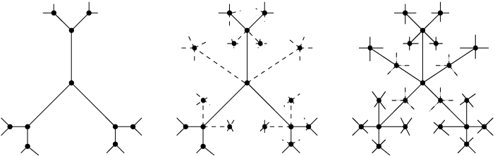
Because and the natural embedding is compatible with a concept of -direction of exiting from any vertex of , the construction is functorial under finite fields extensions and this process determines, for a fixed Schottky group , a projective system of Schottky-Mumford curves.
3.4 Edge orientation
We now show how to endow the graphs and with the structure of directed graph. The choice of a coordinate determines a base point in . In fact, the points on determine a unique crossroad: the unique vertex of with the property that the walks without back-tracking from to the three points on start from in three different directions (Figure 3).

In order to obtain a structure of directed graph on the tree , for each we consider the unique infinite chain of edges without backtracking in that has initial vertex and whose equivalence class modulo shift–tail equivalence is the point . We declare such chain of edges to be a path in . This determines on the structure of a directed graph, with . This agrees with the boundary as defined in §3.1.
We assume here that the coordinate is chosen in such a way that the crossroad of is a vertex of . Then, by the same procedure, we can regard as a directed graph with .
4 -algebras of graphs
In this section we recall the construction of -algebras associated to locally finite directed graphs. We follow mostly the references [1], [10], [11], [21]. We refer the reader to the bibliography of the aforementioned articles for more information. For simplicity, we state the following results in the special case of locally finite directed graph, though the theory extends to more general directed graphs (cf. e.g. [21]).
A Cuntz–Krieger family consists of a collection of mutually orthogonal projections and of partial isometries, satisfying the conditions: and, for all , .
The edge matrix of a locally finite (or row finite) directed graph is an (possibly infinite) matrix. The entries satisfy if is an admissible path, and otherwise. The Cuntz–Krieger elements satisfy the relation . The directed edge matrix of is a (possibly infinite) matrix with entries if is an admissible walk and otherwise.
There is a universal -algebra generated by a Cuntz–Krieger family. If is a finite graph with no sinks, we have , where is the Cuntz-Krieger algebra of the edge matrix . If the directed graph is a tree , then is an AF algebra strongly Morita equivalent to the commutative -algebra . A monomorphism of directed trees induces an injective -homomorphism of the corresponding -algebras.
If is a group acting freely on the directed graph , with quotient graph , then the crossed product -algebra is strongly Morita equivalent to . In particular, if is the universal covering tree of a directed graph and is the fundamental group, then the algebra is strongly Morita equivalent to .
There is a gauge action of on the graph algebra given by . A subset of the set of vertices of a directed graph is saturated hereditary if implies that, for all with , also , and conversely, if any with satisfies , then also . For a locally finite graph there is a bijective correspondence between saturated hereditary subsets of and gauge invariant closed ideals in . In the case of a tree , there is a bijection between saturated hereditary subsets of and open sets in . This is proved for the more general (non necessarily locally finite) case in [21].
It is convenient to consider also the Toeplitz extensions (cf. [21])
where is a subset of and , where is the algebra of compact operators on a Hilbert space of dimension . The -algebra is generated by operators and satisfying the conditions: and, for all , , with equality for .
If is an inclusion of directed graphs, the following functoriality property holds (cf. [21]): given , consider the set of vertices in such that and the outgoing edges in with origin at are all of the form , for some with . Then this induces an injective -homomorphism .
In particular, for a family of subgraphs of a directed graph , ordered by inclusions, with and , and for a choice of and corresponding as above, we have
| (4.1) |
4.1 Reduction graphs
In the theory of Mumford curves, it is important to consider also the reduction modulo powers of the maximal ideal , which provides infinitesimal neighborhoods of order of the closed fiber. In the language of -algebras, this corresponds to the following construction.
For each , we consider a subgraph of the Bruhat-Tits tree defined by setting
with respect to the distance (3.1), with , and
Thus, we have . For the graph has a non-empty set of sinks . We have .
For all , the graph is invariant under the action of the Schottky group on , and the finite graph gives the dual graph of the reduction . Thus, we refer to the as reduction graphs. They form a directed family with inclusions , for all , with all the inclusions compatible with the action of .
For each reduction graph, we can consider corresponding -algebras and (Morita equivalence).
The following result, which is a direct application of the statements on graph -algebras listed in §4, describes the relation between the algebras and .
Lemma 4.1
We have injective -homomorphisms . Correspondingly, if we set , we obtain
where satisfies
5 Dynamics of walks on dual graphs
In this section we introduce a dynamical system associated to the space of walks on the quotient of a directed tree by a free action of . In particular, we are interested in the cases where is (a certain extension of) one of the graphs for some . The same construction applies to the tree , where this dynamical system is a subshift of finite type associated to the action of the Schottky group on its limit set , analogous to the one considered in [6].
Let be a finite subtree whose set of edges consists of one representative for each -class. This is a fundamental domain for in the weak sense (following the notation of [14]), since some vertices may be identified under the action of . Correspondingly, we denote by the set of ends of all infinite paths in starting at points in .
We assume that, for the -invariant directed tree , the set has finitely many edges. This is the case for as well as for any of the trees .
Since, for , the graphs have sinks, in order to consider the space of doubly infinite walks on these graphs, we need to complete each walk ending at a sink to an infinite walk obtained by repeating the last word. This is equivalent to extending the graph by adding an infinite tail to each sink. Appending tails to sinks is standard technique in the theory of graph -algebras, in order to reduce the general case to the easier case of graphs with no sinks. We use the notation for the completed graph with infinite tails. These have an action of obtained by extending the action on , by translating the whole tail in the same way as the corresponding sink in .
For , the set of doubly infinite walks on the graph can be identified with the set of doubly infinite admissible sequences in the finite alphabet given by the edges in the fundamental domain of the graph , with both possible orientations.
On we consider the topology generated by the sets and , for and . With this topology, the space is a totally disconnected compact Hausdorff space. The invertible shift map , given by , is a homeomorphism of .
We have just described the dynamical system in terms of subshifts of finite type, according to the following definition:
Definition 5.1
A subshift of finite type consists of all doubly infinite sequences in the elements of a given finite set (alphabet) with the admissibility condition specified by a elementary matrix,
with the action of the invertible shift .
Lemma 5.2
The space with the action of the invertible shift is a subshift of finite type, where with the directed edge matrix of the finite graph .
We can consider the mapping torus of ,
| (5.1) |
We consider the first cohomology group , identified with the group of homotopy classes of continuous maps of to the circle. If we denote by the -module of integer valued continuous functions on , and by the cokernel of the map , we obtain the following result (cf. [2], [19]).
Proposition 5.3
The map , which associates to an element a homotopy class of maps from to the circle, gives an isomorphism . Moreover, there is a filtration of by free -modules , of rank , where is the number of admissible words of length in the alphabet, so that we have
The quotients are also torsion free.
Proof. A continuous function depends on just finitely many coordinates of . In particular, this implies that, for some , the composite is a function of only ‘future coordinates’ ( with ). We denote by the submodule of functions of future coordinates. It is then clear that we have . We also have an identification . This gives a filtration , where is identified with the submodule of generated by characteristic functions of , where is a finite walk of length , and is the set of infinite paths , with for . We have , with kernel the constant functions. We set , for and . The inclusions induce injections , , such that . As -modules, both the and the quotients are torsion free.
For more details see the analogous argument given in [19] Thm. 19 p. 62-63.
5.1 The effect of field extensions
Let be a finite extension, with branching index and with . Then there is an embedding of the set of vertices . In between every two vertices of there are new vertices of . If in every vertex has valence , then every vertex of has valence .
In particular, the image of the tree in is the tree , whereas, when considering the tree , we are inserting new vertices in between each two vertices of . Notice that the algebras and are strongly Morita equivalent, since they both are equivalent to the commutative -algebra . Thus we have:
Lemma 5.4
The strong Morita equivalence class of the graph -algebras and is independent of finite field extensions .
The following example illustrates how the algebra changes under field extensions, by showing the change in the edge matrix . If the first directed graph shown in Figure 4 arises as dual graphs of the closed fiber for a totally split degenerate curve, then the effect on the graph of a field extension with is illustrated in the second graph in Figure 4.

The edge matrix of the original graph was of the form
while the new edge matrix becomes:
We are interested in understanding the effect of field extensions on the construction considered in the previous paragraph. We have the following result.
Proposition 5.5
A finite field extension determines a morphism
which is compatible with the filtrations.
Proof. In [14] it is shown that there is a canonical choice of the fundamental domains and for the action of on the Bruhat-Tits tree that is functorial under a finite extensions . This determines corresponding functorial choices of fundamental domains for the graphs . We obtain this way a corresponding embedding of walk spaces
which replaces each edge in a sequence (an edge in for ) with the corresponding consecutive edges in the fundamental domain for , thus obtaining an element in . This map satisfies . Thus, we obtain an induced map
where, for , denotes the mapping torus
with a covering map . Thus, we obtain a map
This induces a corresponding map in cohomology,
To see this at the level of the filtrations of Proposition 5.3, notice that the map also induces a restriction map
If we denote by and the respective filtrations, then we have restriction maps . If we denote by the map , then the restriction also satisfies , hence there is an induced map , where we have set . An argument analogous to the one used in the proof of Proposition 5.3 shows that the give a filtration of
There is a corresponding map
induced by the covering . On the level of filtrations this has the following description. The module can be identified with the span of functions in , , where . The inclusion as then satisfies . We obtain an induced map . Thus, the map induced by the covering also preserves the filtrations, and we obtain maps that induce on the direct limits.
5.2 Dynamical cohomology
Let be a directed tree on which the Schottky group acts, with the same assumptions as in the previous paragraph.
On the set of ends we consider a measure defined by first introducing the distance function , for and the base point in with respect to which the structure of directed graph on is determined. Then the measure on is defined by assigning its value on the clopen set , given by the ends of all paths in starting at a vertex , to be
with .
Proposition 5.6
This induces a measure on , with respect to which the shift map is measure preserving.
Proof. Notice that, if we identify the points of with infinite paths starting at ,
then the image will have measure . In the case of walks starting at a vertex , the map scales the measure of the set of walks starting with an edge by a factor and the measure of the set of walks starting with an edge with by a factor .
We can define a map from to , by splitting each doubly infinite sequence
into the two sequences
| (5.2) |
each of which defines a point in the fundamental domain , if we identify admissible sequences of edges in the fundamental domain with admissible sequences of edges in with the condition that the first edge (or ) lies in a chosen fundamental domain of the action of which contains the base point . Then the action of T maps (5.2) to
| (5.3) |
hence it scales the measure on one factor by and on the other factor by , so that the measure induced on , by restricting to the product measure on , is preserved by .
Consider the free -modules , introduced in the proof of Proposition 5.3, of functions of at most future coordinates. We can realize as a vector subspace of . The operator is bounded in norm, hence the have induced norms and bounded inclusions , where the are the torsion free -modules of Proposition 5.3.
Using the inner product induced from , we can split .
Definition 5.7
The dynamical cohomology is the norm completion of the graded complex vector space
with .
We now construct a representation, by linear bounded operators, of a graph -algebra on this Hilbert space.
Proposition 5.8
There is a representation of the algebra by bounded linear operators on the Hilbert space .
Proof. For , we define linear operators of the form
For , let denote the projection
We also define projections of the form
Finally, we define linear operators and
| (5.4) |
These define bounded linear operators on . The are partial isometries, satisfying . Thus, the operators form a Cuntz–Krieger family, since we obtain and .
The same argument given in [6], Proposition 4.19, shows that , so that they descend to bounded operators on .
5.3 Embedding of cohomologies
Let be any of the trees , , or . We construct a family of embeddings of the cohomology of the dual graph in the dynamical cohomology . Let denote the geometric realization of the dual graph .
Theorem 5.9
For each there are embeddings of the cohomology of the dual graph into the dynamical cohomology .
Proof. We define maps from the cohomology to in the following way: let be a chosen set of generators of the Schottky group , the corresponding homology classes in , and the dual generators in cohomology. Let be the finite admissible word in the edges of the directed graph (the fundamental domain for the -action on ) that represents the generator , with length . Here, in the case of , we first notice that the first cohomology group of the dual graph is the same as , since the insertion of extra vertices does not change the topology of the graph. Since we have we obtain the as above, as edges in the corresponding fundamental domain for .
We then set
| (5.5) |
where
| (5.6) |
is the characteristic function of the set of walks in that begin with the word repeated -times. The elements lie in . We denote by the orthogonal projection of onto .
The elements are all linearly independent in , hence the give linear embeddings of into .
Corollary 5.10
For any finite set of distinct , the set consists of linearly independent vectors in . Thus, we obtain an embedding
| (5.7) |
Notice that the map of (5.7) does not preserve the graded pieces, due to the rescaling of the degrees by in (5.5). This has to be taken into account if we want to recover arithmetic information such as the local –factors of [8] from the dynamical cohomology. For this reason, it may be necessary to blow up of some double points on the special fiber.
Lemma 5.11
It is always possible to reduce to the case where all the , after blowing up a certain number of double points on the special fiber.
Proof. Blowing-up a double point on the special fiber , for , corresponds to introducing one extra vertex in the dual graph . This changes by one the lengths for those generators of for which the corresponding chain of edges passes through the newly inserted vertex.
Thus, possibly after blowing up some double points, we obtain:
for some .
5.4 Spectral triples
In this paragraph we show that we can associate to a given Mumford curve a family of spectral triples , for . Each triple in this family corresponds to the choice of a graph , for and for . The Dirac operator in these spectral triples depends only on the graded structure of the space .
Recall that a spectral triple is a triple of a -algebra, with a representation in the algebra of bounded operators on the Hilbert space , and a Dirac operator , which is a self-adjoint unbounded operator acting on , such that is a compact operator for all and the commutators are bounded operators for all , with a dense involutive subalgebra of .
Recall also that a spectral triple has an associated family of zeta functions of the form
| (5.8) |
with , and with the spectral projection on . The properties of these zeta functions are related to the notion of dimension spectrum for the spectral triple (the set of poles of the ) and to the local index formula of Connes and Moscovici. For the purpose of this paper, we will extend the zeta functions (5.8) to the case where the element is a weak limit of certain sequences of elements in , since, in our construction, this is the type of zeta functions that recovers the arithmetic invariant given by the local Euler factor.
There are corresponding two-variable zeta functions
| (5.9) |
and associated regularized determinants
| (5.10) |
We consider the Hilbert space
| (5.11) |
On this space we consider the diagonal action of . We also introduce the notation and .
We define the Dirac operator acting on by setting
| (5.12) |
Proposition 5.12
The data determine a spectral triple in the sense of Connes [4].
Proof. In order to obtain a spectral triple we need to check the compatibility requirement between the Dirac operator and the action of the algebra . It is sufficient to check that the commutators are bounded operators. This follows easily since , so that . The remaining properties are easily verified.
We can modify slightly the above construction, in order to take into account the scaling factor in the grading between and its image under in .
Corollary 5.13
We modify the operator of (5.12), by setting
| (5.13) |
Here is the cardinality of the residue field and is the length of all the words representing the generators of , possibly after blowing up some points on the special fiber. With this modified operator , we still obtain a spectral triple
5.5 Local -factor
Let be a curve over a global field . We assume semi-stability at all places of bad reduction. The local Euler factor at a place has the following description ([20]):
| (5.14) |
Here is the geometric Frobenius acting on -adic cohomology of , with the algebraic closure and a prime with , where is the cardinality of the residue field at . We denote by the norm map. The determinant is evaluated on the inertia invariants at (all of when is a place of good reduction).
Suppose is a place of -split degenerate reduction. Then the completion of at is a Mumford curve . In this case, the Euler factor (5.14) takes the following form:
| (5.15) |
since the eigenvalues of the Frobenius, in this case, are all . Here we denote by the eigenspaces of the Frobenius.
Deninger in [8] and [9] obtained the local factor (5.14) as a regularized determinant over an infinite dimensional cohomological theory.
In the case of Mumford curves, Deninger’s calculation can be recast in terms of the data of the spectral triples of Proposition 5.12 and of the embeddings of cohomologies.
We consider the operator (an imaginary rotation of the Dirac operator) and the zeta functions
| (5.16) |
Then we have a regularized determinant
| (5.17) |
Theorem 5.14
Proof. When we compute the zeta functions (5.16) for the Dirac operator of Corollary 5.13, and , we obtain
for and , with choice of arguments , as in [9].
Furthermore, we have . In fact, the space is generated by for and is generated by the element for .
The result then follows the calculation of the regularized determinant given in [9]. Namely, we obtain
which is exactly the regularized determinant computed in [9] for the spectrum (with multiplicity )
It is very interesting to notice an important difference between the archimedean and non-archimedean cases. At the archimedean prime (cf. [6], [7]) the local factor is described in terms of zeta functions for a Dirac operator . On the other hand, at the non-archimedean places, in order to get the correct normalization as in [9], we need to introduce a rotation of the Dirac operator by the imaginary unit, . This rotation corresponds to the Wick rotation that moves poles on the real line to poles on the imaginary line (zeroes for the local factor) and appears to be a manifestation of a rotation from Minkowskian to Euclidean signature , as already remarked by Manin ([12] p.135), who wrote that “imaginary time motion” may be held responsible for the fact that zeroes of are purely real whereas the zeroes of all non-archimedean Euler factors are purely imaginary. This seems to hint to the existence of a more refined construction involving Minkowskian geometry, where the rotation could be interpreted as a rotation of an infinitesimal length element . A more precise treatment would require adapting the structure of spectral triple to the case of Minkowskian signature. Another piece of supporting evidence for the idea that a more refined construction should involve Minkowskian geometry comes from the cohomological construction of [5]. In fact, in [6], we only used part of the full symmetry group determined by the Lefschetz module structure, namely the part corresponding to real hyperbolic geometry, so as to match the results of [13]. The full symmetry group is , which is the isometry group not of 3-dimensional real hyperbolic geometry, but of its Minkowskian version, anti de Sitter space . On the relation between the results of [13] and see also [16].
5.6 AF core
In order to understand the zeta functions of Theorem 5.14 in terms of the spectral triple, we still need to express the operator in terms of elements in the algebra .
The graph -algebra contains an AF core given by the AF algebra obtained as the norm closure of , where the finite dimensional algebras are given by
| (5.19) |
Here we used the notation , for . The AF core can be identified with the fixed point algebra of the gauge action (cf. [1]),
| (5.20) |
Let be the words corresponding to the generators of , which we assume all of equal length , possibly after some blow ups. Let be the corresponding operators in . The operators belong to the subalgebra in the AF core of .
Each acts on as multiplication by the characteristic function of (5.6), hence maps to itself, with range the one dimensional subspace of spanned by . Thus, the operator projects onto the -dimensional subspace .
For the Dirac operator of (5.13), we write , where with and . We then have the following result.
Proposition 5.15
the zeta function
can be written in the form
| (5.21) |
with the in the AF core of .
6 Foam spaces
We now consider the local factor (5.14) in the more general case, where we drop the assumption that is a place of -split degenerate reduction. In this case, we no longer have a p–adic uniformization of the completion of at as a Mumford curve, and correspondently, the local factor is no longer determined solely in terms of the combinatorics of the dual graph, but it depends essentially on extra geometric information on the nature of the degeneration. In particular, the inertia invariants are described only partly by the cohomology of the dual graph, with the extra information provided by the cohomology of the single components of the dual fiber, which in the general case will no longer be just rational curves.
More precisely, if we denote by the eigenspace of the geometric Frobenius, with eigenvalue , we can write the Euler factor in the form
| (6.1) |
with . Deninger’s description of the local factor as regularized determinant holds in this more general case, in the form where has spectrum , with , , and .
We want to modify the graphs considered in the previous sections, in such a way that the corresponding dynamical cohomology will contain a linear subspace isomorphic to an infinite direct sum , and such that the construction of the spectral triple and the derivation of the regularized determinant described in the case of Mumford curves will extend to this case to recover (6.1).
Using the exact sequence of [17] p.110-111, we obtain an identification
| (6.2) |
where is a fixed embedding of in , for a prime with , and we denote by the disjoint union of the components of the special fiber. In the case of -split reduction, where all components are ’s, (6.2) is simply identified with as in the previous sections. The finite decomposition in eigenvalues of the geometric Frobenius provides corresponding spaces and of dimensions and , respectively, with .
We choose vertices (not necessarily distinct) of , and attach to the vertex new outgoing edges , with . We denote by the oriented graph obtained via this construction, after appending tails to all sinks.
Remark 6.1
For certain classes of examples, our graph can be embedded as a subgraph of the “foam space” defined in [3]. The foam space is a graph associated to the fiber of an arithmetic surface over , obtained by replacing the special fiber with an infinite series of blowups of its -points. The graph is the limit of the dual graphs associated to this series of blow-ups (cf. [15] §35). For this reason, we think of the graphs as a generalization of “foam spaces”.
To our foam space , we associate the corresponding dynamical cohomology as in the previous sections, and the graph -algebra . The argument of Proposition 5.12 extends to this case and gives a spectral triple
We now define embeddings of cohomology groups as follows. Let , for be loops of edges in , with , representing homology classes dual to a basis of . Up to adding vertices to the graph by blowing up double points in the closed fiber, we can assume that all the . Adding vertices in this way does not change , since the components of the closed fiber that correspond to the new vertices all have trivial .
We consider then the linear embedding
given by
We also consider the embeddings
where the form a basis of and the are the corresponding oriented edges of . Let and , and let . With defined as the in Theorem 5.14, we denote by , and by the corresponding orthogonal projection.
We then extend the result of Theorem 5.14 to this more general setting.
Theorem 6.2
Proof. We compute the zeta functions (5.16) for the Dirac operator of the spectral triple , with . We obtain
for , , and , and with choice of arguments as in [9].
By construction, we have , hence the left hand side of (6.3) is the regularized determinant computed in [9], with spectrum (with multiplicities )
The expression of the operators in terms of operators in the AF core of the -algebra is analogous to the case of Mumford curves.
Acknowledgment. Part of this work was done during visits of the first author to the Max Planck Institute in Bonn and of the second author to Florida State University and University of Toronto. We thank these institutions for hospitality and support. We are very grateful to Christopher Deninger for a crucial remark about normalizations. This research has been partially supported by NSERC grant 72016789 and by Humboldt Foundation and the German Government (Sofja Kovalevskaya Award).
References
- [1] T. Bates, D. Pask, I. Raeburn, W. Szymański, The -algebras of row finite graphs, New York J. Math. 6 (2000) 307–324.
- [2] M. Boyle, D. Handelman, Orbit equivalence, flow equivalence, and ordered cohomology, Israel J. Math. 95 (1996) 169–210.
- [3] L. Chekhov, A. Mironov, A. Zabrodin, Multiloop calculations in -adic string theory and Bruhat-Tits trees. Comm. Math. Phys. 125 (1989), no. 4, 675–711.
- [4] A. Connes, Geometry from the spectral point of view, Lett. Math. Phys. 34 (1995), N.3, 203–238.
- [5] C. Consani, Double complexes and Euler –factors, Compositio Math. 111 (1998) 323–358.
- [6] C. Consani, M. Marcolli, Noncommutative geometry, dynamics and -adic Arakelov geometry, preprint arXiv:math.AG/0205306.
- [7] C. Deninger, On the –factors attached to motives, Invent. Math. 104 (1991) 245–261.
- [8] C. Deninger, Local -factors of motives and regularized determinants. Invent. Math. 107 (1992), no. 1, 135–150.
- [9] C. Deninger, Motivic -functions and regularized determinants, in “Motives”, Proceedings of Symposia in Pure Mathematics, Vol. 55 (1994) Part I, 707–743.
- [10] A. Kumjian, D. Pask, -algebras of directed graphs and group actions, Ergod. Th. & Dynam. Sys. (1999) 19 1503–1519.
- [11] A. Kumjian, D. Pask, I. Raeburn, Cuntz–Krieger algebras of directed graphs, Pacific J. Math. 184 (1998) N.1, 161–174.
- [12] Yu.I. Manin, Lectures on zeta functions and motives, Astérisque 228 (1995) 121–163.
- [13] Yu.I. Manin, Three–dimensional hyperbolic geometry as –adic Arakelov geometry, Invent. Math. 104 (1991) 223–244.
- [14] Yu.I. Manin, -adic automorphic functions. Journ. of Soviet Math., 5 (1976) 279-333.
- [15] Yu.I. Manin, Cubic forms, North Holland 1974.
- [16] Yu.I. Manin, M. Marcolli, Holography principle and arithmetic of algebraic curves, Adv. Theor. Math. Phys. Vol.3 (2001) N.5.
- [17] D. Morrison, The Clemens–Schmid exact sequence and applications, in “Topics in transcendental algebraic geometry”, pp.101-119, Annals of Mathematics Studies, 106, Princeton 1984.
- [18] D. Mumford, An analytic construction of degenerating curves over complete local rings, Compositio Math. 24 (1972) 129–174.
- [19] W. Parry, S. Tuncel, Classification problems in ergodic theory, London Math. Soc. Lecture Notes Series 67, 1982.
- [20] J. P. Serre, Facteurs locaux des fonctions zêta des variétés algébriques (définitions et conjectures). Sém. Delange-Pisot-Poitou, exp. 19, 1969/70.
- [21] J. Spielberg, A functorial approach to the -algebras of a graph, International J. Math. Vol.13 (2002) N.3, 245–277.
Caterina Consani, Department of Mathematics, University of Toronto, Canada.
email: kc@math.toronto.edu
Matilde Marcolli, Max–Planck–Institut für Mathematik, Bonn Germany.
email: marcolli@mpim-bonn.mpg.de