Counting curves via lattice paths in polygonsThanks: The author is partially supported by the NSF
Abstract.
This note presents a formula for the enumerative invariants of arbitrary genus in toric surfaces. The formula computes the number of curves of a given genus through a collection of generic points in the surface. The answer is given in terms of certain lattice paths in the relevant Newton polygon. If the toric surface is or then the invariants under consideration coincide with the Gromov-Witten invariants. The formula gives a new count even in these cases, where other computational techniques are available.
1. Introduction: the numbers
Let be a convex polygon with integer vertices. It defines a finite-dimensional linear system of curves in , where . These curves are the zero loci in of the (Laurent) polynomials
. The polynomials themselves form the vector space . Recall that the Newton polygon of is . Thus contains polynomials whose Newton polygon is contained in . Clearly is a complex projective space of dimension
Curves with the Newton polygon form an open dense set . A generic curve in is a smooth curve of genus
Let be a curve. Even if is not irreducible we can define its genus . Consider the decomposition into the irreducible components . We define . Note that this definition of genus allows for negative values (cf. [1]). If is singular then its genus is strictly smaller than .
The curves of genus and with the Newton polygon form a subvariety of dimension . Let be the projective closure of . We define to be the degree of the -dimensional subvariety in . The degree is the intersection number with a projective subspace of codimension . Curves from passing through a point form a hyperplane.
The number has the following enumerative interpretation. Let be generic points. The number equals to the number of algebraic curves of Newton polygon and genus passing through . Note that for any . These numbers get more interesting when .
Remark 1.
Another way to look at the same problem is to consider the compactification of the torus . Recall that the polygon defines a compact toric surface , see e.g. [2]. (Some readers may be more familiar with the definition of toric surfaces by fans, in our case the fan is formed by the dual cones at the vertices of .) The surface may have isolated singularities that correspond to some vertices of .
In addition to a complex structure (which depends only on the dual fan) the polygon defines a holomorphic linear bundle over . We have a canonical identification , where is the space of the sections of . The projective space can be also considered as the space of all holomorphic curves in such that their homology class is Poincaré dual to . The number is the number of holomorphic curves such that , the homology class is dual to , the Euler characteristic of the normalization of is and no irreducible component of is contained in .
Remark 2.
Note that in the set-up of Remark 1 the number appears related to the Gromov-Witten invariant of (see [3]) corresponding to . The difference is that the corresponding Gromov-Witten invariant also has a contribution from the curves of genus which have components contained in . This contribution is zero (by the dimension reasons) if is smooth and does not have exceptional divisors. Thus if or then the number is the multicomponent Gromov-Witten invariant of genus and degree in or of bidegree in .
Special Case .
Suppose so that . We have and . The number is the number of genus , degree (not necessarily irreducible) curves passing through generic points in , .
The formula is well-known as the degree of the discriminant (cf. [2]). An elegant recursive formula for the number of irreducible rational curves (the one-component part of ) was found by Kontsevich [3]. An algorithm for computing for arbitrary is due to Caporaso and Harris [1]. See [7] for computations for some other rational surfaces, in particular, the Hirzebruch surfaces (this corresponds to the case when is a trapezoid).
2. Lattice paths and their multiplicities
A path , , is called a lattice path if , is an affine-linear map and , . Clearly, a lattice path is determined by its values at the integer points. Let us choose an auxiliary linear map that is irrational, i.e. such that is injective. Let be the vertices where reaches its minimum and maximum respectively. A lattice path is called -increasing if is increasing.
The points and divide the boundary into two increasing lattice paths
We have , , . To fix a convention we assume that goes clockwise around wile goes counterclockwise.
Let be an increasing lattice path such that and . The path divides into two closed regions: enclosed by and and enclosed by and . Note that the interiors of and do not have to be connected.
We define the positive (resp. negative) multiplicity of the path inductively. We set . If then we take to be the smallest number such that is a vertex of with the angle less than (so that is locally convex at ).
If such does not exist we set . If exist we consider two other increasing lattice paths connecting and and . We define by if and if . We define by if and . We set
where is the triangle with the vertices , and . The multiplicity is always integer since the area of a lattice triangle is half-integer.
Note that it may happen that . In such case we use a convention . We may assume that and is already defined since the area of is smaller for the new paths. Note that if as the paths and are not longer than .
We define the multiplicity of the path as the product . Note that the multiplicity of a path connecting two vertices of does not depend on . We only need to determine whether a path is increasing.
Example 1.
Consider the path depicted on the extreme left of Figure 1. This path is increasing with respect to , where is very small.

Let us compute . We have as is a locally convex vertex of . We have and thus , since . Proceeding further we get .
Let us compute . We have as is a locally convex vertex of . We have and . To compute we note that and . Thus the full multiplicity of is 2.
3. The formula
In the previous section we fixed an auxiliary linear function which determines the extremal vertices of .
Theorem 1.
The number equals to the number (counted with multiplicities) of -increasing lattice paths connecting and .
This theorem is proved in [5] (to appear). The proof is based on the application of the so-called tropical algebraic geometry (see e.g. Chapter 9 of [6]). The relation between the classical enumerative problem and the corresponding tropical problem is provided by passing to the “large complex limit” as suggested by Kontsevich (see [4] for these ideas in a more general setting).
Note that an immediate corollary of Theorem 1 is that the number of -increasing lattice paths of a fixed length does not depend on the choice of .
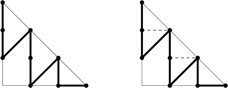
Example 2.
Let us compute for the polygon depicted on Figure 2 in two different ways. Using for a small we get the left two paths depicted on Figure 2. Using we get the three right paths. The corresponding multiplicities are shown under the path. All other -increasing paths have zero multiplicity.

In the next two examples we use as the auxiliary linear function.
Example 3.
Figure 3 shows a computation of the well-known number . This is the number of rational cubic curves through 8 generic points in .

Example 4.
Figure 4 shows a computation of a less well-known number . This is the number of genus 1 quartic curves through 12 generic points in .

4. Real aspects of the count
Suppose that are generic real points. We may ask how many of the relevant complex curves are real, i.e. defined over . Note that this number depends on the configuration of real points.
Theorem 1 can be modified to give the relevant count of real curves. In order to do this we need to define the real multiplicity of a lattice path connecting the vertices and . We introduce the sequence of the pairs of signs (this sequence will record the quadrants of the points ). The sign is prescribed to the edge . We make a convention that and are equivalent if
We set
| (1) |
The definition of the new paths , and the triangle is the same as in section 2. The sign sequence for is , , . The sign sequence for is , . We define the sign and the function as follows.
- •
If all sides of are odd we set and define the sign (up to the equivalence) by the condition that the three equivalence classes of , and do not share a common element.
- •
If all sides of are even we set if . In this case we can ignore (and its sequence of signs). We set if . In this case we define .
- •
Otherwise we set if the equivalence classes of and do not have a common element. We set if they do. In the latter case we define the equivalence class of by the condition that , and have a common element. There is one exception to this rule. If the even side is then there are two choices for satisfying the above condition. In this case we replace in (1) by the sum of the two multiplicities of equipped with the two allowable choices for (note that this agrees with in this case).
Similar to section 2 we define and . As before is a linear map injective on and and are the extrema of .
Theorem 2.
For any choice of and there exists a configuration of of generic points in the respective quadrants such that the number of real curves among the relevant complex curves is equal to the number of -increasing lattice paths connecting and counted with multiplicities .
Example 5.
Here we use the choice so all the points are in the positive quadrant . The first count of from Example 2 gives a configuration of 3 real points with 5 real curves. The second count gives a configuration with 3 real curves as the real multiplicity of the last path is 1. Note also that the second path on Figure 2 changes its real multiplicity if we reverse its direction.
Example 3 gives a configuration of 9 generic points in with all 12 nodal cubics through them real. Example 4 gives a configuration of 12 generic points in with 217 out of the 225 quartics of genus 1 real. The path in the middle of Figure 4 has multiplicity 9 but real multiplicity 1. A similar computation shows that there exists a configuration of 11 generic points in such that 564 out of the 620 irreducible quartic through them are real.
Remark 3.
Real nodal curves have three types of nodes: hyperbolic, elliptic and imaginary. Theorem 2 can be refined to count curves with different types of nodes separately. In accordance with [8] let us prescribe a sign to a real nodal curve, where is the number of its elliptic nodes. To compute the corresponding algebraic number of curves we introduce the multiplicity by replacing (1) with Here we define if at least one side of is even and otherwise. It can be shown with the help of this formula and a combinatorial observation made by Itenberg, Kharlamov and Shustin (to appear) that in the case the algebraic number of irreducible curves counted by is positive for any genus if .
Note that unlike the multiplicity does not depend on the quadrant choices . Furthermore, in [8] Welschinger stated that if then this number is independent of the configuration of generic real points. Corollary 1.2 of [8] combined with Remark 3 implies the following statement (which answers a question asked e.g. by Rokhlin and Kharlamov). For any configuration of generic points in there exists a real rational curve of degree passing through this configuration.
References
- [1] L. Caporaso, J. Harris, Counting plane curves of any genus, Invent. Math. 131 (1998), 345-392.
- [2] I. M. Gelfand, M. M. Kapranov, A. V. Zelevinski, Discriminants, resultants and multidimensional determinants, Birkhäuser Boston 1994.
- [3] M. Kontsevich, Yu. Manin, Gromov-Witten classes, quantum cohomology and enumerative geometry, Comm. Math. Phys. 164 (1994), 525-562.
- [4] M. Kontsevich, Ya. Soibelman, Homological mirror symmetry and torus fibrations, http://arXiv.org math.SG/0011041 Preprint 2000.
- [5] G. Mikhalkin, Gromov-Witten invariants and tropical algebraic geometry (to appear).
- [6] B. Sturmfels, Solving systems of polynomial equations, CBMS Regional Conference Series in Mathematics, AMS Providence, RI 2002.
- [7] R. Vakil, Counting curves on rational surfaces, Manuscripta Math. 102 (2000), 53-84.
- [8] J.-Y. Welschinger, Invariants of real rational symplectic 4-manifolds and lower bounds in real enumerative geometry, (to appear in C. R. Acad. Sci. Paris.) 2003.