Open books and configurationsof symplectic surfaces
Correction to “Open books andconfigurations of symplectic surfaces”
Abstract
We study neighborhoods of configurations of symplectic surfaces in symplectic –manifolds. We show that suitably “positive” configurations have neighborhoods with concave boundaries and we explicitly describe open book decompositions of the boundaries supporting the associated negative contact structures. This is used to prove symplectic nonfillability for certain contact –manifolds and thus nonpositivity for certain mapping classes on surfaces with boundary. Similarly, we show that certain pairs of contact –manifolds cannot appear as the disconnected convex boundary of any connected symplectic –manifold. Our result also has the potential to produce obstructions to embedding specific symplectic configurations in closed symplectic –manifolds and to generate new symplectic surgeries. From a purely topological perspective, the techniques in this paper show how to construct a natural open book decomposition on the boundary of any plumbed –manifold.
Abstract
We correct the main theorem in “Open books and configurations of symplectic surfaces” [1] and its proof. As originally stated, the theorem gave conditions on a configuration of symplectic surfaces in a symplectic -manifold under which we could construct a model neighborhood with concave boundary and describe explicitly the open book supporting the contact structure on the boundary. The statement should have included constraints on the areas of the surfaces.
keywords
Symplectic, contact, concave, open book, plumbing, fillablekeywords
Symplectic, contact, concave, open book, plumbing, fillable57R17 \secondaryclass57N10, 57N13
ATG Volume 3 (2003) 569–586\nlPublished: 20 June 2003
Abstract\stdspace\theabstract
AMS Classification\stdspace\theprimaryclass; \thesecondaryclass
Keywords\stdspace\thekeywords
1 Main Results
All manifolds in this paper are oriented; if is a symplectic –manifold we assume that . By a symplectic configuration in a symplectic –manifold , we mean a union of closed symplectic surfaces embedded in such that all intersections between surfaces are –orthogonal.
A symplectic configuration graph is a labelled graph with no edges from a vertex to itself and with each vertex labelled with a triple , where , and . Associated to a symplectic configuration in a symplectic –manifold is a symplectic configuration graph where each vertex corresponds to a surface , , and , and where each edge represents a point of intersection. Because –orthogonal intersections are necessarily positive, completely determines the topology of a regular neighborhood of (namely, the result of plumbing disk bundles over surfaces according to ); for this much the areas are irrelevant. If we include the area information then also determines the germ of near (due to a slight generalization of standard symplectic neighborhood theorems, as in [10]).
For any vertex in a graph , let denote the degree of , the number of edges connected to . We say that a configuration graph is positive if for every vertex .
Recall that the boundary of a symplectic –manifold is concave (resp. convex) if there exists a symplectic dilation defined on a neighborhood of pointing in (resp. out) along ; this induces a negative (resp. positive) contact structure on .
We present our main theorem in two parts. Part A states that positive symplectic configurations have neighborhoods with concave boundaries, and part B explicitly describes the contact structures on such boundaries in terms of open book decompositions.
Theorem 1.1.
(part A) Given any positive symplectic configuration graph there exists an open symplectic –manifold , a symplectic configuration and a positive contact –manifold , satisfying the following properties:
- •
.
- •
For some contact form for and some (not necessarily smooth) function , letting and , there is a symplectomorphism such that
Thus, given any symplectic configuration in any symplectic –manifold , if then there exists a compact neighborhood of in which is symplectomorphic to a neighborhood of in and which has concave boundary contactomorphic to .
The strength of this theorem will lie in the characterization of in terms of an open book decomposition of . We briefly recall the relationship between contact structures and open books; for more details see [5] and [3].
An open book decomposition of a –manifold is a pair , where is a link and is a fibration such that the fibers are longitudinal near each component of . The link is called the binding and the compact surfaces are called the pages, with for all . By the mapping class group for a compact surface with boundary, we mean the group of orientation-preserving self-diffeomorphisms of fixing pointwise modulo isotopies fixing pointwise. The monodromy of an open book is the mapping class given by the return map of a flow transverse to the pages and meridinal near the binding.
A positive contact form on is supported by the open book if is positive on each page and if orients in the same sense that is oriented as the boundary of a page. A positive contact structure is supported by if for some contact form which is supported by . We have the following result at our disposal:
Theorem 1.2 (Thurston-Winkelnkemper [12], Torisu [13], Giroux [5]).
Every open book decomposition of any –manifold supports some positive contact structure, and any two positive contact structures supported by the same open book are isotopic.
Thus, given a compact surface with boundary and a mapping class , there exists a unique (up to contactomorphism) positive contact –manifold with contact structure supported by an open book with page and monodromy ; we denote this contact manifold .
Given a positive configuration graph , for each vertex let be a surface of genus with boundary components. Let be the surface resulting from performing connect sums between these surfaces, with one connect sum between and for each edge connecting to . Each edge in corresponds to a circle in . An example of a graph and the surface is illustrated in figure 1, with the circles corresponding to the edges drawn in dashed lines.

Let be the product of one right-handed Dehn twist around each of the circles in corresponding to the edges of , let be the product of one right-handed Dehn twist around each component of and let .
Theorem 1.1\qua(part B)\qua
Note that the area information recorded in the graph is not recorded on the boundary . For this reason, we may suppress mention of the areas and think of the vertices of as labelled with pairs , rather than triples .
After proving theorem 1.1 we will briefly discuss the situation when is not positive.
Theorem 1.1 also has purely topological content, namely the explicit characterization of an open book on the boundary of a plumbed –manifold corresponding to a positive configuration graph. If we are only interested in smooth topology, the techniques used to prove theorem 1.1 do yield a theorem characterizing open books on the boundaries of arbitrary plumbed –manifolds, which we now state.
Let a plumbing graph be a graph with no edges connecting a vertex to itself, with each vertex labelled with a pair and with each edge labelled with a or a . The plumbed –manifold corresponding to is a neighborhood of a configuration of surfaces corresponding to the vertices of , with , and each (resp. ) edge corresponding to a positive (resp. negative) transverse intersection between two surfaces. For each vertex let be the signed count of edges connecting to (a edge contributes while a edge contributes ). For each let be a surface of genus with boundary components and let be the result of performing connect sums between these surfaces according to . Let be the product of the following Dehn twists: one right-handed Dehn twist about each circle in corresponding to a edge in , one left-handed Dehn twist about each circle in corresponding to a edge, one left-handed Dehn twist about each boundary component coming from a vertex for which , and one right-handed Dehn twist about each boundary component coming from a vertex for which .
Theorem 1.3.
Given any plumbing graph , let be the associated plumbed –manifold. Then has an open book decomposition with page and monodromy .
In the case where for all vertices, this is in fact giving us a fibration of over , or an “open book with empty binding”. If we apply theorem 1.3 to a positive symplectic configuration graph, the reader may notice that the monodromy as described here is the inverse of the monodromy as described in theorem 1.1; this is because here we are describing whereas in theorem 1.1 we are describing .
The author would like to thank A. Stipsicz for suggesting the idea of trying to understand boundary behaviors for neighborhoods of symplectic configurations as a way to search for new symplectic surgeries, and would like to thank A. Stipsicz, G. Matic, M. Symington and R. Kirby for helpful discussions and for looking at drafts of this paper and suggesting improvements.
2 Applications
Before presenting the main proofs we investigate a few consequences of theorem 1.1 and point out some directions in which to look for further applications.
Given a compact surface , we say that a mapping class is positive if can be expressed as a product of right-handed Dehn twists. It is not hard to show, using compact Stein surfaces and Legendrian surgeries, that if is positive then is strongly symplectically fillable (see [7], [1] and [3]).
Given a configuration graph , let be the associated intersection form; i.e. , where and is the number of edges connecting to . Let denote the number of positive eigenvalues of .
The following is a straightforward application of the adjunction inequality (see [9]):
Corollary 2.1.
Let be a connected positive graph with and with at least one vertex for which . Then is not strongly symplectically fillable and therefore is not positive in .
Proof of corollary 2.1.
The symplectic manifold constructed in theorem 1.1 is open; a function on gives a compact version where . Suppose that is strongly symplectically fillable. Then there exists a closed symplectic –manifold containing for some function on and containing the configuration . The intersection form for is ; since we know that . Thus the adjunction inequality applies, which states that, for any closed surface (with not torsion in if ), . However, here we have an embedded surface for which , which is a contradiction. ∎
Remark 2.2.
For any surface , let us call a relation in of the form a boundary-interior relation if is a single right twist about each boundary component and is some word in interior right twists. We have the following trivial observation: For a given , is positive if and only if there exists a boundary-interior relation in such that the word includes all the twists in . (The order in which the twists of appear in does not matter.) Boundary-interior relations have a variety of uses, including giving constructions of topological Lefschetz pencils (see [3]).
Let denote a surface of genus with boundary components. Two boundary-interior relations are the “lantern relation” in and the “chain relation” in (see [14]).
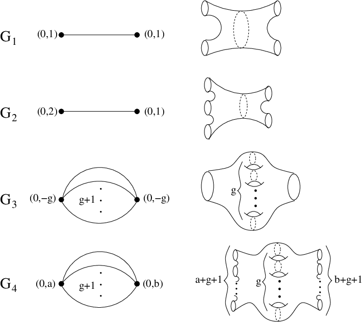
Figure 2 shows a set of example graphs , , , on the left (here we have suppressed the areas and only given the pair at each vertex), with the associated surfaces drawn on the right. The lantern relation shows that is positive, while corollary 2.1 tells us that is not positive. Thus there does not exist a lantern-type relation on . The chain relation shows that is positive (where has edges between vertices so that ). The graph also has edges connecting two vertices, but now the self-intersections are arbitrary integers and such that and . If and are positive and , then and corollary 2.1 tells us that is not positive. Thus, if , , and , then there cannot exist a boundary-interior relation in if contains twists along disjoint curves which, collectively, separate into two genus pieces one containing of components of and the other containing components.
The existence of an elliptic Lefschetz pencil on with points in the base locus and singular fibers means that there exists a boundary-interior relation in such that is the product of twists along curves . This author is not aware that this relation has been written down and has been curious for a long time as to where these curves are. We do know that when we blow up the points we get a Lefschetz fibration given by the relation in , where is a meridinal right twist and is a longitudinal right twist, so that, after embedding in the odd ’s are isotopic to meridians and the even ’s are isotopic to longitudes. Corollary 2.1 gives a little more information, ruling out certain possible arrangements of curves. For example, the observation from the previous paragraph about shows that no two of the curves may be disjoint and separate boundary components from the other . Other possibilities can be ruled out by considering various cycle graphs.
Along much the same lines, we have:
Corollary 2.3.
Let and be positive, connected symplectic configuration graphs with and , with at least one vertex in for which . Then, although each may be strongly symplectically fillable, there does not exist a connected symplectic –manifold with disconnected convex boundary .
Proof.
If such a symplectic –manifold existed then there would exist a closed, connected, symplectic –manifold containing
for appropriate functions and . The intersection form for is , so that ; the rest of the contradiction is identical to that in the preceding proof. ∎
Remark 2.4.
McDuff [8] has shown that symplectic –manifolds with disconnected convex boundary do exist. By a result of Gromov [6] (made explicit in [2] and [8]), it is not possible to have multiple convex boundary components, which is the case of this corollary when and are both disks. We hope that our result significantly enlarges the class of pairs of contact manifolds which cannot appear as disconnected convex boundaries, despite being individually strongly symplectically fillable. It is not hard to construct examples of graphs with , with one vertex for which and such that is not , but it is then not necessarily clear how to show that is in fact strongly symplectically fillable.
It would be interesting to construct arguments in the opposite direction:
Question 2.5.
Are there any positive configuration graphs for which we can show directly that is overtwisted and hence conclude, without appealing to the adjunction inequality, that a symplectic configuration with configuration graph cannot embed in a closed symplectic –manifold?
Showing that is overtwisted for a given surface and mapping class is, in principle, purely a mapping class group problem, as follows: Let and be compact surfaces with boundary and and be mapping classes. We say that is a positive (resp. negative) stabilization of if is the result of attaching a –handle to and , where is a right-handed (resp. left-handed) Dehn twist along a curve dual to the co-core of the –handle. It can be shown, using results of Giroux [5] and Torisu [13], that is overtwisted if and only if there exist pairs and such that is related to by a sequence of positive stabilizations and destabilizations and is a negative stabilization of
Lastly, we point out that theorem 1.1 could be used to produce new symplectic surgeries. If, for a given symplectic configuration graph , we can find some other interesting symplectic –manifold with concave boundary contactomorphic to , then we may surger out a neighborhood of a configuration for which and replace it with . (Symington [10, 11] has investigated configurations which have neighborhoods with convex boundaries, and has used this to produce useful symplectic surgeries; this paper is partly inspired by that work.)
Question 2.6.
Given , is there any canonical way to produce such a with significantly different topology from ? Especially interesting would be examples where is a rational homology ball.
3 The main proof
Proof of theorem 1.1.
Our proof is a three step construction. In “Step 1” we construct a symplectic –manifold with a symplectic dilation (Liouville vector field) defined on all of and pointing out along . will contain a configuration of properly embedded symplectic surfaces with boundary, which will become the configuration once we cap off the surfaces with –handles. In “Step 2”, we arrange that the induced positive contact form on has a particularly nice form and then we produce a symplectic contraction defined on , pointing out along . In “Step 3” we cap off the surfaces in by attaching appropriately framed –dimensional symplectic –handles along ; these handles have the effect of turning the convex boundary into a concave boundary. The symplectic contraction from Step 2 extends across the –handles; flow along gives the symplectomorphism (after attaching an open collar to the boundary).
Step 1\quaFor lack of a better term, the objects we construct in this step will be called “Step 1 objects”. A Step 1 object is a –tuple where:
- •
is a compact symplectic –manifold with boundary.
- •
is a configuration of symplectic surfaces with boundary, each properly embedded in , with –orthogonal intersections.
- •
is a proper Morse function on which restricts to each as a proper Morse function, with only critical points of index and , all of which lie in .
- •
is a symplectic dilation on , tangent to and gradient-like for , inducing a positive contact structure on .
- •
is a fibration such that is an open book on .
- •
is supported by .
Each component of has two different natural framings, the framing coming from the page of the open book, which is a Seifert surface for , and the framing coming from a Seifert surface for . Denote the former framing (for “page framing”) and denote the latter framing (for “component framing”).
Our goal is to produce a Step 1 object related to the given graph as follows:
- •
, where each surface corresponds to a vertex in and the intersections correspond to the edges in .
- •
- •
has components.
- •
For each , there is one component of for which , and for all other components the two framings are equal.
Topologically is built from –handles and –handles, with one –handle for each vertex and each edge in , and with a –handle connecting an edge –handle to a vertex –handle if that edge is incident with that vertex.
We begin with two basic Step 1 objects and defined as follows (here we use polar coordinates on ):
- •
.
- •
.
- •
and .
- •
.
- •
.
- •
while .
Thus is the standard open book on with page equal to a disk and binding the unknot, and is the open book on with page equal to an annulus (a left-twisted Hopf band), monodromy equal to a single right twist about the core circle of the annulus, and the Hopf link with positive linking number as the binding. Note that, for the single component of , we have , whereas for each of the two components of , we have .
We think of these two objects as –dimensional symplectic –handles, in the sense of Weinstein [15]. We also have Weinstein’s –dimensional symplectic –handle, which is constructed as a neighborhood of the origin in with the standard symplectic form , the Morse function and the symplectic dilation . Weinstein shows that we can always attach such a –handle at any two points on a convex boundary of a symplectic –manifold, such that the symplectic forms and symplectic dilations match up along the glueing. In [3] we have shown that, if in addition the contact structure on the boundary is supported by an open book and the attaching –balls of the –handle are pierced by the binding (as the –axis pierces the unit ball in ), then the handle can be constructed in such a way that the new contact structure produced by the associated contact surgery is also supported by an open book. The new page is produced from the old page by attaching a –dimensional –handle at the corresponding intervals along the binding and the new monodromy is equal to the old monodromy extended by the identity on the –handle. (Note that the –dimensional –handle is explicitly the set inside the –dimensional –handle, and that this a symplectic surface.)
Now suppose that we are attaching such a –handle to a Step 1 object at two points along the binding (not connecting two surfaces in that already intersect). Then we produce a new Step 1 object , where is the result of attaching a –handle to , is the open book described in the preceding paragraph, and has a single new index critical point.
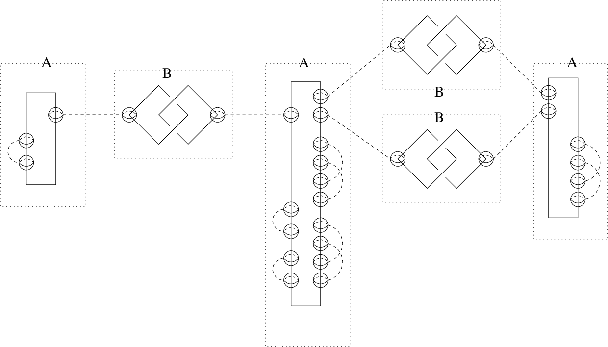
We now describe how to build our desired Step 1 object corresponding to the given graph . Figure 3 illustrates this construction applied to the graph of figure 1. Start with a Step 1 object which is a disjoint union of many copies of the –handle objects and , with one for each vertex and one for each edge in . These are indicated in figure 3 by dotted rectangles, with the bindings of the open books indicated as solid links (unknots or Hopf links). For an edge connecting two vertices and , let be the corresponding copy of and and be the corresponding copies of . Connect to by a symplectic –handle as described above, with the –handle connecting one component of the binding in to the binding in , and connect to by a –handle connecting the other component of the binding in to the binding in . In figure 3 we have drawn the attaching –balls of these –handles with dashed lines connecting them. After doing this for all the edges, we have a Step 1 object where the configuration is a configuration of disks, one disk for each vertex, with intersections given by . Furthermore, for each component of corresponding to a vertex , we have . Now attach –handles in pairs along each component of to get a Step 1 object for which the configuration is now a configuration of surfaces where each corresponds to a vertex , each has a single boundary component, and , with the intersections given by . These pairs of –handles are drawn on the lower right of each binding. We still have . Finally, attach –handles along an isolated stretch of to get binding components for each ; for the “new” binding components we will have , while one binding component still has . These –handles are drawn on the lower left of each binding.
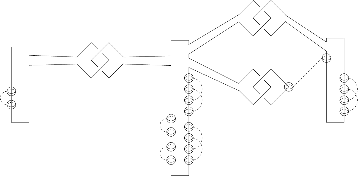
Figure 4 shows a standard Kirby calculus diagram for the same construction, drawn in a single copy of ; the link drawn is the binding of an open book, not a surgery link (yet).
Note that the page of the resulting open book in the final Step 1 object is exactly the surface associated to the graph and that the monodromy is exactly the mapping class . Thus .
Step 2\quaFor each in , choose a positive constant . By an explicit construction (similar to that in section 4 of [3]) one can show that there exists a positive contact form supported by with the following behavior near each component of each : In a neighborhood of there should exist solid torus coordinates (radial, meridinal and longitudinal coordinates, with with respect to which and . After an isotopy fixing , by theorem 1.2, we can assume that . Because is defined on all of and is gradient-like for , we can use the canonical symplectification of and enlarge and/or trim so that in fact .
At this point note that the area of each is .
Now we recall some definitions from [4]. A contact pair on a –manifold is a pair of –forms defined, respectively, on open subsets with , such that on and such that on . In particular (resp. ) is a positive (resp. negative) contact form and is a closed, nowhere zero –form on . A dilation-contraction pair on a symplectic –manifold is a pair defined, respectively, on open subsets , such that and . We say that transversely covers a –dimensional submanifold if and both and are positively transverse to . This gives us an induced contact pair on defined by , with domains .
In our situation we have the positive contact form defined on , supported by ; for a large enough constant , will be a contact pair (with ). Fix such a and henceforth let .
Backward flow along the symplectic dilation starting on gives us an embedding such that , and , where is the coordinate on . Since is tangent to and gradient-like for , we know that . Lemma 4.1 in [4] then tells us that there exists a unique symplectic contraction defined on such that is a dilation-contraction pair transversely covering inducing the contact pair . Forward flow along starting on then gives an embedding from into for some function , such that , and . The proof of lemma 4.1 in [4] shows us how to explicitly calculate given , from which we can see that, in our case, and the image of is all of , with .
Step 3\quaOur final symplectic –manifold will be constructed by attaching a symplectic –handle as described in [4] along each component of the binding with framing , and then attaching an open symplectic collar on the boundary. In [4] it is shown that one can attach handles in this way to produce a concave boundary, and in [3], it is shown that the contact manifold on the boundary is indeed . It is not hard to see that the –manifold produced in this way is a neighborhood of a configuration of closed surfaces with the correct genera and intersecting according to the graph ; the surfaces are simply the surfaces in capped off with the descending disks of the –dimensional –handles.
To see that the self-intersections are correct, note that the self-intersection of a surface built by attaching –handles, framed as above, along for one of the surfaces is equal to the sum over all components of of , which is exactly .
To see that the remaining claims of the theorem hold, we need to look more closely at the structure of the –handles. Proposition 4.6 in [4] shows us how to construct our –handles; here we give the construction tailored to the special case at hand. For each , let (with as fixed in Step 2). The handle that will attach to each component of is a subset of with the symplectic form with the Morse function . The following is a dilation-contraction pair on :
transversely covers the regular level sets of as long as . Let ; note that . Choose some with . Construct so that the attaching boundary of (which we call ) is a neighborhood of in and so that the free boundary interpolates from a neighborhood of in down to , so that both boundaries are transverse to both and (where defined). (See section 2 of [4] for a more detailed discussion of this type of handle construction and notation.) On , we use solid torus coordinates ; the contact pair induced by on then becomes:
This is exactly the contact pair we have on a neighborhood of , so that lemma 4.1 in [4] tells us we can attach to by identifying the coordinates on with the coordinates in a neighborhood of , in such a way that the symplectic forms and the dilation-contraction pairs fit together smoothly. Note that since in a neighborhood of , we are attaching with framing .
After attaching these handles to each component of , we get a closed surface which is the union of and the disks in each handle . is smooth because is tangent to and is tangent to . is symplectic because and are both symplectic. We have already arranged that the area of is . The area of each disk is . Thus the area of is exactly . Let .
Note that, in the handle , the symplectic contraction is defined across all of the free boundary whereas the dilation does not extend across the ascending circle . Thus after attaching all the handles we get a symplectic –manifold with a dilation-contraction pair which transversely covers inducing a contact pair with domains (where is the union of the ascending circles) and . The closed –form is for the natural open book on that results from surgeries on the binding of the open book on , the pages of which are still diffeomorphic to and the monodromy of which is now (see [3]). The fact that is a contact pair implies that , which in turn implies that , as a positive contact form on , is supported by the open book , which has page and monodromy . Thus we let and . Also let .
From the explicit form for and the observations made in Step 2 about flow along , we see that flow along starting on gives a diffeomorphism from to , for some function , such that , , and .
Finally let ; the embedding is simply extended by the identity on .
∎
4 The nonpositive case
If our initial graph is not positive, we can simply add extra vertices labelled to produce a graph which is positive. This corresponds to plumbing on some extra spheres of square . We can now carry out the construction above applied to , but stop short of attaching the –handles required to close off these extra spheres. This will give a model neighborhood of a configuration with , but now the boundary will not be concave. Instead the boundary will be “partially convex and partially concave” in the following sense: will carry a dilation-contraction pair transversely convering inducing a contact pair , but neither nor will be defined on all of . Nevertheless, the pair will determine the germ of along and the dilation-contraction pair determines something like a canonical symplectification of the contact pair, so that we have good control on the symplectic topology of . Furthermore, will be supported by a signed open book on , by which we mean the following: is an open book, is defined on , and is supported, as a positive contact form on , by . The link will be the union of the ascending circles for the –handles that we did attach, while will be the binding components from the Step 1 object to which we did not attach –handles. Smaller or larger neighborhoods of will have boundaries which are still transversely covered by the dilation-contraction pair and hence carry related contact pairs, all supported by the same signed open book. This line of reasoning will be investigated more thoroughly in a future paper.
5 Boundaries of arbitrary plumbings
Proof of theorem 1.3.
If we strip the symplectic topology out from the proof of theorem 1.1, Step 2 is irrelevant. In Step 1, relabel as and introduce a negative version of which we call ; (resp. ) is a neighborhood of a positive (resp. negative) intersection of two disks, with a left-twisted (resp. right-twisted) Hopf band as the open book on the boundary, with monodromy equal to a single right (resp. left) Dehn twist along the core of the band. On we have and on we have . Thus if we mimic the construction in theorem 1.1 but use copies of for edges and copies of for edges, we can produce a (non-symplectic) Step 1 object where:
- •
is a compact –manifold with boundary which is a neighborhood of .
- •
is a configuration of properly embedded surfaces with boundary, corresponding to the vertices of , with the appropriate genera and self-intersections and intersecting transversely according to the edges of .
- •
has components, unless , in which case has one component. (Recall that now is the signed count of edges connecting to .)
- •
is a fibration making an open book on .
- •
For each , there is one component of for which and for all other components the two framings are equal.
When we get to Step 3, since we are no longer requiring that our handles be symplectic, we can attach –handles along binding components with any framings we choose. Framing produces a new open book with the same page and introduces a right-handed boundary Dehn twist into the monodromy; framing also produces a new open book with the same page and introduces a left-handed boundary Dehn twist. Framing produces a new open book with the page alterred by capping off the corresponding boundary component, decreasing the number of binding components by . For vertices with , use -framed binding handles, for vertices with , use -framed binding handles and for vertices with , use -framed binding handles. Because of these choices of framings we then calculate that for each , . ∎
References
- [1] Selman Akbulut, Burak Ozbagci, On the topology of compact Stein surfaces, Int. Math. Res. Not. (2002) 769–782
- [2] Yakov Eliashberg, Filling by holomorphic discs and its applications, from: “Geometry of low-dimensional manifolds, 2 (Durham, 1989)”, Cambridge Univ. Press, Cambridge (1990) 45–67
- [3] David T Gay, Explicit concave fillings of contact three-manifolds, Math. Proc. Cambridge Philos. Soc. 133 (2002) 431–441
- [4] David T Gay, Symplectic 2-handles and transverse links, Trans. Amer. Math. Soc. 354 (2002) 1027–1047 (electronic)
- [5] Emmanuel Giroux, in preparation
- [6] M Gromov, Pseudoholomorphic curves in symplectic manifolds, Invent. Math. 82 (1985) 307–347
- [7] Andrea Loi, Riccardo Piergallini, Compact Stein surfaces with boundary as branched covers of , Invent. Math. 143 (2001) 325–348
- [8] Dusa McDuff, Symplectic manifolds with contact type boundaries, Invent. Math. 103 (1991) 651–671
- [9] Dusa McDuff, Dietmar Salamon, Introduction to symplectic topology, second edition, Oxford University Press, Oxford (1998)
- [10] Margaret Symington, Symplectic rational blowdowns, J. Differential Geom. 50 (1998) 505–518
- [11] Margaret Symington, Generalized symplectic rational blowdowns, Algebr. Geom. Topol. 1 (2001) 503–518 (electronic)
- [12] W P Thurston, H E Winkelnkemper, On the existence of contact forms, Proc. Amer. Math. Soc. 52 (1975) 345–347
- [13] Ichiro Torisu, Convex contact structures and fibered links in 3-manifolds, Internat. Math. Res. Notices 2000 (2000) 441–454
- [14] Bronislaw Wajnryb, An elementary approach to the mapping class group of a surface, Geom. Topol. 3 (1999) 405–466 (electronic)
- [15] Alan Weinstein, Contact surgery and symplectic handlebodies, Hokkaido Math. J. 20 (1991) 241–251
Received:\qua27 January 2003
57R17 \secondaryclass57N10, 57N13 \agt ATG Volume 3 (2003) 1275–1276\nlPublished: 20 December 2003
Abstract\stdspace\theabstract
AMS Classification\stdspace\theprimaryclass; \thesecondaryclass
Keywords\stdspace\thekeywords
In the paper being corrected [1], we considered symplectic configuration graphs where each vertex was decorated with a triple , being the genus of a surface, its self-intersection, and its symplectic area. Theorem 1.1 in [1] is false as stated. However we have the following:
Correction 1.
The conclusions of theorem 1.1 (parts A and B) are true if we add the hypothesis that there exists a constant such that, for each , .
An easy counterexample to the theorem as originally stated is given by two surfaces and , with and . If , then when restricted to the boundary of a neighborhood of , because is nonzero when evaluated on the class , which lives on the boundary. In general, this problem occurs when the intersection matrix for the configuration of surfaces has determinant equal to zero.
The error is on line 4 of page 583 in [1], in the calculation of . The correct statement is:
Thus, to arrange that this agree with the contact pair we already have on a neighborhood of , we are forced to choose , as opposed to , which was the choice made on page 582 line 22. With , we get that the area of is . After the construction we can rescale by a constant to get the area to be .
Note that, if the configuration is contained in a closed symplectic -manifold , then the area condition added in this correction is equivalent to the condition that is Poincaré dual to some multiple of , where is a class with for . This is because .
Here we emphasize that this correction does not affect the applications in section 2 of [1], or forthcoming applications in [2].
References
- [1] D T Gay Open books and configurations of symplectic surfaces, Alg. Geom. Top. 3 (2003), 569–586
- [2] D T Gay and R Kirby Constructing symplectic forms on 4-manifolds which vanish on circles, to appear
Received:\qua1 December 2003