Heegaard Floer homology and alternating knots
Abstract
In an earlier paper, we introduced a knot invariant for a null-homologous knot in an oriented three-manifold , which is closely related to the Heegaard Floer homology of . In this paper we investigate some properties of these knot homology groups for knots in the three-sphere. We give a combinatorial description for the generators of the chain complex and their gradings. With the help of this description, we determine the knot homology for alternating knots, showing that in this special case, it depends only on the signature and the Alexander polynomial of the knot (generalizing a result of Rasmussen for two-bridge knots). Applications include new restrictions on the Alexander polynomial of alternating knots.
keywords
Alternating knots, Kauffman states, Floer homologyDepartment of Mathematics, Princeton University
New Jersey 08540, USA \secondemailszabo@math.princeton.edu
57R58\secondaryclass57M27, 53D40, 57M25
eometry & opology Volume 7 (2003) 225–254\nlPublished: 24 March 2003
Email:\stdspace\theemail
URL:\stdspace\theurl
Abstract
AMS Classification numbers Primary: \theprimaryclass
Secondary: \thesecondaryclass
Keywords \thekeywords
Proposed: John Morgan Received: 1 November 2002\nlSeconded: Yasha Eliashberg, Robion Kirby Revised: 19 March 2003
1 Introduction
In [25], we introduced a collection of Abelian groups associated to a closed, oriented three-manifold , the Heegaard Floer homology of .11 1 In most of this paper, we work with the simplest version of Heegaard Floer homology, , for three-manifolds with . In this case is a -graded, finitely generated Abelian group. In [27], we introduced a “knot filtration” on the Heegaard Floer homology of a three-manifold which is induced from a null-homologous knot in , see also [30]. Taking the homology groups of the associated graded object, we obtain Floer homology groups (where the integer appearing here corresponds to the filtration level) which are topological invariants of the knot .
Our aim here is to study these invariants in the case where the ambient three-manifold is the three-sphere, in which case . Working with a suitable Heegaard diagram compatible with a planar projection of the knot, we describe the “classical” aspects of the Floer theory – generators of the knot complex, their filtration levels, and absolute gradings – in terms of combinatorics of a (generic) knot projection to the plane (though the differentials in the knot complex still elude such a description). With this combinatorial description in hand, we are able to completely determine the Heegaard Floer homology for alternating knots – i.e. those which admit a projection for which the crossing types alternate between overcrossings and undercrossings – and give some topological applications. More calculations based on these descriptions will be given in a future paper [29].
1.1 Classical Floer data for classical knots
Let be a knot. To define the knot Floer homology, we must work with a Heegaard diagram for which is compatible with the knot . Specifically, we require that the knot is supported entirely inside one of the two handlebodies, meeting exactly one of the attaching disks in a single transverse intersection point. As in [27], we then obtain a set of generators of the chain complex (the chain complex whose homology calculates ), which are endowed with a pair of integer-valued functions, the filtration level and the absolute grading .
For the boundary operator on , if corresponds to a generator and appears with non-zero multiplicity in the expansion of , then , while . Thus, the associated graded complex for the filtration , which we denote here by , is also freely generated by , but its boundary operator now preserves , and hence we have the splitting
where is the subcomplex generated by elements with . We reiterate: although this associated chain complex depends on the choice of Heegaard diagram used for , its homology
does not.
A decorated projection for is a generic knot projection of , together with a choice of a distinguished edge. In Section 2, we associate a natural Heegaard diagram for to any decorated knot projection for . This allows us to describe the generators and the functions and in terms of the knot projection. For the description of the generators, we use the notion of states introduced by Kauffman for the Alexander polynomial, see [16]. We recall this briefly here.
Let be an oriented knot, and fix a decorated projection of . The projection gives a planar graph whose vertices correspond to the double-points of the projection of . Since is four-valent, there are four distinct quadrants (bounded by edges) emanating from each vertex, each of which is a corner of the closure of some region of . Let denote the number of vertices of . Clearly, divides into regions. The two regions which share the distinguished edge will be denoted and . In fact, we will always choose our projections so that is the unbounded region.
Definition 1.1.
A Kauffman state (cf. [16]) for a decorated knot projection of is a map which associates to each vertex of one of the four in-coming quadrants, so that:
- •
the quadrants associated to distinct vertices are subsets of distinct regions in
- •
none of the quadrants is a corner of the distinguished regions or .
It is easy to see that a Kauffman state sets up a one-to-one correspondence between vertices of and the connected components of . There is a very simple description of Kauffman states in graph-theoretic terms (see also [16]). The regions in the complement of the planar projection can be colored black and white in a chessboard pattern, by the rule that any two regions which share an edge have opposite color. There is then an associated “black graph”, whose vertices correspond to the regions colored black, and whose edges correspond to vertices in which connect the opposite black regions. In these terms, Kauffman states are in one-to-one correspondence with the maximal subtrees of the black graph (under a correspondence which associates to a Kauffman state the union of vertices of , thought of now as edges in the black graph, to which associates a black quadrant).
Let denote the set of Kauffman states for our decorated knot projection. We define two functions and , called the filtration level and absolute grading respectively.
To describe the filtration level, note that the orientation on the knot associates to each vertex a distinguished quadrant whose boundary contains both edges which point towards the vertex . We call this the quadrant which is “pointed towards” at . There is also a diagonally opposite region which is “pointed away from” (i.e. its boundary contains the two edges pointing away from ). We define the local filtration contribution of at , denoted by , by the following rule (illustrated in Figure 2), where denotes the sign of the crossing (which we recall in Figure 1):
The filtration level associated to a Kauffman state, then, is given by the sum
Note that the function is the -power appearing for the contribution of to the symmetrized Alexander polynomial, see [1], [17].

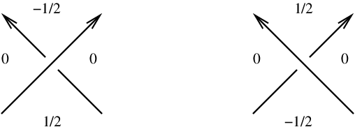
The grading is defined analogously. First, at each vertex , we define the local grading contribution . This local contributions is non-zero on only one of the four quadrants – the one which is pointed away from at . At this quadrant, the grading contribution is minus the sign of the crossing, as illustrated in Figure 3. Now, the grading of a Kauffman state is defined by the formula

With these objects in place, we can now state the following:
Theorem 1.2.
Let be a knot in the three-sphere, and choose a decorated knot projection of . Then, there is a Heegaard diagram for with the property that the knot complex is freely generated by Kauffman states of the decorated projection. Moreover, if denotes the generator of and is its corresponding Kauffman state, then and .
1.2 Heegaard Floer homology for alternating knots
In the special case where the knot is alternating, Theorem 1.2 easily determines the knot homology completely in terms of the Alexander polynomial of the knot and its signature .
In the following theorem, we use the sign conventions according to which the signature of the left-handed trefoil is , cf. [20].
Theorem 1.3.
Let be an alternating knot in the three-sphere, and write its symmetrized Alexander polynomial as
Then, is supported entirely in dimension , and indeed
It is very suggestive to compare the above result with the corresponding theorem of Lee on the Khovanov homology for alternating knots (see [19], see also [18], [2], [13]). We can also use the above theorem to calculate the Heegaard Floer homologies of three-manifolds obtained by zero-surgeries along the knot. In particular, we obtain the following result, which is a generalization of a theorem of Rasmussen (see [30]) which calculates the Heegaard Floer homology of three-manifolds obtained as integer surgeries along two-bridge knots. (In effect, our methods show that alternating knots are “perfect” in Rasmussen’s sense.)
To state our results in a useful form, we recall more aspects of the Heegaard Floer homology package from [25]. Specifically, there is a variant of the Heegaard Floer homology which is a module over the ring . This module is related to the variant considered earlier by a canonical long exact sequence
The group can be given an absolute grading. In fact, these groups obtain some additional structure, depending on the the homological properties of , which we describe now in the case where (as is the case for zero-framed surgery on a knot in ). In this case, there is a splitting with the property that . Indeed, the summand is endowed with a relative grading22 2 Let be an Abelian group. An (absolutely) -graded Abelian group is an Abelian group generated by a set , equipped with a map . A relatively -graded Abelian group is an Abelian group generated by a set , equipped with a relative grading with . (compatible with the mentioned earlier), and in particular when , it gives a relative -grading. Indeed the summand with can be given an absolute grading with values in the set . Although this choice might seem unnatural at first glance, it fits neatly with the four-dimensional theory, cf. [28]. Action by the ring element decreases all of these gradings by .
Let denote the -graded -module which is abstractly isomorphic to , graded so that multiplication by decreasing grading by two, and its bottom-most homogeneous generator has degree . Recall that .
Given a knot and an integer , let denote the torsion coefficients defined by
(where here the are the coefficients of the symmetrized Alexander polynomial of ). These integers are closely related to the Milnor torsion of the knot [21], see also [32].
Finally, for , we let be the integer defined by
| (1) |
Note that is the torsion coefficient of the torus knot.
Theorem 1.4.
Let be an alternating knot, oriented so that , and let denote the three-manifold obtained by zero-surgery on . Then,
- •
for all , we have a -module isomorphism
where the first summand is supported in degree , while the second summand has odd parity, and is defined as in Equation (1),
- •
for , we have an isomorphism of graded modules
and the cyclic summand lies in degree .
Thus, in both cases, is given by the formula
| (2) |
1.3 Applications to the topology of alternating knots
We now describe some of the consequences of the above calculations for alternating knots, combined with other results on Heegaard Floer homology.
As a first consequence, we obtain the following calculation of the “correction terms” for three-manifolds obtained as surgery on along , for any alternating knot . This correction term is defined using the absolute grading on the module when is an integer homology three-sphere, described in [28]. (As explained in that reference, when , the group can be endowed with an absolute -grading.) This number is the analogue of the gauge-theoretic invariant of Frøyshov introduced in [10], [12], constraining the intersection forms of four-manifolds which bound . Specifically, according to Theorem of [28], if is an integer homology three-sphere, then for each negative-definite four-manifold which bounds , we have the inequality
| (3) |
for each characteristic vector for the intersection form .33 3 Recall that for a bilinear form over a lattice , a characteristic vector is a vector with the property that for all . Recall that Elkies [8] proves that for any negative-definite, unimodular form over ,
with equality holding if and only if the bilinear form is diagonalizable (over ). In view of these results, then, bounds the “exoticness” of intersection forms of smooth, definite four-manifolds which bound , providing a relative version of Donaldson’s diagonalization theorem [6], see also [10] and [12].
In general, calculating is challenging. But for surgeries on alternating knots, we have the following explicit result (compare [30], [11]):
Corollary 1.5.
Let be an alternating knot, then
In another direction, Theorem 1.4 can be used to give restrictions on the Alexander polynomials of alternating knots. A classical result of Crowell and Murasugi (see [4] and [22]) states that the coefficients of the symmetrized Alexander polynomial for such a knot alternate in sign (indeed, the sign of is ). Theorem 1.4 in turn immediately gives the following inequality for the torsion coefficients, which is easily seen to generalize this alternating phenomenon:
Corollary 1.6.
Let be an alternating knot in the three-sphere. Then for all , we have that
where are the constants defined in Equation (1).
For example, consider the nine-crossing knot appearing in the standard knot tables as , see for example [3]. This knot has
| and |
i.e. its Alexander polynomial is alternating, but it fails to satisfy the conditions of Corollary 1.6, so it is not alternating. (Note this particular result is classical, see [5].)
Other restrictions on the Alexander polynomials of alternating knots have been conjectured by Fox, see [9] (see also [23], where these properties are verified for a large class of alternating knots). Specifically, Fox conjectures that for an alternating knot, the absolute values of the coefficients of the Alexander polynomial are non-increasing in , for . It is easy to see that the above corollary verifies Fox’s conjecture for alternating knots of genus . For a general alternating knot, the inequalities stated above for coefficients are independent of Fox’s prediction. However, for the first coefficient change, i.e. when , the above inequalities translate into the following stronger bound:
Finally, we describe a relationship between Theorem 1.4 and contact geometry. Recall that a fibered knot endows with an open book decomposition, and hence a contact structure, using a construction of Thurston and Winkelnkemper, see [31]. One can ask which contact structure this is.
For this purpose, recall that a contact structure in has a classical invariant, the “Hopf invariant” of the induced two-plane field , which is an integer which uniquely specifies the homotopy class of . This number is defined by
where is any almost-complex four-manifold which bounds so that the induced complex tangencies on its boundary coincide with , is the canonical class of the almost-complex structure, is the Euler characteristic of , and is the signature of its intersection form.
Using results on the knot homology of fibered knots described in [26] (which, in turn, are based on the important work of Giroux [14]), we obtain the following:
Corollary 1.7.
Let be an alternating, fibered knot of genus , and let denote its induced contact structure over . Then,
| (4) |
Moreover, the induced contact structure on is tight if and only if .
In [7], Eliashberg classifies contact structures over , showing that for each non-zero integer , there is a unique contact structure whose Hopf invariant is , while there are two contact structures with vanishing Hopf invariant: the “standard” (tight) contact structure, and another (overtwisted) one. Combining Corollary 1.7 with Eliashberg’s classification, we obtain the following:
Corollary 1.8.
The standard contact structure and all other contact structures in with negative Hopf invariant are precisely those contact structures which are represented by alternating, fibered knots.
1.4 Alternating links
Theorem 1.3, together with many of its consequences, admits a straightforward generalization to the case of non-split, alternating links. We state and prove the generalization in Section 4. As an illustration, we use this as a stepping-stone for a calculation of the knot homology for a non-alternating knot, .
Acknowledgements\quaThe authors wish to warmly thank Jacob Rasmussen and András Stipsicz for interesting conversations.
PSO was supported by NSF grant number DMS 9971950 and a Sloan Research Fellowship; ZSz was supported by NSF grant number DMS 0107792 and a Packard Fellowship.
2 Proof of Theorem 1.2.
We prove here the state-theoretic interpretation of the classical Floer data, stated in Theorem 1.2. The main ingredient is a Heegaard diagram which is naturally associated to a decorated knot projection. (Note that this is not the usual diagram induced from placing the knot into “bridge position”.) We describe this Heegaard diagram, after briefly recalling some of the ingredients of the knot Floer complex for knots (specializing for simplicity to the case where the ambient manifold is ).
2.1 Classical Floer data.
We give here a rapid description of the data for the knot Floer complex captured in Theorem 1.2. We refer the reader to [27] for a more detailed discussion.
Fix an oriented knot . A marked Heegaard diagram is triple of data
where here
- •
is an oriented surface of genus ,
- •
are pairwise disjoint, embedded circles in representing the attaching circles for a handlebody ; similarly, are pairwise disjoint, embedded circles in representing the attaching circles for a handlebody
- •
is a marked point on the attaching circle , which is disjoint from the
- •
the Heegaard diagram describes , i.e. we have a diffeomorphism
- •
under this identification, the knot is supported entirely inside , and it is disjoint from the attaching disks for with , meeting the attaching disk for in a single positive, transverse intersection point.
We consider the -fold symmetric product , with two distinguished tori
| and |
The generators for the chain complex are intersection points between and in . Let and be two points in which are near , but which lie on either side of . A choice of orientation on gives an ordering on these two points. More precisely, we can find arc connecting to so that is disjoint from all and with , meeting in a single, transverse intersection point. Orienting in the same direction as , we order the two base points so that goes from to .
By simple topological considerations (cf. Section of [25]), given two intersection points , we can find a Whitney disk for and which connects to ; i.e. a map from the standard complex disk into with the properties that
Let be a point in , we let denote the algebraic intersection number of with the submanifold . In fact, by choosing reference points in each connected component of , we obtain a function from this set of regions to , denoted , and called the domain associated to . As explained in Section of [25], when , the homotopy class of is uniquely determined by . We denote the set of homotopy classes of Whitney disks by .
We now describe the functions and , referred to in the introduction. The definitions we sketch here are somewhat simpler than the general definitions given in [27]44 4 In fact, in [27], the filtration is denoted , and in the case we are considering now, it takes values in the set of structures on . This is related to the present function by the formula where here is the closed surface in obtained by capping off a Seifert surface for which respects the orientation of ., owing to the fact that our ambient manifold is .
First, we discuss . Given and , let be a Whitney disk connecting to . We claim that if denotes the Maslov index of , then is independent of the choice of . Indeed (cf. Equation () of [25]), the function is determined up to an additive constant by the relation
The remaining indeterminacy is removed using the Heegaard Floer homology of : is a chain complex which is generated by the same intersection points (though its boundary operator allows for more differentials than the knot Floer complex ), its boundary operator decreases by one, and its homology is , supported in a single dimension. The indeterminacy, then, is removed by the convention that the homology is supported in dimension zero.
Similarly, if and are a pair of intersection points and is a Whitney disk connecting them, then we claim that the difference of intersection numbers is independent of the choice of . Indeed (cf. Lemma of [27]), the function is determined up to an additive constant, by the equation
The remaining indeterminacy of is removed with the help of the observation that
where here denotes the symmetrized Alexander polynomial of (see Equation () of [27]), and is some integer. The additive indeterminacy of , then, is removed by requiring that .
We have not defined here the differential on the chain complex. Loosely speaking, the differential on counts pseudo-holomorphic Whitney disks with , while the differential on counts those which satisfy . Details are given in [27].
2.2 The Heegaard diagram belonging to a decorated knot projection
Let be an oriented knot in , and fix a decorated knot projection of – i.e. a generic planar projection of with crossings, and a choice of distinguished edge which appears in the closure of the unbounded region . With these choices, we construct a Heegaard diagram for as follows.
Let denote the other region which contains the edge , and let be the boundary of a regular neighborhood in of (i.e. it is a surface of genus ); we orient as . We associate to each region , an attaching circle (which follows along the boundary of ). To each crossing in we associate an attaching circle as indicated in Figure 4. In addition, we let denote the meridian of the knot, chosen to be supported in a neighborhood of the distinguished edge .
Each vertex is contained in four (not necessarily distinct) regions. Indeed, it is clear from Figure 4, that in a neighborhood of each vertex , there are at most four intersection points of with circles corresponding to these four quadrants. (There are fewer than four intersection points with if is a corner of the unbounded region .) Moreover, the circle corresponding to meets the circle in a single point (and is disjoint from the other circles). It is easy to see that for any choice of marked point , the construction we have just described gives a marked Heegaard diagram for .
The correspondence between states and generators for the knot complex, , should now be clear: an intersection point gives at each vertex (i.e. -curve) one of four quadrants (corresponding to the up to four -curves). Moreover, since the meridian meets exactly one -curve, the curve corresponding to the region , that corresponding -curve is not assigned to any of the vertices.
 \relabel
r1 \relabelr2 \relabelr3 \relabelr4 \adjustrelabel¡-2pt,0pt¿ a1 \adjustrelabel¡-2pt,0pt¿ a2 \relabela3 \relabela4 \relabelb \endrelabelbox
Before turning to the other aspects of Theorem 1.2, we recall a very useful technical device: the “Clock Theorem” of Kauffman.
Definition 2.1.
Two distinct states and are said to differ by a transposition if there is a pair of vertices to with the property that:
- •
,
- •
there is a straight path from to (i.e. a path which follows along the knot ) which does not contain the distinguished edge, so that and are the two quadrants which contain the first edge in , and and are the two quadrants which contain the last edge in .
Theorem 2.2 (Kauffman).
Any two distinct states and can be connected by a sequence of transpositions.
The proof of the above result can be found in Chapter 2 of [16].
We now establish some lemmas used in the proof of Theorem 1.2.
Lemma 2.3.
Suppose that the two states and differ by a transposition, and let and denote the corresponding generators of the knot complex. Then, .
Proof.
Orient the edge between and as it appears in the knot. There are now four cases, according to whether or are under- or over-crossings.
Suppose that the edge takes us from under-crossing at to an over-crossing at (i.e. our edge is on the bottom at and on the top at ). In this case, we claim that after possibly switching the roles of and , we can find a homotopy class , with and . Indeed, the domain associated to , , has all local multiplicities zero or one; topologically, it is a connected surface with a collection of circle boundary components. Assume for a moment that there are no intermediate crossings between and . In this case, the topology of is given as follows: the genus of is given by the number of vertices encountered twice between and the final point, it has one boundary component corresponding to the meridian , it has one boundary circle for each vertex encountered only once between and the final point (the corresponding -circle), and there is one final boundary component (with four distinguished corner points) which is formed from arcs in , , and the two -curves corresponding to the two regions which contain the edge from to . This is pictured in Figure 5. In the case where there are intermediate crossings between and , the surface looks much the same, except that now there are additional circle components, one corresponding to each compact region in the complement in of the part of the projection between and (or equivalently, one for each vertex between and ). Specifically, these circle components are the -curves of these intermediate regions.
The detailed description of the topology of is not particularly relevant to the proof of the present lemma (though it is relevant in the proof of the next one); all we need here is the fact that and , from which it follows immediately that . From the definition of , it follows easily that (i.e. independent of the orientation on the two pieces of transverse to our edge at and ) as well, verifying the lemma in this case.
Suppose that both and are under-crossings. When there are no intermediate intersection points between and , it is easy to find a square which serves as for some with , supported on the region of the Heegaard surface corresponding to the edge, as pictured in Figure 5. In particular, the filtration difference is zero. When there are intermediate intersection points, the region now is a square with a finite number of circles removed, but it is still disjoint from and . Now, it is easy to see that the formula gives zero, independent of the crossing signs of the two vertices.
The remaining two cases (where is an over-crossing) are handled similarly. ∎

Lemma 2.4.
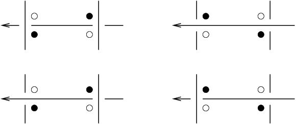
Suppose that the two states and differ by a transposition, at vertices and . Then, the absolute value of the difference in gradings between the corresponding generators in is one. More precisely, if is represented by light dots in Figure 6, and is represented by the dark ones, then .
Proof.
Domains with connecting intersection points which differ by a transposition have already been demonstrated in the proof of Lemma 2.3 (see Figure 5). Our task here is to calculate their Maslov index (and, indeed, to show that it is one in all the above cases).
In all cases, we have seen that the domains are topologically a square with a finite number of handles attached, and a finite number of disks removed. Letting denote the intersection points corresponding to the states and , and writing , and , we have (for some numbering) that for , , while , , , and are the four corner points of the square. Now, in the interior of each handle attached to the square, we have a point (for ), and also on each circle we have a point , and all the remaining intersection points (with ) lie in the exterior of . Thus, these extra intersection points do not affect the Maslov index. Moreover, each of the handles can be deleted, while deleting the corresponding intersection point without affecting the Maslov index. (This latter operation corresponds to destabilizing the Heegaard diagram, see [25].)
It remains then to calculate the Maslov index of a homotopy class whose domain consists of square minus a finite collection of disks. We claim that for such a homotopy class, . This can be seen, for example, by finding such a homotopy class in a suitably chosen (genus ) Heegaard diagram for (where here denotes the number of disks removed), and using the fact that as relatively -graded groups where here denotes the structure with first Chern class equal to zero (cf. Section of [25]). Specifically, we can find such a domain which connects two intersection points whose absolute gradings are known to differ by one. We illustrate this in the case where , in Figure 7. ∎
 \adjustrelabel
¡-2pt, 0pt¿ A1 \adjustrelabel¡-2pt, 0pt¿ A \adjustrelabel¡-2pt, 0pt¿ B \adjustrelabel¡-2pt, 0pt¿ C1 \adjustrelabel¡-2pt, 0pt¿ C \adjustrelabel¡-2pt, 0pt¿ x1 \relabelx2 \relabelx3 \relabely1 \relabely2 \relabelz \endrelabelbox
We find it useful to introduce one more notion before proceeding to the proof of Theorem 1.2. Recall that the decoration on the knot projection (the distinguished edge, and the orientation on the knot projection) induces a natural ordering on all the edges of the knot projection. If is any vertex in the knot projection, the edge after is the last edge (in this ordering) whose closure contains . The edge which immediately precedes it will be called the -penultimate edge, and we denote it by . Note also that the orientation of and the reference point specifies an ordering on the vertices, as follows. We say that if the vertex is crossed the second time before is (on a path beginning in the interior of the distinguished edge and following ).
There is a canonical state which is uniquely characterized by the property that for each crossing , is one of the two quadrants whose closure contains -penultimate edge, according to the following lemma:

Lemma 2.5.
The canonical state is well-defined.
Proof.
Let denote the set of regions in . Let . We will inductively define the canonical state by finding an ordering of all the vertices in the graph , with the property that is uniquely defined (note that it is not the same as the ordering induced by the orientation of ). Correspondingly, we will exhaust by a sequence of regions
with the property that maps onto the set of regions in (and hence is defined by attaching to a region ). In our induction hypothesis, we will assume that the -penultimate edge is contained in the interior of .
For the initial step (), is vacuously defined.
For the inductive step, either (in which case we are finished), or is a proper subset of , in which case it must have corners, since we have assumed that our graph belongs to a knot projection. Consider the last corner point of (with respect to the ordering induced by the orientation on the knot). It is clear that the -penultimate edge must appear in two quadrants, one of which is contained in , and the other of which is contained in a region (for if this hypothesis is not satisfied, we would simply be able to find a later corner vertex). It follows then that (for the edges before all those vertices are all contained in the interiors of ). We then define to be the quadrant of containing the -penultimate edge. Let . It is now clear from the construction of that the -penultimate edge is contained in the interior of .
Observe that the above argument not only constructs the canonical state but, since there was no ambiguity in the definition, establishes its uniqueness. ∎
Proof of Theorem 1.2.
The correspondence between states and generators of in the appropriate Heegaard diagram was already explained in the beginning of this section. We adopt here the notational convention that if and are states, then and are their corresponding intersection points.
To prove the assertion about filtration levels, we appeal to Lemma 2.3, according to which if and are any two states which differ by a transposition, then
Combining this with Kauffman’s theorem, we see that there is a constant which a priori depends on the knot projection, with the property that if is any state, then
In particular, it follows that for some suitable choice of signs (given by the the grading of the intersection point ), the polynomial
has the form where denotes the symmetrized Alexander polynomial. Indeed, the fact that that follows from the fact that is symmetric: indeed, it coincides with the Conway-normalized Alexander polynomial, according to Chapter VI of [17].
When and are states which differ by a transposition, and and their corresponding intersection points, it follows easily from Lemma 2.4 that
From Kauffman’s theorem, it then readily follows that there is a constant with the property that for any state ,
To see that , we verify that if is the canonical state (whose existence was established in Lemma 2.5 above) and its corresponding intersection point,
Indeed, it is straightforward to see that : the local contributions vanish for each vertex.
To see that has vanishing absolute grading, we proceed as follows. One can reduce the Heegaard diagram for the knot described above to another Heegaard diagram for by handlesliding the -curves of vertices. We then arrange the -curves in descending order, according to this ordering of the corresponding vertices, and then handleslide them “forwards” across the reference point (but never across ). In this manner, we obtain a new Heegaard diagram for , where the -curve at any vertex now meets only the up to two -curves corresponding to the two quadrants which contain the -penultimate edge. Thus, the canonical state also induces an intersection point for this new Heegaard diagram, and indeed its absolute degree agrees with that of , since the handleslides never crossed (compare Section of [25]). Moreover, the uniqueness of Lemma 2.5 ensures that is, in fact, the only intersection point in for this new Heegaard diagram, so it must have absolute degree zero. ∎
3 Results on alternating knots
For the purposes of Theorem 1.3, it is useful to have the following explicit description of the signature of an alternating link, which follows from work of Gordon and Litherland [15] as interpreted by Lee, see [19], which we now recall.
Consider the four quadrants meeting at some vertex . If we orient the boundary of one of these quadrants (in the manner induced from the orientation of the plane), we obtain an ordering on the two consecutive edges contained in the boundary of . If the first of these edges is part of an “overcross” at , we call an over-first quadrant; otherwise, we call an under-first quadrant. The alternating condition on a knot projection is equivalent to the condition that all the over-first quadrants have the same color (and hence that all the under-first ones have the other color). For definiteness, we color all the under-first quadrants white, as illustrated in Figure 9.

Theorem 3.1 (Theorem 6 of [15], see also Proposition 3.3 of [19]).
Let be a knot with alternating projection . Then, with the coloring conventions illustrated in Figure 9, the signature of is calculated by the formula
Proof of Theorem 1.3.
Let be any state. Glancing at the definitions of the local contributions and , one sees that
Adding this up over all the vertices , and bearing in mind that the over-first quadrants are all black, and that there is exactly one black region (the distinguished one) which is not represented as for some vertex , it follows that
a quantity which agrees with , according to Theorem 3.1. The theorem now follows immediately from Theorem 1.2. ∎
It is straightforward if tedious to verify that in fact the previous theorem determines the filtered chain homotopy type of the knot complex uniquely in terms of the Alexander polynomial and the signature of the knot. Rather than inflicting the necessary linear algebra on our reader, we content ourselves here with the proof of Theorem 1.4. For the proof, we will use the relationship between the knot complex and the Floer homology of three-manifolds obtained by sufficiently large surgeries on , which we recall presently.
Recall that when is a knot, we have the -filtered complex
Of course, the -grading of is , and
The subcomplex where (or ) represents , the whole complex represents , and the quotient represents . More interestingly, this complex can be used to calculate for sufficiently large . Specifically, fix an integer , and let denote calculated using a structure which extends over the two-handle to a structure satisfying
where here is a generator. Consider the quotient complex of , which is generated by tuples with or , denoted . It is shown in Theorem of [27] that the homology of calculates , under a map which shifts grading by ; and indeed the natural projection map from to models the map induced from induced by the structure .
Proof of Theorem 1.4.
The proof relies on the fact, which follows from Theorem 1.3, that if we write , then for each intersection point
and hence, for each ,
| (5) |
To calculate , we calculate first for all sufficiently large .
We have the following short exact sequence
where is supported in degrees . It follows that
| (6) | |||||
(with the last equality following from the fact that ).
In the remaining degrees, we obtain information from the short exact sequence
Now, is supported in dimensions . Letting denote the the part in degree , we have
| (7) |
Thus, there are two case for for large . When , the above arguments show that
for some non-negative integer . In fact, when , the map from to clearly factors through . Thus, the above arguments show that
Ths identification of for sufficiently large , together with the integer surgery long exact sequence ([24], see also [28])
now gives the result when .
In the case where , we still have a (possibly trivial) cyclic summand in (for sufficiently large) supported in dimension , with the property that
Now, in the integral surgeries long exact sequence, the map consists of a sum of terms, each of which decreases the absolute grading by at least . It follows immediately (again, using our hypothesis that ) that this map in the present case must vanish.
The map now shifts degree by and the map shifts degree by (cf. Lemma of [28]), so the calculation of follows.
We now turn to the proofs of the corollaries listed in the introduction.
Proof of Corollary 1.6.
This is an immediate application of the theorem (after reflecting if necessary), bearing in mind that, of course, . ∎
Proof of Corollary 1.5.
For the proof of Corollary 1.7, we use the results from [26], which in turn rely on results of Giroux [14]. Specifically, if is a fibered knot of genus , then . The image of the generator of this group inside is shown in [26] to depend on the knot only through its induced contact structure , giving rise to an element . Moreover, when (or, more generally, is any contact structure over a three-manifold whose whose induced structure has torsion first Chern class), is a homogeneous element whose absolute degree coincides with the Hopf invariant of . Finally, in Theorem of [26], the invariant is shown to vanishing for overtwisted contact structures.
Proof of Corollary 1.7.
According to Theorem 1.3 the degree of an element in filtration degree (and hence, as above, the Hopf invariant of the induced homotopy class of two-plane field) is given by Equation (4). Note that the sign appearing in front of the signature occurs because, in the definition of , we are reverse the orientation on the ambient three-manifold, which is equivalent to reflecting the knot.
Proof of Corollary 1.8.
The fact that the Hopf invariant of is non-positive, follows readily from Equation (4), together with the fact that .
Moreover, we have seen in Corollary 1.7 that the overtwisted contact structure with vanishing Hopf invariant cannot be represented by an alternating knot; while it is clear that unknot represents the tight contact structure.
Finally, using Equation (4), we see that for each , the -fold connected sum of the figure eight knot realizes the contact structure with Hopf invariant . ∎
4 Alternating links
Recall that in [27], we defined a generalization of the knot invariants to the case of links. These link invariants satisfy a skein exact sequence (cf. Theorem of [27]): suppose that is a positive crossing for a projection of a link , for which both strands belong to the same component of , then there is a long exact sequence (for each ) of the form:
| (8) |
where is the modified version of (with a crossing-change at ), and is the resolution at of . Both maps and drop absolute grading by , where the remaining map is non-increasing on the absolute grading.
For the following statement, recall that a link called a non-split, alternating link if it has a projection which is connected, and also, if we traverse any component of , the crossings in this projection alternate between over-crossings and under-crossings.
Theorem 4.1.
Let be a non-split, oriented, alternating link in the three-sphere, and let be its Alexander-Conway polynomial. Writing
we have that is supported entirely in dimension , and indeed
Here, is the signature of the link .
Proof.
In view of this calculation, the theorem is obtained by induction on the number of components of , with Theorem 1.3 as base case.
For the inductive step, let be an intersection point where two different strands of meet. We can find two links links and with one more intersection point , both of which admit alternating projections, and which have the the property that their resolution at is our original . The two cases, according to the sign of the intersection point , are illustrated in Figure 10.
When is a positive intersection point for , we see that (after the obvious cancellation), has one fewer positive intersection points than does, while has one more positive intersection point. Moreover, the number of black regions (using the coloring conventions of Figure 9) are the same for all three links. If, on the other hand, is a negative intersection point, then the number of black regions for is one greater than number for , which in turn is one greater than the number for . Moreover, the number of positive intersection points is the same for all three. Thus, applying Theorem 3.1, we can conclude that in either case,
| (9) |
It is now straightforward to conclude the result for from the skein exact sequence, and the inductive hypothesis on and . ∎

Theorem 4.1 can be used to give easy generalizations to (non-split) alternating links of the results stated in the introduction for alternating knots. Rather than enumerating these, we use Theorem 4.1 to give a calculation of for the (non-alternating) knot pictured on the left in Figure 11 (known as “” according to the standard knot tables, cf. [3]).

If we change the indicated crossing, we obtain the right-handed trefoil , which has
If the knot crossing is resolved, we obtain the two-component link pictured on the right in Figure 11 (given the specified orientation). It is straightforward to calculate that
It is now an immediate application of the skein exact sequence and Theorem 4.1 that the conclusion of Theorem 4.1 holds for (and hence also the conclusion of Theorem 1.4), even though does not possess an alternating projection.
More calculations of knot homology groups are given [29].
References
- [1] J W Alexander, Topological invariants of knots and links, Trans. Amer. Math. Soc. 30 (1928) 275–306
- [2] D Bar-Natan, On Khovanov’s categorification of the Jones polynomial, Algebraic and Geometric Topology 2 (2002) 337–370
- [3] G Burde, H Zieschang, Knots, de Gruyter Studies in Mathematics 5, Walter de Gruyter & Co. (1985)
- [4] R Crowell, Genus of alternating link types, Ann. of Math. (2) 69 (1959) 258–275
- [5] R H Crowell, Nonalternating links, Illinois J. Math. 3 (1959) 101–120
- [6] S K Donaldson, An application of gauge theory to four-dimensional topology, J. Differential Geom. 18 (1983) 279–315
- [7] Y Eliashberg, Classification of contact structures on , Internat. Math. Res. Notices 3 (1993) 87–91
- [8] N D Elkies, A characterization of the lattice, Math. Res. Lett. 2 (1995) 321–326
- [9] R H Fox, Some problems in knot theory, from: “Topology of 3-manifolds and related topics (Proc. The Univ. of Georgia Institute, 1961)”, Prentice-Hall, Englewood Cliffs, N.J. (1962) 168–176
- [10] K A Frøyshov, The Seiberg-Witten equations and four-manifolds with boundary, Math. Res. Lett 3 (1996) 373–390
- [11] K A Frøyshov, An inequality for the h-invariant in instanton Floer theory (2001), arXiv:math.DG/0111038
- [12] K A Frøyshov, Equivariant aspects of Yang-Mills Floer theory, Topology 41 (2002) 525–552
- [13] S Garoufalidis, A conjecture on Khovanov’s invariants (2001), preprint
- [14] E Giroux (2001), lectures at Oberwohlfach
- [15] C McA Gordon, R A Litherland, On the signature of a link, Invent. Math. 47 (1978) 53–69
- [16] L H Kauffman, Formal knot theory, Mathematical Notes 30, Princeton University Press (1983)
- [17] L H Kauffman, On knots, Annals of Mathematics Studies 115, Princeton University Press (1987)
- [18] M Khovanov, A categorification of the Jones polynomial (1999), Duke Math. J. 101 (2000) 359–426
- [19] E S Lee, The support of the Khovanov’s invariants for alternating knots (2002), arXiv:math.GT/0201105
- [20] W B Raymond Lickorish, An introduction to knot theory, volume 175 of Graduate Texts in Mathematics, Springer-Verlag (1997)
- [21] J Milnor, Whitehead torsion, Bull. Amer. Math. Soc. 72 (1966) 358–426
- [22] K Murasugi, On the genus of the alternating knot. I, II, J. Math. Soc. Japan 10 (1958) 94–105, 235–248
- [23] K Murasugi, On the Alexander polynomial of alternating algebraic knots, J. Austral. Math. Soc. Ser. A 39 (1985) 317–333
- [24] P S Ozsváth, Z Szabó, Holomorphic disks and three-manifold invariants: properties and applications, arXiv:math.SG/0105202, to appear in Annals of Math.
- [25] P S Ozsváth, Z Szabó, Holomorphic disks and topological invariants for closed three-manifolds (2001), arXiv:math.SG/0101206, to appear in Annals of Math.
- [26] P S Ozsváth, Z Szabó, Heegaard Floer homologies and contact structures (2002), arXiv:math.SG/0210127
- [27] P S Ozsváth, Z Szabó, Holomorphic disks and knot invariants (2002), arXiv:math.GT/0209056
- [28] P S Ozsváth, Z Szabó, Absolutely graded Floer homologies and intersection forms for four-manifolds with boundary, Advances in Mathematics 173 (2003) 179–261
- [29] P S Ozsváth, Z Szabó, Knot Floer homology, genus bounds, and mutation (2003), arXiv:math.GT/0303225
- [30] J Rasmussen, Floer homologies of surgeries on two-bridge knots (2002), Algebr. Geom. Topol. 2 (2002) 757–789
- [31] W P Thurston, H E Winkelnkemper, On the existence of contact forms, Proc. Amer. Math. Soc. 52 (1975) 345–347
- [32] V Turaev, Torsion invariants of Spinc-Structures on -manifolds, Math. Research Letters 4 (1997) 679–695