Arc Operads and Arc Algebras
Abstract
Several topological and homological operads based on families of projectively weighted arcs in bounded surfaces are introduced and studied. The spaces underlying the basic operad are identified with open subsets of a combinatorial compactification due to Penner of a space closely related to Riemann’s moduli space. Algebras over these operads are shown to be Batalin–Vilkovisky algebras, where the entire BV structure is realized simplicially. Furthermore, our basic operad contains the cacti operad up to homotopy. New operad structures on the circle are classified and combined with the basic operad to produce geometrically natural extensions of the algebraic structure of BV algebras, which are also computed.
keywords
Moduli of Surfaces, Operads, Batalin–Vilkovisky algebras32G15
18D50, 17BXX, 83E30
eometry & opology Volume 7 (2003) 511–568\nlPublished: 18 August 2003
Email:\stdspace\theemail
URL:\stdspace\theurl
Abstract
AMS Classification numbers Primary: \theprimaryclass
Secondary: \thesecondaryclass
Keywords \thekeywords
Proposed: Shigeyuki Morita Received: 6 December 2002\nlSeconded: Ralph Cohen, Vaughan Jones Accepted: 8 June 2003
Introduction
With the rise of string theory and its companions topological and conformal field theories, there has been a very fruitful interaction between physical ideas and topology. One of its manifestations is the renewed interest and research activity in operads and moduli spaces, which has uncovered many new invariants, structures and many unexpected results.
The present treatise adds to this general understanding. The starting point is Riemann’s moduli space, which provides the basic operad underlying conformal field theory. It has been extensively studied and gives rise to Batalin–Vilkovisky structures and gravity algebras. Usually one is also interested in compactifications or partial compactifications of this space which lead to other types of theories, as for instance, the Deligne–Mumford compactification corresponds to cohomological field theories as are present in Gromov–Witten theory and quantum cohomology. There are other types of compactifications however that are equally interesting like the new compactification of Losev and Manin [LM] and the combinatorial compactification of Penner [P1].
The latter compactification, which we will employ in this paper, is for instance well suited to handle matrix theory and constructive field theory. The combinatorial nature of the construction has the great benefit that all calculations can be made explicit and often have very nice geometric descriptions. The combinatorial structure of this space is described by complexes of embedded weighted arcs on surfaces, upon which we shall comment further below. These complexes themselves are of extreme interest as they provide a very general description of surfaces with extra structure which can be seen as acting via cobordisms. The surfaces devoid of arcs give the usual cobordisms defining topological field theories by Atiyah and Segal. Taking the arc complexes as the basic objects, we construct several operads and suboperads out of them, by specializing the general structure to more restricted ones, thereby controlling the “information carried by the cobordisms”.
The most interesting one of these is the cyclic operad that corresponds to surfaces with weighted arcs such that all boundary components have arcs emanating from them. We will call algebras over the corresponding homology operad Arc algebras. The imposed conditions correspond to open subsets of the combinatorial compactification which contain the operators that yield the Batalin–Vilkovisky structure. Moreover, this structure is very natural and is topologically explicit in a clean and beautiful way. This operad in genus zero with no punctures can also be embedded into an operad in arbitrary genus with an arbitrary number of punctures with the help of a genus generator and a puncture operator, which ultimately should provide a good control for stabilization.
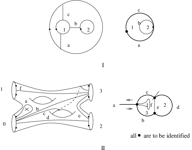
A number of operads of current interest [CS, J, V, MSS] are governed by a composition which, in effect, depends upon combining families of arcs in surfaces. Our operad composition on depends upon an explicit method of combining families of weighted arcs in surfaces, that is, each component arc of the family is assigned a positive real number; we next briefly describe this composition. Suppose that are surfaces with distinguished boundary components . Suppose further that each surface comes equipped with a properly embedded family of arcs, and let denote the arcs in which are incident on , for , as illustrated in part I of figure 1. Identify with to produce a surface . We wish to furthermore combine the arc families in to produce a corresponding arc family in , and there is evidently no well-defined way to achieve this without making further choices or imposing further conditions on the arc families (such as ).

I, arc families in two surfaces,\quaII, combining bands.
Our additional data required for gluing is given by an assignment of one real number, a weight, to each arc in each of the arc families. The weight on is interpreted geometrically as the height of a rectangular band whose core is identified with , for and . We shall assume that for simplicity, so that the total height of all the bands incident on agrees with that of ; in light of this assumption, the bands in can be sensibly attached along to the bands in along to produce a collection of bands in the surface as illustrated in part II of figure 1; notice that the horizontal edges of the rectangles decompose the rectangles into sub-rectangles and conversely. The resulting family of sub-bands, in turn, determines a weighted family of arcs in , one arc for each sub-band with a weight given by the width of the sub-band; thus, the weighted arc family in so produced depends upon the weights in a non-trivial but combinatorially explicit way. This describes the basis of our gluing operation on families of weighted arcs, which is derived from the theory of train tracks and partial measured foliations [PH]. In fact, the simplifying assumption that the total heights agree is obviated by considering not weighted families of arcs, but rather weighted families of arcs modulo the natural overall homothetic action of –so-called projectively weighted arc families; given projectively weighted arc families, we may de-projectivize in order to arrange that the simplifying assumption is in force (assuming that ), perform the construction just described, and finally re-projectivize. We shall prove in section 1 that this construction induces a well-defined operad composition on suitable classes of projectively weighted arcs.
The resulting operad structure provides a useful framework as is evidenced by the fact that there is an embedding of the cactus operad of Voronov [V] into this operad as a suboperad, as we discovered. This shows how to view the Chas–Sullivan [CS] string topology, which was the inspiration for our analysis and to which section 2 owes obvious intellectual gratitude, inside the combinatorial model. In particular, we recover in this way a surface description of the cacti which in turn can be viewed as a reduction of the surface structure in a very precise way. In fact, there is a reduction of any surface with arcs to a configuration in the plane, which is not necessarily a cactus and may have a much more complex structure. For the surfaces whose reduction is a cactus in the sense of [V], one retains the natural action on loop spaces by forgetting some of the internal topological structure of the surface but keeping an essential part of the information carried by the arcs. For more general configurations, a similar but more complicated structure is expected.
One virtue of viewing the cacti as a surface instead of as a singular level set is that in this way the branching behavior is nicely depicted while the “singularities of one–dimensional Feynman graphs do not appear” as Witten has pointed out many times. Furthermore, there are natural suboperads governing the Gerstenhaber and the BV structure, where the latter suboperad is generated by the former and the 1-ary operation of . On the level of homology, these operation just add one class, that of the BV operator. For cacti, the situation is much more complicated and is given by a bi–crossed product [K1].
It is conjectured [P1] that the full arc complex of a surface with boundary is spherical and thus will not carry much operadic information on the homological level. The sphericity of the full compactification can again be compared to the Deligne–Mumford situation where the compactification in the genus zero case leaves no odd cohomology and in a Koszul dual way is complementary to the gravity structure of the open moduli space. In general the idea of obtaining suboperads by imposing certain conditions can be seen as parallel to the philosophy of Goncharov–Manin [GM]. The Sphericity Conjecture [P1] would provides the basis for a calculation of the homology of the operads under consideration here, a task that will be undertaken in [KP].
One more virtue of having concrete surfaces is that we can also handle additional structures on the objects of the corresponding cobordism category, viz. the boundaries. We incorporate these ideas in the form of direct and semi–direct products of our operads with operads based on circles. These give geometrically natural extensions of the algebraic structure of BV algebras. This view is also inherent in [K1] where the cacti operads are decomposed into bi–crossed products. The operads built on circles which we consider have the geometric meaning of marking additional point in the boundary of a surface. Their algebraic construction, however, is not linked to their particular presentation but rather relies on the algebraic structures of as a monoid. They are therefore also of independent algebraic interest.
The paper is organized as follows: In section 1 we review the salient features of the combinatorial compactification of moduli spaces and the Sphericity Conjecture. Using this background, we define the operadic products on surfaces with weighted arcs that underlie all of our constructions. In section 2 we uncover the Gerstenhaber and Batalin–Vilkovisky structures of our operad on the level of chains with explicit chain homotopies. These chain homotopies manifestly show the symmetry of these equations. The BV–operator is given by the unique, up to homotopy, cycle of arc families on the cylinder. Section 3 is devoted to the inclusion of the cacti operad into the arc operad both in its original version [CS, V] as well as in its spineless version [K1]. This explicit map, called framing, also shows that the spineless cacti govern the Gerstenhaber structure while the Voronov cacti yield BV; this fact can also be read off from the explicit calculations of section 2 for the respective suboperads of , which are also defined in this section. The difference between the two sub–operads are operations corresponding to a Fenchel–Nielsen type deformation of the cylinder, i.e., the 1-ary operation of . A general construction which forgets the topological structure of the underlying surface and retains a collection of parameterized loops in the plane with incidence/tangency conditions dictated by the arc families is contained in section 4. Using this partial forgetful map we define the action of a suboperad of on loop spaces of manifolds. For the particular suboperads corresponding to cacti, this operation is inverse to the framing of section 3. In section 5 we define several direct and semi–direct products of our operad with cyclic and non–cyclic operads built on circles. One of these products yields for instance dGBV algebras. The operads built on circles which we utilize are provided by our analysis of this type of operad in the Appendix. The approach is a classification of all operations that are linear and local in the coordinates of the components to be glued. The results are not contingent on the particular choice of , but only on certain algebraic properties like being a monoid and are thus of a more general nature.
Acknowledgments The first author wishes to thank the IHÉS in Bures–sur–Yvette and the Max–Planck–Institut für Mathematik in Bonn, where some of the work was carried out, for their hospitality. The second author would like to thank USC for its hospitality. The financial support of the NSF under grant DMS#0070681 is also acknowledged by the first author as is the support of NATO by the second author.
1 The operad of weighted arc families in surfaces
It is the purpose of this section to define our basic topological operad. The idea of our operad composition on projectively weighted arc families was already described in the Introduction. The technical details of this are somewhat involved, however, and we next briefly survey the material in this section. To begin, we define weighted arc families in surfaces together with several different geometric models of the common underlying combinatorial structure. The collection of projectively weighted arc families in a fixed surface is found to admit the natural structure of a simplicial complex, which descends to a CW decomposition of the quotient of this simplicial complex by the action of the pure mapping class group of the surface. This CW complex had arisen in Penner’s earlier work, and we discuss its relationship to Riemann’s moduli space in an extended remark. The discussion in the Introduction of bands whose heights are given by weights on an arc family is formalized by Thurston’s theory of partial measured foliations, and we next briefly recall the salient details of this theory. The spaces underlying our topological operads are then introduced; in effect, we consider arc families so that there is at least one arc in the family which is incident on any given boundary component. In this setting, we define a collection of abstract measure spaces, one such space for each boundary component of the surface, associated to each appropriate projectively weighted arc family. We next define the operad composition of these projectively weighted arc families which was sketched in the Introduction and prove that this composition is well-defined. Our basic operads are then defined, and several extensions of the construction are finally discussed.
1.1 Weighted arc families
1.1.1 Definitions
Let be a fixed oriented topological surface of genus with punctures and boundary components, where , so the boundary of is necessarily non-empty by hypothesis. Fix an enumeration of the boundary components of once and for all. In each boundary component of , choose once and for all a closed arc , called a window, for each .
The pure mapping class group is the group of isotopy classes of all orientation-preserving homeomorphisms of which fix each pointwise (and fix each setwise), for each .
Define an essential arc in to be an embedded path in whose endpoints lie among the windows, where we demand that is not isotopic rel endpoints to a path lying in . Two arcs are said to be parallel if there is an isotopy between them which fixes each pointwise (and fixes each setwise) for .
An arc family in is the isotopy class of an unordered collection of disjointly embedded essential arcs in , no two of which are parallel. Thus, there is a well-defined action of on arc families.
1.1.2 Several models for arcs
We shall see that collections of arc families in a fixed surface lead to a natural simplicial complex, an open subset of which will form the topological spaces underlying our basic operads. Before turning to this discussion, though, let us briefly analyze the role of the windows in the definitions above and describe several geometric models of the common underlying combinatorics of arc families in bounded surfaces in order to put this role into perspective.

For the first such model, let us choose a distinguished point , for , and consider the space of all complete finite-area metrics on of constant Gauss curvature (so-called “hyperbolic metrics”) so that each is totally geodesic (so-called “quasi hyperbolic metrics”) on . To explain this, consider a hyperbolic metric with geodesic boundary on a once-punctured annulus and the simple geodesic arc in it asymptotic in both directions to the puncture; the induced metric on a component of gives a model for the quasi hyperbolic structure on near . The first geometric model for an arc family in is a set of disjointly embedded geodesics in , each component of which is asymptotic in both directions to some distinguished point ; see part II of figure 2.
In the homotopy class of each , there is a unique geodesic . Excising from any component which contains a point of , we obtain a hyperbolic structure on the surface with geodesic boundary (where in the special case of an annulus, collapses to a circle). Taking , we find a collection of geodesic arcs connecting boundary components (where in the special case of the annulus, we find two points in the circle).
This is our second geometric model for arc families. We may furthermore choose a distinguished point and a regular neighborhood of in , for . Provided , we may take sufficiently small that , so the arc forms a natural “window” containing . There is then an ambient isotopy of which shrinks each window down to a small arc , under which is transported to a family of (non-geodesic) arcs with endpoints in the windows . In case does lie in , then let us simply move a small amount in the direction of the natural orientation (as a boundary component of ) along and perform the same construction; see part III of figure 2.
This leads to our final geometric model of arc families, namely, the model defined in 1.1.1 for the purposes of this paper, of arcs in a bounded surface with endpoints in windows. This third model is in the spirit of train tracks and measured foliations (cf. [PH]) as we shall see and is most convenient for describing the operadic structure.
1.1.3 The arc complex
Let us inductively build a simplicial complex as follows. For each singleton arc family in , there is a distinct vertex of . Having thus inductively constructed the -skeleton of for , let us add a -simplex to for each arc family in of cardinality . The simplicial structure on itself is the natural one, where faces correspond to sub-arc families of , and we may therefore identify the proper faces of with simplices in the -skeleton of . Adjoining -simplices in this manner for each such arc family of cardinality defines the -skeleton of . This completes the inductive definition of the simplicial complex .
is thus a simplicial complex, upon which acts continuously, and we define the quotient topological space to be . If , then the arcs come in a canonical linear ordering. Namely, the orientation of induces an orientation on each window, and traversing the windows in the order in these orientations, one first encounters an endpoint of the arcs in some order, which prescribes the claimed linear ordering. Thus, cells in cannot have finite isotropy in , and the simplicial decomposition of descends to a CW decomposition of itself.
1.1.4.
Sphericity Conjecture\qua[P1]\quaFix any surface with . Then is piecewise-linearly homeomorphic to a sphere of dimension .
Recent work seems to provide a proof of this conjecture at least in the case of planar surfaces as will be taken up elsewhere. It is worth emphasizing that the current paper is independent of the Sphericity Conjecture, but this gives a useful perspective on the relationship between Riemann’s moduli space and the operads studied here.
1.1.5.
Remark\qua It is the purpose of this remark to explain the geometry underlying which was uncovered in [P1, P2]. Recall the distinguished point chosen in our second geometric model for arc families. The “moduli space” of the surface with boundary is the collection of all complete finite-area metrics of constant Gauss curvature -1 with geodesic boundary, together with a distinguished point in each boundary component, modulo push forward by diffeomorphisms. There is a natural action of on by simultaneously scaling each of the hyperbolic lengths of the geodesic boundary components, and we let denote the quotient. The main result of [P2] is that is proper homotopy equivalent to the complement of a codimension-two subcomplex of , where corresponds to arc families so that some component of is other than a polygon or once-punctured polygon. It is remarkable to suggest that by adding to a space homotopy equivalent to a suitable simplicial complex we obtain a sphere. There is much known [P1] about the geometry and combinatorics of and . Furthermore, the Sphericity Conjecture should be useful in calculating the homological operads of the arc operads.
1.1.6 Notation
We shall always adopt the notation that if is the -orbit of an arc family in , then denotes some chosen arc family representing . Furthermore, it will sometimes be convenient to specify the components , for , of an arc family representing , and we shall write simply in this case. Since the linear ordering on components of is invariant under the action of , it descends to a well-defined linear ordering on the components underlying the -orbit .
Of course, a -dimensional cell in the CW decomposition of is determined by the -orbit of some arc family , and (again relying on the -invariant linear ordering discussed previously) a point in the interior of this cell is determined by the projective class of a corresponding -tuple of positive real numbers. As usual, we shall let denote affine coordinates on the projective classes of corresponding non-negative real -tuples, and if , for in a proper subset , then the point of corresponding to is identified with the point in the cell corresponding to with projective tuple gotten by deleting all zero entries of .
To streamline the notation, if is in and if is an assignment of numbers, called weights, one weight to each component of , then we shall sometimes suppress the weights by letting denote the arc family with corresponding weights . In the same manner, the projectivized weights on the components of will sometimes be suppressed, and we let denote the arc family with projective weights . These same notations will be used for -classes of arc families as well, so, for instance, denotes the -orbit with weights , and a point in may be denoted simply , where the projective weight is given by .
1.2 Partial measured foliations
Another point of view on elements of , which is useful in the subsequent constructions, is derived from the theory of “train tracks” (cf. [PH]) as follows. If is given weights , then we may regard as a transverse measure on , for each to determine a “measured train track with stops” and corresponding “partial measured foliation”, as considered in [PH].
For the convenience of the reader, we next briefly recall the salient and elementary features of this construction. Choose for the purposes of this discussion any complete Riemannian metric of finite area on , suppose that each is smooth for , and consider for each the “band” in consisting of all points within -distance of . If it is necessary, scale the metric to , for , to guarantee that these bands are embedded, pairwise disjoint in , and have their endpoints lying among the windows. The band about comes equipped with a foliation by the arcs parallel to which are a fixed -distance to , and this foliation comes equipped with a transverse measure inherited from ; thus, is regarded as a rectangle of width and some irrelevant length, for . The foliated and transversely measured bands , for combine to give a “partial measured foliation” of , that is, a foliation of a closed subset of supporting an invariant transverse measure (cf. [PH]). The isotopy class in rel of this partial measured foliation is independent of the choice of metric .
Continuing to suppress the choice of metric , for each , consider , which is empty if does not meet and is otherwise a collection of closed intervals in with disjoint interiors. Collapse to a point each component complementary to the interiors of these intervals in to obtain an interval, which we shall denote . Each such interval inherits an absolutely continuous measure from the transverse measures on the bands.
1.2.1.
Definition\quaGiven two representatives and of the sameweighted -orbit , the respective measure spaces and are canonically identified, which allows us to consider the measure space of a weighted -orbit itself, which is called the end of , for each .
1.3 The spaces underlying the topological operad
1.3.1 Definitions
An arc family in is said to be exhaustive if for each boundary component , for , there is at least one component arc in with its endpoints in the window . Likewise, a -orbit of arc families is said to be exhaustive if some (that is, any) representing arc family is so. Define the topological spaces
which are the spaces that comprise our various families of topological operads. In light of Remark 1.1.5, is identified with an open subspace of properly containing a space homotopy equivalent to , and is spherical in at least the planar case.
Enumerating the boundary components of as once and for all (where will play a special role in the subsequent discussion) and letting denote the symmetric group, there is a natural -action on the labeling of boundary components which restricts to a natural -action on the boundary components labeled . Thus, and act on , and extending by the diagonal action of on , the symmetric groups and likewise act on , where by definition acts trivially on the first coordinate in .
Continuing with the definitions, if , let us choose a corresponding deprojectivization , fix some boundary component , for , and let denote the total measure. There is then a unique orientation-preserving mapping
| (1) |
which maps the (class of the) first point of in the orientation of the window to , where the measure on the domain is and on the range is the Haar measure on . Of course, each is injective on the interior of while . Furthermore, if and are two different deprojectivizations of a common projective class, then extends continuously to the identity on .
1.3.2.
Remark\qua We do not wish to specialize to one or another particular case at this stage, but if comes equipped with an a priori absolutely continuous measure (for instance, if comes equipped with a canonical coordinatization, or if or comes equipped with a fixed Riemannian metric), then we can identify with , for each , in the obvious manner (where, if the a priori total measure of is , then we alter the Riemannian metric employed in the definition of the bands so that the total measure agrees with for each and finally collapse the endpoints of to a single point).
Thus, the idea is that the end of gives a model or coordinatization for , but of course, altering the underlying in turn alters the coordinatization of . The trivial product leads in this way to a family of coordinatizations of which are twisted by .
1.3.3 Pictorial representations of arc families
As explained before, there are several ways in which to imagine weighted arc families near the boundary. They are illustrated in figure 2. It is also convenient, to view arcs near a boundary component as coalesced into a single wide band by collapsing to a point each interval in the window complementary to the bands; this interval model is illustrated in figure 3, part I. It is also sometimes convenient to further take the image under the maps 1 to produce the circle model as is depicted in figure 3, part II.

1.4 Gluing arc families
1.4.1 Gluing weighted arc families
Given two weighted arc families in and in so that , for some , we shall next make choices to define a weighted arc family in as follows.
First of all, let denote the boundary components of , let denote the boundary components of , and fix some index . Each boundary component inherits an orientation in the standard manner from the orientations of the surfaces, and we may choose any orientation-preserving homeomorphisms and each of which maps the initial point of the respective window to the base-point . Gluing together and by identifying with if produces a space homeomorphic to , where the two curves and are thus identified to a single separating curve in . There is no natural choice of homeomorphism of with , but there are canonical inclusions and .
We enumerate the boundary components of in the order
and re-index letting , for , denote the boundary components of in this order. Likewise, first enumerate the punctures of in order and then those of to determine an enumeration of those of , if any. Let us choose an orientation-preserving homeomorphism which preserves the labeling of the boundary components as well as those of the punctures, if any.
In order to define the required weighted arc family, consider the partial measured foliations in and in corresponding respectively to and . By our assumption that , we may produce a corresponding partial measured foliation in by identifying the points and if . The resulting partial measured foliation may have simple closed curve leaves which we must simply discard to produce yet another partial measured foliation in . The leaves of thus run between boundary components of and therefore, as in the previous section, decompose into a collection of bands of some widths , for . Choose a leaf of in each such band and associate to it the weight given by the width of to determine a weighted arc family in which is evidently exhaustive. Let denote the image in under of this weighted arc family.
1.4.2.
Lemma\quaThe -orbit of is well-defined as varies over a -orbit of weighted arc families in and varies over a -orbit of weighted arc families in .
Proof.
Suppose we are given weighted arc families , for , and , for , as well as a pair of homeomorphisms as above together with the pairs and of induced inclusions, for . Let denote the partial measured foliations and let and denote the corresponding weighted arc families in and , respectively, constructed as above from and , for .
Let , and remove a tubular neighborhood of in to obtain the subsurface , for . Isotope off of in the natural way to produce inclusions and with disjoint images, for .
induces a homeomorphism supported on so that , and induces a homeomorphism supported on so that . Because of their disjoint supports, and combine to give a homeomorphism so that and . We may extend by any suitable homeomorphism to produce a homeomorphism .
By construction and after a suitable isotopy, maps to , and there is a power of a Dehn twist along supported on the interior of so that also maps to . thus maps to and hence to . It follows that the homeomorphism
maps to , so and are indeed in the same -orbit.∎
1.4.3.
Remark\qua It is worth emphasizing again that, owing to the dependence upon weights, the arcs in are not simply determined just from the arcs in and ; the arcs in depend upon the weights. It is also worth pointing out that the composition just described is not well-defined on projectively weighted arc families but only on pure mapping class orbits of such. In fact, by making choices of standard models for surfaces as well as standard inclusions of these standard models, one can lift the composition to the level of projectively weighted arc families.
1.4.4.
Remark\qua We simply discard simple closed curve components which may arise in our construction, and J L Loday has proposed including them here in analogy to [J]. In fact, they naturally give rise to the conjugacy class of an element of the real group ring of the fundamental group of .
1.4.5.
Definition\quaGiven and and an index , let us choose respective deprojectivizations and and write the weights
Define
where in each sum the weights are taken with multiplicity, e.g., if has both endpoints at , then there are two corresponding terms in .
Since both arc families are exhaustive, , and we may re-scale
so that the entry of agrees with the entry of .
1.4.6 A pictorial representation of the gluing
A graphical representation of the gluing can be found in figure 4, where we present the gluing in three of the different models. More examples of gluing in the interval and circle models can be found in figure 15 and throughout the later sections.

1.5 The basic topological operads
1.5.1.
Definition\quaFor each , let (where the “” stands for compact planar), and furthermore, define the direct limit of as under the natural inclusions.
1.5.2.
Theorem\quaThe compositions of Definition 1.4.5 imbue the collection of spaces with the structure of a topological operad under the natural –action on labels on the boundary components. The operad has a unit given by the class of an arc in the cylinder meeting both boundary components, and the operad is cyclic for the natural –action.
Proof.
The first statement follows from the standard operadic manipulations. The second statement is immediate from the definition of composition. For the third statement, notice that the composition treats the two surfaces symmetrically, and the axiom for cyclicity again follows from the standard operadic manipulations.∎
In precisely the same way, we have the following theorem.
1.5.3.
Theorem\quaThe composition of Definition 1.4.5 induces a composition on which imbues this collection of spaces with the natural structure of a cyclic topological operad with unit.
1.5.4 The deprojectivized spaces
For the following it is convenient to introduce deprojectivized arc families. This amounts to adding a factor for the overall scale.
Let be the space of weighted arc families; it is clear that is homotopy equivalent to .
As the definition 1.4.5 of gluing was obtained by lifting to weighted arc families and then projecting back, we can promote the compositions to the level of the spaces . This endows the spaces with a structure of a cyclic operad as well. Moreover, by construction the two operadic structures are compatible. This type of composition can be compared to the composition of loops, where such a rescaling is also inherent. In our case, however, the scaling is performed on both sides which renders the operad cyclic.
In this context, the total weight at a given boundary component given by the sum of the individual weights of incident arcs makes sense, and thus the map 1 can be naturally viewed as a map to a circle of radius .
1.6.
Notation\quaWe denote the operad on the collection of spaces by and the operad on the collection of spaces by . By an “Arc algebra”, we mean an algebra over the homology operad of . Likewise, and are comprised of the spaces and respectively, and an “Arccp algebra” is an algebra over the homology of
1.6.1.
Remark\qua In fact, the restriction that the arc families under consideration must be exhaustive can be relaxed in several ways with the identical definition retained for the composition. For instance, if the projectively weighted arc family fails to meet the boundary component and , then we can set to be regarded as an arc family in , where the boundary components have been re-labeled.
In both formulations, we must require that in order that is non-empty, but this asymmetric treatment destroys cyclicity.
Another possibility is to include the empty arc family in the operad as any arc family with all weights zero to preserve cyclicity. The composition then imbues the deprojectivized themselves with the structure of a topological operad, but the corresponding homology operad, in light of the Sphericity Conjecture 1.1.4 would be trivial i.e., the trivial one-dimensional –module for each .
1.6.2 Turning on punctures and genus
When allowing genus or the number of punctures to be different from zero, there are two operators for the topological operad that generate arc families of all genera respectively with any number of punctures from arc families of genus zero with no punctures. These operators are depicted in figure 5.

For the corresponding linear homology operad, we expect similarities with [LM], in which the punctures play the role of the second set of points. This means that the linear operad will act on tensor powers of two linear spaces, one for the boundary components and one for the punctures. In this extension of the operadic framework, there is no gluing on the punctures and the respective linear spaces should be regarded as parameterizing deformations which perturb each operation separately.
1.6.3 Other Props and Operads
There are related sub-operads and sub-props of other than and which are of interest. In the general case, one may specify a symmetric -by- matrix as well as an -vector of zeroes and ones over and consider the subspace of where arcs are allowed to run between boundary components and if and only if and are required to meet boundary component if and only if . For instance, the case of interest in this paper corresponds to the matrix and the vector whose entries are all one. In Remark 1.6.1, we also mentioned the example with the matrix consisting entirely of entries one and the standard first unit basis vector.
For a class of examples, consider a partition of , into “inputs” and “outputs”, where if and only if and are each singletons, and is the vector whose entries are all one. The corresponding prop is presumably related to the string prop of [CS].
There are many other interesting possibilities. For instance, the cacti operad of [V] and the spineless cacti of [K1] will be discussed and studied in sections 2 and 3, and other related cactus-like examples are studied in [K1]. A further variation is to stratify the space by incidence matrices with non–negative integer entries corresponding to the number of arcs at each boundary component.
2 The Gerstenhaber and BV structure of
In this section we will show that there is a structure of Batalin-Vilkovisky algebra on Arc algebras and Arccp algebras. More precisely, any algebra over the singular chain complex operad or is a BV algebra up to certain chain homotopies. For convenience, will denote or , since for our calculations, we only require . An element in will be also called an arc family. We shall realize the underlying surfaces in the plane with the boundary being the outside circle. The conventions we use for the drawings is that all circles are oriented counterclockwise. Furthermore if there is only one marked point on the circle, it is the beginning of the window. If there are two marked points on the boundary, the window is the smaller arc between the two.
Via gluing, any arc family in gives rise to an n–ary operation on arc families in . Here one has to be careful with the parameterizations. To be completely explicit we will always include them if we use a particular family as an operation.
As mentioned in the Introduction, many of the calculations of this section are inspired by [CS].
2.1 A reminder on some algebraic structures
In this section, we would like to recall some basic definitions of algebras and their relations which we will employ in the following. The proofs in this subsection are omitted, since they are straightforward computations. They can be found in [G, Ge].
2.1.1.
Definition\qua(Gerstenhaber)\quaA pre–Lie algebra is a graded vector space together with a bilinear operation that satisfies
Here denotes the degree of .
2.1.2.
Definition\quaAn odd Lie algebra is a graded vector space together with a bilinear operation which satisfies
2.1.3.
Remark\quaPre–Lie algebras of the above type are sometimes also called right symmetric algebras. There is also the notion of a left symmetric algebra, which satisfies
Given a left symmetric algebra its opposite algebra is right symmetric and vice–versa. Here the multiplication for the opposite algebra is . Hence it is a matter of taste, which algebra type one regards. To match with string topology, one has to use left symmetric algebras, while to match with the Hochschild cochains, one will have to use right symmetric algebras.
2.1.4.
Definition\quaA Gerstenhaber algebra or an odd Poisson algebra is a graded, graded–commutative associative algebra endowed with an odd Lie algebra structure which satisfies the compatibility equation
2.1.5.
Proposition\qua(Gerstenhaber)\quaFor any pre-Lie algebra , the bracket defined by
| (2) |
endows with a structure of odd Lie algebra.
2.1.6.
Remark\quaThe same holds true for a right symmetric algebra.
2.1.7.
Definition\quaA Batalin–Vilkovisky (BV) algebra is an associative super–commutative algebra together with an operator of degree that satisfies
Here super–commutative means as usual graded commutative, i.e. .
2.1.8.
Proposition\qua(Getzler)\quaFor any BV–algebra define
| (3) |
Then is a Gerstenhaber algebra.
2.1.9.
Definition\quaWe call a triple a GBV–algebra if is a BV algebra and satisfies the equation (3). By the Proposition above is a Gerstenhaber algebra.
The purpose of this definition is that in some cases as in the case of the Arc operad it happens that a bracket as well as the BV operator appear naturally. In our case the bracket comes naturally from a pre–Lie structure which one can also view as a product, while the BV operator appears from a cycle naturally parameterized by . We use the name GBV algebra to indicate that these structures although having independent origin are indeed compatible. As we will show below, the independent origin can be interpreted as saying that the Gerstenhaber structure is governed by one suboperad and the BV–structure by another bigger suboperad which contains the previous one. Moreover the bracket of the BV structure coincides with the bracket of the Gerstenhaber structure already present in the smaller suboperad.
2.2 Arc families and their induced operations
The points in are parameterized by the circle, which is identified with , where is identified to . To describe a parameterized family of weighted arcs, we shall specify weights that depend upon the parameter . Thus, by taking figure 6 describes a cycle that spans .

As stated above, there is an operation associated to the family . For instance, if is any arc family , is the family parameterized by with the map given by the picture by inserting into the position 1. By definition,
In we have the basic families depicted in figure 7 which in turn yield operations on .

To fix the signs, we fix the parameterizations we will use for the glued families as follows: say the families are parameterized by and and . Then is the family parameterized by as defined by figure 7 (i.e., the arc family inserted in boundary and the arc family inserted in boundary ).
Interchanging labels 1 and 2 and using as a chain homotopy as in figure 8 yields the commutativity of up to chain homotopy
| (4) |
Notice that the product is associative up to chain homotopy.
Likewise is defined to be the operation given by the second family of figure 7 with parameterized over .
By interchanging the labels, we can produce a cycle as shown in figure 8 where now the whole family is parameterized by .

2.2.1.
Definition\quaWe have defined the following elements in :
and in ;
in , which is commutative and associative up to a boundary.
and in with and .
Note that and are cycles, whereas is not.
2.2.2.
Remark\quaWe would like to point out that the symbol in the standard super notation of odd Lie brackets , which is assigned to have an intrinsic degree of 1, corresponds geometrically in our situation to the one–dimensional interval .
2.3 The BV operator
The operation corresponding to the arc family is easily seen to square to zero in homology. It is therefore a differential and a natural candidate for a derivation or a higher order differential operator. It is easily checked that it is not a derivation, but it is a BV operator, as we shall demonstrate.
It is convenient to introduce the family of operations on arc families which are defined by figure 9, where the families are parameterized over .

We notice the following relations which are the raison d’être for this definition:
| (5) | |||||
| (6) |
where is the cyclic permutation and is the standard supersign of the permutation. The homotopy here is just a reparameterization of the variable .
There is a further relation immediate from the definition which shows that the only “new” operation is
| (7) |
where we use a homotopy to scale all weights of the bands not hitting the boundary 1 to the value 1.
2.3.1.
Lemma\qua
| (8) |
Proof.
The proof is contained in figure 10. Let , and , be arc families then the two parameter family filling the square is parameterized over . This family gives us the desired chain homotopy.∎

2.3.2.
Proposition\quaThe operator satisfies the relation of a BV operator up to chain homotopy.
| (9) | |||||
Thus, any Arc algebra and any Arccp algebra is a BV algebra.
Proof.
The proof follows algebraically from Lemma 2.3.1 and equation (2.3). We can also make the chain homotopy explicit. This has the advantage of illustrating the symmetric nature of this relation in directly.
Given arc families , and , we define the two parameter family defined by the figure 11 where the families in the rectangles are the depicted two parameter families parameterized over and the triangle is not filled, but rather its boundary is the operation .

From the diagram we get the chain homotopy consisting of three, and respectively twelve, terms.
| (10) | |||||
2.4 Gerstenhaber Structure
We have already defined the operation whose odd commutator is given by the BV operator.
2.4.1.
Theorem\quaThe Gerstenhaber bracket induced by is given by the operation
In other words is a GBV–Algebra up to homotopy.

Proof.
We consider the arc family depicted in figure 12, where the two parameter arc families are parameterized via , where is the triangle with induced orientation, and where the middle loop is suitably re–parameterized. Inserting in the boundary 1, and in boundary 2, and passing to homology, we can read off the relation:
or with :
2.4.2.
Remark\quaAlgebraically, the Jacobi identity and the derivation property of the bracket follow from the BV relation. For the less algebraically inclined we can again make everything topologically explicit. This also has the virtue of showing how different weights contribute to topologically distinct gluings. This treatment also shows that we can restrict ourselves to the case of linear (Chinese) trees of section 3 or to cacti without spines (cf. section 5 and [K1]) and therefore have a Gerstenhaber structure on this level.
2.4.3 The associator
It is instructive to do the calculation in the arc family picture with the operadic notation. For the gluing we obtain the elements in presented in figure 13 to which we apply the homotopy of changing the weight on the boundary 3 from 2 to 1 while keeping everything else fixed. We call this normalization.

Unraveling the definitions for the normalized version yields figure 14, where in the different cases the gluing of the bands is shown in figure 15.

The gluing in arc families is simpler and yields the gluing depicted in figure 16 to which we apply a normalizing homotopy — by changing the weights on the bands emanating from boundary 1 from the pair to using pointwise the homotopy for :
Combining figures 14 and 16 while keeping in mind the parameterizations we can read off the pre–Lie relation:
| (11) |
which shows that the associator is symmetric in the first two variables and thus following Gerstenhaber [G] we obtain:
2.4.4.
Corollary\qua The bracket satisfies the odd Jacobi identity.
2.4.5 The Gerstenhaber structure
The derivation property of the bracket follows from the compatibility equations which are proved by the relations represented by the two diagrams 17 and 18. The first case is just a calculation in the arc family picture. In the second case the arc family picture also makes it very easy to write down the family inducing the chain homotopy explicitly. We fix arc families parameterized over respectively.


First notice that the family parameterized by , which is depicted in figure 17, illustrates that

Second, the special two parameter family shown in figure 18 –where the two parameter arc family realizing the chain homotopy is parameterized over with – gives the chain homotopy
In both cases, we used normalizing homotopies as before.

These two equations imply that
| (12) |
and we obtain:
2.4.6.
Proposition\quaThe bracket is a Gerstenhaber bracket up to chain homotopy on or for the product .
Summing up, we obtain:
2.5.
Theorem\quaThere is a BV structure on or up to explicit chain boundaries. The induced Gerstenhaber bracket is also given by such explicit boundaries. This bracket is compatible with a product (associative and commutative up to explicit boundaries) given by a point in .
2.6.
Corollary\quaAll Arccp and Arc algebras are Batalin-Vilkovisky algebras. The Gerstenhaber structure induced by the BV operator coincides with the bracket induced by the pre–Lie product . Hence all Arccp and Arc algebras are GBV algebras.
3 Cacti as a suboperad of
In the last section (section 2), we exhibited a GBV structure up to chain homotopy on . Inspecting the arc families realizing the relevant homotopies, we observe that the Gerstenhaber structure is already present in a suboperad which we shall discuss here. This suboperad, called “linear trees”, corresponds to the “spineless cacti” of [K1]. Furthermore for the BV operator, we only need to add the one more operation , so that the BV structure is realized on the suboperad generated by spineless cacti and . Lastly the suboperad generated by spineless cacti is contained in the suboperad generated by cacti and the two Gerstenhaber structures agree, i.e. the one coming from the BV operator and the previously defined bracket.
We will furthermore show that this operad is the image of an embedding (up to homotopy) of Voronov cacti [V] into .
By the results of [CS, V], algebras over the cacti operad have a BV structure. The map of operads we construct will thus induce the structure of BV algebras for algebras over the homology of . This induced structure is indeed the same as that defined in section 2 as can be seen from the embedding and our explicit realization of all relevant operations.
3.1 Suboperads
3.1.1.
Definition\quaThe trees suboperad is defined for arc families in surfaces with in the notation of 1.6.3 by the allowed incidence matrix , whose non–zero entries are , for , and required incidence relations , whose entries are all equal to one.
This is a suboperad of , and a representation of it as a collection of labeled trees can be found in [K1].
Dropping the requirement that , we obtain a suboperad of called the rooted graphs or Chinese trees suboperad.
3.1.2.
Remark\quaWe have already observed that there is a linear and — by forgetting the starting point — a cyclic order on the set of arcs incident on each boundary component. In the (Chinese) trees suboperad all bands must hit the –th component, which induces a linear and a cyclic order on all of the bands. Furthermore the cyclic order is “respected” for trees, in the sense that the bands meeting the –th component form a cyclic subchain in the cyclic order of all bands, for Chinese trees, this is an extra condition. And again all Chinese trees which satisfy this condition form a suboperad which we call the cyclic Chinese trees. The linear order is, however, not even respected for trees, as can easily be seen in .
3.1.3.
Linearity Condition\quaWe say that an element of the (cyclic Chinese) trees suboperad satisfies the Linearity Condition if the linear orders match, i.e., the bands hitting each boundary component in their linear order are a subchain of all the bands in their linear order derived from the –th boundary.
It is easy to check that this condition is stable under composition.
We call the suboperad of elements satisfying the Linearity Condition of the (cyclic Chinese) trees operad the (cyclic Chinese) linear trees operad.
3.1.4.
Proposition\quaThe suboperad generated by (cyclic Chinese) linear trees and inside coincides with (cyclic Chinese) trees.
Proof.
Given a (Chinese) tree we can make it linear by gluing on twists from at the various boundary components as these twists have the effect of moving the marked point of the boundary around the boundary. Since the cyclic order is already respected, such twists may be applied to arrange that the linear orders agree. Since (Chinese) linear trees and lie inside the (Chinese) trees operad the reverse inclusion is obvious. ∎
3.2 Cacti
There are several species of cacti, which are defined in [K1], to which we refer the reader for details. By cacti, we mean Voronov cacti as defined in [V], i.e., as connected, planar tree-like configurations of parameterized loops, together with a marked point on the configuration. This point, called “global zero”, defines an outside circle or perimeter by taking it to be the starting point and then going around all loops in a counterclockwise fashion by jumping onto the next loop (in the induced cyclic order) at the intersection points. The spineless variety of cacti is obtained by postulating that the local zeros defined by the parameterizations of the loops coincide with the first intersection point of the perimeter with a loop (sometimes called a “lobe”) of the cactus.
The gluing of two cacti and is done by first scaling in such a way that the length of i–th lobe of matches the length of the outside circle of and then inserting the cactus into the i–th lobe by using the parameterization as gluing data.
3.2.1 Scaling of a cactus
Cacti and spineless cacti both come with a universal scaling operation of which simultaneously scales all radii by the same factor . This action is a free action and the gluing descends to the quotient by this action.
3.2.2 Left, Right and Symmetric Cacti
For the operadic gluings one has three basic possibilities to scale in order to make the size of the outer loop of the cactus that is to be inserted match the size of the lobe into which the insertion should be made.
- 1.
Scale down the cactus which is to be inserted. This is the original version – we call it the right scaling version.
- 2.
Scale up the cactus into which will be inserted. We call it the left scaling version.
- 3.
Scale both cacti. The one which is to be inserted by the size of the lobe into which it will be inserted and the cactus into which the insertion is going to be taking place by the size of the outer loop of the cactus which will be inserted. We call this it the symmetric scaling version.
All of these versions are of course homotopy equivalent and in the quotient operad of by overall scalings, the projective cacti they all descend to the same glueing.
3.2.3 Framing of a spineless cactus
We will give a map of spineless cacti into called a framing. First notice that a spineless cactus can be decomposed by the initial point and the intersection points into a sequence of arcs following the natural orientation given by the data. These arcs are labeled by their lengths as parts of parameterized unit circles. To frame a given spineless cactus, draw a pointed circle around it and run an arc from each arc of the cactus to the outside circle respecting the linear order, starting with the initial arc of the cactus as the first arc emanating from the outside circle in its orientation. Label each such arc by the parameter associated to the arc of the cactus.
We can think of attaching wide bands to the arc of the cactus. The widths of the bands are just the lengths of the arcs to which they are attached. Using these bands we identify the outside circle with the circumference of the cactus. Notice that this “outside” circle appears in the gluing formalism for cacti (see figures 19 to 22).
3.2.4.
Proposition\qua The operation of framing gives a map of operads of spineless cacti into whose image lies in the linear trees suboperad. Moreover we have a commutative square
where is defined by taking any lift of a spineless cactus/ to spineless cacti. The map becomes an operadic map, if one uses the symmetric glueing for cacti.
Proof.
It is obvious that the image of the framing of spineless cacti lies inside the linear trees suboperad. It is also clear that two cacti which differ by a scaling of the type 3.2.1 get mapped to the same arc family, so that the framing factors through spineless cacti modulo . The gluings for cacti and arc families are equivariant with respect to framing, as is obvious from the point of view of identifying the outside circle with the circumference of a cactus. By considering weights rather than projective weights on the arcs of a framing of a cactus, we can lift the framing of a cactus to . ∎
To illustrate this map we will provide several examples.
3.2.5 The basic operations of spineless cacti and their images
The operations: id, dot and are pictured in figure 19 as well as their images. This accounts for all 1 and 2 boundary cacti up to an overall normalization.
The generic cacti and their images are presented in figures 20 and 21. All degenerate configurations are contained in the examples of figure 21.


3.2.6.
Example\quaAs a benefit, an example of a framing of a four boundary cactus is included in figure 22.

3.3 Framing of a cactus
We wish to conclude this section with the framing procedure for cacti. It is essentially the same as for spineless cacti. We decompose the cactus into the arcs of its perimeter, where the break point of a cactus with spines are the intersection points, the global zero and the local zeros. One then runs an arc from each arc to an outside pointed circle which is to be drawn around the cactus configuration. The arcs should be embedded starting in a counterclockwise fashion around the perimeter of the circle. The marked points on the inside boundaries correspond to the local zeros of the inside circles viz. lobes of the cactus.
Two examples of this procedure are provided in figure 23.

Analogously to Proposition 3.2.4 we have:
3.3.1.
Proposition\quaThe operation of framing gives a map of operads of cacti into whose image lies in the trees suboperad. Moreover we have a commutative square
where is defined by taking any lift of a cactus/ to cacti and we again regard symmetric glueing for cacti.
3.4.
Remark\quaIn the previous section, the arc families we employed to provide the homotopies to exhibit the GBV structure had another common characteristic: their total weights at all boundary components except at the –th boundary component were all equal (to one). This property is not stable under gluing though. However, one can define a quasi–operad of normalized cacti [K1], where a quasi–operad is an operad which is not necessarily associative. Spineless cacti are however homotopy associative as an operad and moreover there is a chain decomposition for spineless cacti whose cellular chains give an honest operad under the induced compositions [K1]. Furthermore this cellular operad gives a solution to Deligne’s conjecture on the Hochschild cohomology of an associative algebra [K2]. Under framing normalized spineless cacti are a quasi–suboperad up to homotopy, i.e., the glueings are not equivariant, but are equivariant up to homotopy. In fact in [K1] it is shown that (spineless) cacti are the direct product of normalized (spineless) cacti and a scaling operad built on , and moreover all structures such as the Gerstenhaber and BV can be defined on the level of normalized cacti.
4 The Loop of an arc family
Given a surface with arcs we can forget some of the structure and in this way either produce a collection of loops or one loop which is given by using the arcs as an equivalence relation. Using these two maps we obtain an operation of the Chinese trees suboperad of on the loop space of any manifold on the homological level.
We expect that this action can be enlarged to all of , but for this we would need a generalization of the results of Cohen and Jones [CJ], which we intend to study elsewhere.
4.0.1 The boundary circles
Given an exhaustive weighted arc family in the surface , we can consider the measure-preserving maps
| (13) |
where is a circle of radius and is the total weight of the arc family at the –th boundary. Combining these maps, we obtain
| (14) |
Choosing a measure on as in section 1 to identify with , we finally obtain a map
| (15) |
Notice that the image of the initial points of the bands give well-defined basepoints for each .
4.1 The equivalence relations induced by arcs
On the set there is a natural reflexive and symmetric relation given by if and are on the same leaf of the partial measured foliation.
4.2.
Definition\quaLet be the equivalence relation on generated by . In other words if there are leaves , for , so that and .
4.2.1.
Remark\quaIt is clear that neither the image of — which will denote by — as a collection of parameterized circles nor the relation depends upon the choice of measure on .
4.3.
Definition\quaGiven a deprojectivized arc family , we define and denote the projection map .
Furthermore, we define two maps taking values in the monoidal category of pointed spaces:
| (16) | |||||
| (17) |
and call them the internal and external loops of in . We denote the space with induced topology given by the collection of images of all by .
Notice that there are marked points on for
Examples of loops of an arc family are depicted in figures 24–26. In figure 26 I the image of the boundary 1 runs along the outside circle and then around the inside circle. The same holds for the boundary 3 in figure 26 II. In both 26 I and II, the outside circle and its basepoint are in bold.

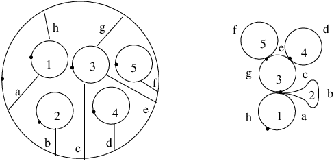
4.3.1.
Remark\quaThere are two types of intersection points for pairs of loops. The first are those coming from the interiors of the bands; these points are double points and occur along entire intervals. The second type of multiple point arises from the boundaries of the bands via the transitive closure; they can have any multiplicity but are isolated.
4.4 From loops to arcs
If the underlying surface of an arc family satisfies , then its Loop together with the parameterizations uniquely determines the arc family. In other words, the map is a section of .
4.4.1.
Definition\quaA configuration of circles is the image of a surjection of metric spaces such that each point of lies in the image of at least two components and the intersections of the images of more than two components are isolated. Let be the space of all such configurations of circles with the natural topology. We call a configuration of circles planar, if can be embedded in the plane with the natural orientation for all images coinciding with the induced orientation and the opposite orientation for . We call the space of planar configurations of circles .
4.4.2.
Proposition\quaThe map is surjective.
Proof.
To describe a right inverse, fix , fix an embedding of and in the plane, fix an identification of each boundary component with , and identify the disjoint union of these boundary components regarded as labeled circles with the source of . On , remove the images of the basepoints. For each component of dimension one in the intersection of two of the components of the map , draw an arc between the respective boundaries on of width given by the length of that component. These arcs are to be embedded in the linear order dictated by the various parameterizations and incidence conditions in the plane. If it happens in this way that an arc arises that is parallel to the boundary, then we insert a puncture in the region between the arc and the respective boundary. Since the higher order intersections are isolated they do not contribute. It is easily checked that this yields a right inverse of Loop. ∎
4.4.3.
Proposition and Definition\quaThe deprojectivized arc families such that constitute a suboperad of . We call this suboperad .
4.4.4.
Proposition\quaIf then is a cactus. Furthermore, the operad is identical to the operad of Chinese trees.
Proof.
If , then there are no arcs running between two boundary components if neither is . Furthermore, since , there is no arc running from to .∎
Collecting the results above, we have shown:
4.5.
Theorem\quaThe framing of a cactus is a section of and is thus an embedding. This embedding identifies (normalized and/or spineless) cacti as (normalized and/or linear) trees.
where is defined by choosing any lift and the glueing for cacti is the symmetric glueing.
4.6 Comments on an action on the loop space
Given a manifold we can consider its loop space . Using the configuration we have maps
| (18) |
where are continuous maps of the images of the configurations into , i.e., such a map takes a configuration and produces a continuous ; the maps are given by and .
One would like to follow the Pontrjagin–Thom construction of [CJ, V] so that the maps in turn would induce maps on the level of homology
| (19) |
where is the “Umkehr” map, but the map is only well defined on the subspace of cacti.
4.6.1.
Proposition\quaThe homology of the loop space of a manifold is an algebra over the suboperad of cyclic Chinese trees.
4.6.2 Remarks
- (1)
It is clear that one desideratum is the extension of this result to all of .
- (2)
The first example of an operation of composing loops which are not cacti would be given by the of the pair of pants with three arcs as depicted in figure 27. This kind of composition first appeared in the considerations of closed string field theory.
- (3)
If the image of Loop is not connected, then the information is partially lost. This can be refined however by using a prop version of our operad.
- (4)
Factoring the operation through Loop has the effect that the internal topological structure is forgotten; thus, the torus with two boundary components has the same effect as the cylinder for instance.

5 Twisted Arc Operads
Recall from Remark 1.3.2 that given an arc family , we may identify each of the ends of the bands with , or if given some additional data also with a boundary component of . We will use this geometric fact in this section to geometrically combine the circle operads defined in the Appendix with the Arc operad, in the sense that we can identify the boundary of a surface with via the maps 1. This leads to several direct and semi–direct (in the sense of [K1]) products.
5.1.
Definition and Proposition\quaWe define the differential operad to be the Cartesian product of with the operad where we think of the s of as being the boundaries . Algebras over this operad are algebras together with a differential of degree one that is also a derivation and that anti–commutes with .
5.1.1.
Remark\quaBy the previous sections and the Appendix, we see that algebras over this operad will have the structure of dGBV algebras. This structure will already be present for algebras over the suboperad of (Chinese) trees and algebras over the suboperad of (linear and/or Chinese) trees will have the structure of differential Gerstenhaber algebras.
5.2.
Definition and Proposition\quaWe define the untwisted operad to be the Cartesian product of with the operad where we think of the s of as being the boundaries . This operad is cyclic. Algebras over this operad are Arc algebras together with two more differentials and of degree one that satisfy the relations of Theorem A.3.2. Both and anti–commute with .
5.3.
Remark\quaThere are no semi–direct products with these operads, at least none that are strictly associative. One can produce, however, by using the standard procedures [SW, MSS] and the gluing below operads that are associative up to homotopy.
5.4.
Definition\quaWe set . Recall that the gluing 1.4.1 was achieved by identifying the boundaries of the bands with the help of the identification of each of the two boundaries with and then identifying these s. This construction can be twisted by using the natural action on one or both of the s before making the identification.
We use this freedom to define twisted gluings depending on one variable (recall that we use additive notation): Define to be the gluing resulting from the identifications and , where .
Now we introduce operations
as follows: Let and
| (20) |
where are the operations of .
The geometric meaning of this is that we regard the points in as points on the boundary of the band and use the point on the boundary component 0 as a possible offset for gluing. Upon gluing we use the point on the boundary component of the family to be the beginning of the window instead of the point . To implement this on the whole surface, we use the diagonal shift action. Lastly, we use the offset of the i–th boundary of to translate all the offsets of .
5.4.1.
Theorem\quaThe operations turn the –module into an operad.
Proof.
Again the operad structures are evident. This is due to the fact that the twisted gluing of the bands is dependent only on which does not play a role in the gluing.∎
5.5.
Remark\quaIn [K1] we also defined bi–crossed products of operads, which provide the right framework for the cacti without spines operad relative to the cacti operad. This structure can be carried over to by looking at the action of moving the marked point of the boundary zero. Taking the cue from [K1], we would say that for each boundary connected to the –th boundary there is a natural parameterization induced by marking the first point of the first band in the window of the -th boundary if it is connected to the -th boundary. This identification will induce a bi–crossed product of the type [K1], which now only acts partially and not through the whole diagonal.
Appendix:
Circle operads, differentials and derivations
In this appendix, we study operads concocted out of Cartesian products of circles with basepoint whose algebras over the respective homology operads will be graded commutative and associative algebras together with several different types of operators, which we used to build several direct and semi–direct products of these operads with the operad. In the process we give a classification of all linear and local operads built on .
We will view the circle as , so that it has basepoint and has a natural additive angular coordinate .
A.1 The Operad
Although this operad seems to be known to the experts (and appears in the semi–direct products of operads with groups [SW, MSS]), we shall give its complete description here. One interesting point is that its homology operad is that of the operad built on the supervector space as defined in [K1].
A.1.1.
Definition\quaLet be the collection of spaces together with the operations defined by
and the natural permutation action of .
A.1.2.
Proposition\qua is a topological operad. The algebras over the homology operad are differential graded, associative, commutative algebras.
Proof.
The axioms for an operad are straight-forward to verify. The unit is the class of in . By the Künneth formula, we have . Hence, is a free -graded module, and a basis can be indexed by . Using this basis, the ’s read:
where is the standard supersign, and means modulo 2.
Consider the operad generated by the -module , where is the trivial representation, together with the relations , and . We easily check that there is an isomorphism
defined by and . The inverse morphism
is given by , where is the -fold composition of for .
As a consequence, an algebra over is an algebra over , that is, a graded vector space together with an operation of degree and a graded commutative multiplication of degree satisfying , , where is associative.∎
A.2 Classification of the operad structures on
Let . This vector space is endowed with an action of the symmetric group on its last variables. The aim of this section is to give a complete classification of the different kinds of operad compositions in , where we demand only that the composition be local and linear. This classification is given in the next proposition, whose straight-forward proof is completed by explicating the various associativity conditions.
A.2.1.
Proposition\qua Let and define the composition on by
There is a translation action of on the parameters, which leaves the operations invariant, so the parameters may be taken in .
Then this composition endows with a structure of operad only in the following cases:
-
\quaand
- (i)
, or
- (ii)
and , or
- (iii)
and .
A.2.2.
Remark\quaThe first case, which corresponds to the cyclic operad built on as a space (cf. [K1]), will be described in next proposition. The second case gives a cyclic and unitary operad, which will be denoted by and is studied in next sub-section. The third case is neither cyclic nor unitary but is of interest in combination with the Arc operad; it will be denoted by , .
Corresponding to case i) of Proposition A.2.1, we have:
A.2.3.
Proposition\quaLet be the operad defined by together with the composition
.
Then an algebra over the homology operad is a graded commutative and associative algebra together with an operator of degree 0, and two differentials of degree 1, satisfying the following relations:
Proof.
The proof (which is left to the reader) consists of describing the operad by generators and relations as in the proof of Proposition A.3.1. ∎
A.3 The Cyclic Operad
As seen in Proposition A.2.1, there is only one cyclic operad built on which is moreover unitary. This cyclic operad is denoted by , and the unit in is given by .
Recall that the composition is given by
so cyclicity is clear from the symmetric nature of the operation. Nevertheless, we will write out the cyclicity calculation once explicitly. Denoting by ∗ the action of the long cycle , we have
and
as required.∎
The homology analogue is given in Proposition A.3.1. Theorem A.3.2 gives the description of the operad in terms of generators and relations, whereas Corollary A.3.3 gives the description of algebras over the operad .
A.3.1.
Proposition\qua The homology of is a cyclic operad. It is given by . A basis of the free -graded module is given by a sequence , with . Denote by the canonical basis of . Then the composition
is given by
where .
The next result gives a description of the homology operad in terms of generators and relations.
A.3.2.
Theorem\qua Let be the following graded module: is generated by and in degree , is generated by in degree , where the action of the cycle is given by and for . Let be the free graded operad generated by . Let be the sub -module of generated by the elements
Then there is an isomorphism between the operads
Proof.
Let be the -module morphism given by and , which induces a morphism . To define a morphism
we have to prove that . This is a straight-forward computation; as an example, we compute
The next step of the proof is to define an inverse
to . Denote by or the -fold composition of which is independent of the manner of composition since is associative, by definition of . The following statements are immediate by induction on
| (A-1) |
| (A-2) |
Let be the map defined by
Let and First, we will prove by induction on that
| (A-3) |
If q=0 and then
If and , we use the notation of Proposition A.3.1, where denotes . Thus,
We inductively assume (A-3) is true for and prove it for .
- Case 1
- Case 2
-
Assume that and that if then . Thus, there exists such that . Since the cases and are symmetric, we can assume first that . In this case,
which proves, combined with the induction hypothesis, that it is equivalent to prove (A-3) for any and . A straight-forward computation gives the result (using the identity , in case =1).
In case , we have by the induction hypothesis
On the other hand,
where the second-to-last equality follows from A-1, and the next-to-last from the identity .
As a consequence
The last step is to prove that and . The first equality holds for the generators and and hence holds in general. The second equality is proved again by induction on : if , then . Notice that and . Since any such that is a composition or with and since both and are operad morphisms (see (A-3)), the induction hypothesis combined with the previous remark yields the desired result.∎
A.3.3.
Corollary\quaAn algebra over the operad is a differential graded commutative and associative algebra ,together with a differential of degree , which anticommutes with . These operators satisfy the relation
A.3.4.
Remark\quaFrom the relations, it follows that is also a derivation of degree two.
A.4 The family of non cyclic operads on
A.4.1.
Definition\quaLet be the collection of spaces together with the following compositions:
Arguing in analogy to the earlier proofs, we obtain:
A.4.2.
Proposition\qua is a topological operad. An algebra over is a differential graded commutative and associative algebra together with an operator of degree and an operator of degree 1 satisfying the relations
A.5.
Remark\quaWe have a morphism of operads which associates to the element . Hence a differential graded commutative and associative algebra is also a algebra by setting , and .
Furthermore the map
yields an embedding of operads of and .
A.6.
Remark\quaThe operads studied here have natural extensions to more general situations. For the operads and , one can replace with any monoid . This fact lends itself to define a cyclic semi–direct product of a cyclic operad with a monoid in the spirit of [SW, MSS]. The operad is a special version of the operad of spaces [K1]. To define the analogue of the operad in this setting, one requires a monoid that is a module over another monoid.
References
- [1]
- [CS] M Chas, D Sullivan, String Topology, to appear in Annals of Mathematics arXiv:math.GT/9911159
- [CJ] R L Cohen, J D S Jones, A homotopy theoretic realization of string topology, Math. Ann. 324 (2002) 773–798, arXiv:math.GT/0107187
- [G] M Gerstenhaber, The cohomology structure of an associative ring, Ann. of Math. 78 (1963) 267–288
- [Ge] E Getzler, Two-dimensional topological gravity and equivariant cohomology, Comm. Math. Phys. 163 (1994) 473–489
- [GM] A B Goncharov, Yu I Manin, Multiple zeta-motives and moduli spaces , arXiv:math.AG/0204102
- [J] V F R Jones, Planar algebras, I, arXiv:math.QA/9909027
- [K1] R M Kaufmann, On several varieties of cacti and their relations, preprint MPI-2002-113, arXiv:math.QA/0209131
- [K2] R M Kaufmann, Operads, Moduli of Surfaces and Quantum Algebras, preprint MPI-2003, to appear in: “Wood’s Hole Mathematical Meetings”, World Scientific, and \nlR M Kaufmann, On Spineless Cacti, Deligne’s Conjecture and Connes–Kreimer’s Hopf Algebra, arXiv:math.QA/0308005
- [KP] R M Kaufmann, R C Penner, Homological arc operads, in preparation
- [LM] A Losev, Yu Manin, New moduli spaces of pointed curves and pencils of flat connections. Dedicated to William Fulton on the occasion of his 60th birthday, Michigan Math. J. 48 (2000)
- [MSS] M Markl, S Shnider, J Stasheff, Operads in algebra, topology and physics, Mathematical Surveys and Monographs, 96, American Mathematical Society, Providence, RI (2002)
- [P1] R C Penner, The simplicial compactification of Riemann’s moduli space. Proceedings of the 37th Taniguchi Symposium, World Scientific (1996) 237–252
- [P2] R C Penner, Decorated Teichmüller theory of bordered surfaces, submitted preprint (2002) 20 pages.
- [PH] R C Penner, J L Harer, Combinatorics of Train Tracks, Annals of Mathematical Studies 125, Princeton Univ. Press (1992); second printing (2001)
- [SW] P Salvatore, N Wahl, Framed discs operads and the equivariant recognition principle, to appear in Quart. J. Math. 54 (2003) arXiv:math.AT/0106242
- [V] A A Voronov, Notes on universal algebra, arXiv:math.QA/0111009