Finite subset spaces of $S^{1}$

Given a topological space $X$ let $\exp_{k}\!{X}$ denote the set of all nonempty finite subsets of $X$ of cardinality at most $k$. There is a natural map

and we endow $\exp_{k}\!{X}$ with the quotient topology to obtain a topological space, the $k$th finite subset space of $X$. The first finite subset space $\exp_{1}\!{X}$ is clearly $X$ for all $X$, and $\exp_{2}\!{X}$ co-incides with the second symmetric product $\mathrm{Sym}^{2}(X)$, but for $k\geq 3$ we have a proper quotient of $\mathrm{Sym}^{k}(X)$ since, for example, the points $(a,a,b)$ and $(a,b,b)$ in $X^{3}$ both map to $\{a,b\}$ in $\exp_{3}\!{X}$. These extra identifications mean that $\exp_{k}\!{X}$ is in general highly singular, but give rise to natural inclusions

for $j\leq l\leq k$, maps that require a choice of basepoint for $\mathrm{Sym}^{k}(X)$. The space $\exp_{k}\!{X}$ may thus be regarded as a union over $1\leq l\leq k$ of configuration spaces of $l$ distinct unordered points in $X$. Moreover $\exp_{k}\!{X}$ is compact whenever $X$ is, in which case it gives a compactification of the corresponding configuration space. Such spaces and their compactifications have been of considerable interest recently in algebraic topology. See, for example, Fulton and MacPherson [4], Levitt [10], Yoshida [16], and Ulyanov [15].

Given a map $f\co X\rightarrow Y$ we obtain a map $\exp_{k}\!{f}\co\exp_{k}\!{X}\rightarrow\exp_{k}\!{Y}$ in the obvious way, by sending $S\subseteq X$ to $f(S)\subseteq Y$. This construction turns $\exp_{k}\!{}$ into a functor. Moreover, if $\{h_{t}\}$ is a homotopy between $f$ and $g$ then $\{\exp_{k}\!{h_{t}}\}$ is a homotopy between $\exp_{k}\!{f}$ and $\exp_{k}\!{g}$, so that $\exp_{k}\!{}$ is in fact a functor on the level of homotopy classes of maps and spaces.

The space $\exp_{k}\!{X}$ was introduced by Borsuk and Ulam [2] in 1931 as the symmetric product, and has been re-introduced more recently by Handel [6] in a paper that establishes many general properties for Hausdorff $X$ and some interesting homotopy properties when additionally $X$ is path-connected. Various different notations have been used for $\exp_{k}\!{X}$, including $X(k)$, $X^{(k)}$, $\mathcal{F}_{k}(X)$ and $Sub(X,k)$; our notation follows that used by Mostovoy [13] and reflects the idea that we are truncating the (suitably interpreted) series

at the $X^{k}/k!=X^{k}/S_{k}$ term. The name, however, is our own. There does not seem to be a satisfactory name in use among geometric topologists—indeed, recent authors Mostovoy and Handel do not use any name at all—and while symmetric product has remained in use among authors such as Illanes [9] and Macías [11] writing from the perspective of general topology we prefer to use this for $X^{k}/S_{k}$. We therefore propose the descriptive name $k$th finite subset space used here.

In what follows we will be concerned exclusively with the case $X=S^{1}$. The results are not only pretty, but also of topological interest due to their connection with configuration spaces and their compactifications.

A sequence of pictures, outlined in section 2.2, shows that $\exp_{2}\!{S^{1}}$ is a Möbius strip with boundary $\exp_{1}\!{S^{1}}$. Note in particular that both $\exp_{1}\!{S^{1}}$ and $\exp_{2}\!{S^{1}}$ have the homotopy type of $S^{1}$  and that the inclusion map induces multiplication by two on $H_{1}$. The homeomorphism type of $\exp_{3}\!{S^{1}}$ is also known and was calculated by Bott, correcting Borsuk’s 1949 paper [1]:

Bott proves this using a cut-and-paste argument, first showing that $\exp_{3}\!{S^{1}}$ may be obtained from a single 3-simplex by gluing faces in pairs, then using this to find $\pi_{1}(\exp_{3}\!{S^{1}})=\{1\}$. He then divides the simplex into a number of pieces which he re-assembles to form solid tori, which give $\exp_{3}\!{S^{1}}$ when glued along their boundary. This exhibits $\exp_{3}\!{S^{1}}$ as a simply connected lens space, hence $S^{3}$. An explicit homeomorphism is not given, and indeed it is non-obvious, as the following theorem of E. Shchepin illustrates.

As further illustration, the two-cells in the above simplicial decomposition of $S^{3}$ form a Möbius strip and a dunce cap. The first is of course $\exp_{2}\!{S^{1}}$ bounding $\exp_{1}\!{S^{1}}$, and the second consists of those subsets containing $1\in S^{1}$.

Shchepin’s proof of Theorem 2 is apparently based on a direct calculation of the fundamental group of $\exp_{3}\!{S^{1}}\setminus\exp_{1}\!{S^{1}}$. We will give two independent simultaneous proofs of Theorems 1 and 2, one via cut and paste topology, and the second via the classification of Seifert fibred spaces. The natural action of $S^{1}$ on itself gives an action of $S^{1}$ on $\exp_{k}\!{S^{1}}$ for each $k$, and for $k=3$ we obtain the following refinement of Bott’s and Shchepin’s results:

We mention also an elegant geometric construction due to Mostovoy [13] showing that both Theorems 1 and 2 can be deduced from known facts about lattices in the plane. Namely, the space $SL(2,\mathbf{R})/SL(2,\mathbf{Z})$ of plane lattices modulo scaling is diffeomorphic to a trefoil complement (the proof, due to D. Quillen, may be found in [12, page 84] and uses the Weierstrass $\wp$ function associated to the lattice), and this space may be compactified by adding degenerate lattices to obtain $S^{3}$. Together with Theorems 1 and 2 this shows $\exp_{3}\!{S^{1}}\setminus\exp_{1}\!{S^{1}}\cong SL(2,\mathbf{R})/SL(2,\mathbf{Z})$, and Mostovoy’s construction fills in the the third side of this triangle, associating to each lattice a finite subset of $S^{1}$, thought of as $\mathbf{R}P^{1}$. Each degenerate lattice corresponds to a one element subset, each rectangular lattice a two element subset, and all other lattices correspond to three element subsets. Moreover, his map is equivariant with respect to the natural actions of $S^{1}$ on $\exp_{3}\!{S^{1}}$ and $PSO(2)\subseteq PSL(2,\mathbf{R})$ on $SL(2,\mathbf{R})/SL(2,\mathbf{Z})$.

The first three of the following new results generalise the theorems and observations above. Proofs appear in subsequent sections. Since writing this paper I have learnt that Theorems 4, 5 and the observation on the map $\exp_{k-1}\!{S^{1}}\rightarrow\exp_{k}\!{S^{1}}:\Lambda\mapsto\Lambda\cup\{1\}$ that follows their proofs have been proved independently by David Handel [5, unpublished work], using essentially the same argument.

Since $\exp_{2k-1}\!{S^{1}}\simeq S^{2k-1}\simeq\exp_{2k}\!{S^{1}}$ we may ask how $\exp_{2k-1}\!{S^{1}}$ sits inside $\exp_{2k}\!{S^{1}}$. The following result falls out of the proof of Theorem 4 and shows that the situation is analogous to $\exp_{1}\!{S^{1}}$ inside $\exp_{2}\!{S^{1}}$:

As our last generalisation, $\exp_{k-2}\!{S^{1}}$ inside $\exp_{k}\!{S^{1}}$ is in some sense a homotopy $S^{l-2}$ inside a homotopy $S^{l}$, so it is natural to ask if this is embedded in some interesting way too. Analogously to Theorem 2 we have:

Finally, a map $f\co S^{1}\rightarrow S^{1}$ induces a map $\exp_{k}\!{f}$ of homotopy spheres, and we calculate its degree in terms of $k$ and the degree of $f$.

The proofs of our main results make use of arguments involving simplices and simplicial decompositions and we take a moment to fix language. For the most part we follow Hatcher [8, section 2.1], and will use “simplicial decomposition” in the sense of his $\Delta$–complexes. In particular, we will not require that the simplices in our decompositions be determined by their vertices.

Given $k+1$ points $u_{0},\ldots,u_{k}$ in an affine space let

the set of convex combinations of the $u_{i}$. We will typically only write this when the points are affinely independent, in which case $[u_{0},\ldots,u_{k}]$ is a $k$–simplex with (ordered) vertices $u_{0},\ldots,u_{k}$. For $\sigma\in S_{k+1}$ we regard $[u_{\sigma(0)},\ldots,u_{\sigma(k)}]$ as the same simplex with orientation $(-1)^{\mathrm{sign}\,\sigma}$ times that of $[u_{0},\ldots,u_{k}]$.

The canonical map between two simplices $[u_{0},\ldots,u_{k}]$ and $[v_{0},\ldots,v_{k}]$ is the unique map given by sending $u_{i}$ to $v_{i}$ for each $i$ and extending affinely. A hat $\hat{~}$ over a vertex means it is to be omitted, in other words

and unless indicated otherwise the interior of a simplex $[u_{0},\ldots,u_{k}]$ will always mean the open simplex

regardless of whether this is an open subset of the ambient space.

To prove that $\exp_{k}\!{S^{1}}$ has the homotopy type of a sphere we will find a cell structure for it and use this to show it has the correct fundamental group and homology. Application of a standard argument that a simply connected homology sphere is a homotopy sphere then yields the result. Before doing so however, let us look at $\exp_{2}\!{S^{1}}$ and $\exp_{3}\!{S^{1}}$ in some detail, which will illustrate the situation in higher dimensions.

To see that $\exp_{2}\!{S^{1}}$ is a Möbius strip we will use the usual picture of $S^{1}\times S^{1}$ as a square with opposite sides identified. In forming $\exp_{2}\!{S^{1}}$ the point $(x,y)$ is identified with $(y,x)$, so the square is folded along the diagonal shown dotted in figure 1(a), resulting in the triangle with two edges identified shown in figure 1(b). This possible unfamiliar picture may be recognised as a Möbius strip either by cutting and re-gluing as in figures 1(c) and (d), or by gluing just the ends of the hypotenuse together to get a punctured projective plane.

A Möbius strip with the edge corresponding to the glued sides of the triangle shown dotted appears in figure 2. The diagonal edge forms the boundary circle. Note that the diagonal comes from the diagonal embedding of $S^{1}$ in $S^{1}\times S^{1}$, which maps to $\exp_{1}\!{S^{1}}\subseteq\exp_{2}\!{S^{1}}$.

We mention also a construction pointed out by Chuck Livingston. There is a natural map from $\exp_{2}\!{S^{1}}$ to $\mathbf{R}P^{1}$ sending each pair of points on $S^{1}$ to the line through the origin bisecting the arc between them. The fibre above each point in $\mathbf{R}P^{1}$ is an interval of length $\pi$ and the bundle is easily seen to be non-orientable.

Now consider $\exp_{3}\!{S^{1}}$. Begin again with $[0,1]^{3}=I^{3}$ with opposite faces identified. Each $\Lambda\in\exp_{3}\!{S^{1}}$ has at least one representative $(x,y,z)\in I^{3}$ with $0\leq x\leq y\leq z\leq 1$, so we may restrict our attention to the simplex with vertices $v_{0}=(0,0,0)$, $v_{1}=(0,0,1)$, $v_{2}=(0,1,1)$ and $v_{3}=(1,1,1)$ shown in figure 3(a). Now $(0,x,y)\sim(x,y,1)$ in $\exp_{3}\!{S^{1}}$, so the face $[v_{0},v_{1},v_{2}]$ is glued to the face $[v_{1},v_{2},v_{3}]$; next $(x,x,y)\sim(x,y,y)$ in $\exp_{3}\!{S^{1}}$, so the face $[v_{0},v_{1},v_{3}]$ is glued to $[v_{0},v_{2},v_{3}]$. This accounts for all the identifications of the simplex arising from $\exp_{3}\!{S^{1}}$, and the result, taking account of edge identifications, is shown in figure 3(b), viewed from a different angle. There is just one vertex (the set $\{1\}$), two edges and two $2$–simplices, one forming a dunce cap and the second a Möbius strip. The dunce cap comes from the two faces $x=0$ and $z=1$ and corresponds to the set $\{\Lambda\in\exp_{3}\!{S^{1}}|1\in\Lambda\}$; the Möbius strip comes from the faces $x=y$ and $y=z$ and is of course $\exp_{2}\!{S^{1}}\subseteq\exp_{3}\!{S^{1}}$.

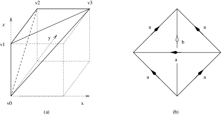
From above we have $\chi(\exp_{3}\!{S^{1}})=1-2+2-1=0$; a well known but still magical fact (see [14, p. 122]) then guarantees that the space formed by gluing the faces of the $3$–simplex in this fashion is a $3$–manifold. Calculating $\pi_{1}(\exp_{3}\!{S^{1}})$ using figure 3(b) we obtain the presentation $\langle a,b|a,a^{2}b^{-1}\rangle$, so $\exp_{3}\!{S^{1}}$ is in fact a simply connected $3$–manifold—and hence almost certainly $S^{3}$, especially given its simple construction. Bott [3] completes the proof by showing it has a genus one Heegaard splitting and appealing to the classification of lens spaces. A more informative approach is the proof of Theorem 3 given below. In appendix A (beginning page A) we will also show directly that $\exp_{3}\!{S^{1}}$ is a $3$–sphere (and that $\exp_{1}\!{S^{1}}$ inside it is a trefoil) using the genus two Heegaard splitting obtained from the triangulation above.

Before proving Theorem 3 a word is necessary on orientation. Given an orientation of $S^{1}$ and a set $\Lambda=\{\lambda,\mu,\nu\}$ of three distinct points in $S^{1}$ we may canonically orient

by positively orienting each of the summands and requiring that the cyclic ordering of $\lambda$, $\mu$, and $\nu$ agree with the orientation of $S^{1}$. This extends to an orientation of $\exp_{3}\!{S^{1}}$ and we regard this as the canonical orientation of $\exp_{3}\!{S^{1}}$. Note that the standard orientation of the simplex $0\leq x\leq y\leq z\leq 1$ of figure 3 co-incides with the canonical orientation of $\exp_{3}\!{S^{1}}$.

To orient $S^{3}$ we regard it as the boundary of the $4$–ball in $\mathbf{C}^{2}$ with its canonical orientation and use the “outward first” convention for induced orientations on boundaries.

Finally we turn our attention to the general case. Proceeding analogously to the two and three dimensional cases we may reduce to the $k$–simplex $0\leq x_{1}\leq\ldots\leq x_{k}\leq 1$. Working somewhat more formally than above let

for $i=0,\ldots,k$, and let $\sigma_{k}$ be the map of the simplex $[v_{0},\ldots,v_{k}]$ to $\exp_{k}\!{S^{1}}$, $\tau_{k-1}$ that of the simplex $[v_{1},\ldots,v_{k}]$. Being a little sloppy with notation we claim:

The lemma enables us to calculate the homology of $\exp_{k}\!{S^{1}}$, obtaining the following.

Theorem 4 for $k\geq 3$ now follows from Corollary 1 and the simple connectivity of $\exp_{3}\!{S^{1}}$ by an application of a standard argument.

We close this section with some remarks on two related spaces. Let

the subsets of $S^{1}$ of size $k$ or less that contain $1$. This subspace has a cell structure with one cell $\tau_{i}$ in each dimension less than or equal to $k-1$, and by (2) the boundary maps are alternately zero and isomorphisms. Thus the reduced homology of $\exp_{k}\!{(S^{1},1)}$ is given by

and moreover $\exp_{k}\!{(S^{1},1)}$ is simply connected for $k\geq 3$ since its 2-skeleton is a dunce cap. It follows (by the Whitehead theorem for $k$ odd, and the argument of Corollary 2 for $k$ even) that $\exp_{k}\!{(S^{1},1)}$ is contractible if $k$ is odd, and homotopy equivalent to $S^{k-1}$ if $k$ is even. The natural map

takes $[\sigma_{k-1}]$ to $[\tau_{k-1}]$ and so is a homotopy equivalence for $k$ even. Note however that this map is not a homeomorphism except when $k=2$ since otherwise $\{\lambda\}$ and $\{\lambda,1\}$ have the same image.

Lastly let

topologised as the direct limit of the $\exp_{k}\!{S^{1}}$, or equivalently, with the CW topology coming from the cell structure consisting of the $\sigma_{i},\tau_{i}$. The full finite subset space $\exp\!{\,S^{1}}$ has vanishing reduced homology in all dimensions and is therefore contractible.

The strategy for proving Theorem 6 is to show that $\exp_{k}\!{S^{1}}\setminus\exp_{k-2}\!{S^{1}}$ deformation retracts to a subspace having the cell structure shown in figure 4. In order to make calculations easier and the result more transparent we will adopt a slightly different picture of $\exp_{k}\!{S^{1}}$, using the action of $S^{1}$ to model it as a quotient of a $(k-1)$–simplex cross an interval. On the simplex level this action corresponds to the constant vector field equal to $(1,1,\ldots,1)$ everywhere and the orbits are unions of intervals of the form

where $y_{i}=x_{i}+1-x_{k}$ for each $i$. The effect of our new model will be to normalise the lengths of these intervals to one. Figure 5 depicts this in the case $k=2$.

Let $\Delta$ be the simplex

and consider the map from $\Delta\times I$ to our usual model

given by

This has inverse

well defined off the codimension two face $[v_{1},\ldots,v_{k-1}]$, which has preimage the entire codimension one face $[v_{1},\ldots,v_{k-1}]\times I$ due to the intervals (3) through these points being stretched from length zero to one. We will refer to this as the “fake face” of $\Delta\times I$ and denote the quotient map $\Delta\times I\rightarrow X\rightarrow\exp_{k}\!{S^{1}}$ by $q$.

In forming $\exp_{k}\!{S^{1}}$ from $\Delta\times I$ the $k-1$ faces $\{a_{1}=0\}\times I$ and $\{a_{i}=a_{i+1}\}\times I$, $1\leq i\leq k-2$, are all identified according to the maps

given by the product of the canonical map with the identity. The face $\{a_{k-1}=1\}\times I$ is collapsed back down to $\{a_{k-1}=1\}$ by projection on the first factor, and $\Delta\times\{0\}$ is glued to $\Delta\times\{1\}$ according to $(a,1)\sim(\phi(a),0)$, where

$\phi$ is affine and permutes the vertices $v_{0},\ldots,v_{k-1}$ cyclicly according to the permutation $i\mapsto i-1\pmod{k-1}$ and so is the canonical map $[v_{0},\ldots,v_{k-1}]\rightarrow[v_{k-1},v_{0},\ldots,v_{k-2}]$. In particular $\exp_{k}\!{S^{1}}\setminus\exp_{k-1}\!{S^{1}}$, as the quotient of $(\mathrm{int}\,\Delta)\times I$, is the mapping torus of $\phi|_{\mathrm{int}\,\Delta}$ and has the homeomorphism type of an $\mathbf{R}^{k-1}$ bundle over $S^{1}$, with monodromy of order $k$. $\phi$ reverses orientation exactly when $k$ is even so the bundle is trivial for $k$ odd and nontrivial for $k$ even.

References

- [1] K Borsuk, On the third symmetric potency of the circumference, Fund. Math. 36 (1949) 236–244
- [2] K Borsuk, S Ulam, On symmetric products of topological spaces, Bull. Amer. Math. Soc. 37 (1931) 875–882
- [3] R Bott, On the third symmetric potency of , Fund. Math. 39 (1952) 264–268
- [4] W Fulton, R MacPherson, A compactification of configuration spaces, Annals of Math. 139 (1994) 183–225
- [5] D Handel, On the configuration spaces of non-empty subsets of the circle of bounded finite cardinality, unpublished work
- [6] D Handel, Some homotopy properties of spaces of finite subsets of topological spaces, Houston J. of Math. 26 (2000) 747–764
- [7] A Hatcher, Notes on basic –manifold topology, in preparation, available on the web at http://www.math.cornell.edu/~hatcher/
- [8] A Hatcher, Algebraic topology, Cambridge University Press (2001), also available on the web at http://www.math.cornell.edu/~hatcher/
- [9] A Illanes, Multicoherence of symmetric products, An. Inst. Mat. Univ. Nac. Autónoma México 25 (1985) 11–24
- [10] N Levitt, Spaces of arcs and configuration spaces of manifolds, Topology 34 (1995) 217–230
- [11] S Macías, On symmetric products of continua, Topology and its Applications 92 (1999) 173–182
- [12] J Milnor, Introduction to Algebraic K-Theory, Princeton University Press (1971)
- [13] J Mostovoy, Lattices in and finite subsets of a circle, preprint (1999) arXiv:math.GT/9911224
- [14] W Thurston, Three-Dimensional Geometry and Topology, volume 1, Princeton University Press (1997)
- [15] A P Ulyanov, Polydiagonal compactification of configuration spaces, J. Algebraic Geom. 11 (2002) 129–159
- [16] M Yoshida, The democratic compactification of configuration spaces of point sets on the real projective line, Kyushu J. Math. 50 (1996) 493–512
Received:\qua22 October 2002