Grope cobordism and Feynman diagramsThanks: The first author was partially supported by NSF VIGRE grant DMS-9983660. The second author was partially supported by NSF grant DMS-0072775 and the Max-Planck Gesellschaft.

James Conant Address: Department of Mathematics
Cornell University
Ithaca, NY 14853-4201 Email address: jconant@math.cornell.edu and Peter Teichner Address: Department of Mathematics, University of California in San Diego, 9500 Gilman Dr, La Jolla, CA 92093-0112 Email address: teichner@euclid.ucsd.edu

Abstract.

We explain how the usual algebras of Feynman diagrams behave under the grope degree introduced in [CT]. We show that the Kontsevich integral rationally classifies grope cobordisms of knots in 3-space when the “class” is used to organize gropes. This implies that the grope cobordism equivalence relations are highly nontrivial in dimension $3$ . We also show that the class is not a useful organizing complexity in $4$ dimensions since only the Arf invariant survives. In contrast, measuring gropes according to “height” does lead to very interesting $4$ -dimensional information [COT]. Finally, several low degree calculations are explained, in particular we show that S-equivalence is the same relation as grope cobordism based on the smallest tree with an internal vertex.

Key words and phrases:

grope cobordism, Feynman diagrams, Vassiliev invariants

1991 Mathematics Subject Classification

57M27

1. Introduction

In [CT] we introduced the notion of a grope cobordism between two knots in 3-space, which places Vassiliev theory in a natural topological context. Gropes are certain 2-complexes built out of several surface stages, whose complexity can be measured by either the class (corresponding to nilpotent groups) or the height (corresponding to solvable groups). The analogy to group theory arises by observing that a continuous map $\phi$ of a circle (into some target space) represents a commutator in the fundamental group if and only if it extends to a map of a surface (which is the simplest possible grope, of class 2 and height 1). Similarly, $\phi$ represents an element in the $k$ -th term of the lower central series (respectively derived series) of the fundamental group if and only if it extends to a continuous map of a grope of class $k$ (respectively height $k$ ).

In knot theory, one replaces continuous maps of a circle by smooth embeddings of a circle into 3-space. Accordingly, one should study embeddings of gropes into 3-space. More precisely, one obtains two sequences of new geometric equivalence relations on the set of knot types by calling two knots equivalent if they cobound an embedded grope (of a specified class or height).

It is the purpose of this paper to show that the invariants associated to grope cobordism are extremely interesting. Let $\mathcal{K}$ be the abelian monoid of knot types, i. e. isotopy classes of oriented knots in 3-space (under connected sum). We proved in [CT] that the quotients $\mathcal{K}/G_{k}:=$ $\mathcal{K}$ modulo grope cobordism of class $k$ in 3-space, are in fact a finitely generated abelian groups. In Section 3.1 we start the investigation of these groups by showing that there is an epimorphism

\mathcal{B}^{g}_{<k}\twoheadrightarrow\mathcal{K}/G_{k},

where $\mathcal{B}^{g}_{<k}$ is the usual (primitive) diagram space known from the theory of finite type invariants but graded by the grope degree. More precisely, $\mathcal{B}^{g}_{<k}$ is the abelian group generated by connected uni-trivalent graphs of grope degree $i,\hskip 11.74988pt1<i<k$ , with at least one univalent vertex and a cyclic ordering at each trivalent vertex. The relations are the usual IHX and AS relations. The grope degree is the Vassiliev degree (i.e. half the number of vertices) plus the first Betti number of the graph. Observe that both relations preserve this new degree.

We then show in Section 3.1 that as in the usual theory of finite type invariants, the above map has an inverse, the Kontsevich integral, after tensoring with the rational numbers. See Definition 3.4 for the definition of the Kontsevich integral $Z^{g}_{<k}$ :

Theorem 1.1.

$Z^{g}_{<k}$ induces an isomorphism of $\mathbb{Q}$ -vector spaces

\mathcal{K}/G_{k}\otimes\mathbb{Q}\cong\mathcal{B}^{g}_{<k}\otimes\mathbb{Q}

This result was inspired by the recent discovery of Garoufalidis and Rozansky [GR] that the Kontsevich integral not only preserves the Vassiliev filtration but also the “loop filtration”, where one grades diagrams by the first Betti number (and correspondingly the clasper surgeries are reorganized). We decided to give an independent proof of Theorem 1.1, by using properties of the Kontsevich integral explained in [Aa] as well as a result from [CT] which says that grope cobordisms can be refined into simple clasper surgeries. In Conjecture 4.5, we take a guess at what the groups $\mathcal{K}/G_{k}$ could be integrally. There is an analogue of this Theorem 1.1 which says that capped grope cobordism is rationally computed by $\mathcal{B}^{v}_{<k}$ , which is the same diagram space as above but graded by the Vassiliev degree. This latter result follows by using work of Habiro, and was announced in [H2].

If one uses class as an organizational tool for grope concordance, i.e. for gropes embedded in $S^{3}\times[0,1]$ and with boundary in $S^{3}\times\{0,1\}$ , then the theory collapses:

Proposition 3.8 .

For each $k\geq 3$ , two knots $K_{i}\subset S^{3}\times\{i\}$ , are class $k$ grope concordant if and only if their Arf invariants agree.

It should be mentioned that Schneiderman has independently given a beautiful geometric argument for the above fact: He directly constructs a weak Whitney tower of class $k$ in 4-space, cobounding two knots with equal Arf invariants. One can then turn this weak Whitney tower into a grope concordance of class $k$ .

It turns out that in order to derive interesting information about knot concordance (i.e. $4$ -dimensional knot theory), one needs to imitate the derived series of a group geometrically. This can be done by restricting attention to gropes which grow symmetrically from the root. Such gropes have a height $h$ and the class $k$ can be calculated as $k=2^{h}$ , exactly as for group commutators. It was shown by Cochran, Orr and Teichner in [COT] that symmetric grope concordance filters the knot concordance group in such a way as to yield all known concordance invariants in the first few steps, leaving a huge tower of concordance invariants yet to be discovered. The first new graded quotient (above the one leading to Casson-Gordon invariants) was shown to be nontrivial in [COT] by using certain von Neumann signatures associated to solvable quotients of the knot group. It is now known [CoT] that all the graded quotients are nontrivial.

Challenge .

Try to understand the equivalence relation of symmetric grope cobordism in 3-space. In particular, determine the role of the von Neumann signatures.

We will show that very interesting things happen even at very small heights. At height $h=1.5$ one gets isomorphism of Blanchfield forms (i.e. S-equivalence) for grope cobordisms in 3-space, whereas the $4$ -dimensional analogue gives cobordism of Blanchfield forms. So in this setting the “kernel” from dimensions $3$ to $4$ is given by connected sums $K\#K^{!}$ , where $K$ is any oriented knot and $K^{!}$ is its reversed mirror image, the concordance inverse.

The reader might be irritated about the occurrence of the non-integral height $h=1.5$ but that’s just a special case of the following equivalence relations on knots: Fix a rooted tree type $\mathcal{T}$ and consider only grope cobordisms of type $\mathcal{T}$ . The notation $\mathcal{T}$ (respectively $c\mathcal{T}$ ) in the following table refers to the equivalence relation given by grope cobordisms (respectively capped grope cobordism) in $3$ -space using gropes of tree-type $\mathcal{T}$ , as explained in [CT]. One can also study grope cobordism in $S^{3}\times[0,1]$ which is denoted by $\mathcal{T}^{4}$ below. Note that in dimension $4$ there is no difference between capped and uncapped grope cobordism because intersections and self-intersections of the caps can always be pushed down into the bottom stage. The following table summarizes our calculations in Section 4.

Theorem 1.2.

For the smallest rooted tree types $\mathcal{T}$ , the grope cobordism (respectively grope concordance) relations are given by the following table:

$\mathcal{K}/c\mathcal{T}$	$\mathcal{K}/\mathcal{T}$	$\mathcal{K}/\mathcal{T}^{4}$
$\{0\}$	$\{0\}$	$\{0\}$
$\mathbb{Z}(c_{2})$	$\mathbb{Z}/2(\text{Arf})$	$\mathbb{Z}/2(\text{Arf})$
$\mathbb{Z}(c_{3})\oplus\mathbb{Z}(c_{2})$	$\mathbb{Z}(c_{2})$	$\mathbb{Z}/2(\text{Arf})$
$\mathbb{Z}(c_{3})\oplus\mathbb{Z}(c_{2})$	$\mathbb{Z}(c_{2})$	$\mathbb{Z}/2(\text{Arf})$
$\begin{array}[]{c}\mathbb{Z}(c_{4})\oplus\mathbb{Z}(c_{4}^{\prime})\oplus\\ \mathbb{Z}(c_{3})\oplus\mathbb{Z}(c_{2})\end{array}$	$\mathbb{Z}/2(c_{3})\oplus\mathbb{Z}(c_{2})$	$\mathbb{Z}/2(\text{Arf})$
$\begin{array}[]{c}\mathbb{Z}(c_{4})\oplus\mathbb{Z}(c_{4}^{\prime})\oplus\\ \mathbb{Z}(c_{3})\oplus\mathbb{Z}(c_{2})\end{array}$	$\mathbb{Z}/2(c_{3})\oplus\mathbb{Z}(c_{2})$	$\mathbb{Z}/2(\text{Arf})$
?	$\begin{array}[]{c}\text{$S$-equivalence}\\ \text{or Bl-forms}\end{array}$	$\begin{array}[]{c}\text{cobordism of}\\ \text{Bl-forms}\end{array}$

Here the $c_{i}$ are generating degree $i$ Vassiliev invariants, and $Bl$ is the Blanchfield form.

Corollary 1.3.

$c_{3}$ modulo two is an S-equivalence invariant.

Challenge .

Understand the monoids $\mathcal{K}/\mathcal{T}$ for more tree types $\mathcal{T}$ .

Our paper ends with Section 5 where we have collected several results that are relevant in the context of grope cobordism. Recall that if a knot $K$ cobounds a grope with the unknot $U$ , then $K$ and $U$ might very well be linked in a nontrivial way. Thus it is a much stronger condition on $K$ to assume that it is the boundary of a grope. For example, if $K$ bounds a grope of class $3$ in $S^{3}$ then the Alexander polynomial vanishes. The following statement generalizes this vanishing result by using the “null-filtration” of [GR], explained in Section 5.1.

Proposition 5.2 .

If a knot $K$ bounds an embedded grope of class $k$ in a $3$ -manifold $M$ , then the pair $(M,K)$ is $(k-3)$ -null equivalent to $(M,U)$ .

The converse is not true for $k=3$ : In $M=S^{3}$ , knots which are null equivalent to the unknot ( $k=3$ above), are exactly knots with trivial Alexander polynomial. On the other hand, knots which bound a grope of class $3$ in $S^{3}$ have a Seifert surface such that the rank of the Seifert form equals the genus of the surface. It is shown in [GT] that this minimal Seifert rank condition is much stronger than having trivial Alexander polynomial.

We invesitgate the behavior of orientation reversal:

Proposition 5.3 .

Let $\rho$ be the map reversing a knot’s orientation. Then for every knot $K$ in the $k$ -th term $G_{k}$ of the grope filtration of $\mathcal{K}$ , one has

K\equiv(-1)^{k}\rho(K)\mod G_{k+1}.

Our final result implies that the main theorem of [CT] can now be phrased as follows: Grope cobordisms of class $k$ in $S^{3}$ are in 1-1 correspondence with sequences of simple clasper surgeries of grope degree exactly $k$ . In [CT] we had to allow simple clasper surgeries of grope degree $\geq k$ .

Theorem 5.4 .

A simple clasper surgery of grope degree $(k+1)$ may be realized by a sequence of simple clasper surgeries of grope degree $k$ .

Acknowledgments: It is a pleasure to thank Stavros Garoufalidis and Kazuo Habiro for useful discussions.

2. Gropes, claspers and diagrams

2.1. Basic notions

For the reader’s convenience we recall some basic notions and results from [CT]. Given a knot $K$ and a disjoint rooted clasper $C$ in a $3$ -manifold $M$ , one can construct a grope cobordism $G(K,C)$ between $K$ and $K_{C}$ in $M$ , where $K_{C}$ is the surgery of $K$ along $C$ . The “root” of the clasper is a simple leaf (i.e. a leaf with an embedded cap intersecting $K$ once) which makes sure that the ambient $3$ -manifold $M$ is unchanged. Caps of a clasper $C$ are disjointly embedded disks with interiors disjoint from $C$ , which bound some of the leaves of $C$ . The grope cobordism $G(K,C)$ is capped if all the leaves of the clasper have caps, which are allowed to intersect the knot. (If there is a single cap disjoint from $K$ then $K_{C}$ is isotopic to $K$ .) Finally, in a simple clasper, all the leaves have caps and the knot intersects each cap exactly once. Thus this notion only makes sense for the pair $(K,C)$ .

The class of $G(K,C)$ is given by the grope degree of the clasper. Recall that a clasper $C$ has an underlying uni-trivalent graph $\Gamma$ which is obtained by removing the leaves and collapsing to the spine. The grope degree of $C$ is defined as the Vassiliev degree plus the first Betti number of $\Gamma$ . The Vassiliev degree is one half the number of vertices of $\Gamma$ .

The construction of $G(K,C)$ depends on a choice of $b_{1}(\Gamma)$ many “cuts”, which turn $\Gamma$ into a rooted tree, giving the precise grope type of $G(K,C)$ . Note that each cut increases the Vassiliev degree by one, but leaves the grope degree unchanged, as it should. Note also that a cut introduces a pair of Hopf-linked leaves into the clasper, and hence the resulting grope cobordism cannot have two disjoint caps at the corresponding tips. This explains why capped grope cobordism corresponds to the Vassiliev degree: cuts are not allowed (since caps must be disjointly embedded), and for trees the two degrees agree.

Let $\mathcal{K}$ denote the monoid of oriented knot types in 3-space (with respect to connected sum), and let $\mathcal{K}/G_{k}$ be $\mathcal{K}$ modulo the equivalence relation of grope cobordism of class $k$ . It turns out that this is an abelian group. By Theorem 2 of [CT], a grope cobordism of class $k$ corresponds to a sequence of simple clasper surgeries of grope degree $\geq k$ . We will show in Theorem 5.4 that a grope cobordism of class $k$ also corresponds to a sequence of simple clasper surgeries of grope degree exactly equal to $k$ .

Let $\mathcal{K}/G^{c}_{k}$ denote the abelian group of oriented knot types modulo capped grope cobordism of class $k$ in 3-space. Capped grope cobordism of class $k$ coincides with Vassiliev degree $k$ simple clasper surgeries, and with Vassiliev $(k-1)$ -equivalence. By letting $G_{k}$ be the subset of knots which are class $k$ grope cobordant to the unknot (and similarly $G^{c}_{k}$ for capped grope cobordisms) we can form the associated graded quotients

\mathcal{G}_{k}:=G_{k}/G_{k+1}\hskip 11.74988pt\text{ respectively }\hskip 11.74988pt\mathcal{G}^{c}_{k}:=G^{c}_{k}/G^{c}_{k+1}

These graded quotients will be related in Lemmas 2.1 and 3.2 to certain Feynman diagrams of a fixed degree.

Let $\mathcal{T}$ be a rooted tree type. Then $\mathcal{K}/\mathcal{T}$ is defined as the monoid of knots modulo $\mathcal{T}$ grope cobordism. Define $\mathcal{K}/\mathcal{T}^{c}$ to be the monoid of knots modulo capped $\mathcal{T}$ grope cobordism. A capped $\mathcal{T}$ grope cobordism corresponds to a sequence of simple tree clasper surgeries of type $\mathcal{T}$ . As a consequence, $\mathcal{K}/\mathcal{T}^{c}$ depends only on the unrooted tree type.

2.2. Feynman diagrams

Let $\widetilde{\mathcal{A}}_{k}$ denote the free abelian group generated by connected trivalent graphs with $2k$ vertices and one distinguished (oriented) cycle, such that each trivalent vertex has a cyclic orientation.¹¹ 1 Since trivalent vertices that lie on the distinguished cycle can be canonically oriented, the convention in much of the literature is to not orient these vertices. The distinguished cycle is often called “the outer circle,” and the rest is sometimes called “the dashed part.”

Define $\mathcal{A}_{k}$ to be the quotient of $\widetilde{\mathcal{A}}_{k}$ by the usual IHX and AS relations. The AS (antisymmetry) relation is a relation of the form $G_{1}+G_{2}=0$ , where the $G_{i}$ differ by a cyclic orientation at a given vertex. The IHX relation is pictured in Figure 1. If the distinguished cycle runs through the part of the diagram involved in an IHX relation, the relation is called an STU relation. As proven in [BN], STU relations generate all IHX relations.

Refer to caption — Figure 1. The IHX relation.

Then $\mathcal{A}=\oplus_{k}\mathcal{A}_{k}$ is the well-known algebra of Feynman diagrams. (Feynman diagrams enjoy a plethora of other names, but we will stick to this one.) The algebra structure is given by “connected sum”, which turns out to be well-defined. Moreover, $\mathcal{A}$ is a graded Hopf algebra as explained in [BN]. The primitive elements $\operatorname{Prim}(\mathcal{A})$ are generated by diagrams which stay connected when removing the outer circle. However, such diagrams are not closed under the STU relation, so it is convenient to also consider the group $\mathcal{A}^{I}:=\mathcal{A}_{>0}/\mathcal{A}_{>0}^{2}$ of indecomposable elements. Since $\mathcal{A}$ is a commutative and cocommutative Hopf algebra, a famous theorem of Milnor and Moore implies that, say over $\mathbb{Q}$ , $\mathcal{A}$ is a polynomial algebra in the primitive elements. In particular,

\operatorname{Prim}(\mathcal{A})\otimes\mathbb{Q}\cong\mathcal{A}^{I}\otimes\mathbb{Q}.

There is an analogous abelian group of diagrams $\mathcal{B}$ defined just like $\mathcal{A}$ but without an outer circle. Here the subspace of connected diagrams is closed under IHX and AS relations, so that the above problem for primitives does not occur. There is an averaging map $\chi:\mathcal{B}\to\mathcal{A}$ which puts back the outer circle in all possible ways. It was shown in [BN] that this is rationally an isomorphism.

Since we will only be interested in connected diagrams, we define $\mathcal{B}^{v}_{k}$ to be the abelian group spanned by connected uni-trivalent graphs with $2k$ vertices (such that each trivalent vertex has a cyclic orientation, and with at least one univalent vertex) modulo the AS and IHX relations. Since we are dealing with unframed knots, we just set the groups $\mathcal{B}^{v}_{k}:=0$ for $k=0,1$ . Define the graded abelian group

\mathcal{B}^{v}:=\oplus_{k}\mathcal{B}^{v}_{k}.

The superscript ‘ $v$ ’ indicates that we are using the Vassiliev degree, and it also serves to distinguish from the usual group $\mathcal{B}$ (which would also contain non-connected diagrams). As a consequence of these definitions, one has an averaging isomorphism of graded vector spaces

(1)

\chi:\mathcal{B}^{v}\otimes\mathbb{Q}\overset{\cong}{\longrightarrow}\mathcal{A}^{I}\otimes\mathbb{Q}.

We shall show that these groups, modulo terms of degree $>k$ , are isomorphic to $\mathcal{K}/G^{c}_{k}\otimes\mathbb{Q}$ .

2.3. Maps relating capped gropes and Feynman diagrams

There is a well-known map that sends a chord diagram to an alternating sum over crossing changes on the unknot guided by the chords. This map can in fact be extended to all diagrams, as in the next lemma, whose proof is found in the next section.

Lemma 2.1.

For each $k>1$ , there is an epimorphism

\Phi_{k}:\mathcal{A}^{I}_{k}\longrightarrow\mathcal{G}^{c}_{k}.

defined by sending a diagram to the alternating sum over clasper surgeries corresponding to each connected component of “the dashed part.”

The (unframed) Kontsevich integral is a map on isotopy classes of oriented knots

Z:\mathcal{K}\longrightarrow\widehat{\mathcal{A}}:=\prod_{k}\mathcal{A}_{k}\otimes\mathbb{Q}

which sends connected sums of two knots to their product in $\widehat{\mathcal{A}}$ . The image of $Z$ lies inside the group-like elements of the complete Hopf algebra $\widehat{\mathcal{A}}$ . Thus we may compose it with the logarithm in this complete Hopf algebra to end up in the subspace of primitive elements. Then $\log Z$ takes connected sum to addition! Now decompose $\log Z$ according to Vassiliev degree and denote the degree $k$ part by

Z_{k}^{v}:\mathcal{K}\longrightarrow\operatorname{Prim}(\mathcal{A}_{k})\otimes\mathbb{Q}\cong\mathcal{A}^{I}_{k}\otimes\mathbb{Q}.

Then $Z_{k}^{v}$ factors through simple clasper surgeries of degree $k+1$ by [H2], and hence through $\mathcal{K}/G^{c}_{k+1}$ by [CT]. Restricting to knots in $G^{c}_{k}$ we get a homomorphism

Z_{k}^{v}:\mathcal{G}^{c}_{k}\longrightarrow\mathcal{A}^{I}_{k}\otimes\mathbb{Q}.

The definition of $\Phi_{k}$ given in the next section, and in particular the fact that it extends the original definition on chord diagrams, implies by the universality of the Kontsevich integral the following

Lemma 2.2.

$Z_{k}^{v}\circ\Phi_{k}=Id$ .

This shows that $\Phi_{k}$ is an isomorphism modulo torsion because $\mathcal{A}_{k}$ are finitely generated.

2.4. Clasper forests and Feynman diagrams

It is the goal of this section to show that the map $\Phi_{k}$ extends to all diagrams in a natural way. This will lead to Lemma 2.13 which will be used in the proof of Theorem 4.2. This material is well-known to the experts and was essentially announced by Habiro in [H2]. A complication we face is that we include all capped claspers, not just those which are trees. Since Habiro usually restricts to trees, we need to include some extra arguments for the general case.

We begin with some definitions which will be used in this section.

Definitions 2.3.

•

A CC-set is a union of finitely many disjoint capped claspers on a knot $K$ .
•

The degree of a CC-set is the minimum of the degrees of each connected component.
•

A CC-scheme is a collection $\{\mathcal{C}_{1},\mathcal{C}_{2},\ldots,\mathcal{C}_{l}\}$ where each $\mathcal{C}_{i}$ is a CC-set .
•

The degree of a CC-scheme is the sum of the degrees of each $\mathcal{C}_{i}$ .
•

A CC-scheme is called simple if each CC-set is a single simple clasper.
•

Let $\mathcal{S}=\{\mathcal{C}_{1},\mathcal{C}_{2},\ldots,\mathcal{C}_{l}\}$ be a CC-scheme on a knot $K$ . Define $[K;\mathcal{S}]=\sum_{\sigma\subset\mathcal{S}}(-1)^{l+|\sigma|}K_{\sigma}\in\mathbb{Z}[\mathcal{K}],$ where $K_{\sigma}$ is the knot modified by each CC-set in $\sigma$ .

We list a couple of useful facts about brackets.

Lemma 2.4.

Let $\mathcal{C}_{1},\mathcal{C}_{2}$ be disjoint CC-sets on $K$ and denote by $\mathcal{C}_{1}\cup\mathcal{C}_{2}$ the CC-set which is the union of $\mathcal{C}_{1}$ and $\mathcal{C}_{2}$ . If $\mathcal{S}$ is a CC-scheme on $K$ , disjoint from $\mathcal{C}_{1}\cup\mathcal{C}_{2}$ , then

[K;\{\mathcal{C}_{1}\cup\mathcal{C}_{2}\}\cup\mathcal{S}]=[K;\{\mathcal{C}_{1}\}\cup\mathcal{S}]+[K_{\mathcal{C}_{1}};\{\mathcal{C}_{2}\}\cup\mathcal{S}],

See [G], Lemma 5.2 mutatis mutandis.

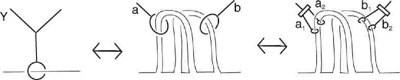
Lemma 2.5.

Consider the central part of Figure 2, with two disjoint capped claspers $a,b$ , disjoint from a CC-scheme $\mathcal{S}$ . Then

[K;\{a\}\cup\{b\}\cup\mathcal{S}]=[K;\{a\cup b\}\cup\mathcal{S}]

Proof.

If $\sigma\subset\mathcal{S}$ then $K_{\{a\}\cup\sigma}=K_{\sigma}=K_{\{b\}\cup\sigma}$ . This implies $[K_{a};\mathcal{S}]=[K_{b};\mathcal{S}]=[K;\mathcal{S}]$ and hence

	$\displaystyle[K;\{a\}\cup\{b\}\cup\mathcal{S}]$	$\displaystyle=[K;\mathcal{S}]-[K_{b};\mathcal{S}]-[K_{a};\mathcal{S}]+[K_{a\cup b};\mathcal{S}]$
		$\displaystyle=-[K;\mathcal{S}]+[K_{a\cup b};\mathcal{S}]$
		$\displaystyle=[K;\{a\cup b\}\cup\mathcal{S}]$

∎

The linear span of all knot types, $\mathbb{Z}[\mathcal{K}]$ , can be filtered by defining $\mathcal{F}^{v}_{k}\subset\mathbb{Z}[\mathcal{K}]$ to be the linear span of all brackets $[K;\mathcal{S}]$ where $\mathcal{S}$ is of degree $k$ .

Lemma 2.6.

If $C$ is a clasper on a knot disjoint from a CC-scheme $\mathcal{S}$ , then $[K;\mathcal{S}]-[K_{C};\mathcal{S}]\in\mathcal{F}^{v}_{|\mathcal{S}|+|C|}$ .

Proof.

This is just the simple calculation $[K;\mathcal{S}\cup\{C\}]=[K;\mathcal{S}]-[K_{C};\mathcal{S}]$ . ∎

The following proposition explains the superscript “ $v$ .”

Proposition 2.7.

$\mathcal{F}^{v}_{k}\subset\mathbb{Z}[\mathcal{K}]$ agrees with the usual Vassiliev filtration of $\mathbb{Z}[\mathcal{K}]$ .

Proof.

One can take the usual Vassiliev filtration to be defined by brackets where each CC-set is a single simple degree $1$ clasper. Thus $\mathcal{F}^{v}_{k}$ contains the usual Vassiliev filtration.

The converse follow from Theorem 6.7 (3) of [H2], with one complication. Namely, that Theorem is phrased only for tree claspers, but it can be easily enhanced to work for all capped claspers. The proof works by applying the move from Lemma 2.5, thereby breaking a clasper into two claspers of lower degree. Iterating, one reduces all of the trees to degree one capped claspers. This fails for graphs if in Figure 2, the two claspers $a$ and $b$ are the same clasper. In this case we’ve still made progress since there are a reduced number of loops. To be precise, induct on the number of internal vertices. (Compare the proof of Lemma 2.8.) ∎

Lemma 2.8.

On a knot $K$ , let $\mathcal{S}_{1}=\{C^{1}_{1},\ldots,C_{l}^{1}\}$ and $\mathcal{S}_{2}=\{C^{2}_{1},\ldots,C^{2}_{l}\}$ be two CC-schemes of degree $k$ , where each CC-set consists of a single clasper. Suppose the CC-schemes differ only by a homotopy of an edge of one of the claspers. Then

[K;\mathcal{S}_{1}]-[K;\mathcal{S}_{2}]\in\mathcal{F}^{v}_{k+1}.

Proof.

A homotopy of an edge can be realized by a degree one clasper, one leaf of which links the edge and the other leaf being embedded arbitrarily away from the caps. Using the zip construction, this can be realized by degree one claspers $E$ where one leaf links the edge, and the other leaf either: is a meridian to an edge, is a meridian to the knot, or is a trivial 1-framed leaf. This last case is covered by Corollary 2.11. We prove the other two cases by induction on the number of trivalent vertices. The base case is when all the claspers $C^{i}_{j}$ are of degree one (eyeglasses). Then the leaves of the clasper $E$ can be slid off the end of the (up to two) eyeglasses that it links, introducing two new intersections with the knot for each one. Let the slid clasper be called $E^{\prime}$ . Then we have argued

[K;\mathcal{S}_{2}]=[K_{E^{\prime}};\mathcal{S}_{1}].

By Lemma 2.6 we are done. Now suppose that a pair $C^{1}_{j},C^{2}_{j}$ has a trivalent vertex. Apply Figure 2 to a leg of $C^{i}_{j}$ , denoting the resulting claspers by $a^{i},b^{i}$ . (If $E$ happens to link the leg we are expanding, push it off so that it links the knot instead.) If $a^{i}$ and $b^{i}$ are different, then Lemma 2.5 implies that, defining $\mathcal{S}^{\prime}_{i}=\{C^{i}_{1},C^{i}_{2},\ldots,C^{i}_{j-1},a^{i},b^{i},C^{i}_{j+1},\ldots,C^{i}_{l}\}$ ,

[K;\mathcal{S}_{i}]=[K;\mathcal{S}^{\prime}_{i}]

and since $\mathcal{S}^{\prime}_{1},\mathcal{S}^{\prime}_{2}$ differ by the homotopy coming from $E$ , $[K;\mathcal{S}^{\prime}_{1}]=[K;\mathcal{S}^{\prime}_{2}]\mod\mathcal{F}^{v}_{k+1}$ by induction. If $a^{i}=b^{i}$ , life is even simpler: define

\mathcal{S}^{\prime\prime}=\{C^{i}_{1},C^{i}_{2},\ldots,C^{i}_{j-1},a^{i},C^{i}_{j+1},\ldots,C^{i}_{l}\}.

Then $[K;\mathcal{S}]=[K;\mathcal{S}^{\prime\prime}]$ and we are done by induction as above. ∎

Lemma 2.9.

Let $C$ be a tree clasper on a knot $K$ . There is a clasper $\widetilde{C}$ in a regular neighborhood of $C$ such that $K_{C\cup\widetilde{C}}=K$ . Moreover, the leaves of $C$ and $\widetilde{C}$ are parallel (in the given framing of $C$ ) and one may arrange the edges of $\widetilde{C}$ which go through a regular neighborhood of a leaf of $C$ to be parallel to the leaves of $C$ .

In Figure 3(a), the above process is depicted in the vicinity of a Hopf-pair of $C$ . (The two degree $1$ claspers labelled $E$ are not relevant now.)

Proof.

The clasper $\widetilde{C}$ is constructed using Figure 27 of [H2] and the version of the zip construction in [CT, Sec.4]. ∎

Lemma 2.10.

Let $C$ and $C^{\prime}$ be two simple claspers of degree $k$ on a knot $K$ , which differ by a single half-twist. Then $K_{C}+K_{C^{\prime}}-2K\in\mathcal{F}^{v}_{k+1}$ .

Proof.

Insert Hopf-pairs of leaves to make $C$ a tree clasper and let $\widetilde{C}$ be an inverse to $C$ , as in Lemma 2.9. For each (non-root) cap of $C$ and $\widetilde{C}$ there is a degree 1 clasper (or eyeglass), surgery on which pushes the knot out of the cap. Choose one of the leaves in each Hopf pair of $C$ . As this can be regarded as an additional cap of the tree clasper, there is an eyeglass which pushes everything out of this leaf, just like above. See Figure 3 for an example of these eyeglasses $E_{i}$ . Let $\mathcal{E}_{1}$ denote the CC-scheme whose elements are the (at least $k$ ) eyeglasses which push things out of $C$ , and let $\mathcal{E}_{2}$ be the same, only for $\widetilde{C}$ . The claspers in $\mathcal{E}=\mathcal{E}_{1}\cup\mathcal{E}_{2}$ are capped, when considered on the knot $K=K_{C\cup\widetilde{C}}$ . Note that $K_{\sigma}=K$ if $\sigma$ has nontrivial intersection with $\mathcal{E}_{1}$ and with $\mathcal{E}_{2}$ . If $\emptyset\neq\sigma\subset\mathcal{E}_{1}$ , then $K_{\sigma}=K_{\widetilde{C}}$ . If $\emptyset\neq\sigma\subset\mathcal{E}_{2}$ then $K_{\sigma}=K_{C}$ . This analysis implies that

-[K;\mathcal{E}]=K_{C}+K_{\widetilde{C}}-2K.

The left-hand side is in $\mathcal{F}^{v}_{2k}\subset\mathcal{F}^{v}_{k+1}$ .

This is almost what we want, except that $\widetilde{C}$ has edges that wind around itself and may wind through the Hopf pairs of leaves. Let $\mathcal{E}_{3}$ be the CC-scheme consisting of $k$ degree $1$ claspers on $K_{\widetilde{C}}$ , which push things out of the leaves. There is an additional clasper, denoted by $E$ which pushes the edges out of the other disk in each Hopf pair. It is a union of eyeglasses, one for each leaf, see Figure 3(b). Now

[K_{\widetilde{C}};\mathcal{E}\cup\{E\}]=K_{\widetilde{C}}-K_{\overline{C}},

where $\overline{C}$ is formed from $\widetilde{C}$ by applying $E$ . Symmetrically we can push the edges out of the other leaves in each Hopf pair, modulo $\mathcal{F}^{v}_{k+1}$ to get the clasper $C^{\prime}$ in the statement of the lemma. ∎

Corollary 2.11.

Let $C_{1}$ and $C_{2}$ be two claspers on a knot $K$ which differ by a full twist along an edge. Then $K_{C_{1}}-K_{C_{2}}\in\mathcal{F}^{v}_{k+1}$ .

Proof.

Let $C$ be a clasper that differs from both $C_{1}$ and from $C_{2}$ by a half-twist. Then Lemma 2.10 implies that $K_{C_{1}}=2K-K_{C}=K_{C_{2}}\mod\mathcal{F}^{v}_{k+1}$ . ∎

Let $\mathcal{CF}_{k}$ be the set of pairs $(K,\mathcal{S})$ where $K\in\mathcal{K}$ and $\mathcal{S}$ is a simple CC-scheme of degree $k$ on the knot $K$ . These are considered up to isotopy. The bracket defines a map $\mathcal{CF}_{k}\to\mathbb{Z}[\mathcal{K}]$ . One can also define a map

\Psi:\mathcal{CF}_{k}\to\mathcal{A}_{k}

as follows: The unoriented trivalent graph, $D$ , associated to $(K,\mathcal{S})$ is gotten by collapsing simple leaves to points and forgetting the embedding. The distinguished cycle is the knot. The orientation of the Feynman diagram is more subtle. Recall that each clasper $C_{i}$ is a certain thickening of a graph. Hence $C_{i}$ may not be orientable (even though the thickened leaves are because they have integral framing, and hence a full number of twists). However, each $C_{i}$ may be made orientable by replacing $l_{i}$ bands by half-twisted bands, where $l_{i}$ is the dimension of the $2$ -torsion subgroup of $H_{1}(C_{i})$ . Do this, and let $l=\sum l_{i}$ be the total number of half twisted bands glued in to every $C_{i}$ . Now choose orientations of each new thickening $C_{i}$ . These give rise to cyclic orders of the in-coming edges at each node. Denote the induced orientation of $D$ by $or$ . The choice of orientation also determines a normal direction. Let $m$ be the number of leaves where the knot pierces contrary to the distinguished normal direction. Now $\Psi(K,\mathcal{S})=(-1)^{m+l}(D,or)$ . $\Psi$ is well defined. It does not depend on the choice of orientations, because the parity of the number of leaves of each $C_{i}$ is the same as the parity of the number of nodes. The key thing to notice about this orientation convention is that it switches under the introduction of a half-twist in any edge of a clasper in $\mathcal{S}$ .

Now we can define the homomorphism

\Phi_{k}:\mathcal{A}^{I}_{k}\to\mathcal{G}^{c}_{k}

from Lemma 2.1 as follows: For an oriented diagram $D\in\widetilde{A}_{k}$ , define $\Phi_{k}(D):=cs_{k}([U;\mathcal{S}])$ , for some framed embedding $\mathcal{S}$ of the diagram $D$ on the unknot $U$ , so that $\Psi(U,\mathcal{S})=D$ . (Note that framed embedded diagrams can be regarded as simple CC-schemes ). Here $cs_{k}:\mathbb{Z}[\mathcal{K}]\to\mathcal{K}/G^{c}_{k+1}$ is the map given by sending addition to connected sum.

By definition, $\Phi_{k}$ vanishes on diagrams of degree $>k$ and, by Proposition 2.7 lands in $\mathcal{G}^{c}_{k}=\mathcal{F}^{v}_{k}/\mathcal{F}^{v}_{k+1}$ . This, together with Lemma 2.8 and Corollary 2.11, implies that, extending linearly, we get a well defined map:

\displaystyle\Phi_{k}\colon\widetilde{A}_{k}\to\mathcal{G}^{c}_{k}

This means that the choice of the framed embedding of the diagram $D$ is irrelevant. Clearly $\Phi_{k}=0$ on separated diagrams, so it will factor through $\mathcal{A}^{I}_{k}$ . Thus to get a map on $\mathcal{A}_{k}$ , we only need to show that $\Phi_{k}$ vanishes on the STU- and AS-relations.

Lemma 2.12.

$\Phi_{k}$ vanishes on all STU and AS relations.

Proof.

First we show it vanishes on AS relations. Suppose $D_{1}$ and $D_{2}$ are two diagrams that differ by a cyclic order at one vertex. Let $C_{1}$ be a clasper representing $D_{1}$ : $\Phi_{k}(D_{1})=U_{C_{1}}$ . Let $C_{2}$ be the same, except for three half-twists on the edges incident to the vertex. By our orientation conventions, $\Phi_{k}(D_{2})=U_{C_{2}}$ . Applying Lemma 2.10 three times, with $K=U$ , we see that

\Phi_{k}(D_{1}+D_{2})=U_{C_{1}}\#U_{C_{2}}=0\hskip 11.74988pt\in\mathcal{G}^{c}_{k},

as desired. Next we consider the STU relation. Let $\widetilde{\Phi}_{k}:\widetilde{A}_{k}\to\mathbb{Z}[\mathcal{K}]$ be the lift of $\Phi_{k}$ discussed above, i. e. before applying the summation maps $cs_{k}$ . Consider an STU relation $D_{s}=D_{t}-D_{u}$ , where $D_{s}$ has one more trivalent vertex than $D_{t}$ and $D_{u}$ . Let Y be the component of the dashed part of $D_{s}$ which has the additional vertex. Then

\displaystyle\widetilde{\Phi}_{k}(D_{s})=[U;\{Y,C_{2},\ldots,C_{l}\}]

where the clasper representing Y is also called Y, and is pictured in Figure 2. The claspers $a$ and $b$ from Figure 2 can be further subdivided into claspers $a_{1},a_{2},b_{1},b_{2}$ using the zip construction, assuming that $a$ and $b$ are not the same clasper. By the previous lemmas we have

			$\displaystyle[U;\{a\cup b,C_{2},\ldots,C_{l}\}]$
		$\displaystyle=$	$\displaystyle[U;\{a,b,C_{2},\ldots,C_{l}\}]$
		$\displaystyle=$	$\displaystyle[U;\{a_{1}\cup a_{2},b_{1}\cup b_{2},C_{2},\ldots,C_{l}\}]$
		$\displaystyle=$	$\displaystyle[U;\{a_{1},b_{1},C_{2},\ldots,C_{l}\}]+[U_{b_{1}};\{a_{1},b_{2},C_{2},\ldots,C_{l}\}]$
			$\displaystyle+[U_{a_{1}};\{a_{2},b_{1},C_{2},\ldots,C_{l}\}]+[U_{a_{1}\cup b_{1}};\{a_{2},b_{2},C_{2},\ldots,C_{l}\}]$
		$\displaystyle\equiv$	$\displaystyle[U;\{a_{1},b_{1},C_{2},\ldots,C_{l}\}]+[U;\{a_{1},b_{2},C_{2},\ldots,C_{l}\}]$
			$\displaystyle+[U;\{a_{2},b_{1},C_{2},\ldots,C_{l}\}]+[U;\{a_{2},b_{2},C_{2},\ldots,C_{l}\}]\mod\mathcal{F}^{v}_{k+1}(\mathbb{Z}\mathcal{K})$
		$\displaystyle=$	$\displaystyle-\widetilde{\Phi}_{k}(D_{t})+\widetilde{\Phi}_{k}(D_{t})-\widetilde{\Phi}_{k}(D_{u})-\widetilde{\Phi}_{k}(D_{t})=\widetilde{\Phi}_{k}(D_{t})-\widetilde{\Phi}_{k}(D_{u})$

If, in Figure 2, the two claspers $a$ and $b$ are really two ends of the same clasper, we use the construction of Proposition 4.6 of [H2] instead. See Figure 4 which is a clasper identity of [H2].

Let $D_{s},D_{t},D_{u}$ be the three diagrams in an STU relation such that the corresponding $a$ and $b$ claspers are part of the same clasper. Then

$\displaystyle\widetilde{\Phi}_{k}(D_{u})$	$\displaystyle=$	$\displaystyle[U;\{\overline{U},C_{2},\ldots,C_{l}\}]=[U;\{\{\overline{T},\overline{S}\},C_{2},\ldots,C_{l}\}]$
	$\displaystyle=$	$\displaystyle[U;\{\overline{T},C_{2},\ldots,C_{l}\}]+[U_{\overline{T}};\{\overline{S},C_{2},\ldots,C_{l}\}]$
	$\displaystyle\equiv$	$\displaystyle[U;\{\overline{T},C_{2},\ldots,C_{l}\}]+[U;\{\overline{S},C_{2},\ldots,C_{l}\}]$
	$\displaystyle=$	$\displaystyle\widetilde{\Phi}_{k}(D_{t})+\widetilde{\Phi}_{k}(D_{s})$

∎

The proof of Lemma 2.1 is now complete.

Lemma 2.13.

Let $C$ be a simple clasper surgery of Vassiliev degree $k$ on a knot $K$ . Let $D$ be the diagram obtained by thinking of the clasper as the dashed part, and of the knot as the outer circle. Then $\Phi_{k}(\pm D)=K_{C}\#K^{-1}\in\mathcal{G}^{c}_{k}.$

Remark 2.14.

Here is a sketch of a proof that Lemma 2.13 is true rationally. The proof that it is true integrally is given below. One can think of the Kontsevich integral of $K_{C}-K$ as the Aarhus integral of the difference of two links $K\cup L_{C}-K$ , where $L_{C}$ is the link associated to the simple clasper. Now, it is not hard to show that the lowest degree term of the Aarhus integral is exactly the diagram corresponding to the graph type of the clasper. (By arguments analogous to those in section 3.3 of [GR]. In the absence of a knot $K$ , this is the statement that the Aarhus/LMO invariant is universal with respect to Goussarov’s Y-filtration.) Now the result follows by Lemma 2.2.

Proof of 2.13.

Let $\widetilde{C}$ be a clasper on the unknot with diagram $D$ . Put in half-twists so that it has the same sign as $C$ . By definition, $\Phi_{k}(D)=U_{\widetilde{C}}=U_{\widetilde{C}}\#K\#K^{-1}$ . By Lemma 2.8, we can move $\widetilde{C}$ into a position corresponding to the clasper $C$ on the knot $K$ . Using Corollary 2.11, we can add an even number of half-twists until the framings agree. ∎

3. The grope degree

We first introduce a second degree on the graphs $\Gamma$ generating $\mathcal{B}^{v}$ :

Definition 3.1.

The grope degree of $\Gamma$ is

g(\Gamma):=b_{1}(\Gamma)+v(\Gamma).

Let $\mathcal{B}^{g}_{k}$ be the grope degree $k$ part of the group $\mathcal{B}^{v}$ .

We note that the grope degree is preserved by the IHX and AS relations, and hence really gives a new graded abelian group

\mathcal{B}^{g}:=\oplus_{k}\mathcal{B}^{g}_{k}.

3.1. Feynman diagrams and the grope degree

In a similar fashion to $\Phi_{k}$ , we define a surjective map

\Phi^{g}_{k}:\mathcal{B}^{g}_{k}\to\mathcal{G}_{k}

on connected Feynman diagrams of grope degree $k$ as follows. For a connected diagram $D\in\widetilde{\mathcal{B}}_{k}$ , let $\widetilde{D}\in\widetilde{A}_{k}$ be a diagram formed by attaching the univalent vertices of $D$ to the outer circle in some order. Let $(U,C)\in\mathcal{C}\mathcal{F}^{v}_{k}$ satisfy $\Psi(U,C)=\widetilde{D}$ , where $C$ is a single clasper of grope degree $k$ , and $U$ is the unknot. Now define

\Phi_{k}^{g}(D):=U_{C}\in\mathcal{K}/G_{k+1}.

In the previous section we used various lemmas of Habiro [H2] (for moving claspers around modulo higher Vassiliev degree) in order to show that $\Phi_{k}$ is well defined. Section 3.3 contains the relevant lemmas in the case of grope degree. In fact, we need to show that $\Phi_{k}^{g}$ does not depend on the order in which we attached the univalent vertices, and that AS and IHX get killed. The independence of order follows from Lemma 3.9(a), and the AS and IHX relations follow from 3.11(a) and 3.11(c). We have thus proven the following analogue of Lemma 2.1.

Lemma 3.2.

For each $k>1$ , there is an epimorphism

\Phi^{g}_{k}:\mathcal{B}^{g}_{k}\longrightarrow\mathcal{G}_{k}

In order to show that $\Phi^{g}_{k}$ is rationally an isomorphism, we want to study the behavior of the Kontsevich integral with respect to the grope degree.

Recall that there is an isomorphism $\hat{\mathcal{A}}\cong\hat{\mathcal{B}}$ of graded algebras given by the composition $\partial_{\Omega}\sigma$ , where $\sigma:\hat{\mathcal{A}}\to\hat{\mathcal{B}}$ is the inverse of the averaging map $\chi$ from equation 1, and $\partial_{\Omega}$ is the “wheeling” automorphism of $\hat{\mathcal{B}}$ [T]. Here $\hat{\mathcal{A}}$ has the multiplication given by connected sum, whereas on $\hat{\mathcal{B}}$ the multiplication is just disjoint union. It follows that

(2)

\log_{\hat{\mathcal{B}}}(\partial_{\Omega}\sigma)=(\partial_{\Omega}\sigma)\log_{\hat{\mathcal{A}}}.

Following [GR], define the Euler degree of a diagram in $\mathcal{B}$ to be the number of internal trivalent vertices, which by definition are trivalent vertices not adjacent to univalent vertices. It is called Euler degree because for uni-trivalent graphs $\Gamma$ one has

e(\Gamma)=2(b_{1}(\Gamma)-b_{0}(\Gamma)).

Decompose the composition $\log_{\hat{\mathcal{B}}}(\partial_{\Omega}\sigma)Z$ according to Euler degree to obtain

Z^{e}_{k}:\mathcal{K}\to\mathcal{B}^{e}_{k}

as the Euler degree $k$ part of the “Kontsevich integral”. The following proposition follows by work of Garoufalidis and Rozansky [GR] using [Aa], but for the sake of completeness we provide an argument using only [Aa].

Proposition 3.3.

Let $C$ be a simple clasper of Euler degree $n$ on a knot $K$ . Then $Z^{e}_{m}(K)-Z_{m}^{e}(K_{C})=0$ for all $m<n$ .

Proof.

We factor through the Aarhus integral, $A$ , of pairs $(M,K)$ , [Aa]. When normalized appropriately, $A(S^{3},K)=\sigma Z(K)$ . (In the definition of the Aarhus integral we apply $\sigma$ to the knot $K$ as well as to the surgery link components.) We will assume familiarity with the Aarhus integral in the following proof.

Break $C$ into a union of $Y$ ’s. If a $Y$ has no leaf that links the knot, it will be called internal since the corresponding trivalent vertex is internal. Each $Y$ has an associated $6$ component link. Let the three components in the Borromean rings be called the “B” components, and the three other components be called the “L” components. Let the link corresponding to the union of all Y’s be called $L_{C}$ . Fix balls which meet the link at the Borromean rings corresponding to internal Y’s as on the left hand side of Figure 5.

For each ball, there is an associated move that replaces the tangle on the left of Figure 5 with the trivial one on the right. Let $S$ be the set of such moves, one for each internal vertex of $C$ . Consider the alternating sum $[K\cup L_{C};S]$ . Then the (alternating sum of) Kontsevich integrals $Z[K\cup L_{C};S]$ can be computed as the Kontsevich integral of the difference of tangles in each ball, called $\mu$ , glued to the Kontsevich integral of the exterior to the balls. See Figure 6.

Now we use the fact that each summand of $\mu$ always contains trivalent vertices. This follows since the degree $1$ part is given by linking numbers which are zero. Therefore, since $\sigma Z(T_{i})$ is of the form $\exp(\text{struts})\exp(\text{rest})$ , there is no strut part to $\mu$ . (We need to apply $\sigma$ in order to have an algebra structure.) Therefore, we have shown that each term of $Z[K\cup L_{C};S]$ contains at least $n$ special vertices, which by definition are trivalent vertices only adjacent to other trivalent vertices, or to univalent vertices which lie on internal Borromean rings components. This also holds for the LMO normalization $\check{Z}[K\cup L_{C};S]$ which only differs by factors of the Kontsevich integral of the unknot $\nu$ .

When we apply $\sigma$ to $\check{Z}[K\cup L_{C};S]$ , the number of special vertices can only increase. This can be seen by examining the definition of $\sigma$ [BN], which is iteratively defined by operations which involve removing the skeleton and tacking things on to the created univalent vertices.

Let $S(L_{C})$ denote the surgery along $L_{C}$ . Then the Aarhus integral is defined as

A[(S(L_{C}),K);S]:=\left(\int^{FG}\sigma\check{Z}[K\cup L_{C};S]\right)\cdot(\text{Kirby I-move normalizations})

The formal Gaussian integration is with respect to the negative inverse of the linking matrix of the link $L_{C}$ , and this linking matrix is the same in each summand. Notice that the linking matrix and its inverse are of the forms

\Lambda=\left(\begin{array}[]{cc}0&I\\ I&A\end{array}\right),\Lambda^{-1}=\left(\begin{array}[]{cc}-A&I\\ I&0\end{array}\right),

where the first row and column refers to B-components and the second to L-components. We claim that special vertices descend to internal vertices after applying $\int^{FG}$ . If not, then there is a special vertex adjacent to a univalent vertex labeled by a B component, $b$ , and a strut with one endpoint labeled by $K$ and the other labeled by some component $x$ , which are glued together along a strut labeled by $b$ and $x$ , with coefficient coming from $-\Lambda^{-1}$ . By consideration of linking number, the only $K$ - $x$ struts are when $x$ is an L component that links the knot, and hence is not part of an internal Y. Therefore the $b-x$ strut is between a B component and an L component in different Y’s, which therefore don’t link. Thus, by examining $\Lambda^{-1}$ we see that the weight is zero.

Therefore we have argued that all summands of $A[(S(L_{C}),K);S]$ have at least $n$ internal vertices. Multiplying by the normalizations from the Kirby I-move can only increase this number.

Notice that for any nonempty $s\subset S$ we have $(S(L_{C}),K)_{s}=(S^{3},K)$ . Therefore, we have $A[S(L_{C}),K);S]=A((S^{3},K)_{C})-A(S^{3},K)$ . The right hand side of this last equation is $\sigma Z(K_{C})-\sigma Z(K)$ , which has Euler degree $\geq n$ , since we argued that the left-hand side of the equation has that property. Notice that the wheeling isomorphism can never decrease Euler degree, since it involves attaching wheels to diagrams. Thus $\partial_{\Omega}\sigma Z(K_{C})-\partial_{\Omega}\sigma Z(K)$ is of Euler degree $\geq n$ .

Finally we must take the logarithm. Write $a=\partial_{\Omega}\sigma Z(K_{C})-1$ and $b=\partial_{\Omega}\sigma Z(K)-1$ . We are interested in

\log(a+1)-\log(b+1)=\sum_{k=1}^{\infty}(-1)^{k+1}\frac{a^{k}-b^{k}}{k}.

Notice that this is divisible by $a-b=(a+1)-(b+1)$ which we calculated was of Euler degree $\geq n$ . Since the Euler degree adds under disjoint union (i.e. multiplication) it follows that the whole expression is of Euler degree $\geq n$ . ∎

Definition 3.4.

Let $Z^{g}_{k}:\mathcal{K}\to\mathcal{B}^{g}_{k}$ be the grope degree $k$ part of

\log_{\hat{\mathcal{B}}}(\partial_{\Omega}\sigma)Z=(\partial_{\Omega}\sigma)\log_{\hat{\mathcal{A}}}Z.

Corollary 3.5.

$Z^{g}_{k}$ vanishes on $G_{k+1}$ .

Proof.

Let $K$ be a knot and $C$ be a simple clasper of grope degree $(k+1)$ . We need to show that

z:=\log_{\hat{\mathcal{B}}}(\partial_{\Omega}\sigma)Z(K)-\log_{\hat{\mathcal{B}}}(\partial_{\Omega}\sigma)Z(K_{C})\in\widehat{\mathcal{B}}

has no terms of grope degree $\leq k$ . Write $k+1=v+b_{1}=v+\frac{e}{2}+1$ in terms of the Vassiliev degree and the first Betti number. Then the Euler-degree of $C$ is $2(b_{1}-1)$ implying by the previous proposition that $z$ starts with terms of Euler-degree $2(b_{1}-1)$ . Similarly, by the usual properties of the Kontsevich integral, we know that $z$ starts with terms of Vassiliev degree $v$ (this also covers the case $b_{1}=0$ ). Hence our claim follows. ∎

Lemma 3.6.

$Z^{g}_{k}\circ\Phi_{k}^{g}=Id$ .

Proof.

Similarly to the above proof, let $U$ be the unknot and $C$ be a simple clasper of grope degree $k$ . Now we need to show that the $\mathbb{Z}$ -linear combination

z:=\log Z(U_{C})\in\widehat{\mathcal{B}}

of diagrams $D_{i}$ starts (in the grope filtration) with the diagram $D$ underlying the clasper $C$ . Writing $k=v+b_{1}=v(D)+b_{1}(D)$ , we conclude as in the above argument that

v(D_{i})\geq v\text{ and }b_{1}(D_{i})\geq b_{1}.

This implies as before that $g(D_{i})\geq g(D)=k$ but also that the grope degree part of $z$ consists of the linear combination of those $D_{i}$ for which $v(D_{i})=v$ and $b_{1}(D_{i})=b_{1}$ . By the usual universality of the Kontsevich integral and Lemma 2.13, the first property alone shows that exactly one $D_{i}=D$ with coefficient $+1$ . ∎

Corollary 3.7.

$Z^{g}_{k}$ induces an isomorphism

\mathcal{G}_{k}\otimes\mathbb{Q}\cong\mathcal{B}^{g}_{k}\otimes\mathbb{Q}

Proof.

The fact that the map is well-defined is the content of Corollary 3.5. By Lemma 3.2 the map $\Phi^{g}_{k}$ is an epimorphism. Now Lemma 3.6 implies that it is injective modulo torsion, and hence a rational isomorphism. Therefore its rational inverse $\log Z^{g}_{k}$ is also an isomorphism. ∎

This result clearly implies Theorem 1.1 from the introduction.

3.2. 4-dimensional grope cobordism: Grope concordance

Proposition 3.8.

For each $k\geq 3$ , two knots are class $k$ grope concordant if and only if their Arf invariants agree.

Proof.

It was shown in [COT] that a grope concordance of class $\geq 3$ preserves the Arf invariant. So pick $k\geq 3$ and suppose that $K_{1}$ and $K_{2}$ have the same Arf invariant. We shall construct a grope concordance of class $k$ as follows:

Using Lemma 4.3 one can perform clasper surgeries on claspers with loops until the two knots share Vassiliev invariants up to order $k$ . Hence by [CT, Thm.4], the two knots are concordant to knots $K_{1}^{\prime}$ and $K_{2}^{\prime}$ that share Vassiliev invariants up to order $k$ . By [CT, Thm.1] $K^{\prime}_{1}$ and $K^{\prime}_{2}$ are then related by a (capped) grope cobordism of class $k$ in 3-space. This grope cobordism can be glued to the two concordances to obtain a grope concordance of class $k$ between $K_{1}$ and $K_{2}$ . ∎

3.3. Clasper moves and the grope degree

It is the purpose of this section to prove some lemmas on the behavior of claspers with respect to the grope degree.

Lemma 3.9.

Let $C$ be a rooted tree clasper of degree $c$ on a knot $K$ .

(a)

Suppose two leaves of $C$ hit $K$ as on the left in Figure 7. Let $C^{\prime}$ be obtained from $C$ by interchanging the order of the leaves as on the right of Figure 7. Then $K_{C}=K_{C^{\prime}}\mod G_{c+1}$ .
(b)

Suppose $C^{\prime}$ is a rooted clasper obtained from $C$ by by homotoping one of the edges. Then $K_{C}=K_{C^{\prime}}\mod G_{c+1}$ . Indeed, when $C$ is a tree clasper, $K_{C}=K_{C^{\prime}}\mod\mathcal{T}$ , where $\mathcal{T}$ is formed from the tree type of $C$ by adding a hair to the edge that is homotoped.
(c)

Suppose $L$ is a leaf that bounds a disk, and that the leaf has trivial linking number with $K$ . Let $C^{\prime}$ be the clasper which has these intersections pushed off of the disk. Then $K_{C}=K_{C^{\prime}}\mod G_{c+1}$ .

Proof.

[H2, Prop.4.4] proves (a) when the two leaves belong to different simple claspers. The hypothesis of “simple” is not used in the proof. (His Figure 29 is still valid, and the zip construction proceeds without a hitch.) In order to use this fact, insert some Hopf-linked tips into some edges of $C$ , in order to break $C$ into two claspers, each containing exactly one of the leaves to be interchanged. This proves (a).

To prove part (b), let $E$ be a degree $1$ clasper with one leaf $L$ linking an edge of $C$ as a meridian, and the other leaf embedded arbitrarily, so that surgery on $E$ realizes the homotopy of the edge. Insert a Hopf-pair in the edge of $C$ . There are two cases: either this disconnects $C$ into two claspers $C^{\prime}$ and $C^{\prime\prime}$ or it doesn’t. Now $L$ bounds a disk that hits one of the Hopf-pair in two points. Add a tube to get rid of the intersections. The resulting surface bounding $L$ has a symplectic basis bounding disks each of which hits one of the Hopf-pair in one point. In the disconnected case, in the complement of $K_{C}$ , these curves therefore bound gropes of the same tree type as $C^{\prime}$ and $C^{\prime\prime}$ respectively. Therefore surgery on $E$ is the same as surgery on a clasper formed by gluing the $C^{1}$ and $C^{2}$ trees onto the tips of a “Y”. This is exactly the tree type $\mathcal{T}$ . In the connected case, just use one of the symplectic basis elements.

To prove part (c), consider two intersections of $K$ with the disk of opposite sign. Let $\widetilde{K}$ in $S^{3}\backslash C$ be a parallel to $K$ with the two intersection points pushed off of the disk. Now Figure 8 shows a genus one surface cobounding $K$ and $\widetilde{K}$ in $S^{3}_{C}$ . This cobounding surface has a cap which is pierced by the leaf once. So by Theorem 11 of [CT], $K$ and $\widetilde{K}$ cobound a class $c+1$ grope in $S^{3}_{C}$ , which says that $K_{C}$ and $K_{C}^{\prime}$ cobound a class $c+1$ grope in $S^{3}$ . Iterate this procedure until all intersections are removed.

∎

We record here a theorem from [CST]. It is stated in [GGP] for the case of degree 3 claspers, but the details are “left to an interested reader.” This theorem is also known to Habiro.

Theorem 3.10 ([CST]).

Suppose three claspers $C_{i}$ represent the three terms in an IHX relation. Given an embedding of $C_{1}$ into a $3$ -manifold,there are embeddings of $C_{2}$ and $C_{3}$ inside a regular neighborhood of $C_{1}$ , such that the leaves are parallel copies of the leaves of $C_{1}$ , and the edges avoid any caps that $C_{1}$ may have. Moreover, surgery on $C_{1}\cup C_{2}\cup C_{3}$ is diffeomorphic (rel boundary) to doing no surgery at all.

Lemma 3.11.

Let $U$ be the unknot.

(a)

Suppose that $C$ and $C^{\prime}$ are two simple claspers of grope degree $c$ on $U$ which differ only by a half twist along any edge. Then $U_{C}\#U_{C^{\prime}}\equiv U\mod G_{c+1}$ .
(b)

$G_{c}/G_{c+1}$ is generated under connected sum by knots which are simple clasper surgeries of grope degree $c$ on $U$ .
(c)

Suppose three claspers $C_{i}$ of grope degree $c$ on $U$ differ according to the IHX relation, see Figure 1. Then

$U_{C_{1}}+U_{C_{2}}+U_{C_{3}}\in G_{c+1}.$
(d)

Suppose two claspers $C^{\prime}$ , $C^{\prime\prime}$ of grope degree $c$ , on a knot $K$ , differ by a full twist along an edge. Then $K_{C^{\prime}}=K_{C^{\prime\prime}}\mod G_{c+1}$ .

Proof.

Part (a):

First, insert Hopf-linked pairs of tips to make $C,C^{\prime}$ trees. Use Lemma 2.9 to find $\widetilde{C}$ , such that $U_{C\cup\widetilde{C}}=U$ . We need to disentangle $\widetilde{C}$ . Those leaves that were meridians to $U$ on $C$ , are still meridians on $C^{\prime}$ . For every tree clasper $D$ of degree exceeding $1$ on a knot $K$ , a meridian to each (non-root) leaf and edge links $K_{D}$ algebraically trivially. Hence the pushed off Hopf-linked tips on $\widetilde{C}$ link $U_{C}$ algebraically trivially, and so all intersections can be pushed out by Lemma 3.9(c). The pushed off Hopf- linked tips of $\widetilde{C}$ , are now Hopf-linked in the same way as $C$ . Denote the new clasper $\widetilde{C}^{\prime}$ . Let $B$ be a ball meeting $U_{C}$ in a standard unknotted arc away from $C$ . Slide the leaves of ${\widetilde{C}}^{\prime}$ into $B$ . By Lemma 3.9(b), we can pull ${\widetilde{C}}^{\prime}$ into $B$ modulo $G_{c+1}$ . Let this new clasper be called $C^{\prime}$ . We have just demonstrated that

U\equiv(U_{C})_{\widetilde{C}}\equiv U_{C}\#U_{C^{\prime}}\mod G_{c+1}

and that $C^{\prime}$ is of the required form.

Part (b): By Theorem 2 of [CT], if $K\in G_{c}$ , then there are knots $K_{i}$ and simple claspers $C_{i}$ of grope degree $\geq c$ , such that $K_{0}=U,K_{i}=\left(K_{i-1}\right)_{C_{i}},K_{N}=K$ . Modulo $G_{c+1}$ , we can discard all $C_{i}$ except those of degree $c$ . As in part a, slide the leaves of $C_{N}$ into a ball on $K_{N-1}$ , and then pull $C_{N}$ into the ball by Lemma 3.9(b). Call the new clasper $C_{N}^{\prime}$ . Then $K_{N}\equiv K_{N-1}\#U_{C_{N}^{\prime}}\mod G_{c+1}$ . Inductively, we are done.

Part (c): By Theorem 3.10, we can find three tree claspers differing by the IHX relation inside a regular neighborhood of each other, such that surgery on all three is null-isotopic. As noted previously, we can pull them apart modulo higher grope degree. After pulling them apart Hopf pairs of leaves can be blown down into edges.

Part (d): There is a clasper $\widetilde{C}$ that differs from both $C^{\prime}$ and $C^{\prime\prime}$ by a single half-twist. Then the proof of part (a) implies that $K_{C^{\prime}}=(U_{\widetilde{C}})^{-1}\mod G_{c+1}$ , and similarly $K_{C^{\prime\prime}}=(U_{\widetilde{C}})^{-1}\mod G_{c+1}$ . ∎

4. Low degree calculations

All the $4$ -dimensional results in Table 1.2 are contained in [COT], so we work purely in dimension $3$ . We begin by making a general observation which turns out to be very useful for all our calculations.

Proposition 4.1.

K_{1}\equiv K_{2}\in\mathcal{K}/G^{c}_{k}\text{ implies }K_{1}\equiv K_{2}\in\mathcal{K}/G_{k}\text{ implies }K_{1}\equiv K_{2}\in\mathcal{K}/G^{c}_{\lfloor{\frac{k}{2}\rfloor+1}}

Remark: The second implication is a slight improvement over [C2], although its proof depends on Theorem 2 of [CT], which in turn depends on [C2].

Proof.

The first implication is obvious: a capped grope is also an uncapped grope. The second implication arises as follows. A simple clasper of grope degree $k$ has minimal Vassiliev degree when the first Betti number is maximized. Suppose $k=2t+1$ . Then the number of leaves of the clasper when the edges are cut to make a tree is $2t+2$ . Note that the grope degree is unchanged under performing such cuts. At most $2t$ of these edges could have been paired together to form $t$ loops. The Vassiliev degree is then $k-t=\lfloor{\frac{k}{2}}\rfloor+1$ .

If $k=2t$ , then there are $2t+1$ leaves of the associated tree clasper, $2t$ of which can be paired to make a tree. In that case, we would have a clasper of degree $t$ , with a single leaf hitting the knot. Since the corresponding Feynman diagram is trivial modulo STU, the map $\Phi$ indicates that it must be trivial modulo $G^{c}_{t+1}$ . ∎

Moreover, the preceding argument proves that the only type $\lfloor k/2\rfloor+1$ invariant values that can be attained by a $G_{k}$ -trivial knot are those corresponding to linear combinations of connected Feynman diagrams with $\lfloor(k-1)/2\rfloor$ loops, using Lemma 2.13.

4.1. The groups $\mathcal{K}/G_{k}$ for $k\leq 5$

Theorem 4.2.

We have the following calculations:

$\displaystyle\mathcal{K}/G_{1}$	$\displaystyle=\{0\}$	$\displaystyle\mathcal{K}/G_{2}=\{0\}$
$\displaystyle\mathcal{K}/G_{3}$	$\displaystyle\cong\mathbb{Z}/2(c_{2})$	$\displaystyle\mathcal{K}/G_{4}\cong\mathbb{Z}(c_{2})$
$\displaystyle\mathcal{K}/G_{5}$	$\displaystyle\cong\mathbb{Z}(c_{2})\oplus\mathbb{Z}/2(c_{3})$

Here $c_{2}$ and $c_{3}$ denote some choice of the degree $2$ and $3$ Vassiliev invariants. The proof uses the following well-known calculations of the indecomposable elements $\mathcal{A}^{I}$ , see for instance [G] or [BN]. The last statement is due to [Ng].

Lemma 4.3.

$\mathcal{A}^{I}_{2}\cong\mathbb{Z}$ , with generator and $\mathcal{A}^{I}_{3}\cong\mathbb{Z}$ with generator . In general, $\mathcal{A}^{I}_{k}$ is generated by connected diagrams with at least $1$ loop for $k\geq 3$ .

Definition 4.4.

Let $\mathcal{A}^{I}_{k}[m]$ denote $\mathcal{A}^{I}_{k}$ modulo diagrams with $m$ -loops.

Proof of 4.2.

Suppose $\mathcal{A}^{I}_{m}$ is torsion free for $m\leq k$ . We have seen that the maps $\Phi_{m}:\mathcal{A}^{I}_{m}\to\mathcal{G}_{m}^{c}$ from Lemma 2.1 are then isomorphisms for $m\leq k$ . Hence

\mathcal{K}/G^{c}_{k}\cong\oplus_{m<k}\mathcal{A}^{I}_{m}

By Proposition 4.1, $\mathcal{K}/G_{k}$ is a quotient group of $\mathcal{K}/G^{c}_{k}$ by simple clasper moves of grope degree $k$ . A simple clasper move represents a diagram in $\mathcal{A}^{I}_{l}$ for some $l$ , and by definition the number of loops is $n-l$ . Hence, by Lemma 2.13, the degree $l$ part changes according to the corresponding Feynman diagram. Thus we have a relation of the form

(0,\ldots,0,\alpha,*,\ldots,*)\in\mathcal{A}^{I}_{2}\oplus\mathcal{A}^{I}_{3}\oplus\cdots\oplus\mathcal{A}^{I}_{l}\oplus\cdots\oplus\mathcal{A}^{I}_{k}

where $\alpha$ lies in the subspace of $\mathcal{A}^{I}_{l}$ generated by diagrams with $n-l$ loops. These constitute all of the relations, but notice that we have no control over the $*$ ’s, so this fact will only be useful in (very) low degrees.

Now $\mathcal{K}/G_{2}$ is a quotient of $\mathcal{K}/G^{c}_{2}=\{0\}$ , and is therefore trivial. That $\mathcal{K}/G_{2}$ is trivial also follows from the statement that all knots cobound a surface with the unknot. For instance, one may take a punctured Seifert surface.

By the above remarks $\mathcal{K}/G_{3}$ is a quotient of $\mathcal{A}^{I}_{2}$ , by the subspace of diagrams with one loop. The $1$ -loop subspace is generated by the following diagram, which, as shown, is equal to twice the generator.

Since the Arf invariant is the mod 2 reduction of $c_{2}$ , we have proven what we needed to. For the next degree, note that $\mathcal{K}/G_{4}$ is a quotient of $\mathcal{A}^{I}_{2}\oplus\mathcal{A}^{I}_{3}$ by relations of the form:

(2-loop, $*$ ) and (0, 1-loop)

By Lemma 4.3, the relations of the second type kill off $\mathcal{A}^{I}_{3}$ , and we are left with $A^{I}_{2}[2]$ . The $2$ loop subspace of $A^{I}_{2}$ is generated by a diagram with one foot on the solid circle, which is trivial modulo $STU$ . Hence $\mathcal{A}^{I}_{2}[2]=\mathcal{A}^{I}_{2}$ .

Now $\mathcal{K}/G_{5}$ is a quotient of $\mathcal{A}^{I}_{2}\oplus\mathcal{A}^{I}_{3}\oplus\mathcal{A}^{I}_{4}$ , by relations of the form

(0 , 2-loop, $*$ ) and (0 ,0, 1-loop)

Again, by 4.3 the second type of relation kills off $\mathcal{A}^{I}_{4}$ , and we are left with $\mathcal{A}^{I}_{2}\oplus\mathcal{A}^{I}_{3}[2]$ . By [Ng]’s arguments the $2$ -loop subspace is generated by diagrams of the form attached to the outer loop by some permutation. For instance we do not need to separately consider the diagrams . Up to sign, there is only one diagram of each of the good types, and they can each be represented as follows.

Since twice the generator is realized, but the generator is not realized, $c_{3}\text{ mod }2$ is all that survives. ∎

The previous calculations are quite suggestive of the following conjecture.

Conjecture 4.5.

Suppose $\mathcal{A}^{I}$ is torsion free up to degree $k$ . Then

\mathcal{K}/G_{k}\cong\mathcal{A}_{k-1}[1]\oplus\mathcal{A}_{k-2}[2]\oplus\mathcal{A}_{k-3}[3]\oplus\cdots\oplus\mathcal{A}_{2}[k-2].

We remark that this is true rationally, without the hypothesis, see Corollary 3.7. We end this section with a generalization of one of our results above to knots in integral homology spheres.

Proposition 4.6.

Two knots in an integral homology sphere have the same Arf invariant iff they are class $3$ grope cobordant.

Proof.

Let $K$ be a knot in an integral homology sphere $M$ . It bounds a surface. By Matveev’s result [M], there is a collection of Vassiliev degree $2$ claspers which turn $M$ into $S^{3}$ . We may assume that the claspers are disjoint from the surface since we can perturb them by isotopy. One can then find inverse claspers in a regular neighborhood, so that we are in the situation of a knot in $S^{3}$ together with some claspers disjoint from a Seifert surface, such that surgery on these claspers takes us to the original pair $(M,K)$ . Now by Lemma 3.9(c), $K$ is class $3$ cobordant to a knot in $D^{3}\subset M$ . Now we can use the result for $S^{3}$ . ∎

4.2. Tree types of class $4$

In Theorem 4.2, we analyzed the equivalence relation given by grope cobordisms of a fixed class, up to class $5$ . In general, when one refines these equivalence relations to be of a fixed tree type, one gets a different answer. For instance, $S$ -equivalence is generated by a specific tree type of class $5$ (Theorem 4.9). Degree $4$ is the first place that the rooted tree type is not unique, but we prove in this section that class $4$ cobordism is generated by either of the two rooted tree types: .

Proposition 4.7.

$\mathcal{K}/\psfig{file,height}\cong\mathcal{K}/\psfig{file,height}\cong\mathcal{K}/G_{4}$ . That is, grope cobordism of class four is generated by either of the two rooted tree types.

Proof.

Let the two tree types be called $T_{1}$ and $T_{2}$ . We have the following commutative diagram.

\begin{CD}0@>{}>{}>Ker@>{}>{}>\mathcal{K}/G^{c}_{4}@>{}>{}>\mathcal{K}/G^{4}@>{}>{}>0\\ @A{}A{=}A@A{}A{onto}A@A{}A{=}A@A{}A{onto}A@A{}A{=}A\\ 0@>{}>{}>Ker_{i}@>{}>{}>\mathcal{K}/G^{c}_{4}@>{}>{}>\mathcal{K}/T_{i}@>{}>{}>0\end{CD}

As we saw in the proof of Theorem 4.2, the $Ker$ is generated by a wheel with three legs attached to the outer circle. After cutting this, the root can be chosen so that it is either of the two tree types. That implies the map $Ker_{i}\to Ker$ is onto. By a the five lemma the map $\mathcal{K}/T_{i}\to K/G_{4}$ is an isomorphism. ∎

4.3. Tree types of class $5$

In this section we prove that grope cobordism of class $5$ is generated by - equivalence, or by -equivalence. In [CT], it was proven that “half gropes” generate equivalence by (capped) gropes of a given class. Here a half grope has a tree type representing a right-normed commutator. This implies the first isomorphism in the following lemma.

Lemma 4.8.

$\mathcal{K}/\psfig{file,height}\cong\mathcal{K}/G_{5}\cong\mathcal{K}/\psfig{file,height}$

Proof.

As in the proof of Lemma 4.7, it suffices to show that the kernel of $\mathcal{K}/G^{c}_{5}\to\mathcal{K}/G_{5}$ is generated by both of the tree types. This kernel is generated by a circle with four legs, something that can be thought of as either tree type, as well as twice the generator corresponding to $c_{3}$ . This is realized by a theta with two legs which can be cut apart to be either of the two tree types. ∎

4.4. $S$ -equivalence

Let $\mathcal{S}_{5}$ denote the following tree type:

This is the simplest tree with an internal vertex.

Theorem 4.9.

Two knots are $S$ -equivalent iff they are $\mathcal{S}_{5}$ -equivalent.

Remark 4.10.

In [COT] it is proven that the corresponding move in $4$ dimensions gives Blanchfield forms up to cobordism. Thus the kernel of going from 3 to 4 dimensions consists of adding the relation $K+K^{!}=0$ where $K^{!}$ is the mirror image and is an inverse in the knot concordance group.

Proof.

That $\mathcal{S}_{5}$ preserves $S$ -equivalence follows by a construction of Murakami and Ohtsuki [MO, p.6], applied to a disk leaf of the $\mathcal{S}^{3D}_{5}$ move. For the converse we use a result of Naik and Stanford[NS] (see also Murakami and Nakanishi [MN]), that the doubled delta move generates $S$ -equivalence.

Figure 9. Stanford and Naik’s doubled delta move.

In fact, [NS] proves the stronger result that the doubled delta move applied to bands of some Seifert surface generates $S$ -equivalence. If this move is applied to three bands, no two of which are dual, it is easy to construct an $\mathcal{S}_{5}$ grope cobounding the knots before and after the doubled delta move. We construct this grope by constructing disjoint surfaces bounded by the three leaves of the doubled delta move. These surfaces are constructed by tubing into the dual band. See Figure 10.

If two or three leaves link the same band, we can construct the surfaces by nesting the tubes.

Now that we have these $3$ surfaces, we get an $\mathcal{S}_{5}$ grope by the discussion of grope-clasper duality given in [CT]. A meridian of an innermost tube provides the root. We are left with the following two cases:

(a)

Two leaves link one band, and the other leaf links the dual band.
(b)

Two leaves link dual bands, and the third leaf links some other band.

Note that in both cases we can construct disjoint surfaces on two of the leaves. The argument that $S$ -equivalence is generated by the $\mathcal{S}_{5}$ grope is given by diagram 11.

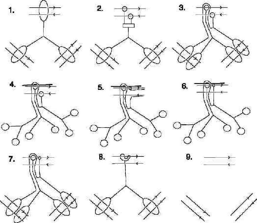
We now give the explanation of the figure. First, the two leaves which bound surfaces are the leaves at the bottom of frame 1. When constructing these surfaces we can assume that they run parallel to only one of the strands going through the top leaf. Let this strand be the top strand of the picture. Going to frame 2 is Habiro’s move $8$ . Going to frame $3$ follows easily from Habiro’s move 11. In frame $4$ we have added the two surfaces to the tips of one of the claspers. Rather than drawing the details, we have represented things schematically. The heavy line at the top of the picture reminds us that pieces of the new clasper run through here. In frame $5$ we have slid one of the leaves along the knot until it is opposite the other leaf. Because of the fact that the strands were oriented oppositely, the leaves face each other as shown. Going to frame $6$ is where we use the $\mathcal{S}_{5}$ move. We pull the edge of the clasper which is incident to the leaf we just slid into the shown position. Then by Lemma 3.9(b), the knots in pictures $5$ and $6$ cobound an $\mathcal{S}_{5}$ grope. To get to frame $7$ we forget the fact that there are surfaces bounding two of the leaves. (Basically the inverse of $3\to 4$ .) In frame $8$ we do Habiro’s move 11 in reverse. But then we have a clasper with trivial leaf, which does not alter the knot as in frame $9$ . ∎

Note that Corollary 1.3 follows immediately, because by Theorem 4.2, $c_{3}\mod 2$ is an invariant of all class $5$ grope cobordisms.

This corollary is somewhat surprising. [MO] have proven that the only rational finite type $S$ -equivalence invariants are the coefficients of the Alexander-Conway polynomial. Recall that $c_{3}\mod 2$ is not an Alexander-Conway coefficient. Recently, Ted Stanford [S] discovered that $c_{3}\mod 2$ can be expressed as a polynomial in the Conway coefficients $c_{2}$ and $c_{4}$ . Hence all known finite type invariants of S-equivalence come from the Alexander polynomial.

We have classified the behavior of all capped and uncapped class $5$ trees but the following.

Problem 4.11.

What is $\mathcal{K}/(\mathcal{S}_{5})^{c}$ ?

Clearly a $(\mathcal{S}_{5})^{c}$ move must preserve $S$ -equivalence and also type $4$ Vassiliev invariants. Conjecturally this completely characterizes the move.

We close this section with a natural conjecture based on our low-degree calculations.

Conjecture 4.12.

$\mathcal{K}/\mathcal{T}$ only depends on the unrooted tree type of $\mathcal{T}$ .

5. Miscellaneous results

5.1. Null filtration of knots which bound a grope

In the first author’s Ph.D. thesis [C] (see also [C2]), the question of a knot bounding a grope is considered. This is much stronger than cobounding a grope with the unknot. In particular, if a knot bounds a grope of class at least three, the knot has trivial Alexander polynomial, whereas this is certainly not the case for the cobounding situation. The central result in [C] is the following:

Theorem 5.1.

If a knot $K$ bounds an embedded grope of class $k$ into $S^{3}$ , then Vassiliev invariants up to degree $\lceil k/2\rceil$ vanish on $K$ .

In fact the bounding of a grope is an extremely restrictive condition. This can be very well expressed in terms of the null filtration of [GR]. It is obtained by the usual alternating sum formalism by declaring a null clasper surgery on a Y to have degree one. Here the word “null” expresses the condition that the leaves of the clasper must have trivial linking numbers with the knot. It follows that to be null equivalent to the unknot (the case $k=3$ below) is the same as having trivial Alexander polynomial, at least in a homology sphere.

Proposition 5.2.

If a knot $K$ bounds an embedded grope of class $k$ in a $3$ -manifold $M$ , then the pair $(M,K)$ is $(k-3)$ -null equivalent to the unknot in $M$ .

Proof.

A knot bounding a grope of class $k$ can be obtained from the unknot $U$ by surgery on a rooted tree clasper of Vassiliev degree $k$ , where $U$ is a meridian to the root. In particular, the other leaves do not link $U$ .

Break the clasper into a union of $(k-1)$ Y’s. Surger the knot along the Y which contains the root. This leads to a union of $(k-2)$ Y’s, which the surgered knot links trivially. Now consider the alternating sum, surgering over all subsets of the Y’s. It is easy to see that surgery on any proper subset does not change the knot, because there will be leaves which bound embedded disks. Hence the alternating sum reduces to $(M,U)-(M,K)$ and since we did $(k-2)$ Y-surgeries, these two knots are $(k-3)$ -null equivalent. ∎

5.2. Grope cobordism and orientation reversal

Proposition 5.3.

Let $\rho$ be the map reversing a knot’s orientation. Then for every knot $K$ in the $k$ -th term $G_{k}$ of the grope filtration of $\mathcal{K}$ , one has

K\equiv(-1)^{k}\rho(K)\mod G_{k+1}.

One can filter the primitive Feynman diagrams by grope degree, and in the associated graded group, it is straightforward to show that $D=(-1)^{|D|}\rho(D)$ . Conjecturally the graded pieces of this group are isomorphic to $\mathcal{G}_{k}$ , in which case we’d be done. However, we can still mimic the Feynman diagram computation geometrically.

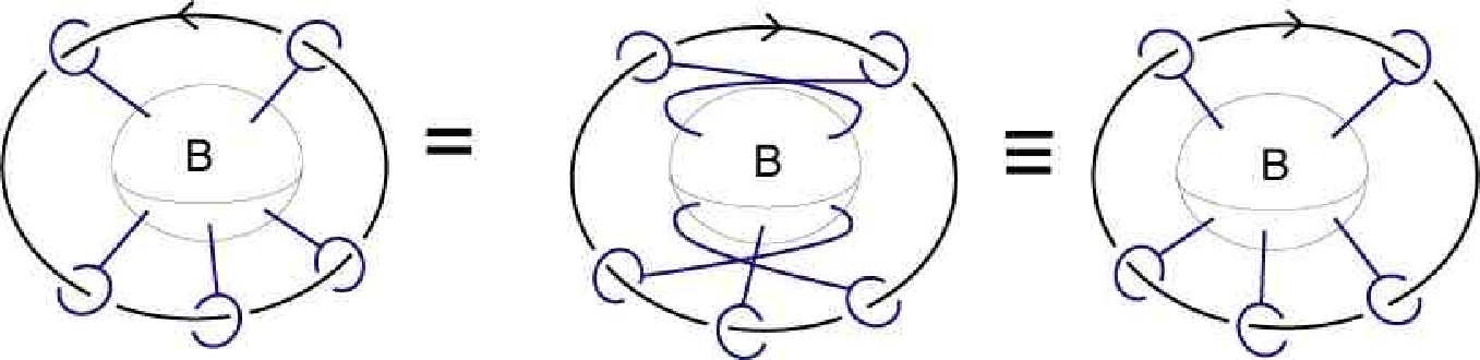
Proof of Proposition 5.3.

By Lemma 3.11(b) and Lemma 3.9(b), it suffices to show the result for $K=U_{C}$ , where $C$ is a simple clasper of degree $k$ which hits the unknot $U$ as on the left of Figure 12. Here $B$ is a ball which contains most of the clasper, excluding the leaves. One rotates the outer unknot about the vertical axis lying in the page, while keeping the ball $B$ fixed. By Lemma 3.9, we can reorder the leaves as on the right of the picture. Each edge incident to a leaf has picked up a half twist. Note that the parity of the number of leaves of a simple clasper matches the parity of the grope degree $k$ . By Lemma 3.11(a), we have shown that $U_{C}=(-1)^{k}\rho(U_{C})\in G_{k}/G_{k+1}$ . ∎

5.3. Simple clasper surgeries and the grope degree

In this section, we restrict attention to knots and claspers in 3-space. Consider the statement,

“A simple clasper surgery of degree $k$ may be realized by a sequence of simple clasper surgeries of degree $(k-1)$ .”

When the degree $k$ is the Vassiliev degree, this follows from Habiro’s work: By his main theorem any simple clasper surgery of Vassiliev degree $k$ may be realized by a sequence of simple tree clasper surgeries of Vassiliev degree $k$ . For a simple tree claspers, one breaks the clasper into a union of a degree $(k-1)$ tree clasper and a Y, with two leaves linking as a Hopf pair (exactly one of the leaves belongs to the Y). Surgering the knot along the Y, we get a capped tree clasper of Vassiliev degree $(k-1)$ , which can then be refined via the zip construction into a sequence of simple tree clasper surgeries of Vassiliev degree $(k-1)$ .

It is the purpose of this section to demonstrate that the above statement holds also for the grope degree.

Theorem 5.4.

A simple clasper surgery of grope degree $k$ may be realized by a sequence of simple clasper surgeries of grope degree $(k-1)$ .

We make the following preliminary definition for the purpose of this section.

Definition 5.5.

A clasper is said to be admissible if it is simple and the graph type is obtained from a connected trivalent graph with no separating edges by adding a positive number of legs to the edges. We also call the trivalent graph admissible.

Let $\mathcal{S}$ denote the set of finite sequences of connected uni-trivalent graphs with at least one univalent vertex. Consider the partial order generated by the relation

(G_{1},\ldots,G_{i},\ldots,G_{N})<(G_{1},\ldots,G_{i}^{1},G_{i}^{2},G_{i+1},\ldots,G_{N}),

where $G_{i}^{j}$ are the two other terms in an IHX relation involving $G_{i}$ . This partial order gives a convenient language to state the following lemma.

Lemma 5.6.

For all $s\in\mathcal{S}$ , there is an $s_{0}\in\mathcal{S}$ such that $s<s_{0}$ and $s_{0}=(G_{i})$ is a sequence of admissible graphs $G_{i}$ .

Proof.

Straightforward. ∎

The point is that these elementary relations can be realized topologically by embedded claspers, as the next proposition makes clear.

Proposition 5.7.

Let $G_{1},G_{2},G_{3}$ be uni-trivalent graphs related by an IHX relation, and let $C_{1}$ be a simple clasper of type $G_{1}$ , embedded in the complement of a knot $K$ . Then $C_{1}$ may be realized by a sequence of claspers one of which is of type $G_{2}$ , one of which is of type $G_{3}$ , and the rest of which have increased grope degree and (at least) the same number of simple caps.

Proof.

First, we must convert some edges of $C_{1}$ to Hopf pairs to obtain a tree clasper $\hat{C}_{1}$ of tree type $\hat{G}_{1}$ . This gives rise to induced tree types $\hat{G}_{2},\hat{G}_{3}$ . There is an inverse $\overline{C}_{1}$ to the clasper $\hat{C}_{1}$ inside a regular neighborhood of $\hat{C}_{1}$ . The leaves of the inverse are parallels of the original, but the edges may wander around the regular neighborhood in a complicated way. The edges do however avoid any caps that $\hat{C}_{1}$ may have.(See Lemma 2.9.) If $K_{1}$ is the knot after surgery on $C_{1}$ (equivalently on $\hat{C}_{1}$ ) then $\overline{C}_{1}$ sits on the knot $K_{1}$ , and surgery on it produces the original knot. The knot $K_{1}$ will wander through the Hopf pairs of $\overline{C}_{1}$ , but will link these leaves trivially. By Lemma 3.9(c), the surgery $\overline{C}_{1}$ can be realized modulo higher grope degree, by surgery along a clasper $\widetilde{C}_{1}$ obtained from $\overline{C}_{1}$ by pushing the knot out of the Hopf pairs.

Now we use the topological IHX relation, Theorem 3.10. There is a union of two tree claspers $\hat{C}_{2}$ and $\hat{C}_{3}$ in a regular neighborhood of $\widetilde{C}_{1}$ which are of type $\hat{G}_{2}$ and $\hat{G}_{3}$ respectively, such that surgery on $\widetilde{C}_{1}\cup\hat{C}_{2}\cup\hat{C}_{3}$ is null isotopic. The leaves of $\hat{C}_{2}$ and $\hat{C}_{3}$ are parallels of the corresponding leaves of $\widetilde{C}_{1}$ . The edges of $\hat{C}_{2}$ and $\hat{C}_{3}$ may run through the regular neighborhood of $C_{1}$ , but avoid any caps that $C_{1}$ may have.

Where there were Hopf pairs of leaves on $C_{1}$ , all the leaves of the three claspers link. However, these leaves of $\hat{C}_{3}$ have trivial linking number with $(K_{1})_{\widetilde{C}_{1}\cup\hat{C}_{2}}$ . Thus, by Lemma 3.9(c), $K_{1}=((K_{1})_{\widetilde{C}_{1}\cup\hat{C}_{2}})_{\hat{C}_{3}}$ is equivalent modulo higher grope degree to $((K_{1})_{\widetilde{C}_{1}\cup\hat{C}_{2}})_{\widetilde{C}_{3}}$ where $\widetilde{C}_{3}$ is a clasper obtained from $\hat{C}_{3}$ by pushing strands of the knot out of the Hopf pairs of leaves. Similarly, modulo higher grope degree $\hat{C}_{2}$ can be realized by a clasper $\widetilde{C}_{2}$ , where the knot has been pushed out of the Hopf pairs. Thus $K_{1}$ is equivalent modulo higher grope degree to $(((K_{1})_{\widetilde{C}_{1}})_{\widetilde{C}_{2}})_{\widetilde{C}_{3}}$ . However $(K_{1})_{\widetilde{C}_{1}}$ is equivalent modulo higher grope degree to $K$ . Hence $(K_{\widetilde{C}_{2}})_{\widetilde{C}_{3}}$ is equivalent modulo higher grope degree to $K_{1}$ . The claspers $\widetilde{C}_{2}$ , $\widetilde{C}_{3}$ have clean Hopf pairs, and when these are converted to edges, the resulting simple claspers have graph type $G_{2}$ and $G_{3}$ respectively.∎

Recall that a cap is an embedded disk bounding a leaf of a clasper $C$ , with interior disjoint from $C$ . If there are several caps, they are assumed to be embedded disjointly. A cap is simple (with respect to a knot $K$ ) if it has a single intersection with $K$ .

Definitions 5.8.

Let $C$ be a clasper having some caps.

(a)

Let $c_{1}(C)$ be the number of simple caps.
(b)

Let $g(C)$ be the grope degree of the clasper $C$ . After breaking some edges into Hopf pairs of leaves to make $C$ a tree clasper, $g(C)$ is the number of leaves minus one.

Lemma 5.9.

Consider a surgery on a clasper $C$ .

(a)
It may be realized by a sequence of surgeries on claspers $C_{i}$ which are of the following two possible forms.
- (i)
  
  $g(C_{i})=g(C)$ , $C_{i}$ is admissible, $c_{1}(C_{i})\geq c_{1}(C)$
- (ii)
  
  $g(C_{i})=g(C)+1$ , $c_{1}(C_{i})\geq c_{1}(C)$ .
(b)
If $C$ is admissible then the clasper surgery may be realized by a sequence of surgeries on claspers $C_{i}$ of the following two possible forms.
- (i)
  
  $g(C_{i})=g(C)-1$ , $c_{1}(C_{i})>c_{1}(C)$
- (ii)
  
  $g(C_{i})=g(C)$ , $c_{1}(C_{i})>c_{1}(C)$

Proof.

Part (a):

By Theorem 20 of [CT], we may realize $C$ by a sequence of simple clasper surgeries of the same grope degree and at least the same number of simple caps together with some surgeries of higher grope degree which have at least the same number of simple caps. (One must check that [CT] Lemma 19 does not decrease the number of simple caps. Some caps may be destroyed when adding the nested tubes at one stage of the proof. However, instead of adding the nested tubes, push the disk over the cap as we did for the root leaf.)

Hence it suffices to prove (a) for simple claspers. For a simple clasper $C$ , it is straightforward to show that there is a sequence of admissible graph types $s_{0}$ such that $s_{0}\geq(G)$ , where $G$ is the graph type of $C$ . Then we have $(G)\leq s_{1}\leq s_{2}\leq\ldots\leq s_{n}\leq s_{0}$ , where each sequence is related to the next by a replacement of a single graph by a pair related by IHX.

Proposition 5.7 implies that an elementary relation $s_{i}\leq s_{i+1}$ can be realized geometrically modulo higher grope degree. More precisely, if $s_{i}$ represents a sequence of clasper surgeries between a knot $K_{0}$ and $K_{1}$ , then there is a sequence of clasper surgeries of the form $s_{i+1}$ which also go between $K_{0}$ and $K_{1}$ . Therefore, we have that $C$ can be implemented, modulo higher degree, by a sequence of claspers of the form $s_{0}$ , which are admissible. This concludes the proof of part (a).

Part (b): Since the clasper is admissible, every univalent vertex is part of a Y, such that the two other vertices of the Y are trivalent, and there is a path connecting them which doesn’t hit the Y’s interior. Surger the knot along the Y. This gives a connected clasper which has two new capped leaves having two intersections with the knot each. Refining this clasper using Theorem 20 of [CT], we will get some claspers of higher grope degree and some simple claspers where some number of edges have been cut. All of the latter type have increased $c_{1}$ , since we took a single simple cap of the original and converted it to two simple caps in all the daughters. Cutting of edges will add even more simple caps. ∎

Lemma 5.10.

(a)

A clasper surgery of grope degree $(2k-1)$ is realizable by a sequence of simple tree clasper surgeries of grope degree $(k-1)$ .
(b)

A clasper surgery which has $k+1$ caps is realizable by a sequence of simple tree clasper surgeries of grope degree $(k-1)$ .

Proof.

The proofs of both of these facts use the main theorem of Habiro [H2], which is that if two knots have the same degree $(k-1)$ invariants, then they are related by a sequence of simple tree clasper surgeries of Vassiliev=grope degree $k$ . The fact that grope degree $(2k-1)$ clasper surgeries preserve type $k-1$ invariants is Theorem 3 of [C2]. For part (b), if a rooted clasper $C$ has $k+1$ caps, it must have $k$ non-root caps. Then there are $k$ groups of crossing changes on $K_{C}$ which correspond to pushing the knot out of the caps. Since surgery on a clasper which has a cap that does not intersect the knot is trivial, doing any collection of these $k$ groups of crossings will yield the knot $K$ . Hence $K$ and $K_{C}$ are $k-1$ -equivalent. ∎

Proof of Theorem 5.4.

Define a complexity function, ordered lexicographically as the triplet $(c_{1},g,a)$ where $c_{1}$ is the number of simple capped leaves, $g$ is the grope degree, and $a(G)$ is zero unless $G$ is admissible, in which case it is one. If $g\geq 2k-1$ or $c_{1}\geq k+1$ then by the previous lemma the surgery is realizable by simple grope degree $k-1$ surgeries and we are done.

We prove the following statement by contradiction: “Every clasper surgery of grope degree $\geq k-1$ is realizable by a sequence of simple clasper surgeries of grope degree $(k-1)$ .”

Assume $C$ is a counterexample. Then, as noted above, $C$ lies inside the range $c_{1}\leq k$ and $k-1\leq g\leq 2k-2$ . Hence it makes sense to take $C$ to have maximal complexity $(c_{1},g,a)$ . There are two cases: either $g(C)=k-1$ or $g(C)\geq k$ . In the former case, $C$ cannot be admissible, since it would then be simple and hence not a counterexample. Therefore, $a=0$ , in which case Lemma 5.9(a) says that $C$ can be realized by claspers with higher complexity. Since $C$ is a counterexample, one of these daughters must also be a counterexample. But this contradicts that $C$ was of maximal complexity.

So we are left with the case that $g(C)\geq k$ . If $a=0$ , then as above Lemma 5.9(a) furnishes a contradiction. Otherwise, $a=1$ and so Lemma 5.9(b) says that $C$ can be realized by claspers of degree $\geq k-1$ , and of higher complexity. As before, this contradicts the maximality of $C$ . ∎

References

[Aa] D. Bar-Natan, S. Garoufalidis, L. Rozansky and D.P. Thurston The Aarhus integral of rational homology 3-spheres II: Invariance and universality, math.GT/9801049, to appear in Selecta Mathematica.
[BN] D. Bar-Natan, On the Vassiliev knot invariants, Topology 34 no. 2, 423-472
[Co] T. Cochran, Derivatives of links: Milnor’s concordance invariants and Massey’s products, Mem. Amer. Math. Soc. 84 no. 427, 1990.
[COT] T. Cochran, K. Orr and P. Teichner, Knot concordance, Whitney Towers, and $L^{2}$ -signatures, math.GT/9908117, to appear in the Annals of Math.
[CoT] T. Cochran and P. Teichner, Von Neumann $\eta$ -invariants and grope concordance, in preparation.
[C] J. Conant, A knot bounding a grope of class $n$ is $\lceil\frac{n}{2}\rceil$ -trivial, math.GT/9907158
[C2] J. Conant, On a theorem of Goussarov, to appear in J. Knot Theory Ramifications
[CST] J. Conant, R. Schneiderman and P. Teichner, A topological IHX relation in three and four dimensions, in preparation.
[CT] J. Conant and P. Teichner, Grope cobordism of classical knots, math.GT/0012118
[G] M. Goussarov (Gusarov), On $n$ -equivalence of knots and invariants of finite degree, Topology of Manifolds and Varieties, Adv. Sov. Math., vo. 18, Amer. Math. Soc., 1994, 173-192
[GR] S. Garoufalidis and L. Rozansky, The loop expansion of the Kontsevich integral, abelian invariants of knots and $S$ -equivalence, math.GT/0003187, to appear on Topology.
[GL] S. Garoufalidis and J. Levine, Concordance and 1-loop clovers, math.GT/0102102
[GGP] S. Garoufalidis, M. Goussarov and M. Polyak, Calculus of clovers and finite type invariants of 3-manifolds, Geom. Topol. 5 (2001), 75-108
[GT] S. Garoufalidis and P. Teichner, On Knots with trivial Alexander polynomial, math.GT/0206023.
[H1] K. Habiro, Claspers and the Vassiliev skein modules, preprint 1999.
[H2] K. Habiro, Claspers and finite type invariants of links, Geometry and Topology, vol 4 (2000), 1-83
[M] S.V. Matveev Generalized surgery of three-dimensional manifolds and representations of homology spheres, Math. Notices Acad. Sci. USSR, 42:2 (1987) 651-656
[MN] H. Murakami and Y. Nakanishi, On a certain move generating link-homology, Math. Ann. 284 (1989), no. 1, 75-89.
[MO] H. Murakami and T. Ohtsuki, Finite type invariants of knots via their Seifert matrices, math.GT/9903069
[NS] S. Naik and T. Stanford, A move on diagrams that generates S-equivalence of knots, math.GT/9911005
[Ng] K.Y. Ng, Groups of ribbon knots, Topology 37, 441-458.
[S] T. Stanford, private communication.
[T] D.P. Thurston, Wheeling: A diagrammatic analogue of the Duflo isomorphism, Ph.D. Thesis, UC Berkeley, 2000

Grope cobordism and Feynman diagramsThanks: The first author was partially supported by NSF VIGRE grant DMS-9983660. The second author was partially supported by NSF grant DMS-0072775 and the Max-Planck Gesellschaft.

Abstract.

Key words and phrases:

1991 Mathematics Subject Classification

1. Introduction

Theorem 1.1.

Proposition 3.8 .

Challenge .

Theorem 1.2.

Corollary 1.3.

Challenge .

Proposition 5.2 .

Proposition 5.3 .

Theorem 5.4 .

2. Gropes, claspers and diagrams

2.1. Basic notions

2.2. Feynman diagrams

2.3. Maps relating capped gropes and Feynman diagrams

Lemma 2.1.

Lemma 2.2.

2.4. Clasper forests and Feynman diagrams

Definitions 2.3.

Lemma 2.4.

Lemma 2.5.

Proof.

Lemma 2.6.

Proof.

Proposition 2.7.

Proof.

Lemma 2.8.

Proof.

Lemma 2.9.

Proof.

Lemma 2.10.

Proof.

Corollary 2.11.

Proof.

Lemma 2.12.

Proof.

Lemma 2.13.

Remark 2.14.

Proof of 2.13.

3. The grope degree

Definition 3.1.

3.1. Feynman diagrams and the grope degree

Lemma 3.2.

Proposition 3.3.

Proof.

Definition 3.4.

Corollary 3.5.

Proof.

Lemma 3.6.

Proof.

Corollary 3.7.

Proof.

3.2. 4-dimensional grope cobordism: Grope concordance

Proposition 3.8.

Proof.

3.3. Clasper moves and the grope degree

Lemma 3.9.

Proof.

Theorem 3.10 ([CST]).

Lemma 3.11.

Proof.

4. Low degree calculations

Proposition 4.1.

Proof.

4.1. The groups 𝒦/Gk\mathcal{K}/G_{k} for k≤5k\leq 5

Theorem 4.2.

Lemma 4.3.

Definition 4.4.

Proof of 4.2.

Conjecture 4.5.

Proposition 4.6.

Proof.

4.2. Tree types of class 44

Proposition 4.7.

Proof.

4.3. Tree types of class 55

Lemma 4.8.

4.1. The groups $\mathcal{K}/G_{k}$ for $k\leq 5$

4.2. Tree types of class $4$

4.3. Tree types of class $5$

4.4. $S$ -equivalence