The Bernstein problem in the Heisenberg groupThanks: The first author was supported by NSF grants No. DMS-0070492 and No. DMS-0300477Thanks: The second author is partially supported by NSF grants No. DMS-9971563 and No. DMS-0306752
Abstract.
We establish the following theorem of Bernstein type for the first Heisenberg group : Let be a connected -minimal surface which is a graph over some plane , then is either a non-characteristic vertical plane, or its generalized seed curve satisfies a type of constant curvature condition.
1. Introduction
The development of last century’s mathematics has been enormously influenced by the desire to understand minimal surfaces. In such development the Bernstein problem has played a central role. The latter states that a smooth complete minimal graph in , i.e., a entire solution of the minimal surface equation
| (1.1) |
must necessarily be an affine hyperplane. Bernstein himself [Be] established this property when . Almost fifty years later Fleming [Fle] gave a completely different proof still for the case , and also conjectured that Bernstein result should be valid in any dimension. His approach inspired a new major development in the subject. In [DG] De Giorgi was able to extend Bernstein’s theorem to the case . Almgren [Al] subsequently succeeded in treating the case , and Simons [Sim] finally obtained a solution for . In their celebrated work [BDG] Bombieri, De Giorgi and Giusti established the surprising result that the Bernstein property fails if , thus putting an end to the problem in Euclidean space. They proved in fact that: if there exist complete minimal graphs in which are not hyperplanes. For additional references and developments the reader should also consult [O], [N1], [G], [MM], [Bo], [N2], [Si], [GMS], [CM].
The main objective of this paper is investigating the Bernstein problem in the first Heisenberg group . This is the simplest and most important non-Abelian model of a class of graded, nilpotent Lie groups known as Carnot groups. Such groups arise naturally as tangent spaces to sub-Riemannian manifolds, also known as Carnot-Carathéodory spaces, see [F], [St], [Bel], [Gro1], [Gro2], [Mon], [G]. For , the underlying manifold of the Heisenberg group is , with group law
| (1.2) |
Here, we have let , , . Denoting by the left-translation associated with (1.2), and by its differential, one readily recognizes that the generators of the (real) Heisenberg algebra are the left-invariant vector fields
| (1.3) |
. The sub-Laplacian on is the second-order partial differential operator given by . Such operator is the real part of the Kohn sub-Laplacian in , see [St]. One has
| (1.4) |
where represents the characteristic direction, all other commutators being trivial. One can thus decompose the Heisenberg algebra as follows , with , , and since (1.4) implies , we see that Hörmander’s finite rank condition [H]
| (1.5) |
is fulfilled at step . The natural non-isotropic dilations on are , with corresponding homogeneous dimension . Noting that Lebesgue measure is a bi-invariant Haar measure on , one has in fact .
Minimal surfaces are surfaces of least perimeter, or area, among all those with the same boundary. In a Carnot-Carathéodory space an appropriate sub-Riemannian version of perimeter generalizing the classical one due to De Giorgi was introduced in [CDG], and further developed in [GN], see also the papers [BM] and [FSS1] where two equivalent definitions were independently set forth. To provide the reader with a broader perspective of the results in this paper, it may be useful to recall the relevant definitions in the setting of a Carnot group with a given subbundle , and a distribution of smooth vector fields which is bracket-generating for . Given an open set , we let
For a function , the -variation of with respect to is defined by
A function is called of bounded -variation in if . The space of functions with bounded -variation in , endowed with the norm
is a Banach space. Let be a measurable set, be an open set. The -perimeter of with respect to is defined by
| (1.6) |
where denotes the indicator function of . An -minimal surface in an open set was defined in [GN] as the boundary of a set of least -perimeter, among all those with the same boundaries outside . The existence of such surfaces and a measure theoretic solution of the corresponding Plateau problem were established in [GN].
In this paper, we do not study -minimal surfaces from the geometric measure theoretic viewpoint, but rather follow the classical development of the subject. For us, an -minimal surface will be a hypersurface whose horizontal mean curvature , see Definition 1.1, vanishes everywhere. This notion of a minimal surface was independently introduced in [DGN2] and [Pau], and the present paper was inspired by these works. Of course, the concept of horizontal mean curvature plays a central role here. Just as the Gauss map guides the theory of Euclidean minimal surfaces, the horizontal Gauss map dominates the study of -minimal surfaces. To define this notion, we suppose that has been endowed with a left-invariant Riemannian metric with respect to which constitute an orthonormal basis. Here, the vector fields , defined in (1.3), span the horizontal subbundle . We consider an oriented surface and let be the Riemannian unit normal to the surface. We define the horizontal normal , relative to the basis of , by the formula
The horizontal Gauss map is defined by
| (1.7) |
at every point of the set . The following definition was introduced in [DGN2].
Definition 1.1.
The -mean curvature (or horizontal mean curvature) of at points of is defined by
where , indicate the tangential horizontal derivatives, see Definition 2.2.
A surface is called -minimal if it has -mean curvature equal to zero. It may be helpful for the reader to know that there exists a close connection between such notion of minimal surface and the geometric measure theoretic one introduced in [GN]. One has in fact the following first variation formula (see Theorem 10.2 in [DGN2]). Let be a surface with characteristic set , and suppose that . Consider the family of surfaces , where for small we have let
| (1.8) |
The first variation of the -perimeter with respect to the deformation (1.8) is given by
| (1.9) |
where as in (2.3) we have denoted with a defining function for , is the angle function defined in (2.11), and denotes the Borel measure induced on by the -perimeter defined in (1.6). In particular, we conclude from (1.9) that: is stationary with respect to (1.8) if and only if it is -minimal.
In [Pau], the second author used the approximation of by Riemannian manifolds (in the Gromov-Hausdorff topology) to characterize and investigate the solutions of the minimal surface and Plateau problems in via approximations by solutions to the analogous problems in the approximating Riemannian manifolds. In [DGN2], D. Danielli, the first named author, and D.M. Nhieu developed a sub-Riemannian calculus for hypersurfaces in Carnot groups. In [DGN1] they also determined, under some conditions, the isoperimetric sets in the Heisenberg group, i.e., those bounded sets which minimize the -perimeter under a volume costraint, and they proved that their boundaries are (but not !) hypersurfaces with positive constant -mean curvature. In the same paper the following sub-Riemannian Bernstein problem was formulated: consider a complete -minimal surface . Under which assumptions on and is it true that must be a vertical hyperplane, i.e., there exist , and , such that
| (1.10) |
One easily recognizes that the vertical hyperplanes in (1.10) are -minimal (however, any hyperplane in is -minimal. In particular, such is the characteristic hyperplane ). The following conjecture was proposed.
Conjecture: In the Heisenberg group , at least in low dimension, the Bernstein property should hold provided that the surface is an entire graph, and has empty characteristic locus. In particular, suppose that is a entire graph in the first Heisenberg group , and assume that has empty characteristic locus, then must be a vertical plane. I.e., there exist , with , such that
We recall that, given a hypersurface , a point is called characteristic if the vector fields (1.3) which generate the horizontal subbundle become tangent to at , i.e., . The collection of all the characteristic points of is called the characteristic locus of . We note explicitly that the set introduced above is given by .
Some comments concerning the above conjecture are necessary. Substantial evidence seems in favor of it. On one hand, there is the close relation between the Bernstein property and the classical Liouville theorem for harmonic functions. Such connection continues to hold in the sub-Riemannian setting. Now, the Liouville property in presents a striking new phenomenon with respect to the classical setting, namely that if is a bounded entire solution of the sub-Laplacian in , then depends only on the horizontal variables . As a consequence, such a function must, in fact, be an ordinary harmonic function in , and therefore by the classical Liouville theorem it is constant. Secondly, and perhaps more importantly, a basic result in [FSS2] shows that when one adapts De Giorgi’s method of the blow-up to the sub-Riemannian setting of , one obtains in the limit blow-up sets which are vertical (non-characteristic) planes as in (1.10). By imposing the non-characteristic assumption in the conjecture one rules thus out the undesired -minimal characteristic hyperplanes such as .
In light of this evidence, our inital efforts went in the direction of proving the conjecture true. In the process of establishing its veracity, we have developed a basic representation result for a graph-like -minimal surface which is based on the notions of seed curve and height function, see Theorem A. While analyzing the various possibilities, however, we have made the striking discovery that the above conjecture is in fact not true.
Counterexample to the conjecture: The real analytic surface
| (1.11) |
is an entire -minimal graph, with empty characteristic locus, over the coordinate -plane in .
This counterexample, which will be analyzed in detail in Sections 3 and 6, shows the failure of the above formulated sub-Riemannian counterpart of the classical Bernstein property. Nonetheless, in this paper we prove a result, Theorem C, which we feel is in fact closest in spirit to the classical theorem of Bernstein. To precisely state this theorem, we first introduce some definitions, and present some results of independent interest which are fundamental in the proof of the main theorem.
To study -minimal surfaces, we form a set of coordinates which are adapted to the horizontal Gauss map on portions of the surface which are graphs over a domain in the -plane. In this sense, they are analogous to isothermal coordinates on minimal surfaces in . Roughly, for an -minimal surface written as a graph for a function over a domain of the -plane where has empty characteristic locus, we consider the unit horizontal Gauss map (1.7) of this surface. Setting and , we have
As the -minimal surface in question is a graph over the -plane, we have , , and thus the horizontal Gauss map on depends in fact only on the variables . By abuse of notation we write , and identify this function with the unit vector field over
| (1.12) |
Henceforth in this paper, we routinely identify with the point . Also, for , we let .
Definition 1.2.
Given a point , a seed curve based at of the -minimal surface is defined to be the integral curve of the vector field with initial point . Denoting such a seed curve by , we then have
| (1.13) |
If the base point is understood or irrelevant, we simply denote the seed curve by . We will indicate by the integral curve of starting at the point .
We note explicitly that, thanks to , a seed curve is always parameterized by arc-length. Using as our coordinate curves, we obtain a new local parameterization of the -plane , given by
| (1.14) |
Keeping in mind that, from (1.13), , we have
| (1.15) |
As we will see in Section 4, defines a local diffeomorphism over a region of the -plane, up to a certain curve , see Lemma 4.5.
Our first result is a basic representation theorem for -minimal surfaces with empty characteristic locus which are graphs over a portion of the -plane.
Theorem A.
A patch of a surface of the type
where is a function over a domain in the -plane, and with empty characteristic locus over , is an -minimal surface if and only if for every , there exists an open neighborhood of on that can be parameterized by
| (1.16) |
where is given by
| (1.17) |
with
Thus, to specify such a patch of smooth -minimal surface, one must specify a single curve in determined by a seed curve , parameterized by arc-length, and an initial height function .
One consequence of the representation in Theorem A is that -minimal surfaces are, in fact, ruled surfaces. In particular, for fixed , the straight line in the -plane lifts to a straight line on which is a geodesic in , see Corollaries 5.1 and 5.3. We stress that Theorem A is useful in both the study of known examples as well as in the construction of new -minimal surfaces. Indeed, in Sections 6 and 9 we demonstrate the construction of new types of surfaces, see Examples 6.5, 6.6, 6.7, and Example 9.5. We also stress that the counterexample given above was discovered in a similar way.
Seed curves associated to -minimal surfaces are our fundamental objects of study. With this in mind, we introduce the following definition.
Definition 1.3.
If no portion of a , complete, connected -minimal surface can be written as a graph over the -plane, we say that has trivial seed curve. Otherwise, has a non-trivial seed curve.
In this definition and subsequent theorems, we will use the term complete surface to denote a metrically complete open surface in the Heisenberg group.
We show in Lemma 4.9 that if has trivial seed curve, then must be a vertical plane as in (1.10). However, to completely describe an -minimal surface we need to suitably extend to notion of seed curve. A generalized seed curve is a collection of seed curves and associated height functions together with patching data which define a single curve in , see Definition 9.2.
The next theorem shows that generalized seed curves completely determine -minimal surfaces.
Theorem B.
Let be a , complete, connected -minimal surface. Then, either is a vertical plane, or is determined by a generalized seed curve.
In the following definition the signed curvature of a seed curve is that given in (4.13) of Definition 4.4.
Definition 1.4.
An -minimal surface is said to have constant curvature if either it has trivial seed curve (in which case is a vertical plane), or if the signed curvature of each seed curve which is part of the generalized seed curve defining the -minimal surface is constant.
We emphasize two important points concerning this definition. First, that the assumption of constant curvature does not imply that the curve in defined by the generalized seed curve, , has constant curvature, merely that the seed curves, , do. Indeed, Example 9.5 explicitly shows this: each of its seed curves are straight lines (constant curvature zero) but the lifted curves, do not have constant curvature. Second, we point out that the individual seed curves, , for an -minimal surface of constant curvature may have different signed curvatures for different . A method to construct examples of such behavior is described after Definition 9.6.
We can now state our main result.
Theorem C (of Bernstein type).
Let be a connected -minimal surface which is a graph over some plane , then has constant curvature according to Definition 1.4.
When the complete -minimal surface fails to be a graph, then it need not have constant curvature. An example is given by the sub-Riemannian catenoids in Examples (3.4), (6.3). We stress that in the Theorem C we have made no assumption concerning the characteristic locus of . Theorem C points out a rigidity of the seed curve under the assumption that the -minimal surface is a graph: it must be composed of circles or lines. In the case where all the seed curves in the generalized seed curve are circles, may or may not have empty characteristic locus. However, in the case where at least one seed curve in the generalized seed curve is a straight line, we see that by (2) in Remark 7.2, always has non-empty characteristic locus. We stress, however, that there are many graph-like -minimal surfaces given simply by specifying different initial height functions. For instance, the -minimal surface (1.11) in the counterexample above, is a graph over the -plane, it has empty characteristic locus, see Example 3.5, and as we show in Example 6.4 its generalized seed curve consists of a single seed curve which is a circle. The plane is a graph over the -plane, it has non-empty characteristic locus, and again its single seed curve is a circle, see Example 6.1. On the other hand, we will construct a surface which is a graph over the -plane, has non-empty characteristic locus and seed curve a straight line, see Examples 3.2 and 6.2. In connection with this latter example, if we further restrict our attention to graphs over the -plane, then we can completely classify the possible -minimal surfaces.
Theorem D.
Suppose is a connected -minimal graph over the entire -plane, then:
- (1)
Either has seed curve a circle, and is a plane of the form for some real numbers , with , (with characteristic locus ).
- (2)
Or, has seed curve a straight line, and can be written as
where is a point in and are constants so that .
We note that, if we left translate so that the point is moved to the origin and further compose with an appropriate rotation about the -axis, we can write these surfaces as:
In addition, we note that the both of these classes of surfaces were found in [Pau], and, after the appropriate changes to reflect the difference in the representation of the Heiseneberg group, the second set of examples can be written as
for some real number , and some function (which is of course equivalent to the choice of ).
We mention in closing that Theorem D has been first established in the recent paper [CHMY], but with a completely different approach from ours. Besides Theorem D, the paper [CHMY] contains several other interesting results and also deals with the Heisenberg group from the broader perspective of three-dimensional CR manifolds. The analysis in [CHMY] is based on a detailed study of the characteristic locus of , whereas our approach is centered on the concepts of seed curve and height function. It is perhaps worth mentioning that we received from the authors the preprint [CHMY] on June 23, 2003, when the present paper was already undergoing an extensive revision with respect to its first version, in which we attempted to establish the above mentioned conjecture. At that time, in some email exchanges the authors of [CHMY] expressed to us their belief that our paper contained a flaw. This was caused by a misstatement of the main result in the abstract, which talked about minimal surfaces rather than minimal graphs. This unfortunate oversight led the authors of [CHMY] to incorrectly believe that we had missed the catenoid type example found by one of us (the latter was first described in [Pau] and is reviewed in Example 3.4). As the above discussion of the counterexample to the conjecture clarifies, the true reason for which our original attempt was flawed was in fact completely different, and it was brought to light by our discovery of the counterexample.
Acknowledgement: We would like to thank the anonymous referee for his/her constructive criticism and for several comments which contributed to improve the presentation of the paper.
2. The horizontal Gauss map and the minimal surface equation
In this section, we describe two notions of fundamental importance in the study of minimal surfaces in , the horizontal Gauss map, and the -mean curvature. To set the stage, we will suppose endowed with a Riemannian metric which makes an orthonormal basis, where the vector fields are given by (1.3), and as in (1.4) we have , all other commutators being zero. We consider an oriented hypersurface , and indicate with the Riemannian unit normal pointing outward. We recall is an orthonormal basis of the horizontal subbundle of the tangent bundle . We recall that the characteristic locus of is given by
| (2.1) |
Given a function on , its horizontal gradient is the projection onto the subbundle of its Riemannian gradient with respect to the orthonormal basis , i.e.,
Definition 2.1.
We define the horizontal normal , relative to the basis of the subbundle , by the formula
The horizontal Gauss map is defined by
whenever .
Throughout the following discussion we will denote by the natural domain of , i.e., the open set on
We note explicitly that is the projection of the normal on the horizontal subbundle , whereas is the normalized projection. An obvious, yet important consequence of the definition is
| (2.2) |
We next consider a function , where is an open subset of containing . The following notion, introduced in [DGN2], is central to the development of sub-Riemannian calculus on a hypersurface.
Definition 2.2.
At every point the tangential horizontal gradient of on with respect to the subbundle is defined as follows
In the next definition we introduce a sub-Riemannian analog of the classical notion of mean curvature.
Definition 2.3.
The -mean curvature of at points of is defined by
If we let
provided that such limit exists, finite or infinite. We do not define the -mean curvature at those points at which the limit does not exist.
Definition 2.4.
A surface is called -minimal if its -mean curvature vanishes everywhere.
It is interesting to write the -minimal surface equation in terms of a defining function for the hypersurface . Suppose that
| (2.3) |
where is , and there exists an open neighborhood of such that
We will think of as the boundary of the open set , so that the Riemannian outer unit normal to with respect to the orthonormal basis is given . One easily recognizes that in such case the horizontal Gauss map is given by
| (2.4) |
Thereby, the notion of -minimal surface introduced in [DGN2] coincides with that set forth in [Pau], and the corresponding minimal surface equation is given by
| (2.6) |
For a function we define the symmetrized horizontal Hessian of at as the matrix with entries
| (2.7) |
Setting , we introduce the matrix
| (2.8) |
The next proposition follows by a direct computation based on (2.5) and we leave the details to the reader.
Proposition 2.5.
At every point of one has
In particular, the -minimal surface equation for can be re-written as
| (2.9) |
It is standard to verify that the eigenvalues of are given by the equations
| (2.10) |
At non-characteristic points of we have . If we consider the -th entry of the vector , from the second equality in (2.8) we obtain
This proves that at points where , we have , so that is an eigenvector of with corresponding eigenvalue . From (2.10) we conclude that the second eigenvalue of is given by . One easily finds that an eigenvector for is given by . Thanks to , another eigenvector for is given by .
With an homage to classical notation, we now define
| (2.11) |
Moreover, for convenience we let
| (2.12) |
so that the minimal surface equation (2.6) becomes We also note the following useful equivalent form in terms of the functions and
| (2.13) |
We stress that if (2.6) is satisfied, i.e., if is -minimal, then from (2.9) and (2.10), we conclude that also , so that has a double eigenvalue equal to zero with a single eigenvector .
The expression of with respect to the variables is
| (2.14) |
With respect to these variables, the eigenvectors are (corresponding to eigenvalue ) and (corresponding to eigenvalue ).
Returning to Definition 2.1 we see that with respect to the variables and the horizontal Gauss map is given by
| (2.15) |
We end this section with a useful observation.
Lemma 2.6.
If in an -minimal surface in then any left-translation of is an -minimal surface. Moreover, any rotation of about the t-axis is also an -minimal surface.
The proof of this is a computation of the effect of left-translation and rotation about the -axis on the horizontal Gauss map coupled with the fact that the horizontal subbundle is preserved by both actions. The details are left to the reader.
3. Some examples of -minimal surfaces
In this section we analyze some interesting examples of -minimal surfaces. Most of the surfaces discussed in this section, with the notable exception of Example 3.5, are not new, as they have already appeared in [Pau]. However, the presentation in this section differs in spirit from that in [Pau] since it is organized having in mind the new ideas to be introduced in Section 4. In this sense, it should be viewed as preparatory to Section 6, where such new ideas will be illustrated in detail.
The reader should be aware that, throughout this section, and also in the rest of the paper, when a surface is given as a graph over a portion of the -plane, as in (4.1), we will identify the horizontal Gauss map, which is given by (2.15), with the two dimensional vector field defined in (1.12). Therefore, if sometimes we say that is equal to , we mean that such equation has to be interpreted through the identification . As we explain in the opening of Section 4 such identification is justified and also significantly aids in the computations.
Example 3.1.
Consider the characteristic plane . Using the defining function , and the equation (2.4), a simple computation shows that
The horizontal Gauss map is not defined at the characteristic point of . Nonetheless, one easily sees that
and therefore it is possible to define as a limit. This example is a special case of the following more general fact. Let
| (3.1) |
be an arbitrary plane in . When and , we obtain a vertical plane. We emphasize that such vertical planes have empty characteristic locus, with constant horizontal Gauss map coinciding with the Riemannian unit normal. Recalling (1.12) we thus obtain
When , the characteristic locus is composed of one single point , and for we have
| (3.2) |
In either case, it is readily recognized from (3.2) that
and therefore is a complete embedded -minimal surface. Incidentally, we notice the case also follows from the analysis of the characteristic plane , and by the left-translation invariance of the notion of -mean curvature. All one needs to observe is that by left-translating with respect to the point , one obtains the plane (3.1).
Example 3.2.
We next analyze the surface given by
| (3.3) |
with defining function . One has
and therefore the characteristic locus of is given by the -coordinate axis, i.e., . The horizontal Gauss map is well-defined in either of the two regions , . Furthermore, is constant on each region, and given by
| (3.4) |
It is immediately seen from (3.4) that
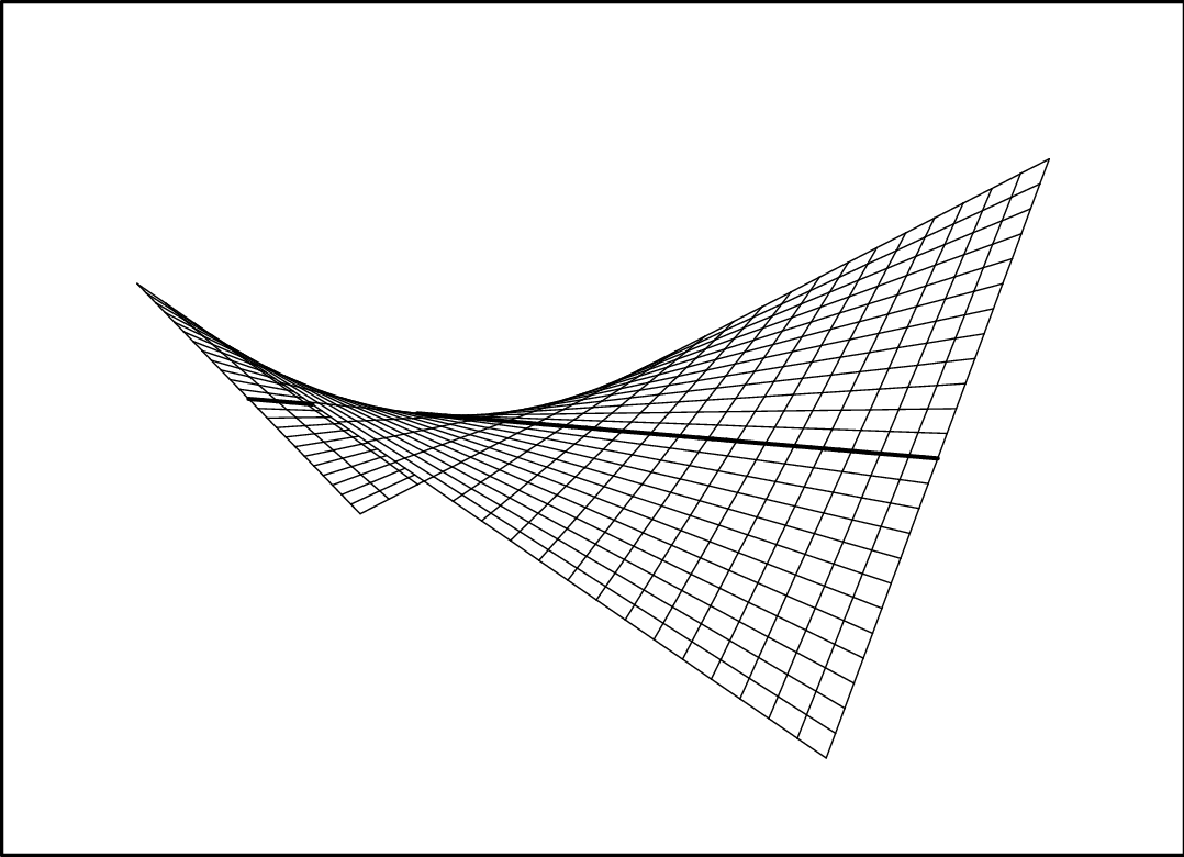
At points of the line , the -mean curvature can be defined as a limit. We thus conclude that on , and therefore is an entire -minimal graph over the -plane. Figure 1 shows a picture of this surface. The black line is the characteristic locus.
Before discussing the next example, we recall a useful result from [DGN2].
Proposition 3.3.
Let be a hypersurface in which is the level set of a defining function of the type
| (3.5) |
for some function . For every point point , such that , the -mean curvature at is given by
| (3.6) |
Using Proposition 3.3 it is possible to compute an interesting family of complete (globally defined) rotationally invariant -minimal surfaces in . Let us assume that be a hypersuface in described by a defining function as in (3.5). Using (3.6) for its -mean curvature, and imposing that , we find for
| (3.7) |
To solve (3.7) we multiply it by , and set , which gives , obtaining
This is a Bernoulli equation which is solved by the substitution , which yields
Returning to the dependent variable , we finally obtain
| (3.8) |
where and are arbitrary. If we specialize (3.8) to the case of , for which , we find
| (3.9) |
Substituting in (3.9), we obtain the following interesting conclusion.
Example 3.4.
The surfaces
are real-analytic complete -minimal surfaces in , with empty characteristic locus, which are not graphs on any of the three coordinate planes. They are the sub-Riemannian analogue of the classical catenoids. Thanks to (3.6), we see that satisfies the equation for every such that . Since does not intersect the -axis, we conclude that the -mean curvature vanishes everywhere on . The fact that has empty characteristic locus easily follows by the rotational symmetry of about the group center, the -axis, and by the fact that a surface with such property can only have characteristic points at the intersection with the -axis. Since such intersection is empty for , the conclusion follows. These surfaces where first discovered by the second named author, see Section 4.1.2 in [Pau]. The choice , and , yields the surface
which is represented in figure 2. Although we have already computed the -mean curvature using Proposition 3.3, it is nonetheless useful, for later purposes, to compute the horizontal Gauss map for such . Restricting attention to that portion of that lies above the plane , we can use the defining function
obtaining for projected horizontal Gauss map
| (3.10) |

Example 3.5.
The following example is quite striking, since it provides a (in fact, real analytic) -minimal surface which is an entire graph over the coordinate -plane, has empty characteristic locus, and which fails to be a vertical plane. Such example shows that the conjecture in the introduction fails to be true. Consider the surface
| (3.11) |
Clearly, (3.11) gives as an entire real analytic graph over the -plane. Figure 3 shows the surface as a graph over the -plane. Let us verify first that has empty characteristic locus . Using the defining function
we form
| (3.12) |
From the second equation in (3.12) it is clear that if , then and so has empty intersection with the plane . Suppose then that . In such case we see that if and only if
Now a simple computation gives
and therefore
| (3.13) |
Since the latter equation has no solution for , it is clear from (3.13) that , and thus . We next want to show that is -minimal. In this respect, it is easier to look at those patches of which can be written as a graph over the -plane. One easily recognizes that, on either side of the hyperplane , we can write the surface as follows
| (3.14) |
In this form, we take as defining function
obtaining
where we have let . From these formulas we obtain
| (3.15) | ||||
In the following computation it will be convenient to write , with . We see that
and therefore,
From these formulas we conclude
| (3.16) | ||||
Inserting (3.16) into (3.15), we conclude that on either of the two regions ,
. Since, as we saw from the representation (1.11), the characteristic locus of is empty, and therefore
the horizontal Gauss map is defined everywhere, we can extend by continuity to all of , thus concluding that such surface is globally -minimal.
We conclude the analysis of this example by writing explicitly the projection onto the -plane of the horizontal Gauss map when is expressed in the form (3.14)
| (3.17) |

We will return to the above examples in Section 6. To close this section we remark that, although all the above examples of -minimal surfaces are not just , but in fact real-analytic, due to the presence of characteristic points it is possible for a surface of constant -mean curvature to have only a fixed amount of regularity. As an instance of this negative phenomenon, we recall the following (partial) solution of the isoperimetric problem in established in [DGN2]. Consider the collection of sets , where
- (i)
;
- (ii)
There exist , and functions , satisfying , such that and .
Theorem 3.6.
Given , the variational problem
has a unique solution . Furthermore, is given explicitly as the graph
| (3.18) |
The sign depends on whether one considers , or . Finally, the set is only of class near its two characteristic points , it is away from them, and the compact hypersurface without boundary has positive constant -mean curvature given by
The isoperimetric sets (3.18) are surfaces of positive constant -mean curvature. It is natural to ask whether it is possible to construct surfaces of zero -mean curvature which are , but not better than that. In Section 6 we will show how to construct such -minimal surfaces, see Examples 6.5 and 6.6.
4. A representation theorem for -minimal graphs over the -plane
In this section, we consider an a priori special case, where we have an open set , and a function such that
| (4.1) |
With , we will assume that , where , so that the outward Riemannian unit normal to is given by
| (4.2) | ||||
We recall that has been endowed with a left-invariant Riemannian metric with respect to which constitute an orthonormal basis. We note that if we let , then the characteristic locus of is given by . As is a continuous function, we note that the characteristic locus is a closed set on the surface.
Re-writing the functions defined in (2.11) for the present situation, we have
| (4.3) |
where we have denoted . Moreover, since from (4.3) we see that , do not depend on , the minimal surface equation (2.13) presently reads
| (4.4) |
where is the usual divergence operator on and is the projection of the horizontal Gauss map defined in (1.12). Thus, minimal surfaces of this non-parametric type correspond to divergence free unit vector fields on . This observation leads us to introduce the following definition.
Definition 4.1.
Given a point , a seed curve based at of the -minimal surface of the type (4.1) is defined to be the integral curve of the vector field with initial point . Denoting such a seed curve by , we then have
| (4.5) |
We note explicitly that, thanks to , a seed curve is always parameterized by arc-length, and so . If the base point is understood or irrelevant, we simply denote the seed curve by . We will indicate by the integral curve of starting at the point , i.e.,
| (4.6) |
We now use some elementary analysis to investigate the types of planar vector fields such as and .
Lemma 4.2.
If is a , unit, divergence free vector field on , then the integral curves of the perpendicular vector field are straight lines.
Proof: An integral curve of satisfies the system
| (4.7) |
Letting , we find from (4.7)
| (4.8) |
Since is assumed to be unit, by differentiating the equation with respect to and we obtain
| (4.9) |
Since is also divergence free, we have
| (4.10) |
If we use (4.11) in (4.8) we conclude that , i.e., the vector field is constant along its own integral curves, hence, in particular, . From the latter equality we conclude that the integral curves of are given by
| (4.12) |
hence they are straight lines in starting at , with .
Corollary 4.3.
Let be an -minimal surface of the type (4.1). Given a point , the integral curve of starting at is given by a straight line perpendicular to
Proof: The hypothesis that be -minimal guarantees that the vector field is divergence free, see (4.4), therefore applying Lemma 4.2 with we conclude from its proof that is constant along its integral curves, and that the latter are given by (4.12).
According to Definition 4.1 a seed curve starting at is represented by the equation
From the latter we see that, if the point is non-characteristic, then the assumption that be implies that the vector field be in a neighborhood of , and thereby from the regularity theory for solutions of ordinary differential equations we infer that is of class in a neighborhood of . More in general, is is of class , then if of class in a neighborhood of .
Definition 4.4.
We define the signed curvature of by
| (4.13) |
For later purposes we note that
| (4.14) |
Returning to Definition 4.1, if we use as our coordinate curves, we have a new local parameterization of the -plane given by
| (4.15) |
We note explicitly that maps the straight line into the seed curve , i.e.,
On the other hand, the straight line is mapped into the straight line passing through the base point of the seed curve and having direction vector , i.e.,
Thanks to Corollary 4.3 we thus recognize that . In particular, when we obtain from this identity
| (4.16) |
Formula (4.16) will be useful later in the section. Keeping in mind (4.5) we see that along the seed curve we have . One thus has the following explicit expression for
| (4.17) |
Since , clearly depends on the choice of the base point as well. However, since in our arguments such point will be fixed, we will routinely omit such dependence. As we observed above if is , then , and therefore in its domain. More in general, if is of class , then . We next point out that fails to be a diffeomorphism everywhere. In fact, (4.15) gives
| (4.18) |
Thus, we have shown the following lemma.
Lemma 4.5.
The mapping defined in (4.15) ceases to be a local parameterization of a surface, in the sense that is not invertible, along the curve in the -plane given by
where is the signed curvature of the seed curve .
Next, we impose the new coordinates (4.15) on the function in (4.2). Under the new parameterization, the surface in (4.1) is given by
| (4.20) |
at least on that portion of the -plane where the map defines a diffeomorphism. We stress that, henceforth in the paper, by abuse of notation we indicate
with similar understanding when we express any other function, originally defined on an open set of the -plane, in terms of the coordinates . Thus, for instance, has to be interpreted analogously. We are now ready to establish the main representation theorem for -minimal surfaces of the type (4.1), see Theorem A in the introduction.
Theorem 4.6.
Let . A patch of a surface of the type (4.1), with empty characteristic locus over , is an -minimal surface if and only if, for every , there is a neighborhood of which can be parameterized by
| (4.21) |
with given in the form
| (4.22) |
with
We conclude from this, and from (4.17), that the map is not only , but in fact . Thus, to specify such a patch of a smooth -minimal surface of this type, one must specify a single curve in determined by a seed curve , parameterized by arc-length, and an initial height function .
Proof: First, we prove the necessity of the representation (4.21), (4.22). Assuming is an -minimal graph over a domain in the -plane, with empty characteristic locus, pick a base point, with being its projection onto the -plane. Let be the integral curve of such that . Further, suppose that the domain of is the interval . Now, for a fixed , let
and let . By construction we have that, if , then maps onto , where is the portion of which is a graph over . Now, for any fixed , consider , i.e., the function restricted to a curve parameterized by . As the trace of such curve lies on the surface, its tangent vector must be perpendicular to the Riemannian normal to along the curve. For the subsequent calculations it might be helpful for the reader to keep in mind the following formula which gives the relation between the expression of a vector field in the rectangular coordinates of , and that with respect to the orthonormal basis ,
| (4.23) |
We first compute using the representation (4.20) of
| (4.24) |
where we have used (4.23) along with the fact that in the coordinates one has
| (4.25) |
The Riemannian unit normal on the surface is given by (4.2), which, according to (4.3) and (2.12), we can write as
| (4.26) | ||||
Since and must be orthogonal, we see that
| (4.27) | ||||
Thus, we have the equation
| (4.28) |
which implies that
Letting
| (4.29) |
we have the desired result that is described as in (4.21), with given by
which is (4.22).
We next want to show that , and that . Before doing this, however, we prove that is one-to-one, and hence is a diffeomorphism. To show this, we argue by contradiction, assuming that there exist two points in such that
| (4.30) |
Since is a graph, (4.30) implies . Also, according to (4.15), (4.16), (4.30) is equivalent to saying that . This implies that . We notice that the possibility and is excluded, since in view of (4.16), (4.30) can be re-written
| (4.31) |
which if would reduce to . Since , the latter equation is impossible, unless . We must thus have . Assuming this, if , then we have also . But then the two straight lines represented by and are parallel and therefore, unless they coincide, they cannot intersect in thus violating the assumption . However, they cannot coincide unless . If this happens (i.e., if and the two straight lines coincide) then the parametric curve would self-intersect () with equal tangents at the intersection point. Since this would contradict the fact that is a smooth embedded curve, we conclude that we must have . Again, this forces
| (4.32) |
since otherwise the two lines , would be parallel and therefore they could not possibly intersect. Finally, we observe that (4.32) is equivalent to saying .
Keeping in mind that , we conclude from (4.32) that we must have
Thus, (and hence ) cannot be continuous at the point . However, the non-characteristic assumption implies that is continuous on , and we have thus reached a contradiction. This proves that is one-to-one and onto. Since it is a local diffeomorphism as well, we conclude is a diffeomorphism of onto .
We now turn to proving that and . To this effect, we analyze the curve . Looking at the parameterization we have just shown, we have given as
As observed following Definition 4.1, if is then, away from characteristic points, is at least . Therefore, since from (4.29) we have , from the chain rule and the fact that , we conclude that as well. We want to show next that .
Remark 4.7.
Suppose is parameterized as in Theorem 4.6 by a single seed curve and height function. For a fixed , consider
We note that this curve is a re-parametrization of the integral curve of passing through . To see this, we observe that, proceeding as in the proof of Lemma 4.2, one can show that is constant along the straight lines given by , with fixed. Keeping in mind (4.17) we thus conclude that for any fixed , and for every , one has
For a fixed , we see that the image of
coincides with the image integral curve of through (see Remark 4.7). Let be this integral curve. Since
and
Let
then if we take , whereas if , then we choose to be any positive number. With such choice of it is clear that
for every , and therefore is simply a re-parameterization of the integral curve, . Again, as the surface is , we have that is at least as well. To show the desired regularity of , we will consider the defining function of the surface, , restricted to . Again, since the surface is , is times differentiable along . First, we differentiate with respect to .
Fixing sufficiently close to zero (so that ), we know that and so . Thus,
where, for example,
We recall that if is differentiable and is differentiable that must be differentiable as well. Thus, as is differentiable we have that is as well. Moreover, as is independent of , we can divide by yielding that is differentiable. As the function is infinitely differentiable in , for it to be differentiable in as well, each must be differentiable in . For example, must be differentiable in since . Considering , we note that
where and . We note that both and are differentiable. Moreover, since we have
Now, putting these together we have that
Since all of the functions on the left hand side of the equation are differentiable along , we have that is differentiable in and hence in . As, , this shows that is differentiable as well. In other words, if the -minimal surface is at least , then is at least and is at least .
If, in addition, we assume that the surface is , we have that
is differentiable times in . A straightforward (but somewhat tedious) calculation shows that this implies that .
We now prove the reverse implication. We assume that the surface is parameterized by (4.21), (4.22), i.e.,
where is as in (4.15), (4.17), is a curve parameterized by arc-length and . We then show that is a -minimal surface. To do this we will compute the horizontal Gauss map for and show that it is divergence free. We will calculate the and derivatives of the parameterization yielding two tangent vectors to the surface from which to compute the Riemannian normal.
As above, we obtain from (4.15) for the derivative
| (4.34) | ||||
where in the last equality we have used (4.23), and the equation . We note that (4.34) shows, in particular, that the vector is horizontal. We next compute the derivative of the new parameterization of . Keeping in mind the convention , using (4.23) we find
| (4.35) | ||||
To complete the proof, we need to calculate the divergence of , and prove that the latter vanishes identically. In order to obtain a convenient expression of , we note that taking the cross-product, with respect to the orthonormal frame , of the vectors and tangent to , we easily obtain
| (4.36) | ||||
The equation (4.36) yields the following claim.
Claim 1.
For such that
we let
We thus see that
points in the same direction as the Riemannian normal to and hence the horizontal Gauss map for is given by
| (4.37) |
Having established this, and recalling (4.25), a routine computation using the inverse function theorem and (4.18), (4.19), yields that
| (4.38) |
The last equality stems from the assumption that is parameterized by arc-length and hence is orthogonal to . In view of (4.4) we conclude that is -minimal, and this completes the proof.
Remark 4.8.
We note that, as we see from (4.35), if
| (4.39) |
for some , then the vector is horizontal. Since the other tangent vector to , , is always horizontal, see (4.34), we conclude that if the parameterization were extended to include such a point, the point is a characteristic point. When examining individual H-minimal surfaces in terms of seed curves and height functions, as we will in section 6, this equation is useful for determining the characteristic locus.
We end this section by noting that in a different case, opposite to the case of graphs over the -plane, the -minimal surfaces are still ruled surfaces.
Lemma 4.9.
If is a -minimal surface so that no portion of can be written as a graph over the -plane, then is a subset of a single vertical plane.
Proof: Suppose is given locally by . Then, since no portion of can be written as a graph over the -plane, we must have . Then, and is a ruled surface whose generators are straight lines perpendicular (in ) to a curve . Using the implicit function theorem in , we can locally write as either or . For , we have the patch of surface defined by
In this case, and
Using the assumption that is -minimal, we take the divergence of to find that
which gives . This shows that the planar curve must be a straight line and is constant. A similar computation yields the same conclusion in the case . Thus, surfaces of this type must be composed of pieces of vertical planes. As is , it must be a portion of a single vertical plane.
5. -minimal surfaces as ruled surfaces
In this section, based on the work in Section 4, we put forth a geometric interpretation of -minimal surfaces which can be written as a graph over a portion of the -plane. In what follows, we will indicate with the Carnot-Carathéodory distance in generated by the vector fields . In view of Theorem 4.6 we see that if is a -minimal surface of the type (4.1), with empty characteristic locus, then there exist , such that letting
and
we have
| (5.1) | ||||
where is the anisotropic dilation of , and we have indicated with the group law (1.2). We note explicitly that, since belongs to the horizontal plane passing through the origin (the -plane), we have
| (5.2) |
Corollary 5.1.
Definition 5.2.
A ruled surface in is a surface which is foliated by geodesics of . Such a geodesic is called a rule. A curve transverse to the foliation is called a directrix of the ruled surface.
Corollary 5.1 and the representation (5.1) yield a nice geometric characterization of -minimal surfaces.
Corollary 5.3.
is a portion of a non-characteristic -minimal graph over the -plane in , parameterized as in Theorem 4.6, if and only if it is a piece of a ruled surface where the rulings are all straight lines in .
Proof: The geodesics in the ruling are given by the curves defined by (5.3) in Corollary 5.1. Thanks to (5.1) such geodesic is a straight line in (identified with ). A directrix of the ruling is parameterized by
Remark 5.4.
Note that the directrix contains two pieces of information, the first two coordinates compose a seed curve for and the last coordinate yields the initial height function . If we were using completely classical nomenclature, we would call the curve a line of striction since the curve is orthogonally transverse to the rules.
Remark 5.5.
The results of this section can be extended in several directions. First, similar results hold for the analogue of non-parametric constant mean curvature surfaces in the Heisenberg group - they are ruled surfaces as well but are foliated by geodesics which are lifts of circles in the plane. Second, both of these results can be generalized to some more general Carnot groups. Third, some of the regularity assumptions can be weakened yielding similar representation results. These results and some of their applications will be addressed in a future paper.
6. Further analysis of the examples
At this point, it might be helpful for the reader to return to the examples of Section 3 with the purpose of explicitly computing their seed curves , the diffeomorphism , the signed curvature and their singular locus .
Example 6.1.
Consider the characteristic plane in Example 3.1, whose horizontal Gauss map is given by
For every the seed curve solves the system
It is easy to recognize that if solves this system, then it must be . Using this latter information we find that the seed curve is given by the circle
| (6.1) |
Keeping in mind that , from (4.13) we obtain
The singular locus in Lemma 4.5 is thus presently given by the straight line
and the map
defines a local diffeomorphism on either side of such line. Of course, fails to be globally one-to-one, however by suitably restricting the range of we obtain a global diffeomorphism. For instance, if we let
then defines a global diffeomorphism onto. Notice that in the present example we have , and therefore the height function defined by (4.29) is given by . We next use the equation (4.39) in Remark 4.8 to determine the characteristic locus of . Such equation presently reduces to
which admits the double root . Since the parameterization of with respect to the coordinates is given by
we conclude that the characteristic locus is given by the image of the line through such map. We readily see that , in accordance with what we found in the discussion of Example 3.1. Figure 4 shows the vector field , the seed curve (in black) and some representative rules (in grey) to help illustrate this example. Note that the origin corresponds, as shown above, to both the characteristic locus and the image of the singular locus.

From the same discussion, it is easy to construct the seed curves and the corresponding height functions for the more general characteristic planes (3.1) in the case . Recalling that such planes are obtained by left-translating with respect to the point , one easily recognizes from (3.2) that, given , the seed curve with initial point is given by
| (6.2) |
where represents the seed curve in (6.1) for the plane with initial point . It might be helpful to observe, in this respect, that
Example 6.2.
We next analyze the surface
given in Example 3.2. Recalling the expression (3.4) of the horizontal Gauss map, if for instance , then one readily verifies that the seed curve is a straight line given by
| (6.3) |
and therefore
From this we infer that the singular locus , and in fact
| (6.4) |
defines a global diffeomorphism of onto itself. In the coordinates the defining function of is expressed by
and therefore we find in particular
Imposing equation (4.39) we see that in the plane the characteristic locus is given by the straight line . The image of this line on the surface through the diffeomorphism (6.4) is given by the equation
in which we need to set . We thus obtain the collection of points
This is in accordance with the characteristic locus that we found in Example 3.2 in terms of the coordinates .
If, instead, , then the corresponding seed curve is the straight line given by
and the relative diffeomorphism and height function by
If we impose (4.39) with these data, we reach the same conclusion for the characteristic locus. In figure 5, we show the vector field , a seed curve corresponding to in equation 6.3 (in black) and some representative rules (in grey). We can see from the picture that the rules are all parallel, which provides visual confirmation of the fact that the singular locus is empty.

Example 6.3.
We consider here the sub-Riemannian catenoids in Example 3.4, in which we choose , and . Such choice yields the surface
We restrict attention to that portion of that lies above the plane , for which the corresponding horizontal Gauss map is given by (3.10). Denoting with , we fix a point and compute the corresponding seed curve . The latter solves the system
| (6.5) |
One recognizes that if is a solution to (6.5), then
and therefore
| (6.6) |
This shows that the seed curve of is similar to a spiral of Archimedes, and we have
Restricting to the range , we see that , and therefore it is legitimate to substitute (6.6) into (6.5), and the system reduces to the linear one
| (6.7) |
In figure 6 we again show , a seed curve in black and some rules in grey for one of these surfaces, . Note that the vector field is not defined inside the circle of radius . We also note that this picture corresponds to the seed data for the upper half of the surface, the graph . There is a corresponding picture for the lower half resulting in a similar seed curve for the bottom portion of this surface. We note that, in this case, we need two seed curves to describe the surface completely as the surface has two sheets when written as a graph over the -plane. As with Example 9.5, this justifies the necessity of the notion of generalized seed curve that we introduce in Section 9.

Example 6.4.
We next analyze the surface in the Example 3.5. To compute a seed curve we will use the parameterization (3.14) of ,
| (6.8) |
which is valid over the open set . Recalling the corresponding expression (3.17) of the horizontal Gauss map, we see that for every the seed curve starting at must satisfy the system
| (6.9) |
As in the previous example we easily recognize that if solves (6.9), then it must be . With this information in hands, (6.9) reduces to
| (6.10) |
It is easily recognized that
and therefore (6.10) further reduces to
| (6.11) |
Incidentally, although the function no longer plays a role in (6.11), we note that its expression in the new coordinates is given by
The solution to (6.11), the seed curve , is given by the circle
From (4.13) we obtain, as in Example 6.1,
| (6.12) |
with singular locus given by the straight line
Outside of the map
| (6.13) | ||||
defines a local diffeomorphism, similarly to Example 6.1. Finally, we note that, in the coordinates , the function in (6.8) is given by
thus, in particular,
for
We now use (4.39) to verify, in conformity with what we found in the discussion of Example 3.5, that the characteristic locus of is empty. Since
(4.39) presently reads
It is clear that the latter equation has no solution in the region
and therefore . For instance, if , then (6.12) gives , and we find , with
In figure 7 we show a seed curve (in black) and some rules (in grey) for this example. We note that all the rules intersect at the origin, reflecting the fact that, in this case, the singular locus maps to a point in the -plane, the origin , see equation (6.13). By analyzing the equation of the surface, we see that, near the origin in the -plane, the surface ceases to be a graph over the -plane. We also note that there are portions of this plane where is not defined because the height function, , tends to for .

We next present two examples which demonstrate some of the restrictions on regularity of -minimal surfaces. We show how to construct a -minimal surface which is not , and whose characteristic locus is not smooth.
Example 6.5.
Let be a strictly positive, continuous, nowhere differentiable function, and let . We define a curve in the plane by letting
The function gives a curve parameterized by arc-length which we use as a seed curve for an -minimal surface, . Note that
and
and so (4.13) gives
We point out that, since , if we choose , the computations in the second half of the proof of Theorem 4.6 apply and this seed curve and height function pair define an H-minimal graph. Moreover, using (4.39), after picking , we can explicitly write down the characteristic locus. For example, if we take
then (4.39) gives for the characteristic locus
As is nowhere differentiable, we see that the characteristic locus is also nowhere differentiable. Moreover, by construction, the patch of given by the equations (4.21), (4.22), defined on the open set
is a graph over the -plane containing one branch of the characteristic locus, .
Example 6.6.
As a more concrete situation, we will consider the case where in Example 6.5. Of course, such is differentiable everywhere except at , but we will still produce a characteristic curve of the corresponding -minimal surface which is not differentiable at one point. Using the construction above, we have that in the plane the characteristic locus is given by the curve
Taking the branch

we see that the characteristic locus is not differentiable at . Indeed, letting , we have as , and therefore if we set , we find
and
The characteristic set of the -minimal surface is given by the image on , , via the parameterization (4.21), (4.22), of the curve ,
Direct computation shows
where
Figure 8 shows a picture of the characteristic locus - one can see the point of non-differentiability. Figure 9 shows a portion of the surface with the image of the seed curve in black and the characteristic locus in grey.

Example 6.7.
In most of the previous examples, we examined surfaces first discussed
in Section 3 as graphs over a portion of a coordinate plane, in terms of their seed curves and height
functions. While this brings a new perspective in the analysis of known -minimal
surfaces, here we wish to emphasize the usefulness of Theorem 4.6 in
the creation of new examples. Specifically, by simply picking a seed
curve and a height function, the representation given in Theorem
4.6 yields an -minimal surface. To illustrate this, we will
address the following question: do there exist -minimal surfaces
that are topological cylinders with piecewise constant horizontal
Gauss map? Here, we mean that , thought of as a vector field on
the plane, is piecewise constant. Of course, Example 3.4
gives an -minimal surface which is a topological cylinder, but its
unit horizontal Gauss map is not piecewise constant in this sense.
To answer this question, we recall that in the proof of Theorem
4.6, we showed that given an -minimal graph over the -plane, , with seed
curve and height function , the unit horizontal
Gauss map at a point is given by the vector .
Thus, if we wish to create a surface with constant unit horizontal
Gauss map, we need to pick to be a straight line. So, for any portion
of the desired surface which is a graph over the -plane, we must have
that the seed curve is a straight line.
Now, to form a topological cylinder, we will attempt to glue two such
-minimal graphs, and , together by picking appropriate initial height
functions. Experimentation yields the following solution: for we take and , while for we choose
and . In other words, we
pick straight lines for seed curves and lift them using appropriate
height functions so that when glued together they form a circle.
Applying the representation formula (4.21) in Theorem 4.6, we have
that is given by
and is given by
We may now use (4.22) to algebraically simplify the latter two equations to find that the surface is implicitly given by
We notice that is contained in the slab , and that its characteristic locus is given by the curve . If we let , , then we have on , on .
7. Characteristic points on -minimal graphs over the -plane
We turn next to understanding how characteristic points can arise on -minimal graphs. From the proof of Theorem 4.6, we see that for a -minimal surface which is a graph over a portion of the -plane, the characteristic locus corresponds to the equation
| (7.1) |
This formula, while explicit, is rather cumbersome. In this section, we will provide a slightly different perspective from which to view the characteristic locus which gives a different and admittedly only slightly less cumbersome formula, see Theorem 7.1 and Remark 7.2. However, this second formula will be much more useful in determining the characteristic locus.
Under the same assumptions outlined at the beginning of Section 4, we note that the (non-unit) Riemannian normal to the surface can be written as
| (7.2) |
see formula (4.26). We recall that the angle function is independent of , as we assume that is a graph over the -plane. The characteristic locus corresponds to those points where . The formula (7.1) gives one representation for such locus. For a different derivation, we use the Fröbenius condition to impose a restriction on . First, we observe that the -plane field perpendicular to is spanned by
To verify the assumption in Fröbenius’ theorem, we must impose the condition that for some . Now,
| (7.3) |
On the other hand, we have
| (7.4) |
The fact that are functions of and only allows us to simplify equation (7.5) as follows
| (7.6) |
or,
| (7.7) |
In other words, the directional derivative of in the direction of is . Since , we see from (4.37) that
Using this information, and the equations (4.38), we obtain
| (7.8) |
where in the latter equality we have used (4.13). Substituting (7.8) in (7.7), we conclude
| (7.9) |
We now recall the local diffeomorphism introduced in (4.15). In terms of the coordinates we see that
If we use this in combination with (7.9), we find
| (7.10) |
Solving this differential equation, one obtains the following result.
Theorem 7.1.
If the Riemannian normal to a -minimal graph over the -plane is given by (7.2), then
where . Moreover, for the characteristic locus of the -minimal surface is given by
Remark 7.2.
Several comments are in order:
- (1)
- (2)
If for some , then the characteristic locus of the surface must contain the point corresponding via the local diffeomorphism to the point in the -plane, where
- (3)
If , the characteristic locus has two components
one on each side of the point , with
- (4)
If , then the surface has no characteristic points along the rule passing through .
- (5)
If , then there is a single characteristic point at along the rule passing through .
Theorem 7.3.
Suppose . If the characteristic locus contains more than a single point, then the characteristic locus of a -minimal surface is a curve.
Proof: To determine the regularity of the characteristic locus, we first suppose that contains more than one point. If is the Riemannian unit normal to the surface, we may write the (closed) condition that defines characteristic points as (the reader should keep in mind that we have endowed with a left-invariant Riemannian metric with respect to which constitute an orthonormal basis). So, in a sufficiently small neighborhood of a characteristic point must be a graph over the -plane. Deleting the characteristic points from this neighborhood, we have an open non-characteristic patch of the surface and may use Theorem 4.6 to parameterize the patch using seed curves and height functions. Using Theorem 7.1, and (1) of Remark 7.2, we have that the characteristic locus is given by
| (7.11) |
where . As in the remarks after Theorem 7.1, we can describe the characteristic locus as . Using the implicit function theorem, we know that this curve is differentiable if equation (7.11) is differentiable in . By Theorem 4.6, we know that if then , and we have that the right hand side of (7.11) is times differentiable in as desired.
Remark 7.4.
The statement that a -minimal surfaces with characteristic locus larger than a single point is is also shown in Theorem B in [CHMY], although using different techniques.
8. Allowable gluing of patches of complete embedded -minimal surfaces
In the previous sections, we have discussed a local parameterization of -minimal surfaces near non-characteristic points. In this section, we wish to investigate how two such patches are allowed to meet under the assumption that they belong to the same complete embedded -minimal surface . Consider a neighborhood of a non-characteristic point determined by a seed curve, , and height function, , as in Theorem 4.6.
For a point in the boundary of , there are two possibilities:
- (1)
is a limit point of a rule as in (5.3): i.e., there is a fixed and so that
- (2)
is a limit point of the lift to of an integral curve of : i.e., there is a fixed and and so that
Each of the above limits is assumed to be the appropriate sided limit depending on whether or .
We consider the possibilities for each case. We recall from (7.2) that the (non-unit) Riemannian normal to is given by
| (8.1) |
where
| (8.2) |
Next, we want to calculate the Euclidean normal to the surface as well. From the equation (8.1) one immediately sees that the vector fields
and
are tangential to the surface. Using (4.23), in combination with (4.20), we can re-write these vector fields in terms of the standard Euclidean basis, obtaining
and
The latter two formulas give for the Euclidean normal
| (8.3) |
Now, cases (1) and (2) above are each subdivided in three subcases. If is a limit point of a rule in , we see three possibilities:
- ()
is a non-characteristic point that lies in a neighborhood that can be written as a graph over the -plane.
- ()
and satisfy one of Remark 7.2 (2), (3) and is a characteristic point.
- ()
and is in the image of the singular locus of the parameterization given by . In this case, is either a characteristic point (by Remark 7.2 (5)) or is a point where ceases to be a graph over the -plane as and hence tends to a vector with no component.
If is a limit point of the lift to of an integral curve of , we see similar possibilities:
- ()
If tends to a finite number as , then by (8.1) is a non-characteristic point of that lies in a neighborhood that can be written as a graph over the -plane.
- ()
If tends to zero as , then is a characteristic point.
- ()
If tends to as for a fixed , then, as before, we have that tends to a vector with no component and hence is a point where ceases to be a graph over the -plane.
Thus, there are in total three types of possible boundary points:
- (A)
non-characteristic points that lie in surface neighborhoods which are graphs over the -plane;
- (B)
characteristic points;
- (C)
points where ceases to be a graph over the -plane .
We will examine each of these cases separately but wish to point out that the same basic idea guides the treatment of all cases: the assumption that the surface be forces the normal to be . By examining the behavior of the normal vector (or, in some cases, of the horizontal Gauss map) near the boundary points, we are able to discern the manner in which different patches of surface are allowed to meet.
In the subsection 8.1, we will address cases () and (). In subsection 8.2, we analyze the behavior near characteristic points, cases () and (). Finally, in subsection 8.3 we study the cases () and (), points at which the surface ceases to be a graph over the -plane.
8.1. Non-characteristic boundary points in graphical neighborhoods
Suppose we have a neighborhood of a non-characteristic point that is parameterized by (4.21) and (4.22) via Theorem 4.6, and suppose further that we are considering a point in which is also non-characteristic. Then, again by Theorem 4.6, there is a neighborhood of the boundary point, , parameterized by a different seed curve and height function.
Lemma 8.1.
Let be a complete embedded H-minimal graph and suppose are neighborhoods of non-characteristic points respectively, and that is parameterized by
for , and is parameterized by
for . Further, suppose that . Let be a non-characteristic point and for some and , then forms a single straight line in .
Proof: Consider any non-characteristic point . There exist so that
As is , the horizontal Gauss map is away from characteristic points. As is embedded, we have that the union of intersecting sub-surfaces of cannot be transverse and must combine to form a sub-surface. Thus, (4.36) implies that
Since and on their respective domains of definition, we conclude that must form a single straight line in .
The proof of Lemma 8.1 shows that is a portion of -minimal surface, defined as a graph over the -plane, which is foliated by straight line segments.
8.2. Characteristic boundary points
Next, consider the case where the boundary point of the neighborhood is a characteristic point. Since, at a characteristic point, the normal vector has a component, by the implicit function theorem there exists a neighborhood of the characteristic point, , that can be written as a graph over the -plane. Using Theorem 4.6 we can write . Here, each is a neighborhood of a non-characteristic point given by Theorem 4.6 parameterized using seed curve and height function , while is the characteristic locus of .
Recalling the work of the previous section (in particular, Theorem 7.3), we see that there are two distinct cases, first when is an isolated point and second when is a smooth curve. We first consider the case when consists of an isolated characteristic point.
Lemma 8.2.
Suppose , a complete embedded H-minimal surface, contains an isolated characteristic point , then is a characteristic plane and is determined by a single seed curve which is a circle.
Proof: Let be a portion of with . As the point is characteristic, the tangent plane at is the horizontal plane passing through , and any rule meeting this point must therefore be completely contained in the plane. The characteristic point, as a boundary point of one of the , arises either in case () or () described at the beginning of the section. If the point arises in case (), then there exists an so that . If the point arises as in case (), then there exists a straight line containing , denoted again by , where is in the closure of the domain of . This line is the limit of lines as approaches . We next observe that in the case of an isolated characteristic point, , all rules in must intersect . To see this we argue by contradiction, supposing that there are so that . Since is a characteristic point we have that, by equation (7.1), there exists an so that
| (8.4) |
As and , by the implicit function theorem we have that, for sufficiently close to , there exists a function so that
| (8.5) |
In other words, is a characteristic point. Applying this to the for sufficiently large, we see that either every contains , or there exists a sequence of characteristic points, with . This is a contradiction of the assumption that is an isolated characteristic point. Thus, all rules in contain and we conclude that is a portion of a plane. Now, by composing with a left translation (which preserve -minimality), we may assume that the characteristic point is at the origin. But then, every that has the origin in its closure is a subset of the characteristic plane given by , which is described in Examples 3.1 and 6.1. Let be the union of all the that have the origin in their closure. By the preceding discussion, is a subset of the plane and its closure contains an open neighborhood of the origin. From Example 3.1, we have that if we choose , we obtain that
Clearly, by picking sufficiently close to , we may assume that and hence . We claim that contains only the isolated characteristic point in question. To prove this, we suppose that contains at least one other point, . Since , there must exist a rule, , so that . By construction of the , we know that: 1) either is another characteristic point; or, 2) the tangent plane to coincides with a vertical plane at . In Example 3.1 we computed the characteristic locus of a characteristic plane and we have seen that along any rule emanating from the isolated characteristic point at the origin, there are no other characteristic points. Thus, cannot be another characteristic point, and the possibility 1) is ruled out. Now, for , the non-unit Riemannian normal to the point is and hence, at any point, the tangent plane is not a vertical plane. Hence, the possibility 2) for is ruled out as well and we conclude that contains only the isolated characteristic point. By construction, we have that and therefore is a characteristic plane and is determined by the single seed curve given above.
We next address the case when is a smooth curve.
Lemma 8.3.
Let be a complete embedded H-minimal surface. Let be a connected component of which can be written as a graph over the -plane and is decomposed as via Theorem 4.6. Suppose is a non-isolated characteristic point of type () and and are pieces of the decomposition of which have in their boundary. Let be a rule in which terminates at , then can be extended over and remains in .
Proof: Once again, the conclusion follows from the assumption that the surface is , and hence the Riemannian normal vector is . By the implicit function theorem, we can write a neighborhood of the characteristic point as a graph over a portion of the -plane. In other words, there exist , and , so that the neighborhood is given by where . By the assumption, the subsets and intersect this neighborhood. Now, a non-unit Euclidean normal over this neighborhood is given by
The latter formula gives
First, suppose that contains a rule, , so that . We consider a Riemannian normal vector along the two rules, . Denoting the horizontal Gauss map of by , , in coordinates, we obtain from (4.26)
By (8.3), we have that re-calculating the normal along the rules with respect to the Euclidean metric yields:
| (8.6) |
Note that the patch of surface is a planar one if and only if is a constant vector, and . Since we assume that the surface is not planar, we may suppose that does not consist of a single isolated point - Example 3.1 shows that all planes that are graphs over the -plane have a single characteristic point. Recalling that and , we have
By formula (7.10),
Since at characteristic points , we conclude that at such points . Next, we restrict our attention to and . We know the following facts:
- (1)
there are two values, so that the appropriate one sided limits along the rules approach as approaches these values. As we do not, a priori, know if the limits are left or right handed limits, we will denote them as follows:
- (2)
and are constant along and respectively.
- (3)
By Remark 7.2, we know that there are at most two characteristic points along any given rule. Thus, for sufficiently close to , there are no other characteristic points along for .
Using these facts, we have
Now, both and are (one-sided) directional derivatives of in the directions of the derivatives of and respectively. Precisely, we have for ,
| (8.7) |
Re-writing these equations, we have
| (8.8) |
As we may compose with left-translations and rotations without affecting minimality, we may assume without a loss of generality that are all non-zero. Indeed, we may left-translate the surface so that is at the origin. Then, rotation of the -minimal surface has the effect of rotating the horizontal Gauss map. If and/or had a zero component, composition with a rotation would place the vectors in general position. Solving the first and second equations for , and the third and fourth equations for , we have
The first pair tells us that
| (8.9) |
or . The second pair says either (8.9) is true, or . If equation (8.9) is true, then the two rules, , point in the same direction and, since they both contain , they are therefore parts of the same line. The fact that they are parameterized in opposite directions implies . If, on the other hand, , the equations are inconsistent, implying that is both and . Now, consider the case where arises from case (). Then, (where is fixed). We can construct a line, . As is metrically complete , is a line that lies in the boundary of . Next, consider the normal along . Repeating the analyis at the beginning of this proof along the line , i.e. equations (8.8) and (8.9), yields that forms a single line and hence can be extended over . This completes the proof.
8.3. Points where ceases to be a graph
Last, we consider the case where a boundary point of is a point where ceases to be a graph over the -plane. At such a point, the Euclidean normal vector must have no component. Recalling the discussion at the beginning of this section we have two possibilities:
- ()
The boundary of contains the image of the singular locus, ;
- ()
The seed curve, , hits the edge of and tends to as we approach these points.
To deal with the first case, we prove a lemma showing that we can extend the rules over the singular locus. Again, this follows from the assumption that the surface is .
Lemma 8.4.
Let be a point which is non-characteristic and of type () (i.e., in the image of the singular locus, ). If is a rule in that contains in its closure, then can be extended over so as to remain in .
Proof: Consider a neighborhood of . At the outset of this section, we fixed as a portion of that could be parameterized in terms of a single seed curve and height function as in theorem 4.6. In particular, this implies that can be written as a graph over the xy-plane and thus can also be written as a graph over the -plane. Then, either has a component, , with as a boundary point, that can be written as a graph over the -plane, or has no such component. In the second case, by Lemma 4.9, is contained entirely in a vertical plane with normal . Consider a nearby rule, , where is sufficiently small. If the limit points of do not contain the image of , then by either Lemma 8.1 or Lemmas 8.2 and 8.3, we can extend until they do. Let be such a limit point. Repeating the same analysis, we have that must lie inside a vertical plane with normal given by . By the hypothesis that occurs at , we know that . Thus, by the continuity of , for sufficiently small, , and thus is non-constant in a neighborhood of . So, again for sufficiently small, we may assume that , and hence these portions of vertical planes must intersect. But, for to be a embedded surface, we must have that . This is a contradiction.
Having dealt with the case where has no graphical component, we may assume that there is another neighborhood, , parameterized using seed curve and height function , which is a graph over the -plane that has as a boundary point. Again, there are two possibilities, corresponding to () and () above. In case (), where is in the image of the singular locus of , we consider two rules which hit . We again compute the normals along these rules. Recall that the unit Riemannian normal along is given by
and that as , . Similarly, the unit Riemannian normal along is given by
with as . As we have that the normal along tends to and that as we have that the normal along tends to . Since the surface is , these limits must coincide with each other and the Riemannian normal at the point. Hence, we must have , and thus we may extend over the image of the singular locus.
If we are in case (), the lifted seed curve of , , contains as a limit point. Let be the limit of the horizontal Gauss map along as . In other words:
As noted before, tends to in this limit, so that the unit Riemannian normal tends to as . Again, as the normal is , we have that . Now, consider a sequence of rules in , where as . Then, since is complete, is a segment of a line containing and perpendicular to . As , this line segment extends .
We next turn to points of type (). Consider , an open set which can be written as a graph over the -plane, with in its boundary. Consider a neighborhood of in the -minimal surface . Then, may have a component, which can be written as a graph over the -plane, or it may not have such a component. We address these two possibilities in the next lemma.
Lemma 8.5.
Let be a point of type (). Then, one of three possibilities occur:
- (1)
There exists another neighborhood, , containing as a boundary point, which can be written as a graph over the -plane and that is a point of type () for . Then, the rule whose closure contains can be extended over and remain in .
- (2)
There exists another neighborhood, , containing as a boundary point, which can be written as a graph over the -plane and that is a point of type () for . Then, there exists a vertical plane and a rule, , both containing , so that is tangent to along .
- (3)
There is no other neighborhood in which contains as a boundary point can be written as a graph over the -plane. Then, there exists a vertical plane, , and a rule with so that is tangent to along .
Proof: We may assume that is parameterized by a seed curve and height function :
and that there exist parameter values , such that
Let
We next examine the possible behavior of near . First, suppose there exists another neighborhood, , which contains as a boundary point, and can be written as a graph over the -plane. Given the set , if the point is of type (), then by reversing the roles of and , we may apply Lemma 8.4, and conclude that the rule in may be extended over the point . We may now assume that is a point of type () for , or that no such exists. Condition () assumes that as we approach this point. Examining (8.2), and recalling that , this implies that, for fixed , as . Recall that the unit Riemannian normal to the surface is given by
and that
we have that as approaches for any fixed , the Riemannian normal tends to the horizontal Gauss map, . Since is constant in , we see that the Riemannian normal tends to a fixed vector as along . Let be the vertical plane passing through with normal given by . Then, by construction, and is tangent to along .
We now provide an application of these gluing operations, showing that a neighborhood of a non-characteristic point on a complete embedded -minimal graph parameterized by a single seed curve and height function can be extended so that the same seed curve and height function determine a substantial portion of the surface.
Lemma 8.6 (Extension lemma).
Proof: Consider, for a fixed , the line
for . Consider first the case where and . Then (8.3) shows that as , the normal to the surface has a component, and hence is a graph over the -plane in a neighborhood of the point . By Theorem 4.6, the representation of in a neighborhood of this limit point is determined by a seed curve and height function. If the limiting point is non-characteristic, then Lemma 8.1 allows us to extend the line over a neighborhood of this limit point. Suppose instead that the limiting point is characteristic. Then, as the normal at this point has a nonzero component, a neighborhood of the characteristic point can be written as a graph over the -plane. Thus, in addition to , there is at least one other patch of , , parameterized as in Theorem 4.6, so that the limit point is in . Lemma 8.3 shows us that the conclusion of Lemma 8.1 is still true in this case, allowing us to extend the line in over the characteristic point in . Continuing in this manner, we see that we can extend the line at least up until , where the component of vanishes. At such a point, if one of the first two components of is nonzero, the surface ceases to be a graph over the -plane. Lastly, Lemma 8.4 shows that if we extend the line beyond , the line remains in . Similarly, there is no obstruction to extending the line in the other direction using Lemma 8.1. Thus, in this case, we may replace the domain of with the interval .
The following is a technical lemma needed for Theorem 8.8.
Lemma 8.7.
Let be a complete embedded -minimal surface and suppose are open subsurfaces of which are graphs over regions of the -plane such that forms a connected set, and for which one has for each , . Further, suppose that each is parameterized via a seed curve and height function using equations (4.21) and (4.22) with and . Then, can intersect at most two of .
Proof: We argue by contradiction, and assume that there exist points , and so that as well. Thus, there exist so that
for . By Lemma 8.6,
for . By reordering the indices, we may assume that . By construction, contains either or . In the first case, contains , and depending on the length of the intervals and , either or , violating the assumption that for each , . The other cases give similar violations of this assumption. Hence, can intersect at most two of the other .
Theorem 8.8.
Let be a complete embedded H-minimal surface. For a fixed , let be the largest connected component of containing that can be written as a graph over the -plane. Then can be parameterized by (4.21) and (4.22) using a single seed curve and height function with and
Moreover, if we extend to by allowing for , then .
Proof: Covering with open neighborhoods generated by Theorem 4.6 and extending them via the extension Lemma 8.6, we can write where each is parameterized by a seed curve and height function with . We fix to be the neighborhood containing and assume, by picking a new basepoint for the seed curve if necessary, that . By Lemma 8.7, we may assume that we can order the so that
with the property that but if .
Since all of the are open, there exists so that for , . Thus, for , there exists , so that . By remark 4.7, we know that for fixed , the image of coincides with the image of an integral curve of away from characteristic points. As is such an integral curve, we can use to extend as follows. First, let be a re-parametrization of the curve by arclength. A priori, has domain that may not match up with the domain of on the overlap between and - i.e. the point may be given by where . But, using a simple re-parametrization of , we may assume that the domain of is with and for every , . We note that may contain characteristic points but is still a well defined curve that, away from the characteristic points is an integral curve of . We observe that if , even over characteristic points. To see this, we note that
and the length of this vector is . Thus, the unit tangent vector to this curve coincides, up to sign, with due to the re-parametrization and is given by
Now, since and , we have
Similarly, and so
Since , so is . We note that the signs of these two vectors must match (i.e. ), otherwise would not be constant along the rules.
Second, we extend as follows:
Similarly, we can form a function and extend as well:
We note that the extended curve now parameterizes using equations (4.21) and (4.22). Repeating this construction for the endpoints and the analogous extension for the endpoints , we see that we may extend and infinitely many times so that using these two functions in (4.21) and (4.22) parameterizes all of .
Definition 8.9.
If is a subset of a complete embedded H-minimal surface that is a graph over the -plane, the set , described in the previous theorem and obtained by extending all the rules foliating , is called the extended graph associated to .
9. A characterization of complete embedded -minimal surfaces
With the results of the last section, we can now extend our description of complete embedded -minimal surfaces using a generalization of the notion of seed curves. At this point, we can use Theorem 8.8 to say the following: given a complete embedded -minimal surface , let be the union of subsets of , each of which can be written as extended graphs over the -plane. Thus, we can find seed curves and height functions so that
where . This gives us a decomposition of :
where is the portion of where the tangent plane becomes vertical and that does not arise from the image of the singular locus for one of the . Indeed, the boundary points of must fall into category () in section 8. By lemma 8.5, the surface is tangent to a vetrical plane at these points. To finish our description of , we need to understand how these pieces can fit together.
To allow a succinct summary and to make precise the way the various pieces fit together, we introduce the following definitions.
Definition 9.1.
If no portion of can be written as a graph over the -plane, we say that has trivial seed curve. Otherwise, we say that has non-trivial seed curves.
Definition 9.2.
If, in the representation , the surface has non-trivial seed curves, then we call the collection , where , a generalized seed curve for .
Putting the results of the previous sections together, we obtain the following theorem.
Theorem 9.3.
Let be a complete embedded connected -minimal surface, then either is a vertical plane, or is determined by a generalized seed curve.
Proof: As we did at the beginning of the section, decompose . Lemma 8.4 shows us that the can be extended and joined over the image of the singular locus. Thus, we may assume that for each with seed curve , contains the union of all rules emanating from and that contains only places where the surface is tangent to a vertical plane that are not in the image of the singular locus for one of the . The proof of lemma 4.9 shows that if has nonempty interior then must composed of subsets of a vertical planes. Let be a decomposition of into portions of distinct vertical planes.
By lemma 8.5, we have that for each , there exists a vertical plane and a limit point of in the boundary of so that is tangent to at and at , must tend to . By construction, contains a component of which, by abuse of notation, we will also denote . We recall a fact from the proof of lemma 8.5: Since the unit Riemannian normal to the surface is given by
and that
we have that as we approach , the Riemannian normal tends to the unit horizontal Gauss map, , and hence is tangent to a vertical plane with the same normal as the surface at . We define a set-valued function to denote the component of to which is tangent at by letting . This set-valued function provides the extra data needed to illustrate how fits together with the rest of the pieces of . Specifically, if is determined by and
then indicate how meets . To summarize, we see that the surface is then determined by a list of curves , one corresponding to each coupled with an associated list designating vertical planes, . This data essentially contains the same information as a generalized seed curve - it provides a complete description of the H-minimal surface. To convert this data to the data described in the definition of a generalized seed curve, we need to ensure that we may choose the so that
| (9.1) |
To achieve this, we first re-order the (and therefore the as well) so that any two of the that meet the same component of are listed sequentially. In other words, we reorder to ensure that for all . Second, we will show that we may change the base-points of the seed curves, , so that the condition in equation (9.1) is satisfied. Assume first that equation (9.1) is not satisfied and consider . As and lie in the same vertical plane, their projections to the -plane, denoted and respectively, lie on the same line, , and are given by
| (9.2) |
Now, using the representation given in theorem 4.6 (and extended by theorem 8.8), we see that is the limit of rules in , i.e.
Thus, there exists an so that . Again, using the representation of theorem 4.6, we know that the projection of to the xy-plane is parameterized by a function
Moreover, is a re-parametrization of a seed curve with base-point at for some and
So, by repicking with initial basepoint for some , and now satisfy equation (9.1). By repeating this construction for all , we have that satisfies the definition of a generalized seed curve. Moreover, we now have that and are connected by a vertical line for all and so taking all the patched together with the vertical segments describes a single curve in . By construction, this curve characterizes the H-minimal surface . To finish the proof, we note that if is an empty list, then has trivial seed curve and must be a vertical plane.
Remark 9.4.
We remark that the gluing of graphical pieces to vertical pieces that can occur in the previous theorem in the presence of regularity assumptions imposes more conditions on the . In particular, the condition that tends to ensures that the resulting glued surface is at least . If is a surface, then the normal vector would need be . For example, consider the case where a component of contained a portion of a vertical plane that had non empty interior that was glued an . As the normal vector to any portion of a vertical plane is constant, we see that a necessary and sufficient condition for the glued surface to be is that derivatives of the normal vector to tend to zero as we tend towards the portion of the boundary of that meets the vertical plane.
We note that if one is constructing H-minimal surfaces by hand via picking seed curves, height functions and vertical planes, this condition can be quite complicated to write down due to the multitude of possibilities allowed by a generalized seed curve.
Example 9.5.
In this example, we will construct a variety of surfaces that are best described in using a generalized seed curve, and some that can only be described in terms of a generalized seed curve. We will define two pieces of the surface, and , that are graphs over the xy-plane, both of which have seed curve a straight line. To do so, let
and let
From these choices, we have that is given by:
or, equivalently, by . Similarly, is given as the portion of with . These two pieces are joined by a single line, , given by where the tangent plane to the glued surface is equal to the vertical plane . This surface is characterized by the generalized seed curve:
As we can write this surface as , it is obviously real analytic. We note that simply by changing the height functions, we get a family of similar H-minimal surfaces. For example, the surface is an H-minimal surface for any nonzero integer and is determined by a generalized seed curve as follows. If is even, then the generalized seed curve is
whereas if is odd, the generalized seed curve is
We note that when is even, the surface can only be described by a generalized seed curve.
Definition 9.6.
An -minimal surface has constant curvature if either it has trivial seed curve, or if the signed curvature of each seed curve in its generalized seed curve is constant.
We pause to emphasize two important points. First, that the assumption of constant curvature does not imply that the curve in defined by the generalized seed curve, , has constant curvature, merely that the do. Indeed, Example 9.5 explicitly shows this: each of its seed curves are lines (constant curvature zero) but the lifted curves, do not have constant curvature. Second, we point out that the individual seed curves, , for an -minimal surface of constant curvature may have different signed curvatures for different . We outline a method to construct examples where this can happen. We will construct an -minimal surface which has three pieces, and , which are graphs over the -plane and a single line so that . Moreover, along , the surface is tangent to a vertical plane. To define , we pick the seed curve, , to be a straight line and choose the initial height function, , so that tends to as . To define , pick the seed curve, , to be a circle with and choose the initial height function, , so that tends to as and . This type of example is very similar to Example 9.5 where instead of picking one seed curve to be a circle and one to be a line, we have that both seed curves are lines. We note that in light of Remark 9.4 this type of gluing may lower the overall regularity of the surface, unless further restrictions are placed on .
10. Complete connected -minimal graphs have constant curvature
We are now in the position to prove our main theorem of Bernstein type.
Theorem 10.1.
Let be a connected -minimal surface. Suppose further that is a graph over some plane, . Then, has constant curvature.
We begin with a necessary condition for to be a graph over some plane .
Lemma 10.2.
Suppose is a complete connected -minimal surface with non-trivial seed curve which is a graph over some plane . Moreover, assume that , , and is not identically zero in a neighborhood of . Then, for in a sufficiently small neighborhood of ,
Proof: Consider two lines in , and where and are distinct unit vectors and . We claim there exists a plane in so that the projections of to are non-intersecting lines if and only if the unit normal to , is a linear combination of and . To prove this, consider the projection of these lines to
and
where
These lines do not intersect if and only if . Letting , and writing , we have
As form a linearly independent set under the assumption that and are not parallel, we have that all of the coefficients of the last equation must be zero. In particular, and is a linear combination of and .
We apply this to two rules of , the rule through , , and the rule through , . If the -minimal surface is the graph over some plane, , then the projection of these lines to must be nonintersecting lines. Since is not a line near (via the assumption is not identically zero in a neighborhood of ), we know that is not identically zero. Thus, for all in a neighborhood of , and are not parallel. We have and . The plane determined by these vectors has normal
Thus, if there is a single plane over which is a graph, it is necessary that point in the same direction for all , i.e., that the unit normal vector is constant. After normalizing , the third component must be constant, i.e. there is a so that
By a simple computation, this is equivalent to
Since tends to as tends to zero, we have that there exists an so that is nonzero on . Thus, on this set, the quotient above is continuous. Hence, for all in the appropriate open set. Taking the limit as , we see that .
Corollary 10.3.
Under the assumptions of the previous lemma, is a circle for a neighborhood of .
Proof: By the previous lemma, we have
Algebraically simplifying, we have
which shows that is a constant multiple of . In other words, there exists a constant so that
| (10.1) |
and
| (10.2) |
Solving this equation subject to the relation between and and the assumption that , finally yields
This is a circle centered at .
Proof of Theorem 10.1: By theorem 9.3, either has trivial seed curve or is determined by a generalized seed curve . Consider any seed curve . By composing with a left translation, which preserves -minimality, we may assume that and . We note that if is constant in a neighborhood of then is a line in this neighborhood and if is identically zero in a neighborhood of , then must be a circle in this neighborhood. In both of these cases, has constant curvature in the specified neighborhood. As this is true for and , if has non-trivial seed curve and is a graph over some plane, then it must have constant curvature.
11. Classification of -minimal graphs over the -plane
We end the paper with a proof of Theorem D of the introduction.
Proof of Theorem D: Suppose is a complete connected -minimal surface which is a graph over the -plane, i.e., can be parameterized by . Then by theorem 8.8, we know that we can rewrite in terms of a seed curve, . By theorem 10.1, we have that is either a circle or a line. By left translation, we may assume that we have either
- (1)
with , or
- (2)
where is the radius of the circle.
In the first case, then is given by
| (11.1) |
Letting and , we solve the equations to find and in terms of and :
Substituting these into equation (11.1) yields that the surface is given by:
Left translating this representation by the point yields the desired equation in the statement of theorem D.
In the second case, we have given as
From Lemma 4.5, we know that this parameterization may cease to be a diffeomorphism when . The points corresponding to are
Thus, for to remain a graph over the -plane, we must have
where is some constant. In this case, we have
Letting , , we see that is given by
as claimed.
References
- [Al] F. J. Almgren, Jr., Some interior regularity theorems for minimal surfaces and an extension of Bernstein’s theorem, Ann. Math., 84 (1966), 277-292.
- [Bel] A. Bellaïche, The tangent space in sub-Riemannian geometry. Sub-Riemannian geometry,, Progr. Math., 144 (1996), Birkhäuser, 1-78.
- [Be] S. Bernstein, Sur un théorème de géométrie e ses applications aux équations aux dérivées partielles du type elliptique, Comm. de la Soc. Math. de Kharkov (2éme sér.), 15 (1915-1917), 38-45.
- [BM] M. Biroli & U. Mosco, Sobolev inequalities on homogeneous spaces, Pot. Anal., 4 (1995), no.4, 311-324.
- [Bo] E. Bombieri, An Introduction to Minimal Currents and Parametric Variational Problems, Math. Reports, vol.2, Part 3, Harwood Ac. Publ., 1985.
- [BDG] E. Bombieri, E. De Giorgi & E. Giusti, Minimal cones and the Bernstein problem, Inv. Math., 7 (1969), 243-268.
- [CDG] L. Capogna, D. Danielli & N. Garofalo, The geometric Sobolev embedding for vector fields and the isoperimetric inequality, Comm. Anal. and Geom., 2 (1994), 201-215.
- [CHMY] J.H. Cheng, J.F. Hwang, A. Malchiodi & P.Yang, Minimal surfaces in pseudohermitian geometry and the Bernstein problem in the Heisenberg group, preprint, June 2003.
- [Ch] W.L. Chow, Über System von linearen partiellen Differentialgleichungen erster Ordnug, Math. Ann., 117 (1939), 98-105.
- [CM] T. H. Colding & W. P. Minicozzi II, Minimal Surfaces, Courant Lect. Notes in Math., 4, 1999.
- [DGN1] D. Danielli, N. Garofalo, and D. M. Nhieu, Surfaces of constant mean curvature and isoperimetric sets in the Heisenberg group, 1999, preprint.
- [DGN2] D. Danielli, N. Garofalo, and D. M. Nhieu, Minimal surfaces in Carnot groups, 2001, preprint.
- [DG] E. De Giorgi, Una estensione del teorema di Bernstein, Ann. Sc. Norm. Sup. Pisa, 19 (1965), 79-85.
- [Fle] W. H. Fleming, On the oriented Plateau problem, Rend. Circ. Mat. Palermo, (2) 11 (1962), 69-90.
- [F] G. B. Folland, Subelliptic estimates and function spaces on nilpotent Lie groups, Ark. Math., 13 (1975), 161-207.
- [FSS1] B. Franchi, R. Serapioni & F. Serra Cassano, Meyers-Serrin type theorems and relaxation of variational integrals depending on vector fields. Houston J. Math. 22 (1996), no. 4, 859-890.
- [FSS2] by same author, Rectifiability and perimeter in the Heisenberg group, Math. Ann., 321 (2001) 3, 479-531.
- [G] N. Garofalo, Analysis and Geometry of Carnot-Carathéodory Spaces, With Applications to Pde’s, Birkhäuser, book in preparation.
- [GN] N. Garofalo & D.M. Nhieu, Isoperimetric and Sobolev inequalities for Carnot-Carathéodory spaces and the existence of minimal surfaces, Comm. Pure Appl. Math., 49 (1996), 1081-1144.
- [GMS] M. Giaquinta, G. Modica & J. Soucek, Cartesian Currents in the Calculus of Variations, vol. 1 & 2, Springer-Verlag, Berlin, 1998.
- [G] E. Giusti, Minimal Surfaces and Functions of Bounded Variation, Birkhäuser, 1984.
- [Gro1] M. Gromov, Carnot-Carathéodory spaces seen from within, in Sub-Riemannian Geometry, Progress in Mathematics, vol. 144, edited by André Bellaïche & Jean-Jacques Risler, Birkhäuser, 1996.
- [Gro2] by same author, Metric Structures for Riemannian and Non-Riemannian Spaces, Ed. by J. LaFontaine and P. Pansu, Birkhäuser, 1998.
- [H] H. Hörmander, Hypoelliptic second-order differential equations, Acta Math., 119 (1967), 147-171.
- [MM] U. Massari & M. Miranda, Minimal Surfaces of Codimension One, North-Holland, Math. Studies, vol.91, 1984.
- [Mon] R. Montgomery, A Tour of Subriemannian Geometries, Their Geodesics and Applications, Mathematical Surveys and Monographs, 91. American Mathematical Society, Providence, RI, 2002.
- [N1] J. C. C. Nitsche, Vorselungen über Minimaflächen, Grundlehren 199, Springer-Verlag, Berlin, 1975.
- [N2] by same author, Lectures on Minimal Surfaces, Cambridge Univ. Press, 1989.
- [O] R. Osserman, A Survey of Minimal Surfaces, Dover, 1986.
- [Pau] S. D. Pauls, Minimal surfaces in the Heisenberg group, Geom. Ded. 104: 201–231, 2004.
- [Ra] P. K. Rashevsky, Any two points of a totally nonholonomic space may be connected by an admissible line, Uch. Zap. Ped. Inst. im. Liebknechta, Ser. Phys. Math., (Russian) 2 (1938), 83-94.
- [Si] L. Simon, The minimal surface equation, Geometry, V, 239-272, Encyclopaedia Math. Sci., 90, Springer, Berlin, 1997.
- [Sim] J. Simons, Minimal varieties in Riemannian manifolds, Ann. Math., 88 (1968), 62-105.
- [St] E. M. Stein. Harmonic analysis: real-variable methods, orthogonality, and oscillatory integrals. Princeton University Press, Princeton, NJ, 1993.