A mechanical model
for the transportation problem
Abstract
We describe a mechanical device which can be used as an analog computer to solve the transportation problem. In practice this device is simulated by a numerical algorithm. Tests show that this algorithm is 60 times faster than a current subroutine (NAG library) for an average problem. Its performance is even better for degenerate problems in which the weights take only a small number of integer values.
Key words: transportation problem, analog computer, mechanical model.
1 Introduction
We describe here an algorithm for the solution of the transportation problem [7] (also known as the Hitchcock problem).
The development of this algorithm had its origin in studies of the lattice gas method for three-dimensional fluid simulations [8]. The optimization of the collision table has generally the form of a transportation problem [5, 12], with large cost matrices. Classical algorithms were found to require prohibitively long computing times. Therefore an attempt was made to devise a method which would take advantage of the peculiarities of the lattice gas problem. This method then turned out to be of general applicability.
The present algorithm was developed independently of the already published studies of the transportation problem and related optimization problems. This was not planned; it only reflects the way things happened, and the ignorance of this author who comes from a rather different field. More will be said about this in Section 9.
The paper is organized as follows. Section 2 defines the problem. In Section 3, we describe a mechanical device which can be used as an analog computer to solve the transportation problem. In Section 4 we develop an appropriate graph representation and a numerical scheme which simulates the mechanical model. This is illustrated by a detailed example in Section 5. In Section 6, we give a rigorous definition and justification of the algorithm. Section 7 describes some aspects of the computer implementation. In Section 8, the algorithm is compared with the NAG library subroutine for the solution of the transportation problem. In the particular case of the assignment problem, comparisons are also made with the algorithm of Burkard and Derigs [2]. A few comments are made in Section 9. Finally, an Appendix derives some bounds on the number of operations.
2 The problem
We are given a matrix and two vectors , . The index runs from 1 to and the index runs from 1 to . There is
| (1) |
The problem is to find coefficients which maximize the sum
| (2) |
subject to the constraints
| (3) | |||||
| (4) | |||||
| (5) |
A set of which satisfies the constraints (3) to (5) will be called a feasible solution. A feasible solution which maximizes (2) will be called an optimal solution.
Notes: (i) This is essentially the transportation problem. It can be reduced to the standard form given for instance in [11, Section 7.4], by defining
| (6) |
where is a constant satisfying
| (7) |
(ii) There is no sign condition on the , which can be positive or negative.
(iii) If for one row , then from (3) and (5) we have for all . This row does not contribute to the sum (2); the values of the on that row are irrelevant. Thus this row could be eliminated without changing the problem. The same holds if for some . We could therefore in principle restrict our attention to the case where the and are strictly positive, as is usually done [4, 11]. In practice, however, it is convenient to be able to include the cases with some and/or into the general treatment. The algorithm to be described works just as well in such cases.
(iv) The , , can be integer or real numbers.
If we prescribe the additional constraint
| (10) |
we obtain the classical assignment problem ([11, chap. 11]).
3 A mechanical model
We show now that it is possible to build a simple mechanical device which solves the transportation problem. This device acts as a analog computer: the numbers entering the problem are represented by physical quantities, and the equations are replaced by physical laws.
We define a system of axes , , in physical space (Fig. 1).

To every value of is associated a rod parallel to the axis, which we will call a row by reference to the matrix. Mechanical constraints (not shown on the figure) ensure that each row can only move in the vertical direction. More precisely, each row remains parallel to the axis and moves in a fixed vertical plane Const. The variable height of the lower face of row will be designated by . Row has a weight and thus is subjected to a force towards the negative axis.
Similarly, to every value of is associated a rod parallel to the axis, which we will call a column. (Notice that these “columns” are horizontal in the three-dimensional physical space !). Each column is constrained to move only vertically: it remains parallel to the axis and moves in a fixed vertical plane Const. It has a negative weight (or, if one prefers, a buoyancy ) and thus is subjected to a force towards the positive axis. (In an actual model, this might be realized with cables and counterweights). We call the height of its upper face.
Finally, small vertical cylinders or studs of height and of negligible weight are placed on the columns, in such a way that each stud enforces a minimal distance between row and column :
| (11) |
(Note: this description seems to imply that . Actually it is possible, although mechanically more awkward, to have negative values of the by bending the rods. One can also make all positive by adding a sufficiently large constant to all of them. Therefore we continue to consider that the can be arbitrary.)
The potential energy of the system is, within an additive constant:
| (12) |
Initially, all rods are maintained at a fixed position by two additional fixed rods and acting as stops (Fig. 1), with the rows well above the columns , so that there is no contact between the rows and the studs. For instance we take () and (). Then the rods are released by removing the stops and , and the system starts evolving. Rows go down, columns go up, and contacts are made with the studs. Aggregates of rows and columns are progressively formed. As new contacts are made, these aggregates are modified. Thus a complex evolution may take place.
It will be convenient to imagine that the system is immersed in a viscous fluid, so that the velocity of an object, rather than its acceleration, is proportional to the force to which it is subjected. More specifically, let us define formally an aggregate as a subset of rows and columns which are in contact (they form a connected set in space) and move with the same velocity. We also assume that it is a maximal connected set: no other row or column touches it. The downward force acting on this aggregate is its total weight, which we call :
| (13) |
We will simply assume that the aggregate moves with a velocity
| (14) |
In particular an aggregate remains motionless if the force applied to it vanishes.
It is intuitively clear that the system will reach an equilibrium, an in fact we have
Theorem 1
An equilibrium is reached after a finite time.
Proof: an aggregate has a potential energy
| (15) |
From (13) and (14) we find that this potential energy decreases with time according to
| (16) |
We call the minimum of all non-zero values of , over all subsets of the full set of rods. Since there is only a finite number of subsets, we have , and:
| (17) |
The total potential energy is the sum of the potential energies of the aggregates. Therefore we also have
| (18) |
The first case is realized only if for every aggregate, i.e. if all aggregates are motionless. Thus: either the system is in equilibrium, or its potential energy decreases at a rate at least equal to .
On the other hand we have
| (19) |
Multiplying by , summing on and , and using (1), we obtain
| (20) |
This gives a lower bound for .
Combining these results, we find that the system reaches an equilibrium after a finite time (for which an upper bound is easily derived).
We consider now such an equilibrium state. We will show that
Theorem 2
If the system is in equilibrium, and if is the force transmitted through stud from row to column , then is an optimal solution of the transportation problem.
Proof: (i) Each row is in equilibrium, therefore
| (21) |
(ii) Each column is in equilibrium, therefore
| (22) |
(iii) cannot be negative since it is transmitted by contact:
| (23) |
Therefore is a feasible solution.
(iv) If , row is in contact with column , and therefore
| (24) |
It follows that
| (25) |
Summing (25) over and and using (21) and (22), we obtain
| (26) |
Consider another feasible solution . From (5) and (11) we have
| (27) |
and therefore, summing over and and using (3) and (4):
| (28) |
Comparing with (26), we have
| (29) |
which shows that is optimal.
Incidentally, (26) shows that the “cost” of the optimal solution is equal to the potential energy of the corresponding equilibrium.
4 Numerical simulation
4.1 Method
The analog computer described in the previous Section could be built in principle, but for large values of and this would be impractical. Instead, we will simulate on a digital computer the behaviour of the analog computer, as it progressively settles into an equilibrium.
It would be possible to simulate the evolution of the mechanical system as described in the previous Section, i.e. to remove suddenly the two stops and and let the system evolve freely until it has found an equilibrium. In that case, however, all rods would interact more or less simultaneously, and the simulation would be somewhat complex; essentially we would have to solve an N-body problem. It turns out to be simpler and also more efficient to guide the system through a more controlled and orderly evolution. This is permitted because, as shown by Theorem 2, all we need in order to solve the transportation problem is to find an equilibrium; how we arrive at it is irrelevant.
Many algorithms can be imagined. Here we will only describe one of the simplest methods, which was found to work well, although it is not always the most efficient in terms of computing time (see below Section 7). We give here an informal description of the algorithm, based on physical intuition; a rigorous derivation will be presented in Section 6.
The stops and are not removed. Instead, the stop is held fixed during the whole process, and the stop is slowly lowered from its initial position. The velocity of descent is smaller than the minimal non-zero velocity of any aggregate, , so that the evolution is fully controlled by the motion of the stop . At any given time the system is in quasi-equilibrium: if stops then nothing moves anymore.
The evolution of the system will be studied in detail below. It ends when the whole system of rows and columns comes to rest. The stop , continuing its descent, ceases then to be in contact with any row and can be removed. The force exerted by the stop on any column still in contact with it is then zero, and that stop can also be removed. Thus an equibrilium has been reached, from which the optimal solution can be read.
4.2 Graph representation
The state of the system at any given time can be conveniently represented by a graph, as follows. Each rod is a node of the graph; we represent rows by squares and columns by circles. An edge always joins a square to a circle: the graph is bipartite. An edge is present between row and column when the row and the column are in contact through the stud , i.e. when
| (30) |
The stops are also represented by nodes, and their contacts with rods are similarly represented by edges. In order to preserve the bipartite property, the stop must then be a square while the stop is a circle. As an illustration, Fig. 2 represents the initial state of the system, before any row has been lowered. Note that the graph is a purely topological representation: the position of a symbol in the graph has nothing to do with the position of the corresponding rod in physical space.
The force transmitted downwards from a row to a column, or from a row to the stop, or from the stop to a column, can be written beside the corresponding edge. In the initial state, only the last two kinds of forces are present; they have the values indicated on Fig. 2. Note that this force is always positive or zero. At any given time in the procedure, each row is in equilibrium; therefore the sum of the forces emanating from it must equal the absolute value of its weight . Similarly, each column is in equilibrium, and the sum of the forces received by it must equal its buoyancy .
Can this graph have cycles ? A cycle will be an even sequence of alternating rows and columns:
| (31) |
From (30) we have then
| (32) |
In order to simplify the exposition, we make the following assumption (which will be removed in Section 6):
Assumption 1
The are such that there are no linear relations of the form (32) between them.
Then the graph has no cycles and is a forest, or a collection of trees. Each tree corresponds to an aggregate as defined in Section 3.
It will be convenient to assume also, for the time being, that no subset of rows and columns can be in equilibrium. This can be expressed as:
Assumption 2
Let be a subset of and a subset of . The relation
| (33) |
is true only in two cases: (i) ; (ii) and .
Note that this excludes in particular or : rows and columns must have positive weights and buoyancies.
We remark that these two assumptions are satisfied in principle in the generic case, when the , , are real numbers with arbitrary values. In practice, however, these numbers are often integers with a restricted range and the assumptions are frequently violated.
It will be proved in Section 6 that the graph always consists of two trees, except at particular instants of time where they fuse into a single tree (see below Section 4.3). One of them contains and will be called moving tree. The other contains and will be called fixed tree. We will represent the two trees with the usual hierarchical representation of trees ([9], Section 2.3), taking the stop as root for each tree. Fig. 3 shows an example.
It will be convenient to extend the usual terminology of parents and children by specifying that rows are male and columns are female. The stop is female and the stop is male. To recapitulate:
In each tree, sex is thus alternating from one generation to the next. A row has one mother and any number of daughters, while a column has one father and any number of sons. The stops themselves have no parents.
4.3 Contact and rearrangement
As the stop goes down, the rows and columns which belong to the moving tree move with it. This continues until a contact is made between the two trees. Since rows always remain above columns in physical space, this contact happens necessarily between a moving row and a fixed column . A new edge is created and the two trees are temporarily fused into a single tree. A single contact is made, because two simultaneous contacts would imply a cycle, in contradiction to Assumption 1. Fig. 4 shows an example, posterior in time to Fig. 3, where contact is made between the row and the column . (Note: in the example of Fig. 4, the row and the column which make contact happen to be at the same level in their respective trees; this need not be so in general.)
As a result of the contact, the forces change. To understand what happens, it is convenient to imagine that the studs are slightly elastic, so that the change does not happen all at once, but progressively over a small interval of time. The force along the newly created edge, which is initially zero, increases as the moving row moves down. This induces other changes in neighbouring edges. We consider the path from to made by (i) the path from to in the moving tree; (ii) the newly created edge from to ; (iii) the path from to in the fixed tree. We call this the main path. In Fig. 4, for instance, the main path is . The graph can then be viewed as made up of the main path, plus a number of lateral branches. The lateral branches are not involved in the readjustment of the forces; each of them is attached to the main path by a single edge and the force along that edge equals the weight or the buoyancy of the branch, which does not change. Therefore, only forces along the main path can change. Each node must remain in equilibrium; therefore all changes have the same modulus and alternate in sign along the main path, as shown by Fig. 4. (Note in particular that the forces of contact with the two stops decrease).
This continues until one of the decreasing forces becomes zero. (Two forces cannot vanish simultaneoulsy, because the intermediate tree would have zero weight, in contradiction to Assumption 2). The chain breaks then at the corresponding edge, which disappears, and we have again two separate trees. Thus, the whole episode ends in a capture of a part of one tree by the other. The capture can occur in either direction, depending on where is the weakest link of the main path. For instance if the weakest link in Fig. 4 is between and , the branch of the fixed tree with head is captured by the moving tree and we obtain Fig. 5. ceases to be in contact with as the moving tree continues its descent.
The new moving tree continues to go down with the stop . Eventually a new contact is made, and one of the trees captures a part of the other. This goes on until the moving tree is reduced to the stop alone. It can be shown that this always happens after a finite number of captures (see Appendix A). Only the fixed tree remains, now containing all rows and all columns, and we have the sought equilibrium.
5 Example
We exhibit here the step-by-step progress of the algorithm on a simple example with , . Table 1 shows the values of the given coefficients , , and . Note that the condition (1) is verified.
|
When executing the algorithm by hand, it is convenient to keep track of the distances between the rows and the studs, i.e. the quantities
| (40) |
One can then easily determine where the next contact will take place. The distances are shown on the left in Fig. 6, while the graph (moving tree and fixed tree) is shown on the right. Only the indices or of the rows and columns are indicated; the type is indicated by the symbol (square for a row, circle for a column). Evolution proceeds from top to bottom; successive steps are represented in lines labelled a, b, c, …. Lines b, d, f, …, correspond to a descent of the moving tree; the distances change, while the forces and the trees remain fixed. Conversely, lines c, e, g, …, correspond to a readjustment of the forces and of the trees, during which the distances do not change.
Initially we set the height of the rows and columns at and . The corresponding distances are then obtained by complementing to 100 the values of table 1 and are shown in Fig. 6, line a. The initial moving and fixed trees are set up as indicated in Section 4.2, Fig. 2, and are shown in line b.
All rows are moving and all columns are fixed, therefore all distances decrease. From line a, we immediately find that the moving tree can descend a distance ; a contact is then made between row 3 and column 1. The new distances are shown in line c.
We now readjust the forces and the trees. The main path is: stop row 3 column 1 stop . The weakest link is between the column 1 and the stop , with a force 44. Therefore the column 1 is captured by the moving tree. The forces along the main path change by . The new trees and the new forces are represented in line d.
All rows are still moving; in addition, column 1 is also moving. Therefore the distances remain fixed for (first column of matrix) and decrease for . From line c we find then that the distance of descent is . Contact is made between row 1 and column 2. The new distances are shown in line e.
Column 2 is captured by the moving tree and we obtain line f. Now the distances decrease for . After a descent of , contact is made between row 1 and column 4. The new distances are shown in line g.
This time the weakest link is between and row 1. Therefore row 1, and its daughter the column 2, are captured by the fixed tree. The new trees are represented in line h.
Now only the distances with and are decreasing. Therefore we have a descent of . Note that is increasing, since row 1 is fixed and column 1 is moving. The other distances remain fixed. The new distances are shown in line i. Contact is made between row 3 and column 4.
The evolution continues. In line i, the column 4 and its two descendants are captured by the moving tree. In line k, we observe a more complex event, involving the capture of a large piece of the main path and a drastic reorganization of the trees. Finally, in line m the last remnant of the moving tree is captured.
We reach line n, where only the fixed tree remains. The forces along the edges of that tree give the solution of the transportation problem. They can be rewritten in matrix form (Table 2).
a 74 36 67 38 37 73 87 86 6 96 96 48
b
c 68 30 61 32 31 67 81 80 0 90 90 42
d
e 68 0 31 2 31 37 51 50 0 60 60 12
f
g 68 0 29 0 31 37 49 48 0 60 58 10
h
i 78 0 29 0 31 27 39 38 0 50 48 0
j
k 78 0 0 0 31 27 10 38 0 50 19 0
Figure 6 (continued).
l
m 78 0 0 0 21 17 0 28 0 50 19 0
n equilibrium
Figure 6 (continued).
|
6 Formal definition and justification of the algorithm
6.1 Definitions
In the present Section, we give a more rigorous definition of the numerical algorithm, and we prove that it solves the transportation problem. We also drop the restrictions introduced in Section 4: assumptions 1 and 2 do not have to be satisfied any more, i.e. relations of the form (32) and (33) are allowed.
This Section is independent of the description of the mechanical model in Section 3, and also of the informal description of the numerical algorithm in Section 4. It will be sometimes convenient to use names which are reminiscent of the origin of the algorithm, such as “descent” or “force”; the reasoning, however, will be purely mathematical.
In what follows, unless otherwise specified, is always understood to take all values from 1 to and to take all values from 1 to .
We want to solve a transportation problem defined by given , , , , (Section 2). The algorithm operates on the following collection of objects:
- •
A graph with nodes labelled .
This set of nodes remains invariant during the course of the computation. On the other hand, the set of edges varies.
- •
To each node is associated a variable number . To each node is similarly associated a variable number .
- •
To each edge is also associated a variable number, which will be called a force.
6.2 Properties
In the following Section, we will define the operation of the algorithm; simultaneously, we will prove that the following properties hold throughout the computation.
- P1
-
Only the following kinds of edges are allowed: between an and a , between an and , and between and a .
It follows that the graph is bipartite, the two subsets of nodes being and .
- P2
-
The graph is a forest, consisting of one or two trees.
- P3
-
When there are two trees, one of them contains and at least one other node. The other tree contains and at least one other node. They will be called respectively or fixed tree and or moving tree.
- P4
-
. ( is the distance defined by (40)).
- P5
-
If there is an edge between and , then .
- P6
-
Forces are positive or zero.
- P7
-
The sum of the forces on the edges adjacent to node equals . The sum of the forces on the edges adjacent to node equals .
6.3 Algorithm
The algorithm consists in a succession of steps, described in the following Sections. Step 1 is executed only once. Then a main loop, made of steps 2 to 5, is executed a number of times; each execution will be called a cycle.
Step 1: Initialize
We set up the initial state of the graph and of the associated values as follows. An edge is established between and each of the , with associated force , and between and each of the , with associated force (see Fig. 2). We set , with satisfying (7), and . It is easily verified that properties P1 to P7 hold. There are two trees.
Step 2: Descent
Since there are two trees, property P3 ensures that there is at least one node in the moving tree other than . Since can be connected only to nodes, the moving tree includes at least one node. Similarly, the fixed tree includes at least one node. Therefore the following minimum exists and can be computed:
| (41) |
From property P4 we have: .
Next we effect the “descent of the moving tree”:
| (42) |
Note that may be zero, in which case nothing changes.
We verify now that the properties still hold. Only the and have changed, therefore we have only to examine properties P4 and P5. We consider first P4. If and belong to the same tree, does not change. If and , increases. Finally, if and , decreases by , but remains positive or zero as a consequence of (41).
We verify also P5: if there is an edge between and , these nodes belong to the same tree, and therefore does not change.
Step 3: Contact
We consider the pair of values , which realized the minimum in step 2, i.e. which were such that , , and before the descent. (If more than one pair (i, j) realized the minimum, we select one of them arbitrarily). From (42) we find that there is now, after the descent: .
We add one edge between nodes and , and we set the associated force equal to zero.
We consider the properties. P1 is still satisfied since the new edge is between an and a node. Concerning P2, since we have linked one nodes of with one node of , the graph now consists of a single tree. P3 does not apply any more. P4 is not affected by a change in the graph. P5 is satisfied for the new edge since . P6 is satisfied since the new force is zero. Finally, P7 still holds for nodes and, again because the new force is zero.
Step 4: Readjustment
We define the main path as the oriented path from to . This path is unique since the graph consists of a single tree. The main path is made of three parts: (i) the path from to in the previous moving tree; (ii) the newly created edge from to ; (iii) the path from to in the previous fixed tree. From property P1, we deduce that the first part has an odd number of edges (the graph is bipartite, and and belong to different subsets). Similarly, the last part has an odd number of edges. Thus, the main path as a whole has an odd number of edges, which is at least equal to 3. We number the edges along the main path, from to , starting from 1. We note that the two end edges, adjacent to and , are odd-numbered, and that the newly created edge is even-numbered.
We compute the minimum of the forces associated with the odd-numbered edges. There is by virtue of property P6.
We readjust the forces along the main path, by adding to the forces associated with even-numbered edges and subtracting from the forces associated with odd-numbered edges.
Only the forces have changed, therefore we have only to examine properties P6 and P7. Property P6 is obviously still true. For every node or along the main path, the changes of the forces associated with the two adjacent edges on the main path cancel each other, so that P7 remains true.
Step 5: Breaking
We consider the odd-numbered edge of the main path which realized the minimum in the previous step. (If more than one edge realized the minimum, we select one of them arbitrarily). We will call it the breaking edge. The force associated with that edge is now zero.
We delete the breaking edge. This completes one cycle of the algorithm.
Properties P1, P5, P6 are not affected since we have simply removed an edge. The graph consists now again of two trees: P2 is satisfied. Property P4 is not affected by a change in the graph. Property P7 still holds for the two nodes adjacent to the deleted edge since the force associated with that edge was zero.
There remains to consider property P3. Since the deleted edge was on a path from to , it is still true that one of the new trees contains and the other contains . However it can happen that or is now an isolated node. We distinguish two cases.
- 1.
The moving tree contains nodes other than , and the fixed tree contains nodes other than . Property P3 is satisfied. We go back to step 2 for a new cycle.
- 2.
The moving tree contains alone, or the fixed tree contains alone. This signals the end of the computation.
6.4 Solution
We show now that a solution of the transportation problem has been obtained. This is similar to the proof given at the end of Section 3; the present derivation, however, makes no reference to the mechanical model.
We will describe only the case where the moving tree contains alone; the other case, where the fixed tree contains alone, is treated in the same way, exchanging rows and columns. We consider the fixed tree. It contains all nodes and , in addition to . We define as follows: if there is an edge between and , is equal to the associated force; otherwise . We also define as follows: if there is an edge between and , is equal to the associated force; otherwise .
By virtue of properties P1 and P7, we have
| (43) | |||||
| (44) |
Summing these two equations over and respectively and combining with (1), we obtain
| (45) |
From property P6 it follows that
| (46) |
The forces are equal to zero on all edges adjacent to . Therefore satisfies the constraints (3) to (5): it is a feasible solution.
7 Notes on practical implementation
7.1 Dropping rows one by one
Experience showed that the following modification of the algorithm results in an important reduction in computing time (typically a factor 3 for ). The stop is cut into independent pieces , …, , each supporting one row, and these stops are lowered one by one, each time waiting until an equilibrium has been reached before starting the next stop. This can be done by a simple modification of the algorithm described in Section 6.
7.2 General organization
Measurements show that most of the computing time is spent in the descent phase, and specifically in finding the minimum in (41). On the other hand, most of the complexity of the program lies in updating the structure of the trees and the associated information. Therefore only the computation of needs to be optimized for speed. In the remainder of the program, one can freely use the structures which allow the easiest, most natural, and most legible representation.
Experience shows that triply linked trees ([9, Section 2.3.3]) are a convenient structure. To each row are associated three pointers to its mother, its eldest daughter, and its next younger brother. Similarly, to each column are associated three pointers to its father, its eldest son, and its next younger sister. The first pointer is used to move upwards in the tree, for instance in order to determine the main path after contact has been made. The two other pointers are used to explore a branch, for instance in order to change its status from moving to fixed, or conversely, after a capture.
Each row has seven quantities associated with it: its weight (which does not change during the computation); its height ; the three pointers; the force of contact with its mother; and a flag indicating whether the row belongs to the moving tree or to the fixed tree. Each column has seven similar associated quantities.
7.3 Methods for descent
Finding the minimum defined by (41) would seem to be a trivial task, involving two loops over and and about 15 lines of code. This would require a computing time of order for each descent. In fact, there is room for considerable improvement over this simple scheme.
7.3.1 Version A
First we observe that our task is to find the minimum among quantities which are positive or zero. Therefore if, during the examination of the , we find one which is zero, then we know that we have found the minimum and we can end the search immediately. We will refer to the program incorporating this simple device as Version A.
This is especially effective when the take only a small number of integer values. We will refer to this as the degenerate case (see below, Section 8.2). The distances then take themselves only a small number of distinct values. For large and , each of these values appears many times. In particular, as soon as the algorithm is in progress, the value typically appears many times. Therefore the search can be discontinued at an early time and the computing time is much less than .
When this method is used, experience shows that it is advisable to start the search at a variable point in the matrix. If the search is always started from the beginning, the contact edge tends to be always selected from the same part of the matrix; an unbalanced situation develops, and computing time increases.
One method consists in choosing the starting point at random in the matrix. This has the disadvantage of requiring the use of a random number generator. A better solution (suggested by A. Noullez) is to compute the rank of each new starting point from the rank of the previous one by a simple formula, such as
| (52) |
where denotes the integer part.
The most uniform distribution of points is obtained by choosing , the inverse of the golden ratio. This was found to give very good results.
7.3.2 Version B
Another line of attack is based on the realization that the structure of the system changes only partially from one cycle to the next. Therefore we can try to save and re-use information on the distances. (This approach was inspired by a study of the LSAP algorithm presented in [2, chap. 1] for the particular case of the assignment problem.) In particular we may try to take advantage of the tree structure which pervades the algorithm, noting that much of that structure is left intact in a capture episode. We will refer to the program developed along these lines as Version B.
Several methods were tried. We describe here the method which gave the best results , and which is incorporated in Version B. We define a male branch as the branch (of the moving or fixed tree) whose head is row . (Note that here is a one-to-one correspondence between rows and male branches). For every pair , we find the minimal distance between the rows belonging to the male branch and the column , and we note for which row this minimal distance is realized. (Note that we consider here all male branches and all columns, irrespective of whether they are moving or fixed). When the structure of the trees changes, this information is updated. At the next descent, the updated information can then be used to compute quickly the minimum : if the moving stop is , the whole moving tree consists of the male branch , and one has only to find the minimum among the stored distances between that male branch and the fixed columns. This takes a time .
The updating of the distances is somewhat complex. All male branches which have their head on the main path need to be reconsidered. The cases of capture by the fixed tree and by the moving tree require different treatments. Also the three pieces of the main path determined by the contact edge and the breaking edge have to be treated separately. Savings in computing time are achieved by looking for cases where it is not necessary to recompute the .
Version B is more complex than Version A. It also requires about twice as much memory, since the array must be saved in addition to the given array. However, it is definitely faster in the general, non-degenerate case (see below, Section 8.1).
8 Tests
Numerical tests were performed to verify the correctness of the algorithm and to measure its performance. The computations were made on a Hewlett-Packard Apollo Series 700, Model 720 workstation.
Comparisons were made with the subroutine H03ABF of the NAG
library [10]. In all computed cases (which number in the
thousands) it was verified that exactly the same optimal cost
(2) is found with the present algorithm and with the
NAG algorithm.
The values and are taken as positive integers. They are first chosen at random in the intervals
| (53) |
where and are two constants satisfying . Small adjustments are then made in order to satisfy the relation (1) exactly.
Tests show that the computing time is insensitive to the values of and , provided that they are not too close to unity (A variation becomes detectable for values of 10 or less). In practice we take , .
The values are also taken as integers, randomly chosen in the interval
| (54) |
Again the computing time is found to be insensitive to the value of , provided that it is large enough. Tests show that the relevant quantity is the ratio
| (55) |
Variations of the computing time begin to be noticeable when is less than 1 (see below Section 8.2). This corresponds to the onset of degeneracy: for , each value in the allowed range (54) appears many times in the matrix. Thus, the value taken for depends on whether the non-degenerate or the degenerate case is considered.
For simplicity only the square case was considered, with ranging from 10 to 1000. Time measurements were generally averaged over a series of 100 computations, in order to obtain more accurate values.
8.1 Non-degenerate case
We take . Note that this corresponds to a case where each value in the allowed interval (54) is present once on average in the matrix.
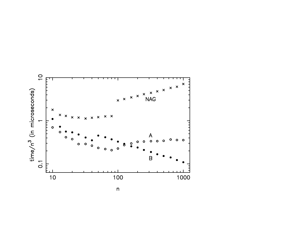
Fig. 7 shows the computing time (divided by for better clarity) as a function of , for three algorithms:
- •
Crosses correspond to the subroutine
H03ABFof the NAG library [10]. The time appears to grow asymptotically as . (A curious discontinuity is present: the computing time jumps up suddenly by a factor of about 2.2 between the values and . This is probably due to peculiarities of the computer hardware.) - •
Open circles represent Version A of the present algorithm (see Section 7.3). Computing time grows asymptotically as .
- •
Filled circles represent Version B of the present algorithm (see Section 7.3). For low values of , the computation is slower than with Version A because of the extra work involved in computing the distances . Above , however, this extra work begins to pay off. Computing time grows asymptotically as .
Version B is clearly the best method. For a problem, the NAG subroutine takes about 7000 seconds, while Version B takes about 110 seconds. The ratio increases for larger values of .
8.2 Degenerate case
A value was chosen as representative for a degenerate problem. In particular, this is a typical value for applications to lattice gas problems [5]. Thus, can take only integer values from 1 to 20.
Fig. 8 shows computing times as a function of , for two algorithms: the NAG subroutine and Version A of the present algorithm. (Version B is inefficient in the degenerate case and is not shown).
- •
For the NAG subroutine (crosses), computing time is essentially the same as in the non-degenerate case (Fig. 7) up to about . For larger values, the effect of the degeneracy begins to be felt and the slope decreases. Asymptotically, the computing time appears to grow as about .
- •
For the present algorithm (open circles), the decrease in computing time with respect to the non-degenerate case is more marked and starts earlier, at about . The time dependence is more complex. The final slope indicates a dependence in .
For a problem, the NAG subroutine takes 400 seconds, while Version A takes about 1.25 seconds. The ratio again increases for larger values of .

We remark that an exponent of less than 2 means that for large values of , the time needed to solve the problem is small compared to the time needed to set it up, since simply copying the matrix into memory takes a time proportional to ! Note also that in this situation, most values will never be used.
8.3 Assignment problem
Tests were also made for the particular case of the assignment problem, where and all rods have weights , . (It is then easily shown that an optimal solution obtained with the present algorithm automatically satisfies the constraint (10). In that case, comparisons can also be made with the subroutine LSAP of Burkard and Derigs [2] (noted BD here).
Fig. 9 compares computing times in the general (non-degenerate) case with . As before, the NAG subroutine is much slower. The BD algorithm is fastest: for a problem, computing time is about 45 seconds for Version B and 22 seconds for the BD algorithm. The difference decreases when increases, however: the asymptotic law is about for Version B, compared to for BD.
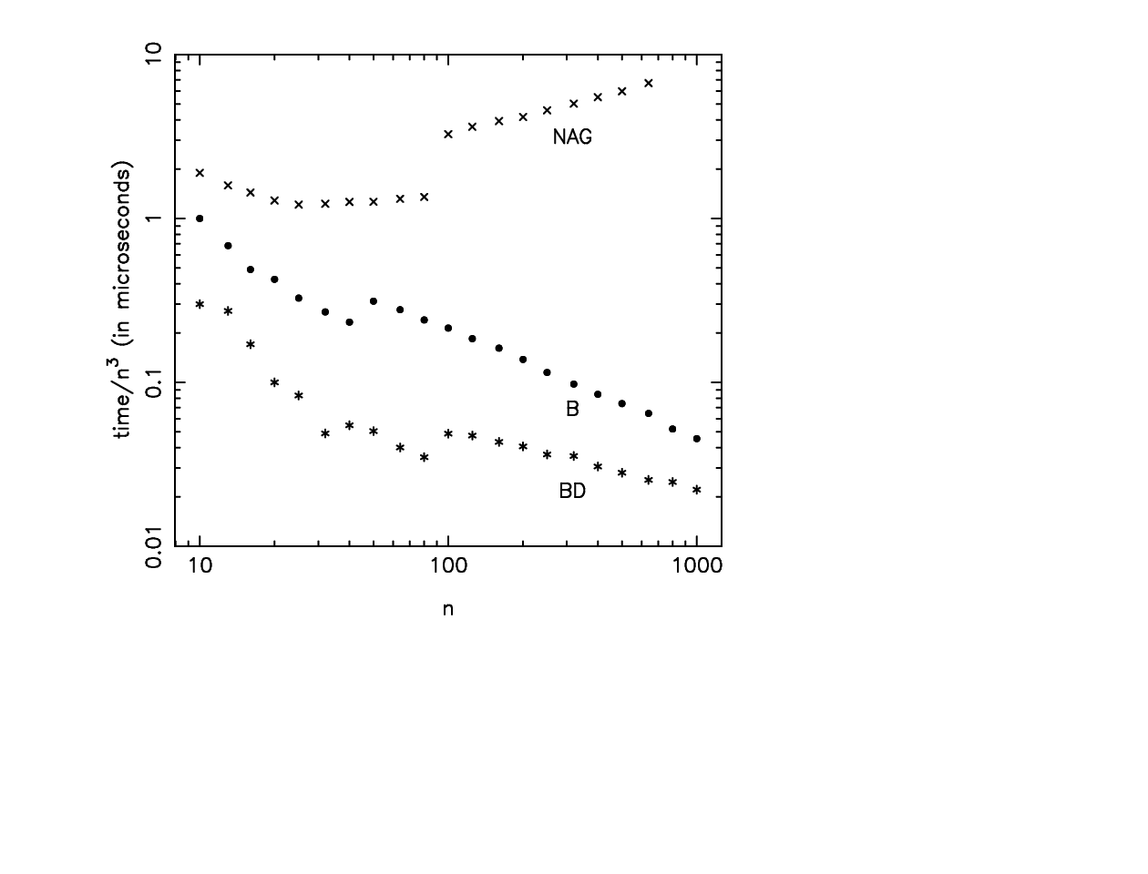
Fig. 10 compares NAG, Version A, and BD for the degenerate assignment problem, with . Here Version A is fastest: for a problem, computing time is 0.6 seconds for Version A, and 14 seconds for BD. The difference increases with : the asymptotic behaviour is in for Version A, for BD and NAG.

9 Final comments
1. Many variations of the present algorithm could be imagined, and it is quite possible that some of them would increase its speed. For instance, sometimes an arbitrary choice can be made for the contact edge or the breaking edge (see steps 3 and 5 in Section 6); one might try to determine what is the best choice.
2. As mentioned in the Introduction, the present algorithm was conceived and developed independently, without recourse to the existing litterature. Looking back, however, it becomes clear that some relations exist. The heights of the rods, for instance, are nothing else than the classical dual variables; hence the choice of the customary notations and in the present paper.
In particular, after this work was completed, M. Hartmann called our attention to the references [13] and [1]. These papers describe algorithms for the minimum cost flow problem, which includes the transportation problem as a special case. One starts from zero flow and continually increments it, maintaining at all times a minimum-cost solution, until the desired flow is attained. It appears that the algorithm of the present paper belongs essentially to the same family, known as parametric algorithms. The equivalent of the flow in the present model is the total force applied by the lines to the columns; as is easily shown, this total force starts from zero and increases with time, until it is equal to the total weight of the lines. More specifically, it increases by during each readjustment of the forces (Section 6.3, Step 4).
3. As mentioned in Section 7, most of the computing time in the present algorithm is spent on finding the minimum in a large set of numbers. Efficient algorithms have been developed for this operation on massively parallel computers [6]. A parallel implementation of the algorithm might therefore be of interest.
4. A comparison of figures 7 and 8, or 9 and 10, shows that the solution of the degenerate problem is much faster. This might be of interest in situations where a great accuracy is not required, or is not present in the data. In such cases, it will be very advantageous to round off the values so as to reduce them to a comparatively small set of values.
5. The idea of using mechanical analog computers for optimization problems is not new. For instance, reference [14] describes a mechanical device made of shafts and gears, which can in principle solve the general instance of the linear programming problem. However, this device is introduced in [14] only as a conceptual tool in a theoretical study of the complexity of analog computation; it is not intended as a model for a practical algorithm. We remark also that the mechanical model of the present paper is adapted to the special case of the transportation problem, and is therefore much simpler (and presumably more efficient) in that special case. As a rough measure, the present model has moving parts, while the model of [14] would have moving parts in a transportation problem.
In this connection, it is natural to ask whether the mechanical model used here to simulate the transportation problem can be extended to the more general minimum cost flow problem, or to the even more general linear programming problem. We have not found any obvious way to do this.
Appendix A Bounds on the maximal number of cycles
We call the maximal number of cycles, for the problem, using the algorithm described in Section 6. We derive here some rigorous bounds on this number.
A.1 Upper bound
We derive first a general upper bound for .
We number with an index the successive levels of the moving tree. The stop is at level , the sons of are at level , the grand-daughters of are at level , and so on. Note that odd levels correspond to rows and even levels to columns. We call the number of nodes of the tree at level . The sequence of numbers , , …, will be called the signature of the moving tree.
We consider now all possible signatures for given and , assuming that the final state has not yet been reached, i.e. that the moving tree still contains at least one row and the fixed tree still contains at least one column. We order these signatures as follows. First we sort by decreasing . Next we sort each subset by increasing . Next we sort each subsubset (corresponding to given and ) by decreasing ; and so on, always using decreasing order for odd values of and increasing order for even values. Finally, we number the sorted signatures with , 2, ….
It is then easy to show that always increases during a cycle. There are two cases:
- 1.
The moving tree captures a subtree from the fixed tree. The root of this subtree (after the capture) is a column. Therefore the first level at which there is a change in the signature is even, and increases by one unit. From the above sorting method it follows that increases.
- 2.
The moving tree loses a subtree. The root of this subtree (before the capture) is a row. Therefore the first level at which there is a change in the signature is odd, and decreases by one unit. Again increases.
Therefore we obtain an upper bound on the number of cycles simply by counting the signatures. We call the number of rows, and the number of columns in the moving tree. Since the moving tree is assumed to be non-empty, can take values from 1 to . Similarly, since the fixed tree is non-empty, can take values from 0 to . We evaluate first the number of signatures for given and . A signature can also be represented by a sequence of binary digits: we write digits 1, then digits 0, then digits 1, and so on. The first digit must be a 1. There are digits 0, which can be placed anywhere in the remaining positions. Therefore the number of possible signatures is
| (56) |
Summing over and , we obtain the following upper bound for :
| (57) |
Exactly the same considerations can be applied to the fixed tree. We number with the successive levels. We call the number of nodes at level . The sequence of numbers , , …, will be called the signature of the fixed tree. We sort the signatures, using decreasing order for odd (columns) and increasing order for even (rows). We number the sorted signatures with . The number also always increases during a cycle. We call the number of columns, and the number of rows in the fixed tree. Counting the number of signatures as above, we find
| (58) |
i.e. exactly the same upper bound as in (57).
A.2 Better upper bound
A much better upper bound can be obtained by noting that only some combinations of and are permitted. This is because we must have
| (59) |
Thus, in a plane, only a subset of points are allowed. Combining this with the fact that both and must increase at each step, one can trace the possible paths in the plane and derive an upper limit on the number of steps, which we call .
Unfortunately a general formula giving for arbitrary and has not been found. Results obtained by a computer program for values of and up to 10 are listed in Table 3.
|
||||||||||||||||||||||||||||||||||||||||||||||||||||||||||||||||||||||||||||||||||||||||||||||||||||||||||||||||||||||||||||||||||||||||||||||||||
For , for instance, we have , .
A.3 Lower bound
In the square case , the following lower bound can be proved:
| (60) |
The proof is cumbersome and will not be given here. It consists in showing that the number of cycles equals in the following case:
| (61) |
This was also verified by a direct application of the numerical algorithm for to 17. Note that the sequence , , , , …is the Fibonacci sequence, minus its first term.
A.4 Comparison with observed values
We observe that (62) corresponds to a computing time which grows exponentially with . Fortunately, numerical tests with randomly chosen examples show a much milder increase, which is approximately linear in . Table 4 compares the values (62) with the average observed values of the number of cycles, for Version B of the algorithm, in the non-degenerate case. The r.m.s. dispersions are also given; they show that individual values do not deviate much from the average.
|
This considerable difference between the “bad case” (61)and the average case can be probably understood by noting that (61) is a rather extreme case: the coefficients , , form essentially geometrical progressions. For , for instance, the ratio is of the order of . This is not likely to be encountered in applications.
A.5 Acknowledgements
I thank P. Bernhard, U. Frisch, M. Hartmann, J. Morgenstern, A. Noullez, K. Steiglitz, and S. Stidham for discussions and comments.
References
- [1] R. K. Ahuja, J. L. Batra, and S. K. Gupta, “A parametric algorithm for convex cost network flow and related problems,” European Journal of Operational Research 16 (1984) 222–235.
- [2] R. E. Burkard and U. Derigs, Assignment and Matching Problems: Solution Methods with FORTRAN-Programs, Lecture Notes in Economics and Mathematical Systems No. 184 (Springer, Berlin, 1980).
- [3] L. R. Ford and D. R. Fulkerson, Flows in Networks (Princeton University Press, 1962).
- [4] G. Hadley, Linear Programming (Addison-Wesley, Reading, Massachusetts, 1962).
- [5] M. Hénon, “Optimization of collision rules in the FCHC lattice gas, and addition of rest particles,” in: R. Monaco, ed., Discrete Kinetic Theory, Lattice Gas Dynamics and Foundations of Hydrodynamics, Proceedings of a Workshop held in Torino, September 20-24, 1988 (World Scientific, 1989) pp. 146–159.
- [6] W. D. Hillis and G. L. Steele, “Data Parallel Algorithms,” Communications of the Association for Computing Machinery 29 (1986) 1170–1183.
- [7] F. L. Hitchcock, “The distribution of a product from several sources to numerous localities,” Journal of Mathematical Physics 20 (1941) 224–230.
- [8] D. d’Humières, P. Lallemand, and U. Frisch, “Lattice gas models for 3D hydrodynamics,” Europhysics Letters 2 (1986) 291–297.
- [9] D. Knuth, The Art of Computer Programming, Volume 1 (Addison-Wesley, Reading, Massachusetts, 1973).
- [10] NAG Fortran Library, Mark 15 (NAG Ltd, Wilkinson House, Jordan Hill Road, Oxford, United Kingdom, 1991).
- [11] C. H. Papadimitriou and K. Steiglitz, Combinatorial Optimization: Algorithms and Complexity (Prentice-Hall, Englewood Cliffs, New Jersey, 1982).
- [12] J.-P. Rivet, M. Hénon, U. Frisch, and D. d’Humières, “Simulating fully three-dimensional external flow by lattice gas methods,” Europhysics Letters 7 (1988) 231–236.
- [13] S. R. Schmidt, P. A. Jensen, and J. W. Barnes, “An advanced dual incremental network algorithm,” Networks 12 (1982) 475–492.
- [14] A. Vergis, K. Steiglitz, and B. Dickinson, “The complexity of analog computation,” Mathematics and Computers in Simulation 28 (1986) 91–113.
Appendix B Addendum (September 2002)
The present paper was submitted to Mathematical Programming in May 1992. The following referee’s report was subsequently received:
(Beginning of referee’s report)
General comments
This well-written paper proposes an algorithm for the transportation problem that is motivated by an analog model, and has some comparisons of a code for this algorithm with a NAG code. The new algorithm is found to be much faster than the NAG code on randomly generated problems.
The author of this paper comes from outside the Math Programming community, and is to be commended for taking the time to bring his/her fresh perspective to the subject. However, it is tempting to dismiss this paper on the basis that the author has merely re-discovered a known algorithm, namely the one in [13], noting that [13] already contains a computational comparison of such an algorithm with other algorithms existing at the time. A further reasonable criticism of the current paper is that the NAG routine “H03ABF uses the ‘stepping stone’ method, modified to accept degenerate cases” (quoting from the NAG documentation), referenced in the book “Linear Programming” by G. Hadley, 1962 (this description should have been in the paper). The routine itself has been in the NAG library at least from 1975. Thus this code does not represent the current state of the art in transportation algorithms, as would be found, e.g., in Ahuja et al. Also, comparing codes on randomly generated problems can be misleading in any case.
On the other hand, I believe that in general such outside contributions should be valued, and specifically that this paper has something to offer if it is drastically re-written:
- 1.
The application of transportation problems to lattice gas models is intriguing, and is worth further discussion. Is there a short way to say how such models arise and the significance of the transportation subproblem? Also, do such problems tend to be sparse or dense, how big are and in typical problems, how large do the supplies and demands tend to be, and how large do the costs tend to be? These are all parameters that are important in assessing which of the standard modern algorithms might work well on such problems.
- 2.
The computational testing in the paper needs to be fixed. It would be more believable if the codes were tested on instances arising from the actual application rather than random problems. It would also be a service to the community to release several typical examples of such problems to, e.g., the DIMACS library of network flow instances, so that other codes can be tried on these problems. DIMACS also has available some well-tested random network generators; it enhances comparability between codes if standard generators are used instead of ad hoc generators. DIMACS codes and generators are available via anonymous ftp from dimacs.rutgers.edu in directory pub/netflow.
- 3.
I enjoyed the analog model and the physical insight it gives to the algorithm. In fact, I believe that a slightly different presentation of the algorithm that ties it more closely to the physical model would improve the paper: My suggestion is to make and into an extra row and column (which they effectively are in the model anyway), both with zero weight/buoyancy, and such that for all and . However, to act as stops in the initial configuration, we must give an artificial weight of , and an initial buoyancy of . The initial configuration is in fact optimal with these artificial weights. The aim of the algorithm is then to decrease the artificial weights to zero while maintaining optimality at each intermediate artificial weight value. Thinking of and as lines remove the need to treat them as special cases elsewhere.
- 4.
Much of the proof of the algorithm’s correctness is unnecessary since the author is just rediscovering well-known arguments, and has proposed an algorithm that fits nicely into known classes of algorithms. For example, equation (25) is known as complementary slackness, and the fact that complementary slackness plus feasibility equals optimality is so well-known that it can be stated without a reference. Although the author derived the algorithm independently of known algorithms, in order to effectively present it to an audience which is familiar with known algorithms it would be helpful to discuss the algorithm as if it were a special case of what is called “dual node-infeasible” simplex algorithms in [13]. I have in mind something like the following (assuming that suggestion 3 above is taken): The algorithm maintains dual feasible variables (the heights) and primal flows (forces; this correspondence between heights/forces and dual/primal variables is too important to leave it to a comment in the conclusion) that satisfy non-negativity and all supplies and demands except possibly at the extra nodes and , and ensures that the primal and dual variables satisfy complementary slackness. It also maintains a basic tree, namely the fixed tree plus the moving tree, plus the extra arc where fresh contact between the fixed and moving trees occurs. The extra arc allows some of the surplus supply at to be pushed through the tree to cancel out some of the surplus demand at . An arc whose flow drops to zero during this flow push can then be the dual simplex outarc, and a standard dual simplex pivot (whose two sides will be the fixed tree and the moving tree) will determine which is the new extra inarc to be added to the tree. This continues until there is no surplus supply or demand at or . This change would allow Section 6 to be reduced to a few sentences in Section 4, since it is well-understood that node-infeasible dual network simplex maintains dual feasibility, primal feasibility except for conservation, and complementary slackness, and that when conservation is achieved we must be optimal. Without this change and its attendant severe shortening, the paper is not publishable since large parts of it recapitulate familiar arguments.
- 5.
The Appendix should be shortened and moved into the text to establish what is known about how fast the algorithm converges. All that is needed is the observation that the algorithm is always finite without the need for any anti-degeneracy device (since signatures are lexicographically strictly increasing), that the upper bound is easy to derive, and that examples exist which use pivots. It should be pointed out that each piece of data in these examples has only bits, so the examples show that the algorithm is not even weakly polynomial. Also, either “iterations” or “pivots” is preferable to the word ”cycles”, since “cycles” is too suggestive of cycles in graphs.
- 6.
It seems possible that by using scaling (see, e.g., Ahuja et al.), a weakly polynomial version of the algorithm could be developed. The rough idea would be to scale the supplies and demands. Although in general this would lead to a problem where , the extra nodes would handily absorb the extra flow. When we optimize at one scale factor and want to move to the next one, supply or demand at a node might increase by one, and we need to regain optimality. I believe that we can do this by a shortest path computation at each such node, looking for the shortest distance path that will allow us to rehang the extra flow from the proper one of or . This can be done in polynomial time. We then have a problem where the total surplus supply/demand at and is . Degeneracy could cause a problem here since it makes it difficult to get a polynomial bound on iterations before optimality. I believe that the same shortest path trick can be used to ensure that each iteration moves at least one unit of flow. This shortest path business compresses several iterations into a single iteration, and might be useful in general. (Ideally, it would be nice to see a computational comparison of the shortest path version with the tree version of the algorithm on degenerate problems.) In addition, the shortest path neatly ties in with the notion of the reduced costs as “distances”, and is defensible in terms of the model as looking for the smallest distance to move the moving tree so that some of the force on and can be lessened. This form of the algorithm starts to look very much like the well-known successive shortest paths algorithm (see Ahuja et al.). In any case, a mention of a possible scaling version of the algorithm would be useful.
- 7.
Most readers will prefer the term “transportation problem” to “Hitchcock problem”.
References
- [1] Ahuja, R.K., T.L. Magnanti, and J.B. Orlin (1989). Network Flows. Chapter IV of Handbooks in Operations Research and Management Science, Volume 1: Optimization, eds. G.L. Nemhauser, A.H.G. Rinnooy Kan and M.J. Todd, North Holland, pp. 211-369.
(End of referee’s report)
Incidentally, I wish to thank here the unknown referee for taking the trouble to write such a detailed and helpful report.
It took me some time to obtain the necessary papers, to assimilate them and to re-do the calculations. In the end, I was able to convince myself that, unfortunately, the referee was entirely correct:
(i) The algorithm is not new. It is in fact identical, apart from some trivial changes, with the “parametric network simplex algorithm” described for instance in the book “Network flows”, published in 1993 by Ahuja, Magnanti and Orlin, pages 433–437.
(ii) The NAG algorithm which I used as a basis for comparison is not state of the art. I made comparisons with more modern algorithms, specifically with the results of Jianxiu Hao and George Kocur in the paper “An implementation of a shortest augmenting path algorithm for the assignment problem” (found on the Internet server dimacs.rutgers.edu, dated 1992), and my program does not show a marked advantage anymore.
Unfortunately I did not feel able to follow the suggestion of the referee and to drastically rewrite the paper; it would have been too much work, in a field with which I am not very familiar. So I published a much shorter version, including only the mechanical model (Section 3 of the present paper) in Comptes Rendus de l’Académie des Sciences, Paris, 321, Série I, 741–745 (1995).
Recently, some of my colleagues have used ideas from the present paper to solve a problem in cosmology (see “A reconstruction of the initial conditions of the Universe by optimal mass transportation”, by Uriel Frisch, Sabino Matarrese, Roya Mohayaee, Andrei Sobolevski, Nature, 417, 260–262 (2002) = astro-ph/0109483), and they asked me to make the paper generally available by submitting it to arXiv.
The present text is unchanged from the 1992 original, with two exceptions: a minor error has been corrected in Equ. (47), and the expression Hitchcock problem has been replaced by the more modern name transportation problem, as suggested by the referee.