Large $N$ dualities and transitions in geometryThanks: Research partially supported by the Institute for Advanced Study, and by National Science Foundation grants DMS-9706707, DMS-0074980, DMS-9729992 and by Italian MIUR’s grants. We thank the Institute for Advanced Study, the University of Pennsylvania and the Università di Torino for hospitality during various stages of this project.

A. Grassi and M. Rossi Address: Department of Mathematics, University of Pennsylvania, Philadelphia, PA 19104 Email address: grassi@math.upenn.edu Address: Dipartimento di Matematica, Università di Torino, via Carlo Alberto 10, 10123 Torino Email address: michele.rossi@unito.it

Abstract.

Survey article based on lectures given by the first author in May 2001 during 4th SIGRAV and SAGP2001 Graduate School.

The focus of these lectures is Gopakumar–Vafa’s insight that “Large $N$ dualities” (relating gauge theories and closed strings) are realized, in certain cases, by “transition in geometry”. In their pivotal 1998 example, the gauge theory is $SU(N)$ Chern-Simons theory on $S^{3}$ , for large $N$ , and the transition is the “conifold” transition between two Calabi–Yau varieties. Much progress has been made to support Gopakumar and Vafa’s conjecture, including the lift of the transition to a transformation between 7-manifolds with $G_{2}$ holonomy. In another direction, this set up leads us to consider the uncharted territory of “open Gromov-Witten invariants”. The lectures, hence the notes, were prepared for an audience of beginning graduate students, in mathematics and physics, whom we hope to get interested in this subject. Because most of the material presented in these lectures comes from the physics literature, we aimed to build a bridge for the mathematicians towards the physics papers on the subject.

In 1974 ’t Hooft conjectured that large $N$ gauge theories are dual to closed string theory. In 1998, Gopakumar and Vafa conjectured that $SU(N)$ Chern–Simons theory on $S^{3}$ is dual to II– $A$ string theory (with fluxes) compactified on a certain local Calabi–Yau manifold $Y$ , where the geometry of $Y$ is the key to the duality.

It is in fact possible to do a topological surgery on $Y$ (a birational contraction followed by a complex deformation in algebraic geometry) to obtain another Calabi–Yau $\widehat{Y}$ ; it turns out that $\widehat{Y}\cong T^{*}S^{3}$ . $Y$ and $\widehat{Y}$ are said to be related by a “geometric conifold transition”. By previous work of Witten, Chern–Simons theory on $S^{3}$ is equivalent to II– $A$ on $\widehat{Y}$ , with $SU(N)$ D-branes wrapped on $S^{3}$ .

Evidence for the conjecture comes by comparing the partition function for the Chern–Simons theory on $S^{3}$ and the partition function for II– $A$ on $Y$ . The corresponding mathematical quantities are certain topological invariants of $S^{3}$ and Gromov-Witten invariants on $Y$ ; knot invariants on $S^{3}$ and “open Gromov-Witten invariants” on $Y$ . The “open Gromov-Witten invariants” should “count” maps of Riemann surfaces with boundary to $Y$ . We use quotation marks, as they are not defined; yet, in this particular case (and, as it turns out many other cases) it is possible to make some working assumptions and compute invariants. There is still an ambiguity, but as it turns out there is also an ambiguity on the Chern–Simons side, and the ambiguities on both sides match.

The topic of the last lecture in Como was the strategy to prove the conjecture, proposed by Acharya, Atiyah, Maldacena and Vafa, by lifting the II– $A$ theories to $M-$ theory compactified on $7$ -dimensional manifolds with $G_{2}$ holonomy.

Section 3 contains the core of Gopakumar and Vafa’s conjecture and the work of ’t Hooft and Witten leading to it; we also present the evidence supporting the conjecture and its mathematical implications. In Section 4, we present the strategy of Acharya, Atiyah, Maldacena and Vafa and include some basics on spaces with $G_{2}$ holonomy.

The first Section describes in detail the geometry of the conifold transition between two manifolds (which are local Calabi–Yau), because the local geometry is the key to the duality. We also include two sections on transitions between Calabi-Yau threefolds and their significance in algebraic geometry and the physics of string theory. In Section 2 we present some background on Chern–Simons theory.

The lectures, hence the notes, were prepared for an audience of beginning graduate students, in mathematics and physics, whom we hoped to get interested in this subject. Because most of the material presented in these lectures comes from the physics literature, we aimed to build a bridge for the mathematicians towards the physics papers on the subject. On one hand, we tried to make these lectures self-contained and did not assume much knowledge beyond the first/second year courses. On the other, we thought it was important to outline links between these lectures and other research topics in string theory and mathematics, even when these were not essential to the main motif of the lectures. In these cases, we just gave statements, without necessarily defining all the terms involved.

We gloss over the notion of wrapped D-branes and Lagrangian submanifolds, as these were discussed in A. Lerda and K. Fukaya’s lectures, as well as many aspects of conformal field theory, the topic of Y. Stanev’s lectures. There is no discussion of II– $A$ theory itself, partly because of time constraints, partly because II– $A$ , II– $B$ theories and Gromov-Witten invariants have recently been in the spot light, thanks to the celebrated “mirror symmetry”.

Many of the results presented in these lectures appeared in preprint form, or were announced, while the lectures were prepared and given. Other related papers appeared afterwards; we do not discuss these papers, as the notes closely follow the lectures.

The second author attended the lectures and at the end wrote completely sections 2.3, 2.4 and the Appendices, which were only sketched in the lectures.

The first author would like to thank the organizers of the 4th SIGRAV Graduate School on contemporary relativity and gravitational physics and 2001 school on Algebraic Geometry and Physics (SAGP2001) for the opportunity to give these talks. We also would like to thank D. Freed, S. Katz, J. Maldacena and N. Seiberg for kindly explaining their work. Thanks are also due to B. Agboola, B. S. Acharya, R. Donagi, S. Garbiero, D. Harbater, P. Horja, K. Karu, D. Morrison, B. Ovrut, J. Talvacchia, K. Uhlenbeck, I. Zharkov and especially L. Traynor, for many useful conversations. We are very grateful to A. Greenspoon for his helpful comments on a previous draft.

A.G. is much indebted to D. E. Diaconescu, who patiently answered many questions on various topics concerning these lectures.

1. Geometry and topology of transitions

The focus of these lectures is Gopakumar-Vafa’s insight that “Large $N$ dualities” (relating gauge theories and closed strings) are realized, in certain cases, by “transition in geometry”. In their pivotal example [46] the gauge theory is $SU(N)$ Chern-Simons theory on $S^{3}$ , for large $N$ , and the transition is “the conifold transition” between two Calabi–Yau varieties $\widehat{Y}\supset S^{3}$ and $Y$ . Their conjecture is discussed in Section 3, while here we describe in detail the geometry of the conifold transition between two varieties. The local geometry is in fact the key to the duality.

We also include two sub-sections on transitions between Calabi-Yau threefolds and their significance in algebraic geometry and the physics of string theory.

$Y$ and $\widehat{Y}$ are local Calabi-Yau’s, i.e. open neighborhoods in Calabi-Yau manifolds. The Calabi-Yau condition is needed to preserve the supersymmetry of the physical (II– $A$ ) string theory:

Definition 1.1.

A Calabi--Yau manifold is a smooth $n$ –dimensional complex algebraic manifold with trivial canonical bundle, i.e. $\Omega_{Y}^{n}\cong\mathcal{O}_{Y}$ and such that

H^{j}\left(\mathcal{O}_{Y}\right)=0\ \ \forall j,\ \ \ 0<j<n.

It can be verified that hypersurfaces of degree $d+1$ in ${\mathbb{P}}^{d}$ are $(d-1)$ –Calabi-Yau manifolds. Elliptic curves and $K3$ surfaces are the $one$ and $two$ -dimensional Calabi-Yau manifolds.

This definition of Calabi-Yau variety is the most common in the algebraic geometry literature: it is the natural generalization of that of a $K3$ surface. It is worthwhile to keep in mind that there are other, non–equivalent, definitions of a Calabi-Yau threefold; we will discuss a definition, which is relevant in the physics context, and its equivalence to the following one in (4.3), Section 4. Note also that the current definition of $K3$ is different from the one originally used by Weil (see for example [14]). For a nice presentation of some of the different definitions and implications among them, see [62].

In the three–dimensional case it is first possible to have transitions between topologically different Calabi-Yau manifolds:

Definition 1.2.

([32], [75]) Let $Y$ be a Calabi-Yau threefold and $\phi:Y\longrightarrow\overline{Y}$ be a bimeromorphic contraction onto a normal variety. If there exists a complex deformation (smoothing) of $\overline{Y}$ to a smooth Calabi-Yau threefold $\widehat{Y}$ then the process from $Y$ to $\widehat{Y}$ is called a transition.

This concept plays an important role both in algebraic geometry and in superstring theory as we will see later. The following transition, the conifold transition, is the focus of the work of Vafa and collaborators and of these lectures; in 1.2 we briefly discuss other transitions of Calabi-Yau manifolds. This example is based on Clemens’ construction [30] and reported in [48] (see also [32], example 6.2.4.1).

Example 1.3.

(Conifold transition) Let $\overline{Y}\subset{\mathbb{P}}^{4}\left(x_{0}:\ldots:x_{4}\right)$ be the generic quintic threefold containing the plane $\pi$ defined by $x_{3}=x_{4}=0$ . It is the hypersurface defined by the equation

x_{3}g\left(x_{0},\ldots,x_{4}\right)+x_{4}h\left(x_{0},\ldots,x_{4}\right)=0

where $g,h$ are generic homogeneous polynomials of degree 4 (sections in $H^{0}\left(\mathcal{O}_{{\mathbb{P}}^{4}}\left(4\right)\right)$ ). $\overline{Y}$ is singular precisely at the sixteen points defined by the equations:

x_{3}=x_{4}=g=h=0.

We will see in 1.1 that the topology of the variety around each singular point is that of a real cone, hence the name conifold. The local equation defining each singularity is that of a node (see also Appendix 5 and equation (3) after the definition 1.4):

(1)

z_{1}z_{3}+z_{2}z_{4}=0\ \ \subset\mathbb{C}^{4}.

Now consider the threefold $Y\subset$ ${\mathbb{P}}^{4}\times{\mathbb{P}}^{1}$ defined by the equations:

(2)

\left\{\begin{array}[]{ll}y_{0}g\left(x_{0},\ldots,x_{4}\right)+y_{1}h\left(x_{0},\ldots,x_{4}\right)=0\\ y_{0}x_{4}-y_{1}x_{3}=0,\end{array}\right.

with $[y_{0},y_{1}]\in{\mathbb{P}}^{1}$ . It can be directly verified that $Y$ is smooth (or use Bertini’s theorem); then $\phi:Y\longrightarrow\overline{Y}$ is an isomorphism outside the sixteen nodes of $\overline{Y}$ and their inverse images in $Y$ , which are sixteen copies of ${\mathbb{P}}^{1}$ s. $Y$ is a birational resolution of $\overline{Y}$ (see Appendix 5); $\phi$ is also called a “small blow up” of $Y$ , because the inverse images of points are complex curves and not complex surfaces. In particular $K_{Y}\sim\phi^{*}(K_{\overline{Y}})\sim\mathcal{O}_{Y}$ , that is, $\phi$ is a crepant resolution (see 5). Moreover

h^{1,0}\left(Y\right)=h^{2,0}\left(Y\right)=h^{1,0}\left(\overline{Y}\right)=h^{2,0}\left(\overline{Y}\right)=0;

then $Y$ is a Calabi-Yau threefold with

h^{1,1}\left(Y\right)=h^{1,1}\left(\overline{Y}\right)+1=2.

Note also that all the contracted ${\mathbb{P}}^{1}$ ’s are on the same extremal ray of the Mori cone $\overline{NE}\left(Y\right),$ (see 5.4) i.e. $\phi$ cannot be factored in other contractions. $\phi$ is called a primitive contraction of type $I$ (see 1.2). On the other hand $\overline{Y}\subset{\mathbb{P}}^{4}$ can be deformed to the generic quintic threefold $\widehat{Y}\subset{\mathbb{P}}^{4}$ which is again a Calabi-Yau. The process of going from $Y$ to $\widehat{Y}$ is a (primitive) extremal transition of type $I$ . We will see in 1.1 that the topology of these singularities is that of a node: this transition is often called the conifold transition.

By Clemens’ topological analysis one can see that $Y$ and $\widehat{Y}$ do not have the same topology. See subsection 1.1 and theorem 1.6 for more details.

1.1. The local topology of a conifold transition

Here we analyze the local geometry and topology of a conifold transition $Y$ to $\widehat{Y}$ presented in example 1.3.

Definition 1.4.

A threefold singularity defined by the equation

x^{2}+y^{2}+z^{2}+v^{2}=0

is called a node (nodal singularity). (See Appendix 5.)

By a change of coordinates, the equation of the node can be rewritten as:

(3)

z_{1}z_{3}+z_{2}z_{4}=0,

via the affine transformation

(4)

\begin{array}[]{l}x=z_{1}+iz_{3}\\ y=z_{3}+iz_{1}\\ z=z_{2}+iz_{4}\\ v=z_{4}+iz_{2}.\end{array}

The singularities of example 1.3 are nodes.

Example 1.5.

The conifold, revisited.

The original threefold $\overline{Y}\subset{\mathbb{P}}^{4}$ is given by the equation:

x_{3}g\left(x_{0},\ldots,x_{4}\right)+x_{4}h\left(x_{0},\ldots,x_{4}\right)=0

By a linear projective transformation we may assume the point $P=\left(1:0:\ldots:0\right)$ to be one of the sixteen singular points of $\overline{Y}$ and localize our analysis in a neighborhood $\overline{U}$ of $P$ . By intersecting $\overline{Y}$ with the affine open subset of ${\mathbb{P}}^{4}$ defined by $x_{0}\neq 0$ we get the local equation of $\overline{U}\subset\mathbb{C}^{4}$

z_{3}\widetilde{g}\left(z_{1},\ldots,z_{4}\right)+z_{4}\widetilde{h}\left(z_{1},\ldots,z_{4}\right)=0

where $z_{i}:=x_{i}/x_{0}$ for $i=1,\ldots 4$ , $\widetilde{g}:=g/x_{0}^{4}$ and $\widetilde{h}:=h/x_{0}^{4}$ . Since $g$ and $h$ are generic we may assume $\widetilde{g}$ and $\widetilde{h}$ to be smooth maps $\mathbb{C}^{4}\longrightarrow\mathbb{C}$ submersive at the origin (i.e. at $P\in\overline{U}$ ) and by the inverse function theorem we have locally

	$\displaystyle\widetilde{g}\left(z_{1},\ldots,z_{4}\right)$	$\displaystyle=$	$\displaystyle z_{1}$
	$\displaystyle\widetilde{h}\left(z_{1},\ldots,z_{4}\right)$	$\displaystyle=$	$\displaystyle z_{2}$

up to a suitable analytic change of coordinates (this is the well known local submersion theorem).

Theorem 1.6.

([30], lemma 1.11)

(1)

Let $\overline{U}$ be the neighborhood of a threefold nodal singularity,
then $\overline{U}$ is a real cone over $S^{2}\times S^{3}$ .
(2)

Let ${U}$ be a neighborhood of the strict transform of a node in $Y$ , then
$U\cong D^{4}\times S^{2}\subset\mathbb{C}^{2}\times S^{2}.$
Furthermore $\mathcal{N}_{U|{\mathbb{P}}^{1}}\cong\mathcal{O}_{{\mathbb{P}}^{1}}\left(-1\right)\oplus\mathcal{O}_{{\mathbb{P}}^{1}}\left(-1\right)$ .
(3)

Let $\widehat{U}$ be the deformed neighborhood of a node, then
$\widehat{U}\cong D^{3}\times S^{3}\subset T^{*}S^{3}\cong\mathbb{R}^{3}\times S^{3}$ . In particular the non–trivial $S^{3}$ is the vanishing cycle of $\widehat{U}$ and it is locally embedded as a Lagrangian submanifold in $T^{*}S^{3}.$
(4)

The conifold transition is a local surgery which replaces a tubular neighborhood $D^{4}\times S^{2}$ of the exceptional fiber ${\mathbb{P}}_{\mathbb{C}}^{1}\cong S^{2}$ in $U$ by $S^{3}\times D^{3}$ to obtain a smoothing $\widehat{U}$ of $\overline{U}$ . In particular $U$ and $\widehat{U}$ are topologically different. This is the classical surgery between two manifolds with the same boundary.
(5)

More generally, there are relations between the Betti numbers of the Calabi–Yau manifolds $Y$ and $\widehat{Y}$ as in example 1.3.

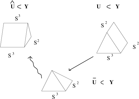
Refer to caption — Figure 1. The topology of the conifold transition

The invariants discussed in the rest of the paper are determined by the local geometry around the singular locus, so we identify (sometimes perhaps too freely) the Calabi-Yau manifolds $\widehat{Y}$ and $Y$ with the affine varieties $\mathbb{R}^{3}\times S^{3}$ and $\mathbb{R}^{4}\times S^{2}$ containing the local neighborhoods $\widehat{U}$ and $U$ .

The following proof of the theorem is a review of what is explained in the first section of [30] and also [25].

Proof:

(i) As we have seen in (3), the local equation of a threefold $\overline{U}$ with a nodal singularity at the origin is:

(5)

z_{1}z_{3}+z_{2}z_{4}=0,

Consider now the affine transformation

(6)

\begin{array}[]{l}w_{1}=\left(z_{1}+z_{3}\right)/2\\ w_{2}=i\left(-z_{1}+z_{3}\right)/2\\ w_{3}=\left(z_{2}+z_{4}\right)/2\\ w_{4}=i\left(-z_{2}+z_{4}\right)/2\end{array}

and set $w_{j}=u_{j}+iv_{j}$ ; we can now identify $\overline{U}$ with the subset $\overline{V}\subset\mathbb{R}^{8}$ defined by the equations:

(7)

\begin{array}[]{l}\sum_{j=1}^{4}u_{j}^{2}-\sum_{j=1}^{4}v_{j}^{2}=0\\ \sum_{j=1}^{4}u_{j}v_{j}=0.\end{array}

Note now that there is a diffeomorphism

\overline{V}\setminus\left\{\left(0,\ldots,0\right)\right\}\cong\left(\mathbb{R}^{4}\setminus\left\{\left(0,\ldots,0\right)\right\}\right)\times S^{2}

where $S^{2}$ is the unit sphere in $\mathbb{R}^{3}$ . In fact for every positive real number $\rho$ we can consider the radius $\rho$ hypersphere $S_{\rho}^{7}\subset$ $\mathbb{R}^{8}$ and the section $V_{\rho}:=S_{\rho}\cap\left(\overline{V}\setminus\left\{\left(0,\ldots,0\right)\right\}\right)$ . Clearly we get

\overline{V}\setminus\left\{\left(0,\ldots,0\right)\right\}=\coprod_{\rho\in\mathbb{R}_{>0}}V_{\rho}

On the other hand $V_{\rho}$ has equations

\begin{array}[]{l}\sum_{j=1}^{4}u_{j}^{2}=\sum_{j=1}^{4}v_{j}^{2}=\frac{\rho^{2}}{2}\\ \sum_{j=1}^{4}u_{j}v_{j}=0\end{array}

Hence $V_{\rho}\cong S^{3}\times S^{2}$ since the fiber over a fixed point $\left(u_{1}^{o},\ldots,u_{4}^{o}\right)\in S_{\rho/\sqrt{2}}^{3}$ is given by the subset of $\mathbb{R}^{4}\left(v_{1},\ldots,v_{4}\right)$ defined by

\begin{array}[]{l}\sum_{j=1}^{4}v_{j}^{2}=\frac{\rho^{2}}{2}\\ \sum_{j=1}^{4}u_{j}^{o}v_{j}=0\end{array}

which is clearly a $S^{2}$ . Therefore

(8)

\coprod_{\rho\in\mathbb{R}_{>0}}V_{\rho}\cong\left(\mathbb{R}_{>0}\times S^{3}\right)\times S^{2}\cong\left(\mathbb{R}^{4}\setminus\left\{\left(0,\ldots,0\right)\right\}\right)\times S^{2}

and $\overline{U}\cong\overline{V}$ identifies with the real cone over $S^{3}\times S^{2}$ .

$\bullet$ (ii) The blown up conifold, the small resolution of a nodal singularity.

Motivated by formula (2), we consider the standard projection
$\phi:\mathbb{C}^{4}\times{\mathbb{P}}^{1}\to\mathbb{C}^{4}$ and its restriction to the open smooth threefold $U\subset\mathbb{C}^{4}\times{\mathbb{P}}^{1}$ defined by:

(9)

\begin{array}[]{l}y_{0}z_{4}-y_{1}z_{3}=0\\ y_{0}z_{1}+y_{1}z_{2}=0,\end{array}

with $[y_{0},y_{1}]\in{\mathbb{P}}^{1}$ . $\phi_{|U}=\varphi:U\longrightarrow\overline{U}$ . Recall that $\overline{U}$ is defined by the equation $z_{1}z_{3}+z_{2}z_{4}=0$ and has a nodal threefold singularity at the origin. $\varphi$ induces an isomorphism between the open sets $U\setminus\phi^{-1}\left(P\right)\cong\overline{U}\setminus\left\{\left(0,\ldots,0\right)\right\}\cong\overline{V}\setminus\left\{\left(0,\ldots,0\right)\right\}$ . As in the previous, compact example, $U\to\overline{U}$ is a birational resolution of $\overline{U}$ (see Appendix 5).

This “small resolution” of $\overline{U}$ was obtained by “blowing up” the plane $z_{3}=z_{4}=0$ ; by blowing up the plane $z_{3}=z_{2}=0$ we would have another small resolution $U_{+}$ isomorphic to $U$ outside the locus of the exceptional curves. $U_{+}$ is called the flop of $U$ and the birational transformation

(10)

U\leftarrow\cdots\rightarrow U_{+}

the “flop”. By analogy the transformation in Section 4 will also be called a flop.

In particular we then have a diffeomorphism

(11)

U\setminus\phi^{-1}\left(P\right)\cong\left(\mathbb{R}^{4}\setminus\left\{\left(0,\ldots,0\right)\right\}\right)\times S^{2}

and we want to extend it to the exceptional fiber $\phi^{-1}\left(P\right)\cong{\mathbb{P}}^{1}\cong S^{2}$ to give a diffeomorphism

(12)

U\cong\mathbb{R}^{4}\times S^{2}

In order to construct it observe that under the affine transformation $\left(\text{\ref{affinity}}\right)$ and the above identification $\mathbb{C}^{4}\left(w_{1},\ldots,w_{4}\right)\cong\mathbb{R}^{8}\left(u_{1},\ldots,u_{4},v_{1},\ldots,v_{4}\right)$ the neighborhood $U$ is sent diffeomorphically onto the subset of $\mathbb{R}^{8}\times{{\mathbb{P}}_{\mathbb{C}}}^{1}$ defined by

(13)

\begin{array}[]{l}y_{0}u_{3}+y_{0}v_{4}-y_{1}u_{1}-y_{1}v_{2}+i\left(y_{0}v_{3}-y_{0}u_{4}-y_{1}v_{1}+y_{1}u_{2}\right)=0\\ y_{0}u_{1}-y_{0}v_{2}+y_{1}u_{3}-y_{1}v_{4}+i\left(y_{0}v_{1}+y_{0}u_{2}+y_{1}v_{3}+y_{1}u_{4}\right)=0\end{array}

Hence the fiber over a fixed point $\left(y_{0}:y_{1}\right)^{o}\in{\mathbb{P}}_{\mathbb{C}}^{1}$ is a $\mathbb{R}^{4}\subset\mathbb{R}^{8}$ ensuring the existence of the diffeomorphism $\left(\text{\ref{local-blow}}\right)$ up to possibly shrinking $U$ . Moreover by splitting $y_{0}$ and $y_{1}$ into real and imaginary parts the equations $\left(\text{\ref{eqs}}\right)$ reduce to the following matricial form:

\mathbf{v}=A\mathbf{u}

where $\mathbf{u}$ and $\mathbf{v}$ are vectors whose entries are given by $u_{j}$ and $v_{j}$ respectively and $A$ is an antisymmetric matrix uniquely determined by the fixed projective point $\left(y_{0}:y_{1}\right)^{o}$ . Since outside of the origin the coordinates $u_{j}$ and $v_{j}$ have to satisfy the equations $\left(\text{\ref{real-node}}\right)$ this suffices to show that the restriction of the diffeomorphism $\left(\text{\ref{local-blow}}\right)$ to $U\setminus\phi^{-1}\left(P\right)$ gives precisely the diffeomorphism $\left(\text{\ref{punctured blow}}\right)$ .

Note that $U$ can be identified with the total space of the normal bundle $\mathcal{N}_{U|{\mathbb{P}}^{1}}$ , which is a holomorphic vector bundle of rank 2 over ${\mathbb{P}}^{1}$ . By the Grothendieck theorem (see for instance [78]) we have the splitting

\mathcal{N}_{U|{\mathbb{P}}^{1}}\cong\mathcal{O}_{{\mathbb{P}}^{1}}\left(d_{1}\right)\oplus\mathcal{O}_{{\mathbb{P}}^{1}}\left(d_{2}\right)

for some $d_{1},d_{2}\in\mathbb{Z}$ . The local equations $\left(\text{\ref{blow-node}}\right)$ allows us to determine those integers. In fact we can choose two local charts on $S^{2}\cong{\mathbb{P}}^{1}\left(y_{0}:y_{1}\right)$ around the north and the south poles respectively. Say $\tau:=y_{0}/y_{1}$ and $\sigma:=y_{1}/y_{0}$ are the two local coordinates on ${\mathbb{P}}^{1}$ . Lifting these charts to $\mathcal{N}_{U|{\mathbb{P}}^{1}}$ we can choose the two local parameterizations

\left(\tau,z_{1}\right)\oplus\left(\tau,z_{4}\right)\quad,\quad\left(\sigma,-z_{2}\right)\oplus\left(\sigma,z_{3}\right).

Look at the fibre over a fixed point $\left(y_{0}:y_{1}\right)=\left(\tau:1\right)=\left(1:\sigma\right)$ in the gluing of the charts. Since here $\sigma=\tau^{-1}$ by the local equations $\left(\text{\ref{blow-node}}\right)$ we get

	$\displaystyle-z_{2}$	$\displaystyle=$	$\displaystyle\sigma^{-1}z_{1}=\tau z_{1}$
	$\displaystyle z_{3}$	$\displaystyle=$	$\displaystyle\sigma^{-1}z_{4}=\tau z_{4}$

which means that the transition functions $\tau^{-d_{1}},\tau^{-d_{2}}\in\mathbb{C}^{*}=GL\left(1,\mathbb{C}\right)$ are given by $\tau$ , i.e. $d_{1}=d_{2}=-1$ .

(iii) The deformed conifold as a symplectic manifold.

Consider the (real) 1–parameter family of local smoothings $\widehat{U}_{t}$ of $\overline{U}$ defined by

(14)

\begin{array}[]{l}\sum_{j=1}^{4}u_{j}^{2}-\sum_{j=1}^{4}v_{j}^{2}=t\\ \sum_{j=1}^{4}u_{j}v_{j}=0\end{array}\ ,\ t\in\mathbb{R}_{>0}

Note that the generic quintic hypersurface $\widehat{Y}\subset{\mathbb{P}}^{4}$ smoothing $\overline{Y}$ in the example 1.3 can be chosen to admit local equations as in $\left(\text{\ref{smoothing}}\right)$ for some real $t_{o}>0$ since the real 1–dimensional arc parametrized by $t$ can be chosen transversely with respect to the Zariski closed subset of singular quintic hypersurfaces and connecting $\overline{Y}$ to $\widehat{Y}$ . Consider now the map

\mathbb{R}^{8}\left(u_{1},\ldots,u_{4},v_{1},\ldots,v_{4}\right)\longrightarrow\mathbb{R}^{8}\left(q_{1},\ldots,q_{4},p_{1},\ldots,p_{4}\right)

defined by setting

(15)

\begin{array}[]{l}q_{j}=\frac{u_{j}}{\sqrt{t+\sum_{i}v_{i}^{2}}}\\ p_{j}=v_{j}\end{array}

For every $t>0$ it maps $\widehat{U}_{t}$ diffeomorphically onto the cotangent bundle $T^{*}S^{3}\cong S^{3}\times\mathbb{R}^{3}$ to the unit sphere $S^{3}\subset\mathbb{R}^{4}\left(q_{1},\ldots,q_{4}\right)$ embedded in $\mathbb{R}^{8}$ as follows:

(16)

\begin{array}[]{l}\sum_{j=1}^{4}q_{j}^{2}=1\\ \sum_{j=1}^{4}q_{j}p_{j}=0\end{array}

Note that the 3–cycle $S_{t}\subset\widehat{U}_{t}$ described in $\mathbb{R}^{8}$ by

\begin{array}[]{l}\sum_{j=1}^{4}u_{j}^{2}=t\\ v_{1}=\ldots=v_{4}=0\end{array}

which vanishes when $t=0$ , is diffeomorphically sent onto the unit sphere $S^{3}\subset T^{*}S^{3}$ .

The canonical symplectic form given by

\omega:=d\vartheta

where $\vartheta:=\sum_{j=1}^{4}p_{j}dq_{j}$ is the Liouville form of $\mathbb{R}^{8}$ , induces a vanishing symplectic form on $S^{3}$ since this sphere is described in $T^{*}S^{3}$ by $p_{1}=\ldots=p_{4}=0$ (locally only three of these equations are needed). This shows that $S^{3}$ is a Lagrangian subvariety of $T^{*}S^{3}$ :

Definition 1.7.

A subvariety $Y\subset X$ is called Lagrangian if $\dim Y=\left(1/2\right)\dim X$ and the symplectic form $\omega$ of $X$ vanishes on every tangent vector to $Y$ i.e.

\forall p\in Y,\ \forall u,v\in T_{p}Y\quad\omega\left(u,v\right)=0

The same is then true for the vanishing cycle $S_{t}\subset\widehat{U}_{t}$ .

$\bullet$ (iv) The local description of the conifold transition. Consider the diffeomorphism:

(17)

\alpha:(\mathbb{R}^{4}(\mathbf{u})\setminus\mathbf{0})\times\mathbb{R}^{4}(\mathbf{v})\longrightarrow(\mathbb{R}^{4}(\mathbf{q})\setminus{\ \mathbf{0}})\times\mathbb{R}^{4}(\mathbf{p})

given by

\begin{array}[]{l}q_{j}=\frac{u_{j}}{\sqrt{\sum_{i}u_{i}^{2}}}\\ p_{j}=v_{j}\sqrt{\sum_{i}u_{i}^{2}}.\end{array}

Note that, by $\left(\text{\ref{real-node}}\right)$ and $\left(\text{\ref{ctg-bundle}}\right)$ , $\alpha$ restricts to a diffeomorphism

(18)

U\setminus\phi^{-1}\left(P\right)\cong\left(\mathbb{R}^{4}\setminus\left\{\mathbf{0}\right\}\right)\times S^{2}\stackrel{{\scriptstyle\alpha}}{{\cong}}S^{3}\times\left(\mathbb{R}^{3}\setminus\left\{\mathbf{0}\right\}\right)

In particular the fiber over a fixed point $\mathbf{u}^{o}\in\mathbb{R}^{4}\setminus\left\{\mathbf{0}\right\}$ such that $\sum_{i}\left(u_{i}^{o}\right)^{2}=\rho^{2}$ , which is the 2–sphere $S_{\rho}^{2}\subset$ $\mathbb{R}^{4}\left(\mathbf{v}\right)$ given by $\sum_{j}v_{j}^{2}-\rho^{2}=\sum_{j=1}^{4}u_{j}^{o}v_{j}=0$ , is diffeomorphically sent onto the fiber over the fixed point $\mathbf{q}^{o}=\alpha\left(\mathbf{u}^{o}\right)$ , which is the 2–sphere $S_{\rho^{2}}^{2}\subset$ $\mathbb{R}^{4}\left(\mathbf{p}\right)$ given by $\sum_{j}p_{j}^{2}-\rho^{4}=\sum_{j=1}^{4}q_{j}^{o}p_{j}=0$ . Calling $D^{n}$ the closed unit ball in $\mathbb{R}^{n}$ , this means that $\alpha$ restricts to give a diffeomorphism

(19)

\left(D^{4}\setminus\left\{\mathbf{0}\right\}\right)\times S^{2}\stackrel{{\scriptstyle\alpha}}{{\cong}}S^{3}\times\left(D^{3}\setminus\left\{\mathbf{0}\right\}\right)

which reduces to the identity on their boundaries $S^{3}\times S^{2}$ . Hence recalling $\left(\text{\ref{local-blow}}\right)$ we can cut out the interior of a $D^{4}\times S^{2}$ around the exceptional fibre $\phi^{-1}\left(P\right)$ in $U$ and paste in by $\alpha$ the interior of a $S^{3}\times D^{3}$ to get $\widehat{U}_{t}$ for some $t>0$ .

$\bullet$ (v) The Betti numbers.

If $\overline{Y}$ has $N$ nodes (and no other singular points) and $\delta$ is the number of linearly independent vanishing cycles in the smoothing $\widehat{Y}$ , we get the following relationship between the Betti and the Euler numbers of $Y$ and $\widehat{Y}$ :

(20)

\begin{array}[]{l}b^{3}\left(Y\right)=b^{3}\left(\widehat{Y}\right)-2\delta\\ b^{2}\left(Y\right)+b^{4}\left(Y\right)=b^{2}\left(\widehat{Y}\right)+b^{4}\left(\widehat{Y}\right)+2\left(N-\delta\right)\\ \chi\left(Y\right)=\chi\left(\widehat{Y}\right)+2N\end{array}

(see [30] and [107] for detailed proofs). Note that by the Calabi-Yau condition the first equation above gives the following relationship between the Hodge numbers of $Y$ and $\widehat{Y}$ :

h^{2,1}\left(Y\right)=h^{1,2}\left(Y\right)=h^{2,1}\left(\widehat{Y}\right)-\delta=h^{1,2}\left(\widehat{Y}\right)-\delta.\ \ \diamondsuit

The invariants discussed in the rest of the paper are determined by the local geometry around the conifold locus, so we identify the local Calabi-Yau’s $Y,\ \widehat{Y}$ and $\overline{Y}$ with the local neighborhoods $U,\ \widehat{U}$ and $\overline{U}$ .

1.2. Transitions of Calabi-Yau threefolds

Let $Y$ and $\overline{Y}$ be projective Calabi-Yau manifolds and $\phi$ a birational contraction. See Appendix 5 for the definitions of the different types of singularities used in this section.

Definition 1.8.

$\phi:Y\to\overline{Y}$ is a primitive contraction if it cannot be further factored into birational morphisms of normal varieties.

A non–primitive Calabi-Yau contraction may be factored into a composite of primitive contractions (see [108]), so, without loss of generality we can consider $\phi$ to be primitive. In this case the pull–back $\phi^{*}H$ of an ample divisor $H$ on $\overline{Y}$ will cut the Mori cone (see 5.4) $\overline{NE}\left(Y\right)$ along an extremal face. Such contractions are also called extremal and the associated transitions primitive extremal transitions.

Definition 1.9.

[109] A primitive contraction is:

•

of type $I$ if the exceptional locus $E$ of the associated primitive contraction $\phi$ is composed of finitely many curves,
•

of type $II$ if $\phi$ contracts a divisor down to a point,
•

of type $III$ if $\phi$ contracts a divisor down to a curve.

In the first case $\phi\left(E\right)$ is composed of a finite number of isolated singularities, each with a small resolution. Since $Y$ is smooth these singularities are necessarily terminal of index 1 and therefore cDV points. In the second case $E$ must be irreducible and more precisely it is a del Pezzo surface (see [86]); $\phi\left(E\right)$ is a canonical singular point of index 1.

In the third case $E$ is again an irreducible surface contracted down to a curve $\phi\left(E\right)$ of canonical singularities for $\overline{Y}$ . In particular if $\phi$ is crepant then $E$ is a conic bundle over the curve $\phi\left(E\right)$ which is a smooth curve of (generically $cA_{1}$ or $cA_{2}$ ) cDV points (see [86] and [109], theorem 2.2).

The simplest example of a non–trivial transition of type $I$ is the conifold transition of example 1.3, i.e. a transition allowing only isolated simple double points (nodes) for $\overline{Y}$ . In fact these singularities can (at least locally) be smoothed. The following results also hold:

Theorem 1.10.

(Friedman [40]) If $\phi$ is of type $I$ and the singularity is an ordinary double point, then $\overline{Y}$ is smoothable unless $\phi$ is the contraction of a single ${\mathbb{P}}^{1}$ to an ordinary double point.

Theorem 1.11.

(Altmann, Gross, Schlessinger) ([4, 51, 52, 91]

•

If $\phi$ is of type $II$ and $\overline{Y}$ is $\mathbb{Q}$ –factorial, then $\overline{Y}$ is smoothable unless $E\cong{\mathbb{P}}^{2}$ or $E\cong\mathbb{F}_{1}$
•

If $\phi$ is of type $III$ and $\overline{Y}$ is $\mathbb{Q}$ –factorial, then $\overline{Y}$ is smoothable unless $\phi(E)\cong{\mathbb{P}}^{1}$ and $E^{3}={7},\ {8}$ .

After Clemens’ work (see 1.1), Reid suggested that the birational classes of Calabi-Yau threefolds would fit together into one irreducible family (see [89]). In fact he speculated that transitions may connect a general Calabi-Yau threefold to a non–Kähler analytic threefold with trivial canonical class, Betti number $b_{2}=0$ and diffeomorphic to a connected sum of $N$ copies of $S^{3}\times S^{3}$ , where $N$ is arbitrarily large. This conjecture is usually known as Reid’s fantasy. There exist various pieces of evidence for this conjecture (the Calabi-Yau web: see e.g. [12], [29]).

1.3. Transitions and mirror symmetry

Assume that there exists a transition from $Y_{1}$ to $\widehat{Y}_{1}$ , factorizing through a birational contraction $\phi:Y_{1}\longrightarrow\overline{Y}_{1}$ ; assume also that the mirror partners ${Y}_{2}$ of $Y_{1}$ and $\widehat{Y}_{2}$ of $\widehat{Y}_{1}$ exist (see, for example, [75]).

It is believed that the mirror partners $\widehat{Y}_{2}$ and ${Y}_{2}$ are also connected by a transition, which factorizes through a birational contraction $\phi^{\circ}:\widehat{Y}_{2}\longrightarrow\overline{Y}_{2}$ ; the transition between $\widehat{Y}_{2}$ and ${Y}_{2}$ is often called the ‘‘reverse transition”. It is not known if this conjecture holds; see for example [15], for the case of the conifold transition.

The mirror symmetry exchanges the Hodge numbers $h^{1,2}$ (representing the dimension of the complex moduli space) with $h^{1,1}$ (the Kähler moduli space) of the Calabi-Yau mirror partners; this exchange is consistent with a partner mirror transition as we have seen in subsection 1.1. [49] outlined an heuristic approach to “continuously” extending mirror symmetry to all the Calabi-Yau threefolds belonging to the same connected component of the web generated by conifold transitions. Actually if transitions would connect to each other all Calabi-Yau threefolds, which is a rough version of Reid’s fantasy, then it could give an approach to establish mirror symmetry for all of them.

In the examples studied by [27] and [75] $Y_{1}$ , ${\widehat{Y}}_{1}$ and their mirrors are related by a primitive contraction of type $III$ (see Appendix 6).

1.4. Transitions, black holes etc.

The transitions among Calabi–Yau manifolds are crucial also in the context of string theory, as they connect two topologically distinct compactifications of a 10–dimensional type II string theory (to 4–dimensional string vacua). Since, in spite of the small number of consistent 10–dimensional string theories, their Calabi-Yau compactifications give rise to a multitude of 4–dimensional topologically distinct string vacua, transitions may result to be the suitable mathematical tool which is able to restore a concept of uniqueness in compactified string theory when mirror symmetry and a version of Reid’s fantasy (the Calabi-Yau web) is assumed. The physical interpretation would then be that two 4–dimensional topologically distinct string vacua may be connected to each other by means of a black hole condensation. This is the work of [48], [98].

Strominger gave a physical explanation of how to resolve the conifold singularities of the moduli space of classical string vacua by means of massless Ramond--Ramond (RR) black holes (see Appendix 7).

In [48] the transformation of a massive black hole into a massless one at the conifold model is called condensation. Not only conifold transitions have a physical counterpart. For example a similar interpretation involves transitions of type $II$ in the context of string–string duality (see [64], [16], [17]).

Transitions of Calabi–Yau manifolds also have a role in 5–dimensional supersymmetric theories (see for example [76], [36]).

2. Chern–Simons theory

We discuss some basics of classical Chern-Simons theory (following [28] and[38]) and of its quantum version (following [110] and [66]).

The first evidence for the conjecture comes from comparing the expansion of the Chern-Simons partition function (with and without knots), so the last section is dedicated to the computational aspects and link invariants. We start with a quick review of the mathematical background for Chern–Simons theory, principal bundles and connections: Appendix 8 contains more details.

Let $\pi:P\rightarrow M$ be a principal $G$ -bundle with $G$ acting on the right (see definition 8.1). In particular, for any $m\in M$ , $\pi^{-1}(m)\cong G$ . The differential of this map gives an isomorphism between the tangent space $\pi^{-1}(m)$ to each fiber at a point $p\in\pi^{-1}(m)$ :

d\pi:T_{p}\pi^{-1}\left(m\right)\stackrel{{\scriptstyle\cong}}{{\longrightarrow}}T_{id}G\cong\mathfrak{g}

Let $TP$ denote the tangent bundle of $P$ :

Definition 2.1.

The vertical bundle on $P$ is the vector sub–bundle $\mathcal{V}P$ of $TP$ given by $\ker\left(d\pi\right)$ ; that is, for every $p\in P$

\mathcal{V}_{p}P:=\ker\left[d_{p}\pi:T_{p}P\longrightarrow T_{\pi\left(p\right)}M\right]

Then the vertical bundle $\mathcal{V}P$ associated with the principal $G$ –bundle $\left(P,\pi\right)$ is a vector bundle whose standard fibre is the Lie algebra $\mathfrak{g}$ associated with $G$ (see remark 8.4).

A connection is an infinitesimal version of a $G$ -equivariant family of sections of $\pi:P\to M$ .

Definition 2.2.

A connection on a principal $G$ –bundle $\left(P,\pi\right)$ is a vector sub-bundle $\mathcal{H}P$ of $TP$ such that

(21)

TP=\mathcal{H}P\oplus\mathcal{V}P

and for every $p\in P$ and $\sigma\in G$

(22)

d_{p}R\left(\sigma\right)\left(\mathcal{H}_{p}P\right)=\mathcal{H}_{p\sigma}P

where $R$ is the right action of $G$ on $P$ (see definition 8.1).

Definition 2.3.

(1)

The connection form of a connection $\mathcal{H}P$ is the $\mathfrak{g}$ –valued 1–form $A\in\Omega^{1}\left(P,\mathfrak{g}\right)$ such that, for every $p\in P$ and $u\in T_{p}P$

(23) $A_{p}u:=\left(d_{id}\lambda_{p}\right)^{-1}\left(\mathcal{V}_{p}u\right)\in T_{id}G\cong\mathfrak{g}$

where $\lambda_{p}:G\stackrel{{\scriptstyle\cong}}{{\longrightarrow}}\pi^{-1}\left(\pi\left(p\right)\right)\subset P$ is the diffeomorphism given by $\lambda_{p}\left(\sigma\right):=p\sigma$ . It is a characteristic form of the connection $\mathcal{H}P$ since $\mathcal{H}P=\ker A$ (see proposition 8.6).
(2)

The curvature form of a connection $\mathcal{H}P$ is the $\mathfrak{g}$ –valued 2–form $\Omega\in\Omega^{2}\left(P,\mathfrak{g}\right)$ defined by:

(24) $\Omega_{p}\left(u,v\right):=-A_{p}\left[U,V\right]_{p},\ \ \ \forall p\in P,\ u,v\in T_{p}P$

where $U,V$ are any horizontal vector fields on $P$ extending the horizontal parts $\mathcal{H}_{p}u$ and $\mathcal{H}_{p}v$ of $u$ and $v$ respectively (recall the splitting $\left(\text{\ref{split}}\right)$ ).

Definition 2.4.

A gauge transformation of $P$ is an automorphism $\varphi$ of $P$ which induces the identity map on the base manifold $M$ .

Gauge transformations on $P$ form a group $\mathcal{G}_{P}$ , and $\left(\text{\ref{gauge on connection}}\right)$ defines an action of $\mathcal{G}_{P}$ on the affine space of connections $\mathcal{A}_{P}$ (see proposition 8.6).

Definition 2.5.

Let $\gamma:I:=\left[0,1\right]\longrightarrow M$ be a loop with base point $m\in M$ and let $\widetilde{\gamma}_{p}:I\longrightarrow P$ be the unique horizontal lift of $\gamma$ with initial point $p\in P$ , i.e. such that

d\widetilde{\gamma}_{p}\left(TI\right)\subset\mathcal{H}P\text{\quad and}\quad\widetilde{\gamma}_{p}\left(0\right)=p

Define a diffeomorphism of the fibre $\pi^{-1}\left(m\right)$ by

(25)

\begin{array}[]{cccc}h_{\gamma}:&\pi^{-1}\left(m\right)&\longrightarrow&\pi^{-1}\left(m\right)\\ &p&\longmapsto&\widetilde{\gamma}_{p}\left(1\right)\end{array}

Then:

(26)

\text{Hol}_{\mathcal{H}P}\left(m\right):=\{h_{\gamma}:\gamma\text{ is a loop based at }m\}

is a group (with the composition of morphisms), called the holonomy group of the connection $\mathcal{H}$ $P$ at $m\in M$ .

If the base manifold $M$ is connected all these groups are isomorphic by $\left(\text{\ref{connect-hol}}\right)$ . Then Hol_HP is called the holonomy group of the connection $\mathcal{H}$ $P$ .

Note that for every $p\in P$ it is possible to identify Hol ${}_{\mathcal{H}P}\left(\pi\left(p\right)\right)$ with the subgroup of $G$

(27)

G_{\mathcal{H}P}\left(p\right):=\left\{\sigma_{\gamma}\left(p\right)\in G:h_{\gamma}\left(p\right)=p\sigma_{\gamma}\left(p\right)\text{ and }h_{\gamma}\in\text{Hol}_{\mathcal{H}P}\left(\pi\left(p\right)\right)\right\}

If $p,q\in\pi^{-1}\left(m\right)$ then $G_{\mathcal{H}P}\left(p\right)$ and $G_{\mathcal{H}P}\left(q\right)$ are conjugate subgroups and they coincide if $p$ and $q$ can be joined by a horizontal curve in $P$ .

Definition 2.6.

The restricted holonomy group of the connection $\mathcal{H}$ $P$ at $m\in M$

(28)

H_{\mathcal{H}P}^{\left(o\right)}\left(m\right)\subset\text{Hol}_{\mathcal{H}P}\left(m\right)

is defined by considering homotopically trivial loops based at $m$ .

As before, if $M$ is connected we can define the restricted holonomy group $H_{\mathcal{H}P}^{\left(o\right)}\subset\$ Hol_HP. Moreover for every $p\in P$ we can identify the restricted holonomy subgroup $H_{\mathcal{H}P}^{\left(o\right)}\left(\pi\left(p\right)\right)$ with a suitable subgroup $G_{\mathcal{H}P}^{\left(o\right)}\left(p\right)\subset G_{\mathcal{H}P}\left(p\right)\subset G$ .

2.1. Classical Chern–Simons action

Let us assume the base manifold $M=\pi\left(P\right)$ to be a smooth and compact 3–manifold. Let $\mathcal{A}_{P}$ be the affine space of all possible connections on $P$ and choose $A\in\mathcal{A}_{P}$ with associated connection $\mathcal{H}P=\ker A$ . If $\Omega\in\Omega^{2}\left(P,\mathfrak{g}\right)$ is the $\mathfrak{g}$ –valued curvature 2–form of the chosen connection then

\Omega\wedge\Omega\in\Omega^{4}\left(P,\mathfrak{g}\otimes\mathfrak{g}\right)

Definition 2.7.

The Chern–Weil $4$ –form associated with the Killing form $\left\langle\ ,\ \right\rangle$ (see definition 8.7) is $\left\langle\Omega\wedge\Omega\right\rangle\in$ $\Omega^{4}\left(P\right)$ .

Definition 2.8.

A Chern–Simons form is an anti–derivative $\alpha\in\Omega^{3}\left(P\right)$ of $\left\langle\Omega\wedge\Omega\right\rangle$ .

Proposition 2.9.

Let $\alpha:=\left\langle A\wedge\Omega\right\rangle-\frac{1}{6}\left\langle A\wedge\left[A,A\right]\right\rangle$ . Then:

(1)

$d\alpha=$ $\left\langle\Omega\wedge\Omega\right\rangle$ ,

(2)

if $\varphi$ is a gauge transformation of $P$ ,

(29)

\left(\delta\varphi\right)\alpha=\alpha-\frac{1}{6}\left\langle\phi\wedge\left[\phi,\phi\right]\right\rangle+d\left\langle\left(Ad_{\sigma_{\varphi}^{-1}}\circ A\right)\wedge\phi\right\rangle

where $\delta$ is the codifferential, $\sigma_{\varphi}$ is associated with $\varphi$ as in $\left(\text{\ref{gauge element}}\right)$ , $\phi:=$ $\left(\delta\sigma_{\varphi}\right)\left(\delta\lambda\right)A$ and $\left(\delta\lambda\right)A$ is the Maurer–Cartan form of the connection $\mathcal{H}P$ as defined in $\left(\text{\ref{MCconnection}}\right)$ .

(3)

If $\alpha^{\prime}$ is a Chern-Simons form, the $3$ –form $\left(\delta\varphi\right)\alpha^{\prime}-\alpha^{\prime}+\frac{1}{6}\left\langle\phi\wedge\left[\phi,\phi\right]\right\rangle$ is exact.

The proof follows directly by the definition 2.8 of $\alpha$ and by the gauge action on connections $\left(\text{\ref{gauge on connection}}\right)$ . By $\left(\text{\ref{gauge on curvature}}\right)$ and the $Ad$ –invariance (see $\left(\text{\ref{Ad}}\right)$ ) of the Killing form the Chern–Weil form $\left\langle\Omega\wedge\Omega\right\rangle$ is gauge invariant. Moreover:

Proposition 2.10.

$\alpha^{\prime}-\left(\delta\varphi\right)\alpha^{\prime}$ defines a cohomology class

\left(\delta\sigma_{\varphi}\right)\Phi_{A}\in H^{3}\left(P,\mathbb{R}\right),

which is independent of the chosen Chern–Simons form $\alpha^{\prime}$ . We can also assume that

(30)

\rho\Phi_{A}\in H^{3}\left(G,\mathbb{Z}\right)

for a suitable real number $\rho$ .

In fact, the 3–form $\alpha^{\prime}-\left(\delta\varphi\right)\alpha^{\prime}$ is closed for every gauge transformation $\varphi$ and any Chern–Simons form $\alpha^{\prime}$ . Also it is the image by the codifferential $\delta\sigma_{\varphi}$ of the cohomology class $\Phi_{A}\in H^{3}\left(G,\mathbb{R}\right)$ associated with the closed 3–form

\frac{1}{6}\left\langle\left(\delta\lambda\right)A\wedge\left[\left(\delta\lambda\right)A,\left(\delta\lambda\right)A\right]\right\rangle\in\Omega^{3}\left(G\right)

Note that the choice of $\rho\in\mathbb{R}$ depends only on the connection $\mathcal{H}P$ .

Definition 2.11.

If there exist a global section

s:M\longrightarrow P,

the Chern–Simons Lagrangian on $M$ is the $3$ –form

(31)

\mathcal{L}\left(A,s\right):=\rho\left(\delta s\right)\alpha\in\Omega^{3}\left(M\right)

and the associated Chern–Simons action is obtained by integrating it over $M$

(32)

S\left(\mathcal{L}\right):=\int_{M}\mathcal{L}\left(A,s\right)

Remark 2.12.

(1)

The existence of a section means that $P$ is parallelizable, which is the case for example when $G$ is simply connected (see [38], lemma 2.1 for a proof of this fact.)
(2)

By Stokes’ theorem the Chern–Simons action $S$ does not depend on the choice of the Chern–Simons form $\alpha$ when $M$ is assumed to be without boundary.

(3)

For any gauge transformation $\varphi$ , the 3–form $\mathcal{L}\left(A,s\right)-\left(\delta\varphi\right)\mathcal{L}\left(A,s\right)$ defines the integral cohomology class

\rho\delta\left(\sigma_{\varphi}\circ s\right)\Phi_{A}\in H^{3}\left(M,\mathbb{Z}\right)

hence

(33)

S\left(\mathcal{L}\right)-S\left(\left(\delta\varphi\right)\mathcal{L}\right)=\rho\int_{M}\delta\left(\sigma_{\varphi}\circ s\right)\Phi_{A}\in\mathbb{Z}

(4)

For the particular case $G=SU\left(2\right)$ the integral bilinear forms on $\mathfrak{g}=\mathfrak{su}_{2}$ are parameterized by $k\in\mathbb{Z}$ as follows:

\forall X,Y\in\mathfrak{su}_{2}\quad\left\langle X,Y\right\rangle_{k}=\frac{k}{8\pi^{2}}\text{ tr}\left(XY\right).

Then the real coefficient in $\left(\text{\ref{Zcondition}}\right)$ can be given by $\rho:=\left(8\pi^{2}\right)^{-1}$ and the Chern–Simons Lagrangian $\left(\text{\ref{CSlagrangian}}\right)$ becomes

\mathcal{L}\left(A,s\right)=\frac{1}{8\pi^{2}}\text{ tr}\left(A^{\prime}\wedge dA^{\prime}+\frac{2}{3}A^{\prime}\wedge A^{\prime}\wedge A^{\prime}\right)

where $A^{\prime}:=\left(\delta s\right)A$ (see section 6 in [38]). This is the typical shape of a Chern–Simons Lagrangian usually adopted in the physics literature, although the gauge group $G$ is more general than $SU\left(2\right)$ .

Proposition 2.13.

The Chern–Simons action

(34)

S\left[A\right]:=\exp\left(ik2\pi S\left(\mathcal{L}\right)\right)

is well defined and gauge invariant, where $k\in\mathbb{Z}$ is called the level of the theory. Furthermore, $S\left[A\right]$ depends only on the choice of the gauge equivalence class of connections $\left[A\right]\in\mathcal{A}_{P}/\mathcal{G}_{P}$ , where $\mathcal{G}_{P}$ acts on $\mathcal{A}_{P}$ as in $\left(\text{\ref{gauge on connection}}\right)$ .

In fact any two sections of $P$ are related by a gauge transformation and the assumption $\left(\text{\ref{Zcondition}}\right)$ holds.

From the physical point of view it is relevant to point out the quantization law expressed by $\left(\text{\ref{quantization}}\right)$ and $\left(\text{\ref{expCS}}\right)$ . The real factor $\rho$ defined in $\left(\text{\ref{Zcondition}}\right)$ may be considered to be a normalizing factor of the Killing form of $\mathfrak{g}$ . Then we can write $\left(\text{\ref{quantization}}\right)$ as:

S\left(\mathcal{L}\right)-S\left(\left(\delta\varphi\right)\mathcal{L}\right)=\int_{M}\delta\left(\sigma_{\varphi}\circ s\right)\Phi_{A}\in\mathbb{Z}.

We can also relate any gauge transformation $\varphi$ with a map $M\rightarrow G$ by taking $\sigma_{\varphi}\circ s$ . In this way we get an immersion of the gauge group $\mathcal{G}_{P}$ into the group of maps from $M$ to $G$ . $\int_{M}\delta\left(\sigma_{\varphi}\circ s\right)\Phi_{A}$ is called the winding number of the gauge transformation $\varphi$ . Since this number is homotopically invariant it plays the role of counting homotopy classes of gauge transformations, giving two relevant consequences:

(1)

the Chern–Simons action $\left(\text{\ref{CSaction}}\right)$ is invariant under any gauge transformation homotopically equivalent to the identity,
(2)

as in Dirac’s famous work on magnetic monopoles, the integer $k$ in $\left(\text{\ref{expCS}}\right)$ turns out to be closely related to the central charge of the theory. Moreover, in the quantum field theory defined by the following partition function $\left(\text{\ref{partition}}\right)$ $k^{-1}$ is proportional, for large $k$ , to the square $\lambda$ of the coupling constant of the theory (see $\left(\text{\ref{lambda}}\right)$ ).

2.2. Chern–Simons quantum field theory

Definition 2.14.

The Chern–Simons partition function is the Feynman integral of the Chern–Simons action $\left(\text{\ref{expCS}}\right)$ taken over all the gauge equivalence classes of connections:

(35)

Z\left(M\right):=\int_{\mathcal{A}_{P}/\mathcal{G}_{P}}S\left[A\right]D\left[A\right].

This defines the Chern-Simons quantum field theory (see for example [33]) whose fields are precisely the elements of $\mathcal{A}_{P}/\mathcal{G}_{P}$ .

Definition 2.15.

Let $K$ be a knot in $M$ , i.e. an embedding of the circle $S^{1}$ and $R$ a representation of $G$ . The Wilson line $W_{K}^{R}$ is the functional

(36)

W_{K}^{R}:\mathcal{A}_{P}/\mathcal{G}_{P}\longrightarrow\mathbb{R}

where $W_{K}^{R}\left[A\right]:=$ tr ${}_{R}\left(h_{K}\right)$ and $h_{K}$ is the holonomy around $K$ .

Note that the real number tr ${}_{R}\left(h_{K}\right)$ is well defined for any representation $R$ of $G$ . $K$ can be thought as a closed loop in $M$ ; for every point $m\in K$ we obtain an element $h_{K}\in$ Hol ${}_{\mathcal{H}P}\left(m\right)$ as in $\left(\text{\ref{holgamma}}\right)$ . If $M$ is connected $h_{K}$ does not depend on the choice of $m\in K$ since we can proceed as in $\left(\text{\ref{connect-hol}}\right)$ to obtain $h_{K}\in$ Hol_HP. By $\left(\text{\ref{hol-sbgroup}}\right)$ $h_{K}$ defines a conjugacy class in $G$ .

The Wilson line are metric independent (i.e. covariant) and gauge invariant functionals of the fields; they are then observables of the theory.

Since tr ${}_{R}\left(h_{K}\right)$ is gauge invariant, we define:

Definition 2.16.

The unnormalized expectation value is formally assigned by the Feynman integral

(37)

Z\left(M;K,R\right):=\int_{\mathcal{A}_{P}/\mathcal{G}_{P}}S\left[A\right]W_{K}^{R}D\left[A\right]

and its expectation value is given by

(38)

\left\langle W_{K}^{R}\right\rangle:=Z\left(M;K,R\right)/Z\left(M\right)

If we now consider a link $L$ in $M$ , i.e. the union of $r\geq 1$ oriented and non–intersecting knots $\left\{K_{i}\right\}_{i=1}^{r}$ in the oriented manifold $M$ and a collection of irreducible representations $\mathcal{R}:=\left\{R_{i}\right\}_{i=1}^{r}$ of $G$ , one for each knot $K_{i}$ , we have:

Definition 2.17.

The correlation function of our quantum field theory is

(39)

Z\left(M;L,\mathcal{R}\right):=\int_{\mathcal{A}_{P}/\mathcal{G}_{P}}S\left[A\right]\prod_{i=1}^{r}W_{K_{i}}^{R_{i}}D\left[A\right]

2.3. The Hamiltonian formulation of the Chern–Simons QFT (following Witten’s canonical quantization)

Although the mathematical definitions of path integrals in $\left(\text{\ref{partition}}\right)$ , $\left(\text{\ref{unnorm.exp.value}}\right)$ and $\left(\text{\ref{correlation}}\right)$ are quite delicate, the explicit integrals are calculated in [110]. Witten first uses the stationary--phase approximation in the “classical limit” $k\rightarrow\infty$ and then canonical quantization. Here we present the basic ideas of this second method. A very useful and pleasant reference on the argument is [7], to which we refer the reader for a deeper understanding. We will not discuss the stationary–phase approximation since it lies outside the aim of the present work, although its relevance is fundamental in giving the confirmation that the partition functions introduced by the Feynman approach in the previous section are the same as those we will evaluate in the next section by the Hamiltonian approach: see the first part of section 2 in [110] and section 7.2 in [7]

The main purpose in QFT of a Feynman path integral is to provide a relativistically invariant approach, since this is a fundamental property of the Lagrangian density which in our case is expressed by the Chern–Simons action $\left(\text{\ref{CSaction}}\right)$ multiplied by $2\pi k$ . If we want to focus on a time–evolution in the theory we have to break the relativistic symmetry by constructing a time–evolution operator $\exp\left(itH\right)$ in a certain “Hilbert” space $\mathcal{H}$ representing the space of physical states. The generator $H$ is the Hamiltonian operator of the theory . In general there are formal rules which allows one to produce the space $\mathcal{H}$ and the Hamiltonian $H$ of a QFT whose partition function is known.

In the case of Chern–Simons QFT the space–time is represented by the 3–manifold $M$ . We can separate out space and time by “cutting” $M$ along a surface $\Sigma$ . Near the cut $M$ looks like $\Sigma\times\mathbb{R}$ , giving us the desired separation of space and time. Let us then reduce to considering the particular case $M=$ $\Sigma\times\mathbb{R}$ which can be treated by means of canonical quantization to construct the physical space $\mathcal{H=H}\left(\Sigma\right)$ of the Chern–Simons theory quantized on $\Sigma$ . More precisely this means to “quantize” the space of classical solutions, which are the critical fields of the Chern–Simons action $\left(\text{\ref{CSaction}}\right)$ .

Proposition 2.18.

The space of classical solutions of Chern–Simons theory is the subspace of gauge equivalence classes of flat connections in $\mathcal{A}_{P}/\mathcal{G}_{P}$ which can be naturally identified with the following

\mathcal{M}_{M}:=\hom\left(\pi_{1}\left(M\right),G\right)/G

where $G$ acts by conjugation (See [38], proposition 3.5 for more details).

The statement follows by $\left(\text{\ref{CSlagrangian}}\right)$ and the fact that $\alpha$ is by definition an anti–derivative of $\left\langle\Omega\wedge\Omega\right\rangle$ . In fact

(40)

dS\left(\mathcal{L}\left(A,s\right)\right)=0\quad\Longleftrightarrow\quad\Omega=0

i.e. the latter is the Euler–Lagrange equation of the classical Chern–Simons theory whose solutions are given by flat connections. See [38], proposition 3.1 for details on differentiating. Note that by $\left(\text{\ref{struct.eqn}}\right)$ this Euler–Lagrange equation involves only first order derivatives of the fields. This is a peculiarity of Chern–Simons gauge theory together with the independence of the choice of the metric. Since the restricted holonomy subgroups $\left(\text{\ref{restr.holonomy}}\right)$ of a flat connections are always trivial it is possible to define a morphism

\pi_{1}\left(M\right)\longrightarrow\ \text{Hol}_{\mathcal{H}P}

(see e.g. [82], proposition 2.40). By recalling $\left(\text{\ref{hol-sbgroup}}\right)$ we actually get a morphism from $\pi_{1}\left(M\right)$ to $G$ which is well defined up to conjugation. On the contrary a similar equivalence class of morphisms suffices to determine a flat connection on $P$ .

Since we are in the particular case $M=\Sigma\times\mathbb{R}$ our space of classical solutions reduces to

(41)

\mathcal{M}_{\Sigma}:=\hom\left(\pi_{1}\left(\Sigma\right),G\right)/G

This space is not dependent on the time variable described by $\mathbb{R}$ implying that we actually have no time–evolution in our theory i.e. we have no dynamics and all is purely topological: hence the Hamiltonian $H$ must be trivial.

The following result allows one to “quantize” $\mathcal{M}_{\Sigma}$ :

Theorem 2.19.

([77], [35]) The space of classical solutions $\mathcal{M}_{\Sigma}$ is homeomorphic to the moduli space $M_{\tau}$ of holomorphic $G$ –bundles over the Riemann surface $\Sigma_{\tau}$ obtained by the choice of a complex structure $\tau$ on $\Sigma$ . On $M_{\tau}$ we have a natural choice of a holomorphic line bundle $L$ . The finite dimensional complex vector space

(42)

\mathcal{H}_{\tau}^{k}\left(\Sigma\right):=H^{0}\left(M_{\tau},L^{\otimes k}\right)

of global holomorphic sections of $L^{\otimes k}$ gives the Hilbert space of the quantized theory at level $k$ .

When $G=SU\left(N\right)$ the moduli space $M_{\tau}$ turns out to be a projective algebraic variety. Hence we have the natural choice $L:=\mathcal{O}_{M_{\tau}}\left(1\right)$ i.e. the line–bundle associated with the hyperplane section. Otherwise, when $G$ is more general, the choice of the complex structure $\tau$ on $\Sigma$ gives a natural complex structure on the infinite dimensional affine space $\mathcal{A}_{P}$ . The moduli space $M_{\tau}$ can then be identified with the symplectic quotient $\mathcal{A}_{P}//\mathcal{G}_{P}$ (see [7], chapter 4, for a definition) under the action $\left(\text{\ref{gauge on connection}}\right)$ of the gauge group $\mathcal{G}_{P}$ (see [9] for the details). On $\mathcal{A}_{P}$ the Quillen line–bundle $\mathcal{L}$ (see [83]), whose curvature is $-2\pi i$ times the Kähler form of $\mathcal{A}_{P}$ , descends to give a well–defined line–bundle $L$ on $M_{\tau}$ .

The crucial point now is that the vector space $\mathcal{H}_{\tau}^{k}\left(\Sigma\right)$ apparently depends on the choice of the complex structure $\tau$ on $\Sigma$ , which goes against the desired general covariance of our theory. Actually $\mathcal{H}_{\tau}^{k}\left(\Sigma\right)$ varies holomorphically with $\tau$ giving rise to a holomorphic vector bundle over the moduli space of compact Riemann surfaces of fixed genus which turns out to admit a canonical projectively flat connection which permits one to identify the fibers up to a scalar factor. This fact can be proved in several ways, as described in chapter 6 of [7]. See also [54] and [13] for more details.

The choice $\left(\text{\ref{Hilbert}}\right)$ then gives rise to a modular functor

(43)

\Sigma\longrightarrow\mathcal{H}^{k}\left(\Sigma\right)

in the spirit of a rational conformal field theory as defined in [92]: such a functor is well defined up to a scalar factor. It is a particular case of a topological quantum field theory. Let us now briefly recall what it is as axiomatized in [6]. The interested reader may also consider chapter 2 in [7] and appendix B.6 in [32] for some short reviews on the subject and [84] for a broader treatment.

Definition 2.20.

(Axiomatic TQFT) A $\left(d+1\right)$ –dimensional topological quantum field theory is a functor $Z$ which associates

•

with each compact oriented $d$ –dimensional manifold $\Sigma$ a finite–dimensional complex vector space $Z_{\Sigma}$ ,
•

with each compact oriented $\left(d+1\right)$ –dimensional manifold $M$ whose boundary is $\partial M=\Sigma$ a vector $Z\left(M\right)\in Z_{\Sigma}$ ,

and which satisfies the following axioms:

(1)

(Involutory) if $\overline{\Sigma}$ denotes $\Sigma$ with the opposite orientation and $Z_{\Sigma}^{*}$ denotes the dual vector space of $Z_{\Sigma}$ then

$Z_{\overline{\Sigma}}=Z_{\Sigma}^{*}$
(2)

(Multiplicativity) if $\amalg$ denotes the disjoint union of $d$ –manifolds then

$Z_{\Sigma_{1}\amalg\Sigma_{2}}=Z_{\Sigma_{1}}\otimes Z_{\Sigma_{2}}$

(3)

(Associativity) if $\partial M_{1}=\overline{\Sigma}_{1}\amalg\Sigma_{2}$ , $\partial M_{2}=\overline{\Sigma}_{2}\amalg\Sigma_{3}$ and $M=M_{1}\cup_{\Sigma_{2}}M_{2}$ is the gluing of $M_{1}$ and $M_{2}$ along $\Sigma_{2}$ then

Z\left(M\right)=Z\left(M_{2}\right)\circ Z\left(M_{1}\right)

where by the previous axioms

$\displaystyle Z\left(M_{1}\right)$	$\displaystyle\in$	$\displaystyle Z_{\Sigma_{1}}^{*}\otimes Z_{\Sigma_{2}}=\hom_{\mathbb{C}}\left(\Sigma_{1},\Sigma_{2}\right)$
$\displaystyle Z\left(M_{2}\right)$	$\displaystyle\in$	$\displaystyle Z_{\Sigma_{2}}^{*}\otimes Z_{\Sigma_{3}}=\hom_{\mathbb{C}}\left(\Sigma_{2},\Sigma_{3}\right)$
$\displaystyle Z\left(M\right)$	$\displaystyle\in$	$\displaystyle Z_{\Sigma_{1}}^{*}\otimes Z_{\Sigma_{3}}=\hom_{\mathbb{C}}\left(\Sigma_{1},\Sigma_{3}\right)$

(4)

(Unit) if the empty set is considered as a compact $d$ –dimensional oriented manifold then

$Z_{\emptyset}=\mathbb{C}$
(5)

(Identity) if $I$ denotes the oriented interval $\left[0,1\right]$ let us consider the product $\left(d+1\right)$ –manifold $\Sigma\times I$ whose boundary is $\partial\left(\Sigma\times I\right)=$ $\overline{\Sigma}\amalg\Sigma$ ; then

$Z\left(\Sigma\times I\right)=\mathbb{I}\in\hom_{\mathbb{C}}\left(\Sigma,\Sigma\right)$

where $\mathbb{I}$ is the identity endomorphism of $\Sigma$ .

Let us now come back to the Hamiltonian formulation of Chern–Simons quantum field theory. In $\left(\text{\ref{mod.functor}}\right)$ we defined a correspondence

Z:\Sigma\longmapsto Z_{\Sigma}:=\mathcal{H}^{k}\left(\Sigma\right)

between a compact surface $\Sigma\subset M$ and the finite dimensional complex vector space of “physical states” of the level $k$ theory quantized along $\Sigma$ by ‘‘canonical quantization’’. This turns out to give a TQFT giving the Hamiltonian interpretation of the partition function unrigorously expressed by the path integral in $\left(\text{\ref{partition}}\right)$ . Precisely, by writing

(44)		$\displaystyle M$	$\displaystyle=$	$\displaystyle M_{1}\cup_{\Sigma}M_{2}$
	$\displaystyle\partial M_{1}$	$\displaystyle=$	$\displaystyle\overline{\emptyset}\amalg\Sigma$
	$\displaystyle\partial M_{2}$	$\displaystyle=$	$\displaystyle\overline{\Sigma}\amalg\emptyset$

axioms 1,2,3 and 4 give

(45)

Z\left(M\right)=Z\left(M_{2}\right)\circ Z\left(M_{1}\right)\in\hom_{\mathbb{C}}\left(\mathbb{C},\mathbb{C}\right)=\mathbb{C}

This is the mathematically well defined evaluation of the partition function. It is completely topological and the scalar indeterminacy in defining $Z_{\Sigma}$ does not influence its value: actually $Z\left(M\right)$ does not even depend on the choice of $\Sigma$ since $\partial M=\emptyset$ and $Z\left(M\right)\in Z_{\emptyset}$ .

In order to perform an analogous Hamiltonian interpretation of the correlation function $Z\left(M;L,\mathcal{R}\right)$ “defined” by the path integral in $\left(\text{\ref{correlation}}\right)$ we have to relativize the definition of the TQFT $Z$ to the triple $\left(M,L,\mathcal{R}\right)$ given by a 3–manifold $M$ and a link $L\subset M$ marked by a collection of irreducible representations $\mathcal{R}$ of $G$ . Let us assume $L$ to be transverse to $\partial M=\Sigma$ so that it gives a collection $\partial L$ of signed points in $\Sigma$ . Moreover we can mark $\partial L$ by a collection $\partial\mathcal{R}$ of irreducible representations of $G$ induced by representations in $\mathcal{R}$ . Let us write

(46)

\partial\left(M,L,\mathcal{R}\right)=\left(\Sigma,\partial L,\partial\mathcal{R}\right)

and then relativize $Z$ by defining it as a functor which associates

•

with each $d$ –dimensional triple $\left(\Sigma,\partial L,\partial\mathcal{R}\right)$ a finite–dimensional complex vector space $Z_{\left(\Sigma,\partial L,\partial\mathcal{R}\right)}$ ,
•

with each $\left(d+1\right)$ –dimensional triple $\left(M,L,\mathcal{R}\right)$ , whose boundary is as in $\left(\text{\ref{tern boundary}}\right)$ , a vector $Z\left(M;L,\mathcal{R}\right)\in Z_{\left(\Sigma,\partial L,\partial\mathcal{R}\right)}$ ,

and which satisfies the axioms 1, 2, 3, 4, 5 of definition 2.20. The crucial point now is to relativize $\left(\text{\ref{mod.functor}}\right)$ to give an analogous definition of $Z_{\left(\Sigma,\partial L,\partial\mathcal{R}\right)}$ . Recall that by $\left(\text{\ref{hol-sbgroup}}\right)$ the choice of a point $p\in\partial L\subset\Sigma=\partial M$ determines a conjugacy class in $G$ . Since $p$ is marked by an irreducible representation in $\partial\mathcal{R}$ the order of such a conjugacy class turns out to be the level $k$ . Hence the collection $\partial L$ of marked points in $\Sigma$ gives rise to a set $C_{\partial L}:=\left\{C_{p}\right\}_{p\in\partial L}$ of conjugacy classes of order $k$ in $G$ . Let us denote by

\hom_{\partial L}\left(\pi_{1}\left(\Sigma\setminus\partial L\right),G\right)

the set of morphisms $\pi_{1}\left(\Sigma\setminus\partial L\right)\longrightarrow G$ sending a homotopy class of loops around $p\in\partial L$ into the conjugacy class $C_{p}$ . Factoring out by conjugation leads to the space

(47)

\mathcal{M}_{\left(\Sigma,\partial L,\partial\mathcal{R}\right)}:=\hom_{\partial L}\left(\pi_{1}\left(\Sigma\setminus\partial L\right),G\right)/G

which is the analogue of $\mathcal{M}_{\Sigma}$ as defined in $\left(\text{\ref{class.sol.}}\right)$ . The quantization of $\mathcal{M}_{\left(\Sigma,\partial L,\partial\mathcal{R}\right)}$ now proceeds in the same way since the results of [77] and [35] can be applied in this case too.

Theorem 2.21.

The space $\mathcal{M}_{\left(\Sigma,\partial L,\partial\mathcal{R}\right)}$ is homeomorphic to a moduli space $M_{\tau}^{\left(k\right)}$ of holomorphic $G$ –bundles over the Riemann surface $\Sigma_{\tau}$ obtained by the choice of a complex structure $\tau$ on $\Sigma$ . On this space we have a natural choice for a line bundle $L_{k}$ whose holomorphic sections give the quantization at level $k$ i.e.

(48)

\mathcal{H}_{\tau}^{k}\left(\Sigma,\partial L,\partial\mathcal{R}\right):=H^{0}\left(M_{\tau}^{\left(k\right)},L_{k}\right)

Note that the introduction of Wilson lines also makes the moduli spaces $M_{\tau}^{\left(k\right)}$ dependent on the level $k$ . As above the finite dimensional complex vector space defined in (48) varies holomorphically with $\tau$ and gives rise to a projectively flat holomorphic vector bundle over the moduli space of compact Riemann surfaces of fixed genus. Up to a scalar factor we have obtained the desired relativized modular functor

Z:\left(\Sigma,\partial L,\partial\mathcal{R}\right)\longmapsto Z_{\left(\Sigma,\partial L,\partial\mathcal{R}\right)}:=\mathcal{H}^{k}\left(\Sigma,\partial L,\partial\mathcal{R}\right)

Note that an evaluation of the expectation value $\left\langle W_{L}^{\mathcal{R}}\right\rangle$ defined by applying $\left(\text{\ref{exp.value}}\right)$ and $\left(\text{\ref{correlation}}\right)$ needs to fix once and for all the undefined scalar factor. It can be realized by the choice of a framing (see definition 2.24) for every knot composing the link $L$ : here we shall not enter into details about by referring to [110] and [8] for a long their treatment. In the next section we will consider the problem for the particular case in which $L$ is the unknotted knot.

2.4. Computability and link invariants

Let $M$ be as in $\left(\text{\ref{chopping}}\right)$ . By $\left(\text{\ref{hamiltonian partition}}\right)$ and axiom 1 in definition 2.20 we get

(49)

Z\left(M\right)=\left(\chi_{1},\chi_{2}\right)

where $\chi_{1},\chi_{2}\in Z_{\Sigma}$ . Similarly if we consider a Wilson observable $W_{L}^{\mathcal{R}}$ on $M$ we get

(50)

Z\left(M;L,\mathcal{R}\right)=\left(\psi_{1},\psi_{2}\right)

where $\psi_{1},\psi_{2}\in Z_{\left(\Sigma,\partial L,\partial\mathcal{R}\right)}$ .

These are the fundamental relations allowing the effective computation of $Z\left(M\right)$ , $Z\left(M;L,\mathcal{R}\right)$ and $\left\langle W_{L}^{\mathcal{R}}\right\rangle$ , essentially by connecting them with the link invariants of $L$ in $M$ .

In the present section, following [110], we compute some of those quantities when $M=S^{3}$ and $G=SU\left(N\right)$ .

Proposition 2.22.

Assume $M=S^{3}$ and $G=SU\left(N\right)$ . Then the expectation value $\left\langle W_{L}^{\mathcal{R}}\right\rangle$ of any Wilson observable can be inductively evaluated like a Jones polynomial $V_{L}\left(q\right)$ in the variable

(51)

q:=\exp\left(\frac{2\pi i}{N+k}\right)

by applying the skein relation $\left(\text{\ref{vev-skein}}\right)$ and the mirror property $\left(\text{\ref{vev-mirror}}\right)$ , when $L$ is considered in the standard framing and $\mathcal{R}$ is assigned by choosing the defining $N$ –dimensional representation $R$ of $SU\left(N\right)$ for every knot composing $L$ . In particular, if $L$ is the un-knot $K$

(52)

\left\langle W_{K}^{R}\right\rangle=\frac{q^{\frac{N}{2}}-q^{-\frac{N}{2}}}{q^{\frac{1}{2}}-q^{-\frac{1}{2}}}=\frac{\sin\left(\frac{N\pi}{N+k}\right)}{\sin\left(\frac{\pi}{N+k}\right)}

Moreover

(53)

Z\left(S^{3}\right)=\left(k+N\right)^{-N/2}\sqrt{\frac{k+N}{N}}\prod_{j=1}^{N}\left\{2\sin\left(\frac{j\pi}{k+N}\right)\right\}^{N-j}

and

(54)		$\displaystyle Z\left(S^{3};K,R\right)$	$\displaystyle=$	$\displaystyle\frac{2}{\left(k+N\right)^{N/2}}\sqrt{\frac{k+N}{N}}\sin^{N-2}\left(\frac{\pi}{k+N}\right)$
(54)				$\displaystyle\sin\left(\frac{N\pi}{k+N}\right)\prod_{j=2}^{N-1}\left\{2\sin\left(\frac{j\pi}{k+N}\right)\right\}^{N-j}$

Jones polynomials were firstly defined in [57] and then generalized in [58] as a particular case of a two–variable polynomial associated with a link by means of the Ocneanu trace of a Hecke algebra representation of its braid group. See also sections 1.3 and 1.4 in [7] and section 2 in [66] for quick, but aimed at our purpose, surveys on the argument.

Definition 2.23.

Denote by $L_{n}$ a link whose planar projection admits $n$ normal crossings and by $L_{n+}$ and $L_{n-}$ those links admitting $n+1$ normal crossings composed of the previous $n$ and by a further crossing which is an over-crossing or an under-crossing, respectively. Given a link $L\subset S^{3}$ the Jones polynomial $V_{L}\left(q\right)$ is a Laurent polynomial in the variable $q^{\frac{1}{2}}$ inductively defined by the skein relation

(55)

\left(q^{\frac{1}{2}}-q^{-\frac{1}{2}}\right)V_{L_{n}}\left(q\right)-q^{\frac{N}{2}}V_{L_{n+}}\left(q\right)+q^{-\frac{N}{2}}V_{L_{n-}}\left(q\right)=0

and the mirror property

(56)

V_{L}\left(q\right)=V_{L^{\prime}}\left(q^{-1}\right)

where $L^{\prime}$ is the mirror image of the link $L$ .

To fix ideas start by considering the case in which $L$ is given by two unlinked and unknotted circles $K_{1},K_{2}$ and $\Sigma$ is a 2–sphere $S^{2}$ which separates the two components of $L$ without cutting any of them. Hence we get

	$\displaystyle Z_{\left(\Sigma,\partial L,\partial\mathcal{R}\right)}=Z_{\Sigma}=Z_{S^{2}}$
	$\displaystyle\psi_{1}=Z\left(M_{1};K_{1},R_{1}\right)$
	$\displaystyle\left(\quad,\psi_{2}\right)=Z\left(M_{2};K_{2},R_{2}\right)$

Since $\dim_{\mathbb{C}}Z_{S^{2}}=1$ , all the vectors $\chi_{1},\chi_{2},\psi_{1},\psi_{2}$ are multiples of the same vector. By $\left(\text{\ref{coupling}}\right)$ and $\left(\text{\ref{W-coupling}}\right)$ this gives

	$\displaystyle Z\left(M;L,\mathcal{R}\right)\cdot Z\left(M\right)$	$\displaystyle=$	$\displaystyle\left(\psi_{1},\psi_{2}\right)\left(\chi_{1},\chi_{2}\right)$
		$\displaystyle=$	$\displaystyle\left(\psi_{1},\chi_{2}\right)\left(\chi_{1},\psi_{2}\right)=Z\left(M;K_{1},R_{1}\right)\cdot Z\left(M;K_{2},R_{2}\right)$

whose quotient by $Z\left(M\right)^{2}$ is

(57)

\left\langle W_{L}^{\mathcal{R}}\right\rangle=\left\langle W_{K_{1}}^{R_{1}}\right\rangle\left\langle W_{K_{2}}^{R_{2}}\right\rangle

By iterating such a relation for an arbitrary collection of unlinked and unknotted Wilson lines $L=\left\{K_{i}\right\}_{i=1}^{r}$ we obtain that

(58)

\left\langle W_{L}^{\mathcal{R}}\right\rangle=\prod_{i=1}^{r}\left\langle W_{K_{i}}^{R_{i}}\right\rangle

A first consequence of such a multiplicativity on expectation values of unlinked and unknotted Wilson lines is that $\left\langle W_{K}^{R}\right\rangle\neq 0$ for an unknotted Wilson line otherwise we would have a Chern–Simons theory which does not distinguish a knot from a link!

Let us now consider four marked points $\left\{p_{j}\right\}_{j=1}^{4}$ on $\Sigma=S^{2}$ . They may be obtained either as the transversal section of the unlinked and unknotted link $L_{0}=\left\{K_{1},K_{2}\right\}$ ( $S^{2}$ cuts two points on both $K_{1}$ and $K_{2}$ ) or as a section of the two links $L_{+},L_{-}$ given by the two oriented knots whose planar normal crossings projection gives a figure eight ( $S^{2}$ cuts two points on both the circles composing the figure eight): $L_{+}$ has an over–crossing while $L_{-}$ an under–crossing. If we assume that the same representation $R$ of $G$ is associated with every knot composing these links we may arrange the four points to give

(59)		$\displaystyle\left(\Sigma,\partial L_{0},\partial\mathcal{R}_{0}\right)$	$\displaystyle=$	$\displaystyle\left(\Sigma,\partial L_{+},\partial\mathcal{R}_{+}\right)=\left(\Sigma,\partial L_{-},\partial\mathcal{R}_{-}\right)$
(60)			$\displaystyle=$	$\displaystyle\left(S^{2},\left\{p_{j}\right\}_{j=1}^{4},\left\{R,R,\overline{R},\overline{R}\right\}\right)=:\mathcal{H}$

If we have the decomposition

R\otimes R=\bigoplus_{h=1}^{s}E_{h}

where $E_{h}$ is an irreducible representation of $G$ , it turns out that

(61)

d:=\dim_{\mathbb{C}}\mathcal{H}\leq s

and we get $d=s$ for large $k$ (see [110], section 3). In particular if $G=SU\left(N\right)$ and $R$ is the defining $N$ –dimensional representation, then $s=2$ and

(62)

d=\left\{\begin{array}[]{ll}1&\text{\quad if\quad}k=1\\ 2&\quad\text{otherwise}\end{array}\right.

For $i=1,2$ let us call $M_{i}^{0},M_{i}^{+},M_{i}^{-}$ the two pieces cut by $S^{2}$ in the three different cases. Note that the exterior pieces may be assumed to be

(63)

M_{1}^{0}=M_{1}^{+}=M_{1}^{-}=:M_{1}

while the interior pieces $M_{2}^{0},M_{2}^{+},M_{2}^{-}$ may be thought to be related by a diffeomorphism on the boundary exchanging two of the four marked points. As in $\left(\text{\ref{W-coupling}}\right)$ the four pieces $M_{1},M_{2}^{0},M_{2}^{+},M_{2}^{-}$ determine four vectors

\psi_{1},\psi_{2}^{0},\psi_{2}^{+},\psi_{2}^{-}\in\mathcal{H}

whose products evaluate the associated partition functions. Actually these vectors are not known but the dimensional bound $\left(\text{\ref{dim_bound}}\right)$ may give rise to relations among them and their products which results in being similar to the defining relations of some link invariants. In particular when $G=SU\left(N\right)$ and all the knots are associated with the defining $N$ –dimensional representation, the dimensional bound $\left(\text{\ref{SUdim_bound}}\right)$ allows one to conclude that $\psi_{2}^{0},\psi_{2}^{+},\psi_{2}^{-}$ are linearly dependent and so there must exist $\alpha,\beta,\gamma\in\mathbb{C}$ such that

(64)

\alpha\left(\psi_{1},\psi_{2}^{0}\right)+\beta\left(\psi_{1},\psi_{2}^{+}\right)+\gamma\left(\psi_{1},\psi_{2}^{-}\right)=0

Hence the same relation can be established on the associated correlation functions as follows:

(65)

\alpha Z\left(M;L_{0},\mathcal{R}_{0}\right)+\beta Z\left(M;L_{+},\mathcal{R}_{+}\right)+\gamma Z\left(M;L_{-},\mathcal{R}_{-}\right)=0

It actually gives a recursive relation among links $L_{n},L_{n+}$ and $L_{n-}$ . In fact we can always cut these links by an $S^{2}$ leaving outside all the first $n$ crossings: its interior then again gives $M_{2}^{0},M_{2}^{+},M_{2}^{-}$ , respectively. Since $\alpha,\beta,\gamma$ depend only on the three vectors $\psi_{2}^{0},\psi_{2}^{+},\psi_{2}^{-}$ , $\left(\text{\ref{vectorial skein}}\right)$ does not depend on $\psi_{1}$ and we again get

(66)

\alpha Z\left(M;L_{n},\mathcal{R}_{n}\right)+\beta Z\left(M;L_{n+},\mathcal{R}_{n+}\right)+\gamma Z\left(M;L_{n-},\mathcal{R}_{n-}\right)=0

We can then assume $\alpha\neq 0$ , otherwise $\left(\text{\ref{skein}}\right)$ would imply that up to a scalar factor we can exchange an over–crossing for an under–crossing i.e. every knot could be untied and our Chern–Simons theory would not distinguish topologically non–equivalent observables!

Since $M=S^{3}$ it is possible to continuously deform $L_{+}$ and $L_{-}$ to an oriented circle $K$ by applying a Reidemeister moving i.e. a transformation induced on the planar image with normal crossings of a knot in $S^{3}$ by a homeomorphism applied to the original spatial knot (see [90]). By $\left(\text{\ref{skein0}}\right)$ we can then write

\alpha Z\left(M;\left\{K_{1},K_{2}\right\},\left\{R,R\right\}\right)+\left(\beta+\gamma\right)Z\left(M;K,R\right)=0

Divide by $Z\left(M\right)$ and recall $\left(\text{\ref{multiplicativity}}\right)$ to get

\alpha\left\langle W_{K}^{R}\right\rangle\left\langle W_{K}^{R}\right\rangle+\left(\beta+\gamma\right)\left\langle W_{K}^{R}\right\rangle=0

Since $\left\langle W_{K}^{R}\right\rangle\neq 0$ we obtain

(67)

\left\langle W_{K}^{R}\right\rangle=-\frac{\beta+\gamma}{\alpha}

Then by the knowledge of $\alpha,\beta,\gamma$ , $\left(\text{\ref{skein}}\right)$ allows to inductively determine $\left\langle W_{L}^{\mathcal{R}}\right\rangle$ for every $L$ once we know a relation linking $\left\langle W_{L}^{\mathcal{R}}\right\rangle$ and $\left\langle W_{L^{\prime}}^{\mathcal{R}^{\prime}}\right\rangle$ .

To determine $\alpha,\beta,\gamma$ let us concentrate on the boundary diffeomorphisms relating $M_{2}^{0},M_{2}^{+},M_{2}^{-}$ . We can pass from $L_{+}$ to $L_{0}$ by exchanging two of the four marked points on the boundary $S^{2}$ . Let us denote by

f:M_{2}^{+}\longrightarrow M_{2}^{0}

this “half–monodromy” diffeomorphism. Note that

f\circ f:M_{2}^{+}\longrightarrow M_{2}^{-}

since exchanging again the same two points we pass from $L_{0}$ to $L_{-}$ . By functoriality of TQFT we get an induced isomorphism $Z\left(f\right)\in\$ Aut $\left(\mathcal{H}\right)$ such that

(68)

\psi_{2}^{-}=Z\left(f\right)\psi_{2}^{0}=Z\left(f\right)^{2}\psi_{2}^{+}

Since $Z\left(f\right)$ must satisfy its characteristic equation we get the relation

(69)

\psi_{2}^{-}-\ \left(\text{tr\ }Z\left(f\right)\right)\psi_{2}^{0}+\left(\det Z\left(f\right)\right)\psi_{2}^{+}=0

which allows us to completely determine $\alpha,\beta,\gamma$ from the knowledge of the eigenvalues of $Z\left(f\right)$ . The latter are calculated when $M=S^{3}$ in [73]. By comparing $\left(\text{\ref{vectorial skein}}\right)$ and $\left(\text{\ref{char.eq.}}\right)$ and setting $q$ as in $\left(\text{\ref{q}}\right)$ we can rewrite $\left(\text{\ref{skein}}\right)$ for $M=S^{3}$ as follows:

(70)		$\displaystyle\left(q^{\frac{1}{2}}-q^{-\frac{1}{2}}\right)Z\left(M;L_{n},\mathcal{R}_{n}\right)-q^{\frac{1}{2N}}Z\left(M;L_{n+},\mathcal{R}_{n+}\right)$
	$\displaystyle+q^{-\frac{1}{2N}}Z\left(M;L_{n-},\mathcal{R}_{n-}\right)$	$\displaystyle=$	$\displaystyle 0$

Hence by $\left(\text{\ref{unknot-vev}}\right)$ the expectation value for the unknotted Wilson line is given by

(71)

\left\langle W_{K}^{R}\right\rangle=\frac{q^{\frac{1}{2N}}-q^{-\frac{1}{2N}}}{q^{\frac{1}{2}}-q^{-\frac{1}{2}}}

This value does not coincide with $\left(\text{\ref{uvev}}\right)$ since the relation $\left(\text{\ref{TQFTskein}}\right)$ is similar but not equal to the skein relation $\left(\text{\ref{Jones-skein}}\right)$ . The reason from such a discrepancy must be found in the implicit framing choice we used to write $\left(\text{\ref{vectorial skein}}\right)$ , which is not the same as the standard framing used in knot theory.

Definition 2.24.

A framing of a knot $K$ is a closed curve $K_{f}$ obtained as a small deformation of $K$ along a normal vector field direction. The pair $\left(K,K_{f}\right)$ is called a framed knot.

At the end of subsection 2.3 we noted that the evaluation of a Wilson observable expectation value $\left\langle W_{L}^{\mathcal{R}}\right\rangle$ needs to fix once and for all the undefined scalar factors which occur in the projective definition of the Hamiltonian quantities via TQFT. Actually by making assumptions $\left(\text{\ref{boundary}}\right)$ and $\left(\text{\ref{exterior}}\right)$ we did a particular choice of those scalar factors which does not coincide with the canonical choice usually adopted for knots in $S^{3}$ by requiring that the Gauss self–linking number is trivial for every knot (see [110] section 2.1 for the definition; see also [72] section 3 for a recent discussion of the problem in connection with the concept of a framed knot): this is what is usually meant by the standard framing of a knot.

Note that the coefficient associated with the unknotted unlinked $L_{0}$ is $q^{1/2}-q^{-1/2}$ both in $\left(\text{\ref{TQFTskein}}\right)$ and in $\left(\text{\ref{Jones-skein}}\right)$ . Since by $\left(\text{\ref{bdry-trasf}}\right)$ we pass from $\psi_{2}^{0}$ to $\psi_{2}^{-}$ by applying $Z\left(f\right)$ while its inverse $Z\left(f\right)^{-1}$ allows us to pass to $\psi_{2}^{+}$ we can argue that

q^{-\frac{N}{2}}q^{\frac{1}{2N}}=\left(q^{\frac{N}{2}}q^{-\frac{1}{2N}}\right)^{-1}=\exp\left(\pi i\frac{\left(1-N^{2}\right)}{N\left(N+k\right)}\right)

is the factor expressing the framing change through the half–monodromy $f$ . It follows that, by adopting the standard framing, the expectation value $\left(\text{\ref{TQFTuvev}}\right)$ of the unknotted Wilson line must be rewritten as in $\left(\text{\ref{uvev}}\right)$ . Although the skein relations $\left(\text{\ref{TQFTskein}}\right)$ and $\left(\text{\ref{Jones-skein}}\right)$ are not the same, the “polynomials” defined by the former also satisfy the mirror property

(72)

\left\langle W_{L}^{\mathcal{R}}\right\rangle\left(q\right)=\left\langle W_{L^{\prime}}^{\mathcal{R}^{\prime}}\right\rangle\left(q^{-1}\right)

We can then conclude that the skein relation

(73)

\left(q^{\frac{1}{2}}-q^{-\frac{1}{2}}\right)\left\langle W_{L_{n}}^{\mathcal{R}_{n}}\right\rangle-q^{\frac{N}{2}}\left\langle W_{L_{n+}}^{\mathcal{R}_{n+}}\right\rangle+q^{-\frac{N}{2}}\left\langle W_{L_{n-}}^{\mathcal{R}_{n-}}\right\rangle=0

and the mirror property $\left(\text{\ref{vev-mirror}}\right)$ allow us to inductively express in the standard framing the expectation value $\left\langle W_{L}^{\mathcal{R}}\right\rangle$ of any Wilson observable in $S^{3}$ , when $G=SU\left(N\right)$ and all the representations associated with knots are the defining $N$ –dimensional ones.

Note that when we fix $N=2$ the unique variable is the level $k$ of the theory while when $N$ is general $\left\langle W_{L}^{\mathcal{R}}\right\rangle$ can be interpreted also like a HOMFLY polynomial (see [39] for the definition of this two–variable polynomial invariant of links).

The skein relation $\left(\text{\ref{vev-skein}}\right)$ cannot evaluate the partition function $Z\left(S^{3}\right)$ and consequently the correlation function of any Wilson observable. Their evaluation follows by generalizing the previous procedure to every three–manifold $M$ .

Definition 2.25.

Let $K\subset S^{3}$ be an unknotted circle and $T$ a tubular neighborhood of $K$ , i.e. a solid torus centered in $K.$ Then

S^{3}=\left(S^{3}\setminus T\right)\cup_{\Sigma}T

where $\Sigma:=\partial T$ is a two–dimensional torus. If before the gluing we apply a diffeomorphism on the boundary $\partial T$ then the gluing will give us a new three-manifold $M$ which is said to be obtained by $S^{3}$ after a surgery on the knot $K$ .

Proposition 2.26.

Any three–manifold $M$ can be obtained by $S^{3}$ up to a finite number of surgeries on knots. Hence the partition functions and expectation values on a general $M$ can be evaluated by those on $S^{3}$ once it is known how the repeated surgeries act on these quantities and on the knot framings.

An important application of this proposition is given by the manifold

M:=S^{2}\times S^{1}

If we think of $S^{3}$ as the compactification by a point of $\mathbb{R}^{3}$ and of $K$ as the unit circle in the plane $z=0$ , consider the following surgery on $K$ . Let $\Sigma$ be a two–dimensional torus around $K$ invariant under an inversion of $\mathbb{R}^{3}$ : the tubular neighborhood of $K$ is the interior $T_{1}$ of $\Sigma$ . Note that the exterior $T_{2}=S^{3}\setminus T_{1}$ is a solid torus too and we get

(74)

S^{3}=T_{1}\cup_{\Sigma}T_{2}

On the other hand if $T_{1},T_{2}$ are thought of as two solid tori which can be identified by a translation of $\mathbb{R}^{3}$ we get

(75)

S^{2}\times S^{1}=T_{1}\cup_{\Sigma}T_{2}

since $T_{i}=D_{i}\times S^{1},\Sigma=S^{1}\times S^{1}$ and $S^{2}=D_{1}\cup_{S^{1}}D_{2}$ . $\left(\text{\ref{S3}}\right)$ and $\left(\text{\ref{S2xS1}}\right)$ differ simply by the diffeomorphism applied on the boundary $\Sigma$ to glue the solid tori $T_{i}$ : in the former it is given by an inversion while in the latter by a translation.

This example is important because $Z\left(S^{2}\times S^{1};L,\mathcal{R}\right)$ can be obtained by the TQFT axioms easier than $Z\left(S^{3};L,\mathcal{R}\right)$ . Then we get a method to evaluate our partition functions on $S^{3}$ , which is the main ingredient of Witten’s proof of a conjecture of Verlinde (see [103]) already proved in [73]. In [103] it is shown how to canonically get a basis $\left\{v_{0},\ldots,v_{t-1}\right\}$ of $Z_{\Sigma}$ after the choice of a homology basis $\left\{\gamma_{1},\gamma_{2}\right\}$ for $H_{1}\left(\Sigma,\mathbb{Z}\right)$ : calling $T$ the interior of $\Sigma$ the first basis vector $v_{0}$ is chosen to give $Z\left(T\right)\in Z_{\Sigma}$ . The two solid tori $T_{1},T_{2}$ giving $S^{2}\times S^{1}$ in $\left(\text{\ref{S2xS1}}\right)$ are two identical copies of $T$ identified by a translation. This gives

(76)

v_{0}=Z\left(T_{2}\right)\quad,\quad\left(v_{0},\quad\right)=Z\left(T_{1}\right)\quad,\quad\left(v_{0},v_{0}\right)=Z\left(S^{2}\times S^{1}\right)

On the other hand if we think of $\Sigma$ as in $\left(\text{\ref{S3}}\right)$ the inversion of $\mathbb{R}^{3}$ acts on $H_{1}\left(\Sigma,\mathbb{Z}\right)$ by sending

(77)		$\displaystyle\gamma_{1}$	$\displaystyle\longmapsto$	$\displaystyle-\gamma_{1}$
	$\displaystyle\gamma_{2}$	$\displaystyle\longmapsto$	$\displaystyle\gamma_{2}$

Let $\tau=a+ib$ be the complex number in the Siegel upper half–plane

\mathbb{H}:=\left\{\tau\in\mathbb{C}:\ \text{Im\ }\left(\tau\right)>0\right\}

representing the isomorphism class of the complex torus $\Sigma$ . The transformation induced on $\mathbb{H}$ by the inversion acts as follows:

\tau=a+ib\longmapsto\frac{1}{\left|\tau\right|^{2}}\left(-a+ib\right)=-\tau^{-1}

It is the modular transformation represented by the element

S=\left(\begin{array}[]{ll}0&-1\\ 1&0\end{array}\right)

in the modular group

\Gamma:=SL\left(2,\mathbb{Z}\right)/\left\{\pm I\right\}

where $I=\left(\begin{array}[]{ll}1&0\\ 0&1\end{array}\right)$ . $\Gamma$ acts on $\mathbb{H}$ by setting

\left(\begin{array}[]{ll}a&b\\ c&d\end{array}\right)\tau=\left(a\tau+b\right)\left(c\tau+d\right)^{-1}

Since the isomorphism classes of complex tori are parametrized by the modular curve $\Gamma\setminus\mathbb{H}$ it turns out that the inversion realizes a diffeomorphism of $\Sigma$ which preserves the complex structure (see the first chapter in [95] for further details about and a careful construction of the quotient $\Gamma\setminus\mathbb{H}$ ). It induces an isomorphism on $Z_{\Sigma}$ which can be represented on the Verlinde basis by a complex $t\times t$ matrix $S_{i}^{j}$ such that

v_{i}=\sum_{j}S_{i}^{j}v_{j}

Therefore by $\left(\text{\ref{S3}}\right)$ and $\left(\text{\ref{S2xS1partition}}\right)$ we get

Z\left(S^{3}\right)=\left(v_{0},\sum_{j}S_{0}^{j}v_{j}\right)=\sum_{j}S_{0}^{j}\left(v_{0},v_{j}\right)

This formula gives an effective evaluation of $Z\left(S^{3}\right)$ since the numbers $g_{ij}:=\left(v_{i},v_{j}\right)$ and the matrix $S_{i}^{j}$ are given by the knowledge of the Verlinde basis of $Z_{\Sigma}$ . Hence by setting $S_{i,j}:=\sum_{k}S_{i}^{k}g_{jk}$ we get

Z\left(S^{3}\right)=S_{0,0}

When $G=SU\left(N\right)$ we obtain the following result:

(78)

S_{0,0}=\left(k+N\right)^{-N/2}\sqrt{\frac{k+N}{N}}\prod_{j=1}^{N}\left\{2\sin\left(\frac{j\pi}{k+N}\right)\right\}^{N-j}

allowing us to conclude $\left(\text{\ref{S3partition}}\right)$ .By recalling $\left(\text{\ref{uvev}}\right)$ we are able to write $Z\left(S^{3};K,R\right)$ as in $\left(\text{\ref{unknot-partition}}\right)$ for the unknotted knot $K$ in the defining $N$ –dimensional representation $R$ of $SU\left(N\right)$ .

3. The Gopakumar–Vafa conjecture

This section discusses the conjecture itself, its origin, and its relation to geometric transitions. We also present supporting evidence, which leads to the uncharted territory of “open Gromov-Witten invariants”.

We start with the original observation of Gopakumar and Vafa (by comparing the partition functions) and show in this first part how Witten’s interpretation of the Chern–Simons theory as an open string theory (see [111]) provides the tools for the geometric interpretation of the duality.

There is no discussion of II– $A$ theory itself, partly because of time constraints, partly because II– $Aand$ II– $B$ theories and (closed) Gromov-Witten invariants have recently been in the spot light, thanks to the celebrated “mirror symmetry” and its enumerative predictions (see for example [32]).

Conjecture 3.1.

(Gopakumar–Vafa)[44] (Notation as in 1.1): The $SU\left(N\right)$ Chern–Simons theory on $S^{3}\subset\widehat{Y}:=T^{*}S^{3}$ of level $k$ is equivalent, for large $N$ , to a type II– $A$ closed string theory (with fluxes) on the local Calabi-Yau $Y:=\mathcal{O}_{{\mathbb{P}}^{1}}\left(-1\right)\oplus\mathcal{O}_{{\mathbb{P}}^{1}}\left(-1\right).$

(The language used here reflects the reformulation of the conjecture given in [79] rather than the original one.)

Theorem 3.2.

[111] Let $\widehat{Y}=T^{*}L$ be a local Calabi–Yau threefold. Then there exist topological string theories with $\widehat{Y}$ as target space, such that their open sectors are exactly equivalent to a QFT on $L$ .

Conjecture 3.3.

(Gopakumar--Vafa after Witten) A topological open string theory of type II– $A$ on $\widehat{Y}:=T^{*}S^{3}$ with $N$ D6–branes wrapped around the base $S^{3}$ is equivalent, for large $N$ , to a type II– $A$ closed string theory on the local Calabi-Yau $Y:=\mathcal{O}_{{\mathbb{P}}^{1}}\left(-1\right)\oplus\mathcal{O}_{{\mathbb{P}}^{1}}\left(-1\right)$ with $N$ units of $2$ --form Ramond--Ramond flux through the exceptional $S^{2}$ .

The transition from $Y$ to $\widehat{Y}$ realizes the geometrical model of a physical closed/open duality among string theories of type II– $A$ . That is, the transition from $Y$ to $\widehat{Y}$ realizes the geometrical model of a physical duality relating a particular type II– $A$ closed string theory on $Y$ and the $SU\left(N\right)$ Chern–Simons QFT on the Lagrangian submanifold $S^{3}$ of $\widehat{Y}$ for large $N$ .

This formulation of conjecture 3.1 is already given in [46]; see also [79]. See [104] for the correspondence between D6–branes and units of RR flux.

Witten’s work is more general: he proposes a string theory interpretation of the Chern–Simons $U\left(N\right)$ gauge theory on a real three–dimensional Lagrangian submanifold $L$ of a complex Calabi-Yau threefold $\widehat{Y}$ and also extends beyond the hypothesis

(79)

\widehat{Y}=T^{*}L.

We refer to Appendix 9 for more details.

Sketch of the proof: how Theorem 3.2 implies 3.1 $\leftrightarrow$ 3.3.

Witten constructs an“ $A$ –twisted sigma model”on $\widehat{Y}$ . In particular he consider maps $\phi$ from a Riemann surface $\Sigma$ with boundary $\partial\Sigma$ , to the target space $Y$ , (i.e. $\phi$ is a bosonic field of the open sector of this $A$ –model) satisfying some conditions. The most important assumption is that

(80)

\phi\left(\partial\Sigma\right)\subset L,

There are also boundary conditions, involving derivatives of $\phi$ along the components of $\partial\Sigma$ and the fermionic fields. These conditions are needed to preserve the fermionic symmetry but they do not enter directly in the geometric picture (see section 3.1 in [111] for more details). If $Y=T^{*}L$ the weak coupling limit of the abstract string Lagrangian reduces exactly to the Lagrangian of a QFT on $L$ , that is, “there are neither perturbative corrections nor instanton corrections” (see definition 3.8). In the $A$ –twisted case such a limit turns out to be exactly a Chern–Simons $U\left(N\right)$ gauge theory.

Gopakumar and Vafa observed that the above boundary conditions may be expressed in terms of D--branes (see A. Lerda’s lectures in the same volume) by saying that Witten’s open string theory is an $A$ –model topological open string theory with $N$ topological D $6$ –branes wrapped on $L.\ \ \diamondsuit$

3.1. Matching of the free energies

In the next two subsections, we review the evidence for the conjectures 3.1 and 3.3. The first evidence is given by the matching of the “free energies” (or equivalently partition functions) for the theories involved in the conjecture. The second one is given by comparisons of the expectation values of observables in the two theories.

Theorem 3.4.

The genus $g$ contribution to the perturbative expansion of the free energy $\left(\text{\ref{top.exp.}}\right)$ of the Chern–Simons theory on $S^{3}$ coincides with the genus $g$ contribution to the free energy of the closed string theory on $\mathcal{O}_{{\mathbb{P}}^{1}}\left(-1\right)\oplus$ $\mathcal{O}_{{\mathbb{P}}^{1}}\left(-1\right)$ .

$\bullet$ The Chern–Simons side.

Definition 3.5.

Let $Z\left(S^{3}\right)$ be the partition function given by $\left(\text{\ref{S3partition}}\right)$ . Set

(81)

F\left(S^{3}\right)=-\log Z\left(S^{3}\right).

Proposition 3.6.

([99], [80]) For large $N,$ the free energy $\left(\text{\ref{free energy}}\right)$ of a $SU\left(N\right)$ gauge Chern–Simons QFT on $S^{3}$ can be expanded as follows

(82)

F\left(S^{3}\right)=\sum_{g\geq 0}\mathcal{F}_{g}\left(\tau\right)N^{2-2g}.

Here

(83)

\lambda:=\frac{2\pi}{k+N}

is the Chern–Simons coupling constant, $\tau:=\lambda N$ the ’t Hooft coupling constant. The weak–coupling limit $\lambda\rightarrow 0$ , $N\rightarrow+\infty$ leaves constant the ’t Hooft coupling constant.

Sketch of the proof: The statement follows by observing that, in the “double line notation”, Feynman diagrams contributing to the free energy $F$ may be thought of as a sort of “triangulation” of a compact, connected topological surface given by an admissible subdivision of the topological surface into polygons and disks. The latter occur as the internal planar regions of loops in Feynman diagrams: they have to be understood like polygons admitting two edges and two vertices. ’t Hooft observed that the contribution due to a Feynman diagram is proportional to $\lambda^{e-v}N^{h-l}$ where $l$ is the number of diagram loops (quark loops in ’t Hooft’s notation) and $e,v,h$ the number of edges, vertices and faces respectively, in the induced “triangulation”. Since a diagram loop increases $h$ by 1 and $e,v$ by 2, the contribution due to a Feynman diagram without loops and admitting $h^{\prime}=h-l$ faces is proportional to $\lambda^{e-v}N^{h-l}$ as well. The Euler characteristic formula

2-2g=h-e+v

allows one to conclude that the Feynman diagrams’ contributions to the free energy $F$ can be labeled by the genus $g$ of the topological surface and the number of faces $h$ of the induced “triangulation”. The associated contribution is then proportional to $\lambda^{2g-2+h}N^{h}$ to get

F=\sum_{g}\left(\sum_{h}C_{g,h}\lambda^{2g-2+h}N^{h}\right)

where $C_{g,h}$ are suitable coefficients computed by Periwal. If we now consider the weak–coupling limit $\lambda\rightarrow 0$ , $N\rightarrow+\infty$ leaving $\ \tau=\lambda N$ constant, then the free energy expansion can be reorganized as follows

F=\sum_{g}\left(\sum_{h}C_{g,h}\tau^{2g-2+h}\right)N^{2-2g}=\sum_{g}\mathcal{F}_{g}\left(\tau\right)N^{\chi\left(g\right)}.\ \diamondsuit

Lemma 3.7.

Let

Z(S^{3})=\left(k+N\right)^{-N/2}\sqrt{\frac{k+N}{N}}\prod_{j=1}^{N}\left\{2\sin\left(\frac{j\pi}{k+N}\right)\right\}^{N-j}

be the Chern–Simons partition function, as in $\left(\text{\ref{S3partition}}\right).$

Set $F(S^{3})=-logZ(S^{3})$ and

t=\frac{2\pi iN}{k+N},\ \ \ \lambda=\frac{2\pi}{k+N}

as in $\left(\text{\ref{lambda}}\right)$ . The ’t Hooft topological expansion for large $N$ $\left(\text{of equation \ref{top.exp.}}\right)$ becomes, for small $\lambda$

(84)

F\left(\lambda,t\right)=\sum_{g=0}^{+\infty}F_{g}\left(t\right)\lambda^{-\chi\left(g\right)}

where $F_{g}\left(t\right)=\tau^{\chi\left(g\right)}\mathcal{F}_{g}\left(\tau\right)=\left(-1\right)^{g+1}t^{\chi\left(g\right)}\mathcal{F}_{g}\left(-it\right)$ . In particular:

	$\displaystyle F_{0}\left(t\right)$	$\displaystyle=$	$\displaystyle\frac{i\pi^{2}}{6}t-i\left(m+\frac{1}{4}\right)\pi t^{2}+\frac{i}{12}t^{3}-\sum_{d=1}^{+\infty}d^{-3}\left(1-e^{-dt}\right)$
(85)		$\displaystyle F_{1}\left(t\right)$	$\displaystyle=$	$\displaystyle\frac{1}{24}t+\frac{1}{12}\log\left(1-e^{-t}\right)$
	$\displaystyle F_{g}\left(t\right)$	$\displaystyle=$	$\displaystyle\frac{\left(-1\right)^{g}B_{2g}}{2g\left(2g-2\right)!}\left(\frac{B_{2g-2}}{\left(2g-2\right)}+\sum_{d=1}^{+\infty}d^{2g-3}e^{-dt}\right)\quad\forall g\geq 2,$

where $m$ is an arbitrary integer coming from the polydromic behavior of the complex logarithm and $B_{h}$ is the $h^{\text{th}}$ Bernoulli number defined by

\frac{x}{e^{x}-1}=\sum_{h=0}^{+\infty}B_{h}\frac{x^{h}}{h!}.

Note that in the physics literature, the $2g^{\text{th}}$ Bernoulli number is often denoted by $B_{g}$ instead of $B_{2g}$ .

The explicit computation of the expansion coefficients can be performed either starting from $\mathcal{F}_{g}\left(\tau\right)$ as in [80] (expansion for large $N$ ) or from $F_{g}\left(t\right)$ by following Gopakumar and Vafa [46] and [44], [45] (expansion for small $\lambda$ ). The key ingredient in expanding $F\left(S^{3}\right)$ is to employ the Mittag–Leffler expansion for the logarithmic derivative of the complex function $\sin\left(z\right)/z$ . When $z=j\lambda/2$ we get the following relation:

\sin\left(\frac{j}{2}\lambda\right)=\frac{j}{2}\lambda\prod_{d=1}^{+\infty}\left(1-\frac{j^{2}\lambda^{2}}{4\pi^{2}d^{2}.}\right)

Substituting in $\left(\text{\ref{S00}}\right)$ we get $\left(\text{\ref{top.exp.2}}\right)$ .

$\bullet$ The II– $A$ theory side.

We do not derive the perturbative expansion of the II– $A$ theory; rather we take 3.8 and 3.9 as its definition. See for example [32] for a discussion of these topics.

Definition 3.8.

Given a topological string theory whose target space is a complex manifold $Y$ , a world sheet instanton (or simply instanton) of genus $g$ is a holomorphic map

\phi:\Sigma\longrightarrow Y

from a Riemann surface of genus $g$ . If the boundary $\partial\Sigma$ is not empty $\phi$ is said to be open, since a similar instanton is typical of an open string.

In our case $Y=\mathcal{O}_{{\mathbb{P}}^{1}}\left(-1\right)\oplus\mathcal{O}_{{\mathbb{P}}^{1}}\left(-1\right),$ and the only non-trivial homology class is the exceptional $\mathbb{P}^{1}$ . The “string amplitude” “counts” instantons with image the exceptional $\mathbb{P}^{1}$ :

Definition/Proposition 3.9.

Let

F^{\left(s\right)}\left(\lambda,t\right)=\sum_{g=0}^{+\infty}F_{g}^{\left(s\right)}\left(t\right)\lambda^{-\chi\left(g\right)}

be the perturbative expansion of the free energy (better: “string amplitude”) of the type II– $A$ (closed) string theory. Then:

(1)

$\lambda$ is the string coupling constant and $t$ is interpreted as the Kähler modulus of the exceptional locus $S^{2}\cong{\mathbb{P}}^{1}$ in $Y$ (see 3.10 below).
(2)

$F_{g}^{\left(s\right)}\left(t\right)$ is the contribution to the string amplitude $F^{\left(s\right)}\left(\lambda,t\right)$ given by all the genus $g$ instantons and is called the genus $g$ instanton correction.
(3)

$F^{(s)}_{g}\left(t\right)$ determines the genus $g$ Gromov–Witten invariants of $Y$ , associated with maps of Riemann surfaces with image the homology class of the exceptional locus ${\mathbb{P}}^{1}\cong S^{2}\subset Y.$

Definition 3.10.

Let $\left(X,g\right)$ be a Kähler manifold; fix a closed 2–form $B$ on $X$ and denote by $J\in H^{2}\left(X,\mathbb{R}\right)$ the Kähler class of the Hermitian metric $g$ . The cohomology class of the form $\omega=B+iJ$ is called the complexified Kähler class associated with $g$ . The Kähler modulus of a given real 2–cycle $Z\subset X$ is defined by the period

\int_{Z}\omega\in\mathbb{C}

of the complexified Kähler class on it. By Stokes’ theorem and Kähler condition on $J$ it is well defined for the entire homology class of $Z$ .

Theorem 3.11.

Let

F^{\left(s\right)}\left(\lambda,t\right)=\sum_{g=0}^{+\infty}F_{g}^{\left(s\right)}\left(t\right)\lambda^{-\chi\left(g\right)}

be the string amplitude of the type II–A theory, as in $\left(\text{\ref{gwyd}}\right)$ . Then:

	$\displaystyle F_{0}^{\left(s\right)}\left(t\right)$	$\displaystyle=$	$\displaystyle\frac{i\pi^{2}}{6}t-ia\pi t^{2}+\frac{i}{12}t^{3}-\sum_{d=1}^{+\infty}d^{-3}\left(1-e^{-dt}\right)$
(86)		$\displaystyle F_{1}^{\left(s\right)}\left(t\right)$	$\displaystyle=$	$\displaystyle\frac{1}{24}t+\frac{1}{12}\log\left(1-e^{-t}\right)$
	$\displaystyle F_{g}^{\left(s\right)}\left(t\right)$	$\displaystyle=$	$\displaystyle\frac{\|B_{2g}\|}{2g\left(2g-2\right)!}\left(\left(-1\right)^{g+1}\frac{\|B_{2g-2}\|}{\left(2g-2\right)}-\sum_{d=1}^{+\infty}d^{2g-3}e^{-dt}\right)\quad\forall g\geq 2.$

Sketch of the proof of 3.11: $F_{0}^{\left(s\right)}\left(t\right)$ can be found in [26]. The coefficient $a$ does not have a direct topological interpretation on $Y$ .

The computation of $F_{1}^{\left(s\right)}\left(t\right)$ and $F_{2}^{\left(s\right)}\left(t\right)$ can be found in [18] and in [19] respectively: in our situation they match exactly $F_{1}\left(t\right)$ and $F_{2}\left(t\right)$ .

In [37] Faber and Pandharipande compute $F_{g}^{\left(s\right)}\left(t\right)$ for every genus $g\geq 2$ . In particular for $g\geq 2$ we can write

(87)

F_{g}^{\left(s\right)}\left(t\right)=-\left\langle 1\right\rangle_{g,0}^{Y}-\sum_{d=1}^{+\infty}C\left(g,d\right)e^{-dt}

where $\left\langle 1\right\rangle_{g,0}^{Y}$ is the genus $g$ , degree 0 Gromov–Witten invariant of our Calabi–Yau $Y$ giving the instanton correction due to constant maps. On the other hand the series on the right gives, for every $d$ , the instanton correction due to maps realizing a $d$ –covering with genus $g$ of the exceptional ${\mathbb{P}}^{1}$ . Theorem 3 in [37] gives

C\left(g,d\right)=\left|\chi\left(\overline{M}_{g}\right)\right|\frac{d^{2g-3}}{\left(2g-3\right)!}

where $\chi\left(\overline{M}_{g}\right)$ is the orbifold Euler characteristic of the coarse moduli space $\overline{M}_{g}$ . $\overline{M}_{g}$ denotes the compactified moduli space of projective, connected, nodal, Deligne–Mumford stable curves of arithmetic genus $g$ ; if $g\geq 2$ , $\overline{M}_{g}$ is an irreducible variety of dimension $3g-3$ . $\overline{M}_{g}$ has orbifold singularities if regarded as an ordinary coarse moduli space, it is smooth if regarded as a Deligne–Mumford stack: see [41] and chapter 7 in [32] for general reference.

$\chi\left(\overline{M}_{g}\right)$ can be expressed in terms of Bernoulli numbers by means of the following Harer–Zagier formula:

\chi\left(\overline{M}_{g}\right)=\frac{B_{2g}}{2g\left(2g-2\right)}

Therefore we get

(88)

C\left(g,d\right)=\frac{\left|B_{2g}\right|d^{2g-3}}{2g\left(2g-2\right)!}

Note that the genus 0 case is the Aspinwall--Morrison formula

C\left(0,d\right)=d^{-3}

(see [5], [70], [105]) and it is easy to recover its contribution in the series comparing in $F_{0}\left(t\right)$ . For the genus 1 case see [47]: in our particular situation, it turns out that the non–constant instanton correction is given by $\left(1/12\right)\log\left(1-e^{-t}\right)$ .

Theorem 4 of [37] computes $\left\langle 1\right\rangle_{g,0}^{Y}$ in $\left(\text{\ref{g--instantons}}\right)$ . Let ${\mathbb{E}}\rightarrow\overline{M}_{g}$ be the Hodge bundle, that is, the rank $g$ vector bundle whose fiber over the curve $C\in\overline{M}_{g}$ is given by $H^{0}\left(C,\omega_{C}\right)$ (here $\omega_{C}$ is the dualizing sheaf of $C$ ).

If $c_{j}\left({\mathbb{E}}\right)$ is the $j^{\text{th}}$ Chern class of ${\mathbb{E}}$ then

c_{g-1}^{3}\left({\mathbb{E}}\right):=c_{g-1}\left({\mathbb{E}}\right)\wedge c_{g-1}\left({\mathbb{E}}\right)\wedge c_{g-1}\left({\mathbb{E}}\right)

is a top form over $\overline{M}_{g}$ . A result in [42] applied to our Calabi-Yau $Y$ gives

(89)

\left\langle 1\right\rangle_{g,0}^{Y}=\left(-1\right)^{g}\int_{\overline{M}_{g}}c_{g-1}^{3}\left({\mathbb{E}}\right).

Faber–Pandharipande [37] then show that

\int_{\overline{M}_{g}}c_{g-1}^{3}\left({\mathbb{E}}\right)=\frac{\left|B_{2g}\right|}{2g}\frac{\left|B_{2g-2}\right|}{2g-2}\frac{1}{\left(2g-2\right)!}.\ \diamondsuit

$\bullet$ Matching of the free energies.

Theorem 3.12.

Let $F^{(s)}_{g}\left(t\right)$ be as in Definition/Proposition (3.9) and $F_{g}\left(t\right)$ as in equation (84). With the identification $\lambda$ and $t$ as in Lemma 3.7 we have

F_{g}^{\left(s\right)}\left(t\right)=F_{g}\left(t\right),\ \ \forall g.

That is, the perturbative expansion (for large $N$ ) of the free energy of $SU(N)$ Chern–Simons theory on $S^{3}$ is equal to the perturbative expansion of the closed II– $A$ theory on $Y$ .

Proof of 3.12:
In [56] it is argued that $a=1/4$ giving the matching with $F_{0}\left(t\right)$ when $m=0$ . This takes care of $g=0$ ; the case $g=1$ is immediate. For $g\geq 2$ , since $\left|B_{2g}\right|=\left(-1\right)^{g+1}B_{2g}$ , the relations $\left(\text{\ref{g--instantons}}\right)$ , $\left(\text{\ref{C(g,d)}}\right)$ and $\left(\text{\ref{const.instanton}}\right)$ imply

	$\displaystyle F_{g}^{\left(s\right)}\left(t\right)$	$\displaystyle=$	$\displaystyle\left(-1\right)^{g+1}\int_{\overline{M}_{g}}c_{g-1}^{3}\left({\mathbb{E}}\right)-\sum_{d=1}^{+\infty}\frac{\left\|B_{2g}\right\|d^{2g-3}}{2g\left(2g-2\right)!}e^{-dt}$
		$\displaystyle=$	$\displaystyle\frac{B_{2g}}{2g\left(2g-2\right)!}\left(\frac{\left\|B_{2g-2}\right\|}{\left(2g-2\right)}+\left(-1\right)^{g}\sum_{d=1}^{+\infty}d^{2g-3}e^{-dt}\right)=F_{g}\left(t\right).\ \diamondsuit$

3.2. The matching of expectation values.

Here we discuss the matching of the expectation values of observables in the two theories of conjecture 3.1. The conjecture would be proved if the expectation values for any observable would coincide. Unfortunately it is not known how to produce a similar “universal comparison theorem” but a general set up to compare some kinds of observables has been performed and the matching of expectation values has been proved in some particular cases. In this section we present this strategy and its striking mathematical consequences.

The basic idea was already suggested in [46] and then developed in [79], [68], [63] and [69]. In Chern–Simons theory observables are assigned by Wilson lines or products of them whose correlation functions are given by $\left(\text{\ref{unnorm.exp.value}}\right)$ and $\left(\text{\ref{correlation}}\right)$ respectively. It is not clear a priori what these functions correspond to on the topological closed string theory side, but there are some leads.

First, Witten’s open string interpretation of Chern–Simons theory also gives the translation of correlation functions of Wilson observables in terms of instanton contributions:

Proposition 3.13.

An observable in $SU\left(N\right)$ Chern–Simons gauge theory represented by a link $\mathcal{L}$ corresponds in the Witten open string theory interpretation to the Lagrangian submanifold $\mathcal{C}_{\mathcal{L}}$ given by the conormal bundle in $T^{*}S^{3}|_{\mathcal{L}}$ .

The non–constant instanton contributions of a type II– $A$ open string theory with non–compact D–branes wrapped on $\mathcal{C}_{\mathcal{L}}$ give a string theory interpretation of the correlation function of $\mathcal{L}$ .

Definition 3.14.

Let ${\mathcal{K}}$ be a knot in $S^{3}$ , parametrized by $\mathbf{q=q}\left(s\right)$ for $s\in\left[0,2\pi\right)$ . For any $s$ consider the plane $\pi_{s}\subset\mathbb{R}^{4}\left(\mathbf{p}\right)$ given by the equations

	$\displaystyle\sum_{j=1}^{4}q_{j}\left(s\right)p_{j}$	$\displaystyle=$	$\displaystyle 0$
	$\displaystyle\sum_{j=1}^{4}\dot{q}_{j}\left(s\right)p_{j}$	$\displaystyle=$	$\displaystyle 0$

The 3–dimensional submanifold $\mathcal{C}_{\mathcal{K}}:=\coprod_{s}\pi_{s}$ is called the conormal bundle of ${\mathcal{K}}$ .

Lemma 3.15.

$\mathcal{C}_{\mathcal{K}}$ is a Lagrangian submanifold with respect to the symplectic structure induced on $T^{*}S^{3}$ by the differential of the Liouville form $\vartheta:=\sum_{j=1}^{4}p_{j}dq_{j}$ of $\mathbb{R}^{8}$ .

Proof: Consider $T^{*}S^{3}$ as embedded in $\mathbb{R}^{8}=\mathbb{R}^{4}\left(\mathbf{q}\right)\mathbb{\times R}^{4}\left(\mathbf{p}\right)$ by the equations $\left(\text{\ref{ctg-bundle}}\right)$ . For any $s$ consider the plane $\pi_{s}\subset\mathbb{R}^{4}\left(\mathbf{p}\right)$ given by the equations

	$\displaystyle\sum_{j=1}^{4}q_{j}\left(s\right)p_{j}$	$\displaystyle=$	$\displaystyle 0$
	$\displaystyle\sum_{j=1}^{4}\dot{q}_{j}\left(s\right)p_{j}$	$\displaystyle=$	$\displaystyle 0$

Then

(90)

\vartheta|_{\mathcal{C}_{\mathcal{K}}}=\sum_{j=1}^{4}\dot{q}_{j}\left(s\right)p_{j}ds=0.\ \ \diamondsuit

Sketch of the proof of Proposition 3.13: In [111] Witten shows that one can reproduce the correlation function of a Chern–Simons observable by introducing further D–branes wrapping around a suitable Lagrangian submanifold of $\widehat{Y}=T^{*}S^{3}$ which is not the base $S^{3}$ and considering the partition function of the limit QFT.

In [46], and [79] a Wilson line observable represented by a knot $\mathcal{K}\subset S^{3}$ is associated with the total space $\mathcal{C}_{\mathcal{K}}$ of the “conormal bundle” defined in definition 3.14. By lemma 3.15 it is a Lagrangian submanifold with respect to the symplectic structure induced on $T^{*}S^{3}$ by the differential of the Liouville form $\vartheta:=\sum_{j=1}^{4}p_{j}dq_{j}$ of $\mathbb{R}^{8}$ since (90) holds. Then the open string theory having $T^{*}S^{3}$ as target space and boundary conditions represented by $M$ topological D $6$ –branes wrapped on $\mathcal{C}_{\mathcal{K}}$ is exactly equivalent to a $SU\left(M\right)$ Chern–Simons gauge theory, since the boundary condition $\partial\phi\subset\mathcal{C}_{\mathcal{K}}$ , which is the analogue of $\left(\text{\ref{bdr.cond.}}\right)$ , is satisfied for “every bosonic field” $\phi$ . But globally we have now an “ $A$ –twisted sigma model” whose open sector also contains open strings having one end on $S^{3}$ and the other on $\mathcal{C}_{\mathcal{K}}$ : the non–constant instantons associated with their world sheet give a non–trivial contribution to the string amplitude. This means that the low energy limit QFT is a $SU\left(N\right)\otimes SU\left(M\right)$ gauge theory which is no longer a Chern–Simons theory but a deformation of it. Because $\mathcal{C}_{\mathcal{K}}\cong\mathcal{K}\times\mathbb{R}^{2}$ and $S^{3}$ is simply connected, Witten’s argument shows that this partition function is strictly related with the correlation function of the original observable associated with $\mathcal{K}$ in the $SU\left(N\right)$ Chern–Simons theory on $S^{3}$ . Precisely if $S\left(\mathcal{L}_{\mathcal{C}_{\mathcal{K}}}\right)$ is the Chern–Simons action of the $SU\left(M\right)$ gauge theory on $\mathcal{C}_{\mathcal{K}}$ defined as in $\left(\text{\ref{CSaction}}\right)$ then the partition function of the limit QFT is defined by a Feynman integration of the following Chern–Simons deformed action:

(91)

S\left(\mathcal{L}_{\mathcal{C}_{\mathcal{K}}}\right)-\frac{i}{2\pi k}\sum_{d}\eta_{d}\log\left(\text{ tr}_{R}\left(h_{\mathcal{K}}^{d}\right)\right)

where $h_{\mathcal{K}}$ is the holonomy operator on $\mathcal{K}$ with respect to a connection $\widetilde{A}$ of the $SU\left(M\right)$ principal bundle over $\mathcal{C}_{\mathcal{K}}$ and $\eta_{d}=\pm 1$ for any $d$ (see Corollary 9.2 in Appendix 9).

The statement of proposition 3.13 follows by repeating this construction for every knot in $\mathcal{L}.\ \ \diamondsuit$

Then we can try to understand how the conifold transition acts on those instantons:

Theorem 3.16.

For a suitable link $\mathcal{L}$ , the correlation function of the related observable in $SU\left(N\right)$ Chern–Simons gauge theory corresponds, on the II– $A$ string theory on $\mathcal{O}_{{\mathbb{P}}^{1}}\left(-1\right)\oplus\mathcal{O}_{{\mathbb{P}}^{1}}\left(-1\right),$ to “open Gromov–Witten invariants” of maps from Riemann surfaces with boundary on ${\mathbb{P}}^{1}$ determined by $\mathcal{L}$ .

The class of “suitable” links $\mathcal{L}$ in the statement includes torus knots.

Lemma 3.17.

Any suitable link (as above) $\mathcal{L}$ , determines through the transition a Lagrangian submanifold $\widetilde{\mathcal{C}}\subset Y.$

Remark 3.18.

The construction in the above lemma has been generalized to all knots by C. Taubes in [100].

Sketch of the Proof of the Lemma for ${\mathcal{L}}={\mathcal{K}}$ , the un-knot: We now fix a knot $\mathcal{K}$ , consider the conormal Lagrangian submanifold $\mathcal{C}_{\mathcal{K}}$ and study its image, through the conifold transition, on $Y=\mathcal{O}_{{\mathbb{P}}^{1}}\left(-1\right)\oplus\mathcal{O}_{{\mathbb{P}}^{1}}\left(-1\right).$ Such a procedure can easily be realized when $\mathcal{K}$ is the unknotted knot. Consider in fact the involution of $\mathbb{C}^{4}\left(x,y,z,t\right)$ given by

\left(x,y,z,t\right)\longmapsto\left(\overline{x},\overline{y},-\overline{z},-\overline{t}\right)

Recalling now the chain of transformations given by $\left(\text{\ref{trans}}\right)$ , $\left(\text{\ref{affinity}}\right)$ and $\left(\text{\ref{local-smooth}}\right)$ we see that such an involution acts on $\mathbb{R}^{8}\left(\mathbf{q,p}\right)$ as follows:

(92)

\left(q_{1},q_{2},q_{3},q_{4},p_{1},p_{2},p_{3},p_{4}\right)\longmapsto\left(q_{1},-q_{2},-q_{3},q_{4},-p_{1},p_{2},p_{3},-p_{4}\right)

We have then the following three properties:

(1)

$T^{*}S^{3}$ turns out to be fixed by the involution $\left(\text{\ref{involution}}\right)$ as follows by its embedding equations $\left(\text{\ref{ctg-bundle}}\right)$ in $\mathbb{R}^{8}$ ,
(2)

the symplectic form

$\omega=d\vartheta=\sum_{j=1}^{4}dp_{j}\wedge dq_{j}$

changes its sign under $\left(\text{\ref{involution}}\right)$ ,
(3)

the set of fixed points of $\left(\text{\ref{involution}}\right)$ is given by

$\mathcal{F}:=\left\{\left(\mathbf{q,p}\right):q_{2}=q_{3}=p_{1}=p_{4}=0\right\}$

These properties imply that $\mathcal{C}:=\mathcal{F}\cap T^{*}S^{3}$ is a Lagrangian submanifold with respect to the symplectic structure induced by $\omega$ on $T^{*}S^{3}$ whose equation in $\mathbb{R}^{8}\left(\mathbf{q,p}\right)$ turns out to be

(93)		$\displaystyle q_{1}^{2}+q_{2}^{2}-1$	$\displaystyle=$	$\displaystyle q_{2}=q_{3}=0$
	$\displaystyle p_{1}$	$\displaystyle=$	$\displaystyle p_{4}=0$

Hence topologically $\mathcal{C}\cong S^{1}\times\mathbb{R}^{2}$ and $\mathcal{K}:=\mathcal{C}\cap S^{3}$ is an equator of $S^{3}$ i.e. it is the unknotted knot on $S^{3}$ and $\mathcal{C}=\mathcal{C}_{\mathcal{K}}$ . Recall now that, by Clemens’ theorem 1.6, the conifold transition can be locally realized like a surgery by means of the diffeomorphism on boundaries $\alpha$ represented in $\left(\text{\ref{alfa}}\right)$ whose equations are

\begin{array}[]{l}q_{j}=\frac{u_{j}}{\sqrt{\sum_{i}u_{i}^{2}}}\\ p_{j}=v_{j}\sqrt{\sum_{i}u_{i}^{2}}\end{array}

Hence the image of $\mathcal{C}$ in the blow up

Y=\mathcal{O}_{{\mathbb{P}}^{1}}\left(-1\right)\oplus\mathcal{O}_{{\mathbb{P}}^{1}}\left(-1\right)\longrightarrow\overline{Y}

is the strict transform $\widetilde{\mathcal{C}}$ of the subvariety described in $\overline{Y}$ by conditions $\left(\text{\ref{Cequations}}\right)$ . Recall that $\overline{Y}$ has local equations $\left(\text{\ref{real-node}}\right)$ in $\mathbb{R}^{8}\left(\mathbf{u,v}\right)$ . Then $\widetilde{\mathcal{C}}$ is the strict transform of the 3–dimensional degenerate hyperquadric of rank 4

u_{1}^{2}+u_{4}^{2}-v_{2}^{2}-v_{3}^{2}=u_{2}=u_{3}=v_{1}=v_{4}=0

Restrict the diffeomorphism $\left(\text{\ref{p-blow}}\right)$ to this hyperquadric: outside of the exceptional fibre it is then topologically equivalent to $\left(\mathbb{R}_{>0}\times S^{1}\right)\times S^{1}$ . By extending $\left(\text{\ref{p-blow}}\right)$ over the exceptional locus as in $\left(\text{\ref{local-blow}}\right)$ we get the following topological interpretation of the strict transform

\widetilde{\mathcal{C}}\cong\mathbb{R}^{2}\times S^{1}

where the second factor $S^{1}$ is an equator of the exceptional locus $S^{2}$ . Note that $\widetilde{\mathcal{C}}\cap S^{2}=S^{1},$ the equator in the exceptional locus $S^{2}.\ \diamondsuit$

Sketch of the Proof of Theorem 3.16 for ${\mathcal{L}}={\mathcal{K}}$ , the un-knot: Ooguri and Vafa in [79] argue that the Chern–Simons deformation $\left(\text{\ref{CSdeformation}}\right)$ due to the Wilson line associated with the unknot can be analytically continued, for large $N$ , to $-i\Phi\left(\lambda,t,\mathcal{K}\right)$ where

(94)

\Phi\left(\lambda,t,\mathcal{K}\right)=\sum_{d}\frac{\text{tr}_{R}\left(h_{\mathcal{K}}^{d}\right)+\text{ tr}_{R}\left(h_{\mathcal{K}}^{-d}\right)}{2d\sin\left(d\lambda/2\right)}e^{-dt/2}

$t$ is as in $\left(\text{\ref{lambda}}\right)$ , and $h_{\mathcal{K}}$ the holonomy operator around ${\mathcal{K}}$ . (This is formula (3.22) in [79], the analytic continuation of (3.14).) The computation requires a framing of the knot; in [79] the trivial framing is chosen. Then, using $\mathbf{M}$ –theory duality (see [44], [45]), they show that $-i\Phi\left(\lambda,t,\mathcal{K}\right)$ is also the open topological string amplitude on $Y$ , with $D$ -branes wrapped around $\widetilde{\mathcal{C}}$ (Section 4.2 and formula (4.4) in [79]). The latter should “count” holomorphic non–constant instantons sending Riemann surfaces with boundary $\Sigma_{g,h}$ onto either the upper or the lower hemisphere of the exceptional $S^{2}$ , with boundary on $\widetilde{\mathcal{C}}\cap S^{2}$ . The terms of the series on the right can be thought of as a sort of Gromov–Witten invariants of maps from Riemann surfaces with boundary to the disk. $\diamondsuit$

Remark 3.19.

In theory, the geometric set up that we have presented for the unknot can be generalized to every knot or link. In practice the associated Chern–Simons deformation and the corresponding open instanton corrections in closed string theory become very intricate and difficult to compute. In [68] such a computation is carried out in the highly non–trivial case of torus knots, again showing the conjectured matching of quantities. The same result is obtained for other knots and links in [85] and [67].

It is then natural to ask if one can define mathematically these open Gromov–Witten invariants and if they agree with the physics results mentioned in the above remark. At this moment the answer to the first question is not known, but, under various assumptions, some results have been obtained regarding the second. The key observation in Katz and Liu [63] and Li and Song [69] is that $Y$ has a torus action, with nice fixed locus. They then assume that the action lifts to the compact “moduli space of maps of open Riemann surfaces” and that localization theorems as in [47], following [65] hold. Then Katz and Liu [63] and Li and Song [69] showed that

\Phi\left(\lambda,t,y\right)=\sum_{d}\frac{y^{d}}{2d\sin\left(d\lambda/2\right)}e^{-dt/2}

computes the open Gromov-Witten potential, and that it is in fact the multiple cover formula of the disc. (Here $t/2$ is the relative homology class of the (upper) hemisphere with orientation represented by $y$ .)

It turns out that in the “open” case different torus actions give rise to different Gromov-Witten potential: [3] showed that this ambiguity should be expected and that it is related to the choice of framing on the Chern-Simons side.

[3] appeared at the time when these lectures were given. Many relevant papers have been published since; we do not discuss them here, as the notes follow closely the lectures.

4. Lifting to $\mathbf{M}$ –theory

We describe a geometrical construction which gives another striking evidence for the Gopakumar–Vafa conjecture and reduces to the conifold geometry by a “dimensional reduction”. The main references for this construction are [2, 10] and the more extensive [11].

The geometric construction is suggested by the physical “lift” of II– $A$ theories with branes (resp. fluxes), to $\mathbf{M}$ –theory. In our situation, $\mathbf{M}$ –theory is then compactified on 7-dimensional, singular spaces $X_{-r},\ X_{r}$ with special ( $G_{2}$ ) holonomy:

\begin{array}[]{ccc}X_{-r}&{\dashleftarrow\dashrightarrow}&X_{r}\\ \downarrow&&\downarrow\\ \mathbb{R}^{4}\times S^{2}&<-\mathit{conifold}->&S^{3}\times\mathbb{R}^{3}\end{array}

The vertical maps are essentially Hopf fibrations, the singularities on $X_{-r}$ and $X_{+r}$ are related to the presence of branes ( resp. fluxes) and the special holonomy is needed to preserve the $N=1$ supersymmetry condition. The conifold transition is lifted to a map between $7$ -dimensional manifolds (the “ $\mathbf{M}$ --theory flop’’) . The physics statement in [2], [10] and [11] is that the theory does not go through a singularity under the $\mathbf{M}$ –theory flop: this implies the Gopakumar-Vafa conjecture for the conifold transition.

In the following subsection we discuss Riemannian holonomy groups; next we introduce the geometrical construction of the lift for $N=1$ branes. We will check later its physical consistency with the $\mathbf{M}$ –theory lift of $II$ –A with $N$ branes. Some basic properties of such lifts are stated in section (4.2).

4.1. Riemannian Holonomy, $G_{2}$ manifolds and Calabi–Yau, revisited.

The purpose of this section is to fix some notation and basic properties; details and proofs can be found, for example, in [62].

Let $\nabla$ be the Levi-Civita connection on the tangent bundle $TM$ of a Riemannian manifold $(M,g)$ and let $p\in M$ :

Definition 4.1.

The group $\text{Hol}_{p}(g)$

(95)

\text{Hol}_{p}(g):=\text{Hol}_{\nabla}(p)

is the Riemannian holonomy group of $g$ at $p\in M$ ; Hol ${}_{\nabla}(p)$ was defined in (26).

It can be seen that when $M$ is connected the holonomy group $\text{Hol}(g)$ is a subgroup of $O(\dim M)$ , fixed up to conjugation. If $M$ is orientable then $\text{Hol}(g)\subset SO(\dim M)$ . If $(M,g,J)$ is a Kähler manifold of dimension $2m$ , then $\text{Hol}(g)\subset U(m)$ .

Theorem 4.2.

A compact Kähler manifold $(M,g,J)$ of complex dimension $m\geq 3$ is a Calabi–Yau variety if and only if $\text{Hol}(g)=SU(m)$ (for a proof see [62]).

In particular such a $(M,g,J)$ is always projective algebraic. The following definition, often used in the physics literature, is then equivalent for $m\geq 3$ to the one given in (1.1):

Definition 4.3.

(Calabi--Yau, revisited) A compact Calabi--Yau manifold is a compact Kähler manifold of dimension $2m$ , $m\geq 2$ , and $\text{Hol}(g)=SU(m)$ .

From the point of view of physics it is the condition $\text{Hol}(g)\subseteq SU(m)$ which is relevant, as it preserves the required supersymmetry. On a $7$ -dimensional manifold, the needed condition becomes $\text{Hol}(g)=G_{2},$ where $G_{2}$ is defined below:

Definition 4.4.

Let $(x_{1},\ldots,x_{7})$ be coordinates on $\mathbb{R}^{7}$ and set

d\mathbf{x}_{i_{1}\dots i_{r}}=dx_{i_{1}}\wedge\ldots\wedge dx_{i_{r}.}

$G_{2}$ is the Lie subgroup of $GL(7,\mathbb{R})$ preserving the $3$ –form

\varphi_{0}:=d\mathbf{x}_{123}+d\mathbf{x}_{145}+d\mathbf{x}_{167}+d\mathbf{x}_{246}-d\mathbf{x}_{257}-d\mathbf{x}_{347}-d\mathbf{x}_{356}.

Proposition 4.5.

The following holds:

(1)

$G_{2}$ fixes the 4–form $*\varphi_{0}$ ( $*$ is the Hodge star), the Euclidean metric $g_{0}:=\sum_{i=1}^{7}dx_{i}^{2}$ and the orientation on $\mathbb{R}^{7}$ . In particular $G_{2}\subset SO(7)$ .
(2)

$G_{2}$ is compact, connected, simply connected and semisimple.
(3)

$\dim G_{2}=14$ .

Definition 4.6.

Let $M$ be an oriented manifold with $\dim M=7$ . A 3–form $\varphi_{p}\in\Lambda^{3}T_{p}^{*}M$ is positive at $p$ if there exists an oriented isomorphism $T_{p}^{*}M\cong\mathbb{R}^{7}$ identifying $\varphi_{p}\text{ with }\varphi_{0}$ . Set

\Lambda_{+}^{3}T_{p}^{*}M:=\{\varphi_{p}\in\Lambda^{3}T_{p}^{*}M\text{ such that }\varphi_{p}\text{ is positive }\}

A 3–form $\varphi$ on $M$ is positive if $\varphi|_{p}$ is positive for every point $p\in M$ ; set

\Omega_{+}^{3}(M):=\{\varphi\text{ such that }\varphi_{p}\in\Lambda_{+}^{3}T_{p}^{*}M,\ \forall p\in M.\}

Note that by definition

\Lambda_{+}^{3}T_{p}^{*}M\cong GL_{+}(7,\mathbb{R})/G_{2}

A dimensional computation implies immediately that it is a non–empty open subset of $\Lambda^{3}T_{p}^{*}M$ . Then a positive 3–form on $M$ is a global section of the open subbundle $\Omega_{+}^{3}M$ . Fix a positive 3–form $\varphi$ on a Riemannian 7–manifold $(M,g)$ . We will write

\text{Hol}(g)\subseteq_{\varphi}G_{2}

when for any $p\in M$ we get

\Phi_{p}\circ\left(\text{Hol}_{p}({g})\right)\circ\Phi_{p}^{-1}\subseteq G_{2}

where $\Phi_{p}$ is an oriented isomorphism $T_{p}^{*}M\cong\mathbb{R}^{7}$ representative of the class in $GL_{+}(7,\mathbb{R})/G_{2}$ associated with $\varphi|_{p}$ via the isomorphism (4.1). Since $G_{2}$ is invariant under conjugation, for any two positive forms $\varphi,\psi$

\text{Hol}({g})\subseteq_{\varphi}G_{2}\Longleftrightarrow\text{Hol}({g})\subseteq_{\psi}G_{2}

Without loss of generality we then write $\text{Hol}\left(g\right)\subseteq G_{2}$ .

Definition 4.7.

$(M,g)$ has a $G_{2}$ holonomy metric if $\text{Hol}({g})=G_{2}$ .

The following properties assure that supersymmetry is preserved:

Proposition 4.8.

Let $(M,g)$ be a Riemannian 7–manifold with $G_{2}$ holonomy metric. Then

(1)

$g$ is Ricci flat
(2)

$M$ is an orientable spin manifold
(3)

$(M,g)$ has a non-zero covariant spinor.

(See for example, [62] for a proof of these statements.)

The existence of manifolds with $G_{2}$ holonomy metric was firstly studied in [23] and then solved in [24] and in [43] for non–compact manifolds. Compact manifolds with $G_{2}$ holonomy metric were then constructed in [61]. See also Chapter 11 in [62].

4.2. Branes and $\mathbf{M}$ –theory lifts

II– $A$ string theory may be regarded as a dimensional reduction of an $\mathcal{N}=1$ supersymmetric Lorentz invariant theory in 11 dimensions: $\mathbf{M}$ --theory. (See [94], section 7, for a quick review and references cited there for details on the argument.) $\mathbf{M}$ –theory was first proposed in [101] and [113], who observed that the low energy limit of a type II– $A$ string theory, i.e. a type II– $A$ supergravity theory, can be obtained by ‘‘Kaluza--Klein’’ dimensional reduction of a $\mathcal{N}=1$ supersymmetric gravity theory in 11 dimensions. The reduction is along an $S^{1}$ , called the $11^{\text{th}}$ circle.

When $\mathbf{M}$ –theory and II– $A$ are “compactified” on manifolds $M$ and $Y$ respectively, the “Kaluza–Klein” dimensional reduction induces an $S^{1}$ fibration $h:M\to Y$ .

If $\ \operatorname{SU}(N)$ –branes are “wrapped” on a (lagrangian) submanifold $L\subset Y$ , $M$ is singular along $h^{-1}(L)$ ; the type of singularity is determined by the group $\operatorname{SU}(N)$ (see Appendix (5)) and $h$ is a singular Hopf fibration. Furthermore, in order to preserve the $\mathcal{N}=1$ supersymmetry of the theory, $M$ must be a manifold with $G_{2}$ holonomy.

For a survey on these topics see, for example, [59] and [60]. xx

4.3. The geometry of the lift for $N=1$ branes

The geometric construction for $N=1$ branes presented here is the first step towards the $M$ -theory lift explained in the following section. The equivalence in $M$ -theory, and the relations between parameters stated in Theorem 4.11, is in fact valid only for $N>>0$ .

Lemma 4.9.

Fix $r\$ in $\ \mathbb{R}_{>0}$ , $\ \mathbb{C}^{4}$ with coordinates $(z_{1},z_{2},z_{3},z_{4})$ and set

	$\displaystyle M_{r}$	$\displaystyle:$	$\displaystyle=\{\mathbf{z}\in\mathbb{C}^{4}:\left\|z_{1}\right\|^{2}+\left\|z_{2}\right\|^{2}-\left\|z_{3}\right\|^{2}-\left\|z_{4}\right\|^{2}=r\},$
	$\displaystyle M_{-r}$	$\displaystyle:$	$\displaystyle=\{\mathbf{z}\in\mathbb{C}^{4}:\left\|z_{1}\right\|^{2}+\left\|z_{2}\right\|^{2}-\left\|z_{3}\right\|^{2}-\left\|z_{4}\right\|^{2}=-r\}.$

Then, topologically:

	$\displaystyle M_{r}$	$\displaystyle\cong$	$\displaystyle S^{3}\times\mathbb{C}_{(z_{3},z_{4})}^{2}\cong S^{3}\times\mathbb{R}^{4}$
	$\displaystyle M_{-r}$	$\displaystyle\cong$	$\displaystyle\mathbb{C}_{(z_{1},z_{2})}^{2}\times S^{3}\cong\mathbb{R}^{4}\times S^{3}.$

The proof of this lemma is presented after the proof of the following proposition.

Proposition 4.10.

There exists the following geometric lift of the conifold transition

(96)

\begin{array}[]{ccccccc}M_{-r}&\cong&\mathbb{R}^{4}\times S^{3}&{\leftarrow\cdots\rightarrow}&S^{3}\times\mathbb{R}^{4}&\cong&M_{r}\\ &&{}_{h_{-}}\downarrow&&\downarrow_{h_{+}}&&\\ &&\mathbb{R}^{4}\times S^{2}&<-\mathit{conifold}->&S^{3}\times\mathbb{R}^{3}&&\end{array}

where:

(1)

$h_{-}$ is the identity on the first factor and the Hopf fibration on $S^{3}$ ,
(2)

$h_{+}$ is the identity on the first factor and the non-differentiable extension to $\mathbb{R}^{3}$ of the Hopf fibration on $S^{3}$ .

Furthermore $\mathbb{R}^{4}\times S^{3}$ admits a $G_{2}$ holonomy metric.
Note also that $SU(1)$ singularities are smooth points.

Proof of proposition 4.10: The key geometric observation of the following argument is that $M_{-r}$ and $M_{r}$ are resolutions of real cones over $S^{3}\times S^{3}$ , while $\mathbb{R}^{3}\times S^{3}$ and $S^{2}\times\mathbb{R}^{4}$ are resolutions of a real cone over $S^{2}\times S^{3}$ . Furthermore the Hopf fibration maps $S^{3}\to S^{2}$ .

Clemens’ Theorem 1.6 describes the conifold transition as surgery between topological spaces with the same boundary. This surgery is expressed by the morphism $\alpha$ , which is the identity on $S^{3}\times S^{2}$ (see (17)):

\alpha:\left(\mathbb{R}^{4}\setminus\left\{\mathbf{0}\right\}\right)\times S^{2}{\cong}S^{3}\times\left(\mathbb{R}^{3}\setminus\left\{\mathbf{0}\right\}\right)\text{.}

Since:

\begin{array}[]{l}\left(\mathbb{R}^{4}\setminus\left\{\mathbf{0}\right\}\right)\times S^{2}\cong\mathbb{R}_{>0}\times S^{3}\times S^{2}\\ S^{3}\times\left(\mathbb{R}^{3}\setminus\left\{\mathbf{0}\right\}\right)\cong S^{3}\times S^{2}\times\mathbb{R}_{>0}\end{array}

we can re-write $\alpha$ as

(97)

\begin{array}[]{cccc}\alpha:&\mathbb{R}_{>0}\times S^{3}\times S^{2}&\longrightarrow&S^{3}\times S^{2}\times\mathbb{R}_{>0}\\ &\left(\rho,\mathbf{u},\mathbf{v}\right)&\longmapsto&\left(\mathbf{u},\mathbf{v},\rho\right).\end{array}

As in the previous lemma, we embed $S^{3}\subset\mathbb{C}_{(z_{i},z_{i+1})}^{2}$ and consider the compatible Hopf fibration:

(98)

\begin{array}[]{cccccc}h:&S^{3}&\longrightarrow&{\mathbb{P}}_{\mathbb{C}}^{1}\cong S^{2}&&\\ &\left(z_{i},z_{i+1}\right)&\longmapsto&\left[z_{i},z_{i+1}\right]=&\left[\lambda z_{i},\lambda z_{i+1}\right],&\ \lambda\in\mathbb{C}^{*}.\end{array}

Then the following diagram:

(99)

\begin{array}[]{ccc}\mathbb{R}_{>0}\times S^{3}\times S^{3}&\stackrel{{\scriptstyle\widetilde{\alpha}}}{{\longrightarrow}}&S^{3}\times S^{3}\times\mathbb{R}_{>0}\\ {}_{h_{3}}\downarrow&&\downarrow_{h_{2}}\\ \mathbb{R}_{>0}\times S^{3}\times S^{2}&\stackrel{{\scriptstyle\alpha}}{{\longrightarrow}}&S^{3}\times S^{2}\times\mathbb{R}_{>0}\end{array}

commutes, where

\begin{array}[]{l}h_{3}:=\text{Id}_{\mathbb{R}_{>0}}\times\text{Id}_{S^{3}}\times h\\ h_{2}:=\text{Id}_{S^{3}}\times h\times\text{Id}_{\mathbb{R}_{>0}}\\ \widetilde{\alpha}\left(\rho,\mathbf{u},\mathbf{u^{\prime}}\right):=\left(\mathbf{u},\mathbf{u^{\prime}},\rho\right).\end{array}

Note that while $h_{3}$ can be smoothly extended to a fibration

h_{-}:=\text{Id}_{\mathbb{R}^{4}}\times h:\mathbb{R}^{4}\times S^{3}\longrightarrow\mathbb{R}^{4}\times S^{2},

this is not true for $h_{2}$ . There is however a topological extension $h_{+}$ of $h_{2}$ . The extensions $h_{-}$ and $h_{+}$ then give the diagram (96) in the statement.

[24] and [43] explicitly describe a $G_{2}$ holonomy metric on $M:=S^{3}\times\mathbb{R}^{4}.$

The metric in [43] is a smooth extension of the metric on the cone over $S^{3}\times S^{3}$ . Bryant and Salamon [24] consider $SU(2)\cong S^{3}$ , and the quaternions $\mathbb{H}\cong\mathbb{R}^{4}$ as a cone over $SU(2)$ . Then $S^{3}\times\mathbb{R}^{4}\cong(SU(2)\times SU(2)\times\mathbb{H})/SU(2)$ , with $SU(2)$ acting on the right, is a rank four vector bundle on $SU(2)$ . With this latter representation, it is evident that there are other two resolutions of the cone over $S^{3}\times S^{3}$ :

(\mathbb{H}\times SU(2)\times SU(2))/SU(2)\cong\mathbb{R}^{4}\times S^{3}\text{, }(SU(2)\times\mathbb{H}\times SU(2))/SU(2).

The third manifold fibers, via the Hopf fibration, to the “flopped” local Calabi–Yau $Y_{+}$ of the resolved conifold $Y$ (see 10); we have then that third branch in Figure 2 (see also [71]). $\diamondsuit$

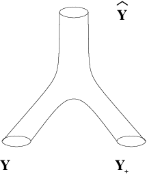
Proof of Lemma 4.9: Let $(z_{1},z_{2},z_{3},z_{4})$ be coordinates in $\mathbb{C}^{4}$ ; for every positive real number $r$ set:

M_{r}:=\left\{\mathbf{z}\in\mathbb{C}^{4}:\left|z_{1}\right|^{2}+\left|z_{2}\right|^{2}-\left|z_{3}\right|^{2}-\left|z_{4}\right|^{2}=r\right\}.

Then,

\begin{array}[]{cccc}\phi_{+}:&M_{r}&\longrightarrow&S^{3}\times\mathbb{C}^{2}\\ &\left(z_{1},z_{2},z_{3},z_{4}\right)&\longmapsto&(\frac{z_{1}}{\rho_{+}},\frac{z_{2}}{\rho_{+}},{z_{3}}\cdot{\rho_{+}},{z_{4}}\cdot{\rho_{+}})\end{array}

is an isomorphism, where $\rho_{+}:=\sqrt{\left|z_{1}\right|^{2}+\left|z_{2}\right|^{2}}=\sqrt{r+\left|z_{3}\right|^{2}+\left|z_{4}\right|^{2}}.$

Similarly for $M_{-r}$ . $\diamondsuit$

4.4. $\mathbf{M}$ –theory lifts and $\mathbf{M}$ –theory flops

Theorem 4.11.

[1, 2], [10], [11] There exists a commutative diagram

(100)

\begin{array}[]{ccc}M_{-r}&&M_{r}\\ {}_{\pi_{-}}\downarrow&&\downarrow_{\pi_{+}}\\ X_{-}&&X_{+}\\ {}_{h_{-}^{\left(N\right)}}\downarrow&&\downarrow_{h_{+}^{\left(N\right)}}\\ \mathbb{R}^{4}\times S^{2}&<-\mathit{conifold}->&S^{3}\times\mathbb{R}^{3}.\end{array}

where,

(1)

$M_{-r}$ and $M_{r}$ are as in Proposition 4.10.
(2)

$X_{-}$ and $X_{+}$ are $G_{2}$ holonomy spaces.
(3)

$(S^{3},0)\subset X_{+}$ is a locus of $A_{N-1}$ singularities.
(4)

The diagram is physically consistent, for large $N$ with the $\mathbf{M}$ –theory lift to $X_{-}$ (resp. $X_{+}$ ) of $N$ RR fluxes on $\mathcal{O}_{\mathbb{P}}^{1}(-1)\oplus\mathcal{O}_{\mathbb{P}}^{1}(-1)$ (resp. $\operatorname{SU}(N)$ branes on $T^{*}S^{3}$ ).
(5)

The surjections $h_{-}^{\left(N\right)},h_{+}^{\left(N\right)}$ give rise to the fluxes and branes, respectively, for the type II– $A$ string theories obtained by dimensional reduction on the two sides of the conifold transition.
(6)

$\mathbf{M}$ –theory compactified on $X_{-}$ is equivalent to $\mathbf{M}$ –theory on $X_{+}$ .

Thus, there is no “phase” transition between $X_{-}$ and $X_{+}$ , exactly as when II– $A$ is compactified on Calabi-Yau varieties related by a “flop” (see [112]).
Hence the term $\mathbf{M}$ –theory flop. This physics description is valid only for large $N$ .

The physics statement in [2], [10] and [11] is that the theory does not go through a singularity under the $\mathbf{M}$ –theory flop: this implies the Gopakumar-Vafa conjecture for the conifold transition.

Sketch of the proof: At the time of this lecture the works [1, 2], [10] were in print, while the main results of [11] had just been recently announced. The geometric lift $\left(\text{\ref{lift}}\right)$ gives an $\mathbf{M}$ –theory lift of II– $A$ string theories when $N=1$ . The singularity of the map $h_{+}$ denotes the presence of branes.

To get the $\mathbf{M}$ –theory lift with $N$ D–branes wrapped on $S^{3}\times\{0\}\subset S^{3}\times\mathbb{R}^{3}$ we need to introduce corresponding singularities on $M_{r}$ (see Section 4.2). We do so by defining a suitable action of the group of $N^{\text{th}}$ roots of unity on $\mathbb{C}^{4}$ : the induced action on $M_{-r}$ will give $N$ units of RR flux on $\mathbb{R}^{4}\times S^{2}$ .

Let $\Gamma_{N}:=\mathbb{Z}/N\mathbb{Z}$ act on $\mathbb{C}^{4}$ as

(101)

\begin{array}[]{lll}\Gamma\times\mathbb{C}^{4}&\longrightarrow&\mathbb{C}^{4}\\ \left(n,\mathbf{z}\right)&\longmapsto&\left(z_{1},z_{2},\xi_{n}z_{3},\xi_{n}z_{4}\right)\end{array}

where $\xi_{n}:=\exp\left(2\pi in/N\right).$ The complex plane $F=:\{z_{3}=z_{4}=0\}$ is the fixed locus of $\Gamma$ . Recall that $M_{-r}\cong{{\mathbb{C}^{2}}_{(z_{1},z_{2})}\times S^{3}}$ and $M_{r}\cong{S^{3}\times{\mathbb{C}^{2}}_{(z_{3},z_{4})}}$ . Then:

F\cap M_{-r}=\emptyset,\ \ F\cap M_{r}=S^{3}\times\left\{\mathbf{0}\right\}.

The quotient

M_{-r}\cong{\mathbb{C}^{2}}_{(z_{1},z_{2})}\times S^{3}\longrightarrow M_{-r}/\Gamma\cong{\mathbb{R}^{4}}\times(S^{3}/\Gamma):=X_{-}

is smooth; $(S^{3}/\Gamma)$ is called a lens space and is denoted by $L\left(N\right).$ Furthermore, since the $\Gamma$ –action restricts to the fiber of the Hopf fibration, the map $h_{-}$ in $\left(\text{\ref{lift}}\right)$ can be factorized through the canonical projection $\pi_{-}$ as follows

\begin{array}[]{lll}M_{-r}&\stackrel{{\scriptstyle h_{-}}}{{\longrightarrow}}&\mathbb{R}^{4}\times S^{2}\\ {}_{\pi_{-}}\searrow&&\nearrow_{h_{-}^{\left(N\right)}}\\ &X_{-}.&\end{array}

On the other hand the quotient

M_{r}\cong S^{3}\times{\mathbb{C}^{2}}_{(z_{3},z_{4})}\longrightarrow M_{r}/\Gamma\cong S^{3}\times\left({\mathbb{R}^{4}}/\Gamma\right):=X_{+}

contains an $S^{3}$ of singular points. Furthermore, since the $\Gamma$ –action restricts to the fiber of the Hopf fibration, the map $h_{+}$ in $\left(\text{\ref{lift}}\right)$ can topologically be factorized through the canonical projection as follows

\begin{array}[]{lll}M_{r}&\stackrel{{\scriptstyle h_{+}}}{{\longrightarrow}}&S^{3}\times\mathbb{R}^{3}\\ {}_{\pi_{+}}\searrow&&\nearrow_{h_{+}^{\left(N\right)}}\\ &X_{+}.&\end{array}

$\mathbb{R}^{4}/\Gamma$ is an $A_{N-1}$ singularity, with gauge group $SU(N)$ (see Appendix 5). In fact with the change of coordinates $w_{3}=z_{3},w_{4}=\sqrt{-1}\cdot\overline{z}_{4}$ , the action becomes: $(w_{3},w_{4})\to(\xi w_{3},\xi^{-1}w_{4})$ as described in Appendix 5. This is the geometric incarnation of the $\mathbf{M}$ –theory lift with $SU(N)$ –branes wrapped on $S^{3}$ (see Section 4.2).

Furthermore the non–singular $\mathbb{Z}_{N}$ –quotient (on the left of diagram $\left(\text{\ref{lift-N}}\right)$ ) gives rise to $N$ units of RR flux. In fact, if $V(-r)$ is the volume of $S^{3}\times\{\mathbf{0}\}$ , then $vol(S^{2})=vol(S^{3}/\Gamma)=V(-r)/N$ .

Recall that there exists a $G_{2}$ holonomy metric (see [24], [43]) on $M:=S^{3}\times\mathbb{R}^{4}$ . There is a precise description of the isometry group on $M$ and the action of $\Gamma$ is included in this subgroup. Hence the quotients $X_{-}$ and $X_{+}$ are also $G_{2}$ holonomy spaces.

It is worth pointing out that the equivalence of the theory and the relations between the physical parameters derived in [10] are only valid for large $N$ . The equivalence of the theories also implies the relations between Kähler modulus of $Y$ and the parameters of the Chern-Simons theory conjectured by Gopakumar and Vafa (see [10]).

On the other hand, the asympotics of the $G_{2}$ metric is not what would be expected from the II– $A$ situation; based on this observation Atiyah, Maldacena and Vafa conjectured the existence of a deformation of the $G_{2}$ metric with such properties (see [10]). This was later shown in [20]. $\diamondsuit$

5. Appendix: Some notation on singularities and their resolutions

Here we adopt the same notation and terminology introduced in [86], [87] and [88].

Definition 5.1.

A Weil divisor $D$ on a complex, normal and quasiprojective variety $\overline{Y}$ is $\mathbb{Q}$ -Cartier if, for some $r\in\mathbb{Z}$ , $rD$ is a Cartier divisor(i.e. $D\in Pic\left(\overline{Y}\right)\otimes\mathbb{Q}$ ).

If $\overline{Y}$ is smooth then any Weil divisor is Cartier.

Definition 5.2.

A $\overline{Y}$ be a complex, normal and quasiprojective variety is $\mathbb{Q}$ -factorial if any Weil divisor is $\mathbb{Q}$ -Cartier.

Definition 5.3.

Let $\overline{Y}$ be a complex, normal and quasiprojective variety and $K_{\overline{Y}}$ be its canonical divisor which is in general a Weil divisor. $\overline{Y}$ has canonical ( respectively terminal]) singularities if:

i)

$K_{\overline{Y}}$ is $\mathbb{Q}$ -Cartier.
ii)

given a smooth resolution $f:Y\longrightarrow\overline{Y}$ then

$rK_{Y}\equiv f^{*}K_{\overline{Y}}+\sum_{i}a_{i}E_{i}$

where $\equiv$ means “linearly equivalent”, $E_{i}$ are all the exceptional divisors of $f$ and $a_{i}\geq 0$ (respectively $a_{i}>0$ ).

The smallest integer $r$ for which such conditions hold is called the (global) index of $\overline{Y}$ and the smallest $r^{\prime}$ for which $r^{\prime}K_{\overline{Y}}$ is Cartier in a neighborhood of $P\in\overline{Y}$ is called the index of the singularity $P$ .

The divisor $\Delta:=\sum_{i}a_{i}E_{i}$ is called the discrepancy of the resolution $f$ .

If $\Delta\equiv 0$ then $f$ is called a crepant resolution of $\overline{Y}$ .

We are interested in transitions of Calabi-Yau manifolds: in particular, if at a point in the complex moduli space $\overline{Y}$ is singular and $K_{\overline{Y}}\equiv 0$ , its birational resolution should be crepant to preserve the Calabi-Yau condition on the canonical bundle.

Definition 5.4.

(see for example, [31])
By $NE(Y)\subset\mathbb{R^{\ell}}$ we denote the cone generated (over $\mathbb{R}_{\geq{0}}$ ) by the effective cycles of (complex) dimension 1, mod. numerical equivalence.
$\overline{NE(Y)}$ is the closure of $NE(Y)\subset\mathbb{R^{\ell}}$ in the finite dimensional real vector space $\mathbb{R^{\ell}}$ of all cycles of complex dimension 1, mod. numerical equivalence.

Note that $\ell=rk(Pic(Y))$ , and in the cases of Calabi-Yau manifolds, $\ell=b_{2}(Y)$ , the second Betti number of $Y$ .

Definition 5.5.

A birational contraction $f:Y\to\overline{Y}$ is called primitive extremal if the numerical class of a fiber of $f$ is on a ray of the Mori cone $NE(Y)$ .

Examples

The surface case. Let $X$ be a surface. It can be proved that a point $P\in X$ is a terminal singularity if and only if it is non-singular. Moreover the canonical (non--terminal) singular points are given by the Du Val singularities (DV points) which are classified as follows in terms of their local equations

$\displaystyle A_{n}$	$\displaystyle:$	$\displaystyle x^{2}+y^{2}+z^{n+1}=0\ ,\ n\geq 1$
$\displaystyle D_{n}$	$\displaystyle:$	$\displaystyle x^{2}+y^{2}z+z^{n-1}=0\ ,\ n\geq 4$
$\displaystyle E_{6}$	$\displaystyle:$	$\displaystyle x^{2}+y^{3}+z^{4}=0$
$\displaystyle E_{7}$	$\displaystyle:$	$\displaystyle x^{2}+y^{3}+yz^{3}=0$
$\displaystyle E_{8}$	$\displaystyle:$	$\displaystyle x^{2}+y^{3}+z^{5}=0$

In particular each of them admits a crepant resolution whose exceptional locus is composed of a set of $\left(-2\right)$ –curves (i.e. rational curves admitting self–intersection index $-2$ ) whose configurations are dually represented by the homonymous Dynkin diagrams: these are particular examples of Hirzebruch–Jung strings (see [14], chapters I and III).

Note that an ordinary double point is represented by $A_{1}$ and admits a crepant resolution whose exceptional locus is given by a unique $\left(-2\right)$ –curve. This equation is generalized to the threefold case in definition 1.4.

Each of the above singularities can be described as a quotient of $\mathbb{C}^{2}$ by a discrete subgroup $\Gamma\subset SL(2)$ . For $A_{n}$ , $\Gamma$ is the cyclic group of order $n+1$ generated by a primitive $n$ -th root of unity $\xi$ ; the action on $\mathbb{C}^{2}$ sends $(w_{1},w_{2})\to(\xi w_{1},\xi^{-1}w_{2})$ (see [96]).

The threefold case. Let $X$ be a threefold and $P\in X$ be a canonical singular point of index $r$ . A first important fact is that there exists a finite Galois covering $Y\longrightarrow X$ with group $\mathbb{Z}/r$ which is étale in codimension 1 and such that $Y$ is locally canonical of index 1 (see [86], corollary (1.9)).

Definition 5.6.

$P\in X$ is a compound Du Val singularity (cDV point) if the restriction to a surface section is a Du Val surface singularity.

The advantage of these kind of singularities is that they admit a simultaneous small resolution, as studied by several authors (see e.g. [87], [81], [74], [40]). The idea is that of thinking of an analytic neighborhood of an isolated cDV point as the total space of a 1–parameter family of deformations of the section over which we get a DV point. The total space of the induced 1–parameter family of deformations of a given resolution of such a DV point is then a small resolution of the starting cDV point. One can now apply the theory of simultaneous resolutions of DV points on surfaces [21], [22], [102].

The Main Theorem in [87] states that:

i)

$P\in X$ is a terminal singularity of index $r$ if and only if the local $r$ –fold cyclic covering $Y\longrightarrow X$ has only isolated compound Du Val singularities.
ii)

if $X$ admits at most canonical singularities then there exists a crepant partial resolution $S\longrightarrow X$ such that $S$ admits at most isolated terminal singularities.

These results allow one to reduce the problem of resolving canonical singularities to that of resolving cDV points, up to partial resolutions and finite coverings.

6. Appendix: More on the Greene-Plesser construction

Here we will quickly sketch an example supporting the Greene-Plesser construction explained in [27], [49] and [75].

Let $\overline{Y}_{1}$ be the degree 8 weighted hypersurface of ${\mathbb{P}}\left(1,1,2,2,2\right)$ and $Y_{1}$ be the desingularization induced by blowing up the singular locus of ${\mathbb{P}}\left(1,1,2,2,2\right)$ . Here $\phi$ is a primitive contraction of type $III$ and the transition can be completed by considering the embedding of ${\mathbb{P}}\left(1,1,2,2,2\right)$ in ${\mathbb{P}}^{5}$ by means of the linear system $\mathcal{O}\left(2\right)$ . The image of ${\mathbb{P}}\left(1,1,2,2,2\right)$ is a rank 3 hyperquadric of ${\mathbb{P}}^{5}$ . Hence the image of $\overline{Y}_{1}$ is the complete intersection of this hyperquadric with the generic quartic hypersurface of ${\mathbb{P}}^{5}$ . By smoothing the hyperquadric we get $\widehat{Y}_{1}$ . Following the idea of [49] the mirror partners may be found by taking the quotient with the subgroups of automorphisms preserving the holomorphic 3–form. Since the hypersurfaces’ cohomology can be completely described by means of Poincaré residues (see [50]) these subgroups are respectively given by

	$\displaystyle G$	$\displaystyle:$	$\displaystyle=\left\{\left(a_{0},\ldots,a_{4}\right)\in\left(\mathbb{Z}_{8}\right)^{2}\times\left(\mathbb{Z}_{4}\right)^{3}:\sum a_{i}\equiv 0\left(8\right)\right\}$
	$\displaystyle H$	$\displaystyle:$	$\displaystyle=\left\{\left(b_{0},\ldots,b_{5}\right)\in\left(\mathbb{Z}_{4}\right)^{2}\times\left(\mathbb{Z}_{2}\right)^{4}:b_{0}+b_{1}\equiv b_{2}+\cdots+b_{5}\equiv 0\left(4\right)\right\}.$

We denote by $a_{i},b_{j}$ the least non–negative integers representing the associated congruence class in $\mathbb{Z}_{n}$ . Hence the mirror partner $\widehat{Y}_{2}$ of $\widehat{Y}_{1}$ may be obtained by an $H$ –invariant complete intersection of bidegree $\left(2,4\right)$ in ${\mathbb{P}}^{5}$ via the desingularization of the quotient ${\mathbb{P}}^{5}/H$ where $H$ acts on ${\mathbb{P}}^{5}$ as follows

\begin{array}[]{lll}\left(H/\Delta_{H}\right)\times{\mathbb{P}}^{5}&\longrightarrow&{\mathbb{P}}^{5}\\ \left(\mathbf{b},\mathbf{x}\right)&\longmapsto&\left(\beta_{j}x_{j}\right)\end{array}

where

\beta_{j}:=\left\{\begin{array}[]{ll}\exp\left(\frac{b_{j}\pi i}{4}\right)&\text{ for }j=0,1\\ \pm 1&\text{ otherwise}\end{array}\right.

and $\Delta_{H}$ is the subgroup of $H$ giving a trivial action on ${\mathbb{P}}^{5}$ , i.e.

\Delta_{H}:=\left\{\left(0,\ldots,0\right),\left(2,2,1,\ldots,1\right)\right\}

On the other hand the mirror partner $Y_{2}$ of $Y_{1}$ may be obtained by a $G$ –invariant hypersurface of degree 8 in ${\mathbb{P}}\left(1,1,2,2,2\right)$ via the desingularization of the quotient ${\mathbb{P}}\left(1,1,2,2,2\right)/G$ where $G$ acts on ${\mathbb{P}}\left(1,1,2,2,2\right)$ as follows

\begin{array}[]{lll}G/\Delta_{G}\times{\mathbb{P}}\left(1,1,2,2,2\right)&\longrightarrow&{\mathbb{P}}\left(1,1,2,2,2\right)\\ \left(\mathbf{a},\mathbf{x}\right)&\longmapsto&\left(\alpha_{j}x_{j}\right)\end{array}

where

\alpha_{j}:=\left\{\begin{array}[]{ll}\exp\left(\frac{a_{j}\pi i}{8}\right)&\text{ for }j=0,1\\ \exp\left(\frac{a_{j}\pi i}{4}\right)&\text{ otherwise}\end{array}\right.

and $\Delta_{G}$ is the diagonal subgroup of $G$ , which is

\Delta_{G}:=\left\{\left(a,\ldots,a\right):0\leq a\leq 3\right\}

It can be checked that there is a birational equivalence between $\widehat{Y}_{2}$ and $Y_{2}$ representing a mirror partner of our transition.

7. Appendix: More on transitions in superstring theory

Strominger gave in [98] a physical explanation of how to resolve the conifold singularities of the moduli space of classical string vacua by means of massless Ramond--Ramond (RR) black holes. More precisely, the possible compactifications of a 10–dimensional II– $B$ string theory to 4 dimensions on a Calabi-Yau manifold $Y$ may be parametrized by the choice of the complex structure characterizing $Y$ . Such a choice may be described by the periods of a holomorphic 3–form $\Omega$ over a suitable symplectic basis of $H_{3}\left(Y,\mathbb{Q}\right)$ (see [34] and [97] for detailed notation in a $N=2$ , 4–dimensional supergravity theory and in special geometry) which can be considered as projective coordinates of the moduli space $\mathcal{M}\left(Y\right)$ of complex structures. The complex codimension 1 locus defined in $\mathcal{M}$ by the vanishing of one of those periods is composed of singular complex structures generically geometrically realized by a conifold. In fact the generic singularity is given by an ordinary double point. Note that the associated vanishing cycle is represented by the 3–cycle of the symplectic basis corresponding to the vanishing period.

Such singularities induce a polydromic behavior for the components of the self–dual 5–form giving the classical field. Following an analogous construction given in [93] and applied in the completely different context of $N=2$ supersymmetric Yang–Mills theory, Strominger resolved this problem by means of a low–energy effective Wilsonian field defined by including the light fields associated with extremal black 3–branes which can wrap around the vanishing 3–cycles and are always contained in a 10–dimensional compactified type II– $B$ theory (see [55]). These 3–branes represent black holes whose mass is proportional to the volume of the vanishing cycles they wrap around. Hence they are massless at the conifold and by integrating out the smooth so defined Wilsonian field we get exactly the polydromic behavior of the classical field. This is enough to ensure that the theory may be smoothly extended to the conifold.

On the other hand, in the case of a 10–dimensional compactified type II– $A$ theory we get a similar picture by taking the periods of a complexified Kähler form $\omega\in H^{2}\left(Y,\mathbb{C}\right)=H^{1,1}\left(Y\right)$ over a suitable basis of $H_{2}\left(Y,\mathbb{Q}\right)$ as projective coordinates of the moduli space $\mathcal{M}^{{}^{\prime}}\left(Y\right)$ of all possible Kähler structures on $Y$ (which parametrizes all the possible compactifications of a 10–dimensional II– $A$ string theory to 4 dimensions on the Calabi-Yau manifold $Y$ ). We now get black 2-branes (see [55]) which can wrap around vanishing 2–cycles and represent massless black holes at the conifold. Since in this case these massless states are a result of large instanton corrections the resolution of singularities can be obtained by passing to the dual II– $B$ compactification on a mirror model $Y^{\circ}$ of $Y$ and by proceeding as before.

8. Appendix: Principal bundles, connections etc

Here we review some terminology, concepts and properties from differential geometry: for more details see, for example, [53], [82] and [106].

Definition 8.1.

Let $G$ be a Lie group. A left ( resp. right) action of $G$ on a manifold $M$ is a homomorphism (resp. anti–homomorphism) to the group of diffeomorphisms of $M$

L\ \left(\text{resp. }R\right):G\longrightarrow Diff\left(M\right)

In particular for every $\sigma,\tau\in G$ we have $L\left(\sigma\right)$ $\circ L\left(\tau\right)=L\left(\sigma\tau\right)$ (resp. $R\left(\sigma\right)$ $\circ R\left(\tau\right)=R\left(\tau\sigma\right)$ ).

Definition 8.2.

An action is free if $id$ is the unique element of $G$ whose image in $Diff(M)$ admits a fiexd point. Note that if the $G$ –action is free then it is an injection of $G$ into $Diff\left(M\right)$ .

Definition 8.3.

A principal $G$ –bundle on a manifold $M$ is a manifold $P$ on which $G$ acts freely on the right together with a smooth, surjective map $\pi:P\rightarrow M$ such that

(1)

for every point $m\in M$ there is a local trivialization of $P$ i.e. an open neighborhood $\{U_{a}\}$ and a local diffeomorphism $\varphi_{U_{a}}:\pi^{-1}\left(U_{a}\right)\stackrel{{\scriptstyle\cong}}{{\rightarrow}}U_{a}\times G$ making the following diagram commutative

(102)

\begin{array}[]{ccc}\pi^{-1}\left(U\right)&\stackrel{{\scriptstyle\varphi_{U}}}{{\longrightarrow}}&U\times G\\ {}^{\pi}\downarrow&\stackrel{{\scriptstyle pr_{1}}}{{\swarrow}}&\\ U&&\end{array}

(2)

$\pi$ is $G$ –invariant i.e. for every $p\in P$ and every $\sigma\in G$

$\pi\left(p\sigma\right)=\pi\left(p\right)$

where $p\sigma:=R\left(\sigma\right)p$ .

Remark 8.4.

For a principal bundle $\left(P,\pi\right)$ the map $\pi$ is a submersion, implying that

\mathcal{V}_{p}P:=\ker\left(d_{p}\pi\right)=T_{p}\pi^{-1}\left(\pi\left(p\right)\right)

for every $p\in\pi^{-1}\left(\pi\left(p\right)\right)$ . Set $m:=\pi\left(p\right)\in M$ and let $\left(U,\varphi_{U}\right)$ be a local trivialization of $P$ near $m$ . The commutative diagram (102) allows us to define a diffeomorphism $\sigma_{m}^{U}$ such that

\left(\sigma_{m}^{U}\right)^{-1}:=\left(\varphi_{U}^{-1}\right)\mid_{\left\{m\right\}\times G}:G\stackrel{{\scriptstyle\cong}}{{\longrightarrow}}\pi^{-1}\left(m\right)

Its differential gives the isomorphism

d_{p}\sigma_{m}^{U}:T_{p}\pi^{-1}\left(m\right)\stackrel{{\scriptstyle\cong}}{{\longrightarrow}}T_{\sigma_{m}^{U}\left(p\right)}G

On the other hand by differentiating the automorphism $r_{\sigma}$ of $G$ , given by right multiplication by $\sigma\in G$ , we get the isomorphism

d_{id}r_{\sigma}:\mathfrak{g}\cong T_{id}G\stackrel{{\scriptstyle\cong}}{{\longrightarrow}}T_{\sigma}G

where $\mathfrak{g}$ is the Lie algebra associated with $G$ whose elements are all the left invariant vector fields on $G$ . Hence for every $p\in\pi^{-1}\left(m\right)$ we get the isomorphism

d_{p}\left(r_{\sigma_{m}^{U}\left(p\right)}^{-1}\circ\sigma_{m}^{U}\right):\ker\left(d_{p}\pi\right)\stackrel{{\scriptstyle\cong}}{{\longrightarrow}}\mathfrak{g}

This suffices to conclude that the vertical bundle $\mathcal{V}P$ associated with the principal $G$ –bundle $\left(P,\pi\right)$ is a vector bundle whose standard fibre is the Lie algebra $\mathfrak{g}$ associated with $G$ . In particular near a point $p\in P$ we have the local trivialization $\left(\pi^{-1}\left(U\right),\varphi_{\pi^{-1}\left(U\right)}\right)$ where

\varphi_{\pi^{-1}\left(U\right)}:\mathcal{V}P\mid_{\pi^{-1}\left(U\right)}\stackrel{{\scriptstyle\cong}}{{\longrightarrow}}\pi^{-1}\left(U\right)\times\mathfrak{g}

is the diffeomorphism defined by setting

\varphi_{\pi^{-1}\left(U\right)}\left(u\right):=\left(q,d_{q}\left(r_{\sigma_{\pi\left(q\right)}^{U}\left(q\right)}^{-1}\circ\sigma_{\pi\left(q\right)}^{U}\right)\left(u\right)\right)

for every $q\in\pi^{-1}\left(U\right)$ and $u\in\mathcal{V}_{q}P$ .

Recall the definition 2.2 of a connection on a principal $G$ –bundle $\left(P,\pi\right)$ . It is not difficult to show that every principal bundle on a paracompact manifold $M$ admits a connection (see e.g. [82], theorems 2.35 and 9.3). Given a connection $\mathcal{H}P\subset TP$ we can uniquely split a vector field $X:P\longrightarrow TP$ into a horizontal part $\mathcal{H}X:P\longrightarrow\mathcal{H}P$ and a vertical part $\mathcal{V}X:P\longrightarrow$ $\mathcal{V}P$ such that for every $p\in P$

(103)

X_{p}=\mathcal{H}_{p}X+\mathcal{V}_{p}X

Recalling definition 2.3 let $A\in\Omega^{1}\left(P,\mathfrak{g}\right)$ be the $\mathfrak{g}$ –valued 1–form associated with the connection $\mathcal{H}P$ and $\ \Omega\in\Omega^{2}\left(P,\mathfrak{g}\right)$ be its curvature $\mathfrak{g}$ –valued 2–form. These forms are related to each other by the structure equation

\Omega\left(X,Y\right)=dA\left(X,Y\right)+\left[AX,AY\right]

for any vector fields $X,Y$ on $P$ . We can rewrite it in the following shorter form

(104)

\Omega=dA+\frac{1}{2}\left[A,A\right]

by setting $\left[A,A\right]\left(X,Y\right):=\left[AX,AY\right]-\left[AY,AX\right]$ .

Let $l_{\sigma}$ be the automorphism of $G$ given by left multiplication by $\sigma\in G$ . The dual vector space $\mathfrak{g}^{*}$ of the Lie algebra $\mathfrak{g}$ can be canonically identified with the vector space of all left invariant $1$ –forms on $G$ since all such forms assume constant values on left invariant vector fields. The composition

a_{\sigma}:=l_{\sigma}\circ r_{\sigma^{-1}}:G\longrightarrow G

is an automorphism of $G$ fixing $id\in G$ . Therefore its differential

(105)

Ad_{\sigma}:=d_{id}a_{\sigma}

may be thought as an automorphism of $\mathfrak{g}\cong T_{id}G$ and its codifferential $\delta_{id}a_{\sigma}$ as an automorphism of $\mathfrak{g}^{*}$ .

Proposition 8.5.

Let us consider $\theta\in\mathfrak{g}^{*}$ and $X,Y\in\mathfrak{g}$ . Then for every $\sigma\in G$

(106)

\left(\delta r_{\sigma}\right)\theta X=\left(\theta\circ Ad_{\sigma}\right)X

and they satisfy the Maurer--Cartan equation¹¹ 1 For this reason left invariant 1–forms are also called Maurer–Cartan forms.

(107)

d\theta\left(X,Y\right)=-\theta\left[X,Y\right]

Proof. To prove $\left(\text{\ref{adj-transf}}\right)$ note that for every $\tau\in G$ left invariance of $\theta$ gives

\theta_{\tau\sigma}=\left(\delta_{\tau\sigma}l_{\sigma^{-1}}\right)\theta_{\sigma^{-1}\tau\sigma}

which implies

\left(\delta_{\tau}r_{\sigma}\right)\theta_{\tau\sigma}=\left(\delta_{\tau}r_{\sigma}\circ\delta_{\tau\sigma}l_{\sigma^{-1}}\right)\theta_{\sigma^{-1}\tau\sigma}=\left(\delta_{\tau}a_{\sigma^{-1}}\right)\theta_{\sigma^{-1}\tau\sigma}=\theta_{\sigma^{-1}\tau\sigma}\circ d_{\tau}a_{\sigma}

To restrict this relation to a left invariant vector field $X\in\mathfrak{g}$ means to choose $\tau=id$ and so to obtain just $\left(\text{\ref{adj-transf}}\right)$ . For $\left(\text{\ref{MCeqn}}\right)$ let us observe that almost by definition

d\theta\left(X,Y\right)=X\theta Y-Y\theta X-\theta\left[X,Y\right]

Since $X,Y\in\mathfrak{g}$ left invariance of $\theta$ implies that both $\theta Y$ and $\theta X$ are constant functions. This suffices to finish the proof. $\diamondsuit$

Given a point $p\in P$ let us now consider the codifferential

\delta\lambda_{p}:T^{*}P\longrightarrow T^{*}G

and let $A$ be the connection form of $\mathcal{H}P$ . We can then define the $\mathfrak{g}$ –valued 1–form $\left(\delta\lambda\right)A\in\Omega^{1}\left(G,\mathfrak{g}\right)$ by setting

(108)

\left(\left(\delta\lambda\right)A\right)_{\sigma}:=\left(\delta_{\sigma}\lambda_{p}\right)A_{p\sigma}

for every $\sigma\in G$ . This definition is not dependent on the choice of $p\in P$ since by $\left(\text{\ref{g-connection}}\right)$ we have for every $v\in T_{\sigma}G$

\left(\delta_{\sigma}\lambda_{p}\right)A_{p\sigma}\left(v\right)=A_{p\sigma}\left(\left(d_{\sigma}\lambda_{p}\right)v\right)=\left(d_{id}\lambda_{p\sigma}\right)^{-1}\left(\mathcal{V}_{p\sigma}\left(d_{\sigma}\lambda_{p}\right)v\right)

Since $\lambda_{p}$ is a diffeomorphism of $G$ onto the fiber $\pi^{-1}\left(\pi\left(p\right)\right)$ it follows that $\left(d_{\sigma}\lambda_{p}\right)v\in\mathcal{V}_{p\sigma}P$ and

(109)

\left(\delta_{\sigma}\lambda_{p}\right)A_{p\sigma}\left(v\right)=\left(d_{id}\lambda_{p\sigma}\right)^{-1}\left(\left(d_{\sigma}\lambda_{p}\right)v\right)=d_{\sigma}\left(\lambda_{p\sigma}^{-1}\circ\lambda_{p}\right)v=\left(d_{id}l_{\sigma}\right)^{-1}v

where the last equality follows by differentiating the commutative diagram

\begin{array}[]{lll}G&\stackrel{{\scriptstyle\lambda_{p}}}{{\longrightarrow}}&P\\ {}_{l_{\sigma^{-1}}}\searrow&&\swarrow_{\lambda_{p\sigma}^{-1}}\\ &G&\end{array}

The $\mathfrak{g}$ –valued 1–form $\left(\delta\lambda\right)A$ is actually left invariant since

\delta_{\sigma}l_{\tau}\left(\left(\delta\lambda\right)A\right)_{\tau\sigma}=\left(\delta_{\sigma}l_{\tau}\circ\delta_{\tau\sigma}\lambda_{p}\right)A_{p\tau\sigma}=A_{p\tau\sigma}\circ d_{\sigma}\left(\lambda_{p}\circ l_{\tau}\right)

and given $v\in T_{\sigma}G$ we get

	$\displaystyle\delta_{\sigma}l_{\tau}\left(\left(\delta\lambda\right)A\right)_{\tau\sigma}v$	$\displaystyle=$	$\displaystyle\left(d_{id}\lambda_{p\tau\sigma}\right)^{-1}\left(\mathcal{V}_{p\tau\sigma}d_{\sigma}\left(\lambda_{p}\circ l_{\tau}\right)v\right)=$
			$\displaystyle d_{\sigma}\left(\lambda_{p\tau\sigma}^{-1}\circ\lambda_{p}\circ l_{\tau}\right)v=\left(d_{id}l_{\sigma}\right)^{-1}v=\left(\left(\delta\lambda\right)A\right)_{\sigma}v$

Therefore $\left(\delta\lambda\right)A\in\mathfrak{g}^{*}\otimes\mathfrak{g}\cong Hom\left(\mathfrak{g},\mathfrak{g}\right)$ : call it the Maurer–Cartan form associated with the connection $\mathcal{H}P$ . By $\left(\text{\ref{l.i.ext}}\right)$ it is the $\mathfrak{g}$ –valued 1–form which assigns to each tangent vector to $G$ its left invariant extension: hence its representative in $Hom\left(\mathfrak{g},\mathfrak{g}\right)$ is the identity $id_{\mathfrak{g}}$ and the Maurer–Cartan equation $\left(\text{\ref{MCeqn}}\right)$ gives

d\left(\delta\lambda\right)A\left(X,Y\right)=-\left(\delta\lambda\right)A\left[X,Y\right]=-\left[X,Y\right]=-\left[\left(\delta\lambda\right)AX,\left(\delta\lambda\right)AY\right]

Then we get

d\left(\delta\lambda\right)A+\frac{1}{2}\left[\left(\delta\lambda\right)A,\left(\delta\lambda\right)A\right]=0

By defining $\left(\delta\lambda\right)\Omega$ just like we did for $\left(\delta\lambda\right)A$ in $\left(\text{\ref{MCconnection}}\right)$ the structure equation $\left(\text{\ref{struct.eqn}}\right)$ and the last one allows us to conclude that

(110)

\left(\delta\lambda\right)\Omega=0

Since $\delta_{id}\lambda_{p}$ realizes the isomorphism $\mathcal{V}_{p}^{*}P\cong\mathfrak{g}^{*}$ this actually means that the curvature 2–form $\Omega$ vanishes on the tangent space to the fiber of $P$ . Hence the structure equation $\left(\text{\ref{struct.eqn}}\right)$ can be rewritten as follows:

dA=\Omega-\frac{1}{2}\left[A,A\right]

to give a decomposition of $dA$ into horizontal and vertical parts.

Let us now come back to consider the connection form $A$ of $\mathcal{H}P$ . It can be defined as in $\left(\text{\ref{g-connection}}\right)$ since the connection $\mathcal{H}P$ determines a splitting in the tangent bundle $TP$ . But also the converse is true and the connection $\mathcal{H}P$ may be obtained by the $\mathfrak{g}$ –valued 1–form $A$ just like the vector sub–bundle $\ker A$ .

Proposition 8.6.

If $A$ is the connection form of a connection $\mathcal{H}P$ then

(111)		$\displaystyle\forall p\in P,\forall u\in\mathcal{V}_{p}P\qquad\left(d_{id}\lambda_{p}\right)A_{p}u=u$
	$\displaystyle\forall\sigma\in G\qquad\delta R\left(\sigma\right)A=Ad_{\sigma^{-1}}\circ A$

Conversely, given a $\mathfrak{g}$ –valued $1$ –form $A$ on $P$ satisfying these conditions the vector sub–bundle $\ker A\subset TP$ gives a connection on $P$ whose connection form is $A$ . Hence the set $\mathcal{A}$ _P of all connections on $P$ can be identified with the affine subspace of $\Omega^{1}\left(P,\mathfrak{g}\right)$ defined by conditions $\left(\text{\ref{conditions}}\right)$ .

Furthermore the curvature form $\Omega\in\Omega^{2}\left(P,\mathfrak{g}\right)$ of $\mathcal{H}$ $P$ is a $\mathfrak{g}$ –valued $2$ –form such that

(112)		$\displaystyle\forall p\in P,\forall u,v\in\mathcal{V}_{p}P\qquad\Omega_{p}(u,v)=0$
	$\displaystyle\forall\sigma\in G\qquad\delta R\left(\sigma\right)\Omega=Ad_{\sigma^{-1}}\circ\Omega$

Proof. The first equality in $\left(\text{\ref{conditions}}\right)$ follows immediately by the definition of the connection form $A$ . For the second one note that

\delta_{p}R\left(\sigma\right)A_{p\sigma}\left(u\right)=A_{p\sigma}\left(d_{p}R\left(\sigma\right)u\right)=\left(d_{id}\lambda_{p\sigma}\right)^{-1}\mathcal{V}_{p\sigma}\left(d_{p}R\left(\sigma\right)u\right)

The condition $\left(\text{\ref{G-invariance}}\right)$ for the connection $\mathcal{H}P$ implies that $\mathcal{V}_{p\sigma}\left(d_{p}R\left(\sigma\right)u\right)=d_{p}R\left(\sigma\right)\left(\mathcal{V}_{p}u\right)$ . On the other hand $\mathcal{V}_{p}u=d_{id}\lambda_{p}\left(A_{p}u\right)$ and we can write

\delta_{p}R\left(\sigma\right)A_{p\sigma}\left(u\right)=\left(d_{id}\lambda_{p\sigma}\right)^{-1}\circ d_{p}R\left(\sigma\right)\circ d_{id}\lambda_{p}\left(A_{p}u\right)=Ad_{\sigma^{-1}}\circ A\left(u\right)

where the last equality follows by the commutative diagram

\begin{array}[]{ccc}\pi^{-1}\left(\pi\left(p\right)\right)&\stackrel{{\scriptstyle R\left(\sigma\right)}}{{\longrightarrow}}&\pi^{-1}\left(\pi\left(p\sigma\right)\right)\\ {}_{\lambda_{p}}\uparrow&&\downarrow_{\lambda_{p\sigma}^{-1}}\\ G&\stackrel{{\scriptstyle a_{\sigma^{-1}}}}{{\longrightarrow}}&G\end{array}

For the converse it suffices to observe that the first equality in $\left(\text{\ref{conditions}}\right)$ gives the splitting condition $\left(\text{\ref{splitting}}\right)$ and the second one ensures the $G$ –invariance $\left(\text{\ref{G-invariance}}\right)$ for $\ker A$ . Hence it is a connection on $P$ whose connection form is clearly $A$ .

Finally the first equality in $\left(\text{\ref{curv-conditions}}\right)$ follows by $\left(\text{\ref{MCcurvature}}\right)$ and the second one by applying the second equality in $\left(\text{\ref{conditions}}\right)$ to the definition $\left(\text{\ref{g-curvature}}\right)$ of $\Omega$ .

Let us recall that a gauge transformation of $P$ is an automorphism $\varphi$ of $P$ which induces the identity map on the base manifold $M$ . Then it leaves every fibre fixed and it makes sense to define the associated map

(113)

\sigma_{\varphi}:P\longrightarrow G

such that $\varphi\left(p\right)=p\sigma_{\varphi}\left(p\right)$ . By applying the Leibniz rule to the connection form $A$ we get that

\left(\delta_{p}\varphi\right)A_{\varphi\left(p\right)}=\delta_{p}R\left(\sigma_{\varphi}\left(p\right)\right)A_{p\sigma_{\varphi}\left(p\right)}+\left(\delta_{p}\sigma_{\varphi}\right)\left(\delta\lambda\right)A_{\sigma_{\varphi}\left(p\right)}

where $\left(\delta\lambda\right)A$ is the Maurer-Cartan form of the given connection. The second equation in $\left(\text{\ref{conditions}}\right)$ allows us to conclude that under a gauge transformation $\varphi$ the connection form $A$ behaves as follows:

(114)

\left(\delta\varphi\right)A=Ad_{\sigma_{\varphi}^{-1}}\circ A+\left(\delta\sigma_{\varphi}\right)\left(\delta\lambda\right)A

If $\Omega$ is the associated curvature then by $\left(\text{\ref{MCcurvature}}\right)$ and $\left(\text{\ref{curv-conditions}}\right)$ it transforms under $\varphi$ as follows:

(115)

\left(\delta\varphi\right)\Omega=Ad_{\sigma_{\varphi}^{-1}}\circ\Omega

Since gauge transformations on $P$ form a group $\mathcal{G}_{P}$ with respect to the composition, $\left(\text{\ref{gauge on connection}}\right)$ defines an action of $\mathcal{G}_{P}$ on the affine space of connections $\mathcal{A}_{P}$ .

Let us now consider the exponential map $\exp:\mathfrak{g}\longrightarrow G$ which assigns to a left invariant vector field $X\in\mathfrak{g}$ the point $\exp_{X}\left(1\right)\in G$ where $\exp_{X}\left(t\right)$ is the unique 1–parameter group whose tangent vector at $0\in\mathbb{R}$ is $X_{id}\in T_{id}G$ . Since $Ad_{\sigma}\in$ Aut $\left(\mathfrak{g}\right)$ , for every $\sigma\in G$ , and the Lie algebra of Aut $\left(\mathfrak{g}\right)$ is End $\left(\mathfrak{g}\right)$ we get the following commutative diagram:

\begin{array}[]{ccc}G&\stackrel{{\scriptstyle Ad}}{{\longrightarrow}}&\text{Aut}\left(\mathfrak{g}\right)\\ {}_{\exp}\uparrow&&\uparrow_{\exp}\\ \mathfrak{g}&\stackrel{{\scriptstyle ad}}{{\longrightarrow}}&\text{End}\left(\mathfrak{g}\right)\end{array}

where $ad:=d\left(Ad\right)$ .

Definition 8.7.

For every $X,Y\in\mathfrak{g}$ the symmetric bilinear form

\left\langle X,Y\right\rangle:=\text{tr}\left(ad_{X}\circ ad_{Y}\right)

is called the Killing form of the lie algebra $\mathfrak{g}$ .

Given a point $m\in M$ recall the definition $\left(\text{\ref{Hol(m)}}\right)$ of the holonomy group Hol ${}_{\mathcal{H}P}\left(m\right)$ of a connection $\mathcal{H}$ $P$ at $m\in M$ . If the base manifold $M$ is connected all these groups are isomorphic when $m$ varies in $M$ since we can send

(116)

h_{\gamma}\in\text{Hol}_{\mathcal{H}P}\left(m_{1}\right)\longmapsto h_{\alpha*\gamma*\overline{\alpha}}\in\text{Hol}_{\mathcal{H}P}\left(m_{2}\right)

where $\alpha$ is a path from $m_{1}$ to $m_{2}$ and $\overline{\alpha}$ its reversed path. Then it make sense to define the holonomy group Hol_HP of the connection $\mathcal{H}$ $P$ .

9. Appendix: More on Witten’s open string theory interpretation of QFT

Sketch of proof of Theorem 3.2: We have to show that under the assumptions $\left(\text{\ref{ctg.hyp.}}\right)$ and $\left(\text{\ref{bdr.cond.}}\right)$ the weak coupling limit of the abstract string Lagrangian reduces exactly to the Lagrangian of a QFT on $L$ .

The low energy (or weak coupling) limit of a string theory is only approximated by a QFT since the limit Lagrangian admits perturbative corrections depending on the coupling constant and non–constant instanton corrections (see definition 3.8). The string theory analyzed in [111] is a topological theory given by an $A$ –twisted sigma model. At first Witten observes that this model does not depend on the coupling constant of the theory, implying that there cannot be any perturbative correction in the limit Lagrangian.

It remains then to show that all the non–constant instanton contributions vanish. Let $\sigma$ be the canonical symplectic form on $\widehat{Y}=T^{*}L$ . It is the differential of the Liouville form, i.e. in local canonical coordinates $\sigma=d\vartheta$ where $\vartheta:=\sum_{j=1}^{3}p_{j}dq_{j}$ . The Liouville form vanishes on $L$ given by $p_{1}=p_{2}=p_{3}=0$ . Note that the bosonic sigma model action reduces for instantons to be

I=\int_{\Sigma}\phi^{*}\left(\sigma\right)

Stokes’ theorem and condition $\left(\text{\ref{bdr.cond.}}\right)$ suffice to conclude that

(117)

I\left(\phi\right)=0

for all instantons $\phi$ . On the other hand by its definition the bosonic sigma model action $I$ vanishes only for constant instantons. Hence we can admit only constant instanton corrections and the abstract string Lagrangian reduces exactly to the Lagrangian of the QFT on $L$ realizing the low energy limit. In the $A$ –twisted case such a limit turns out to be exactly a Chern–Simons $U\left(N\right)$ –gauge theory.

Dropping assumption $\left(\text{\ref{ctg.hyp.}}\right)$ . The main result of [111] is more general than Theorem 3.2. In fact he analyzes (section 4.4) the low energy limit of an $A$ –twisted topological open string theory whose target space is given by a Calabi–Yau threefold $\widehat{Y}$ admitting $L$ as a Lagrangian submanifold.

Theorem 9.1.

Let $\widehat{Y}$ be a local Calabi–Yau threefold and $L\subset\widehat{Y}$ a Lagrangian submanifold. Then there exist topological string theories with $\widehat{Y}$ as target space, such that their open sectors are equivalent to a QFT on $L$ up to the convergence of non–constant instanton contributions. In the $A$ –twisted case the Lagrangian action of the limit QFT is (if convergent) a deformation of a Chern–Simons action.

This result follows by assuming the same boundary conditions as above. But now $\left(\text{\ref{bdr.cond.}}\right)$ is no longer sufficient to conclude the vanishing $\left(\text{\ref{vanishing}}\right)$ for non–constant instantons: given $\phi$ , its instanton number is

q\left(\phi\right):=\int_{\Sigma}\phi^{*}\left(\omega\right)

where $\omega$ is the symplectic form of $\widehat{Y}$ . Instanton numbers turn out to be non–negative. For any knot $\mathcal{K}\subset\phi\left(\partial\Sigma\right)\subset L$ consider the Wilson line $W_{\mathcal{K}}^{R}$ constructed by holonomy on $L$ . For a given connection $A$ on a $U\left(N\right)$ –principal bundle Witten shows that the instanton contribution of $\phi$ is given by

-\frac{i\eta\left(\phi\right)e^{-\theta q\left(\phi\right)}}{2\pi k}\sum_{\mathcal{K}\subset\phi\left(\partial\Sigma\right)}\log\left(\text{ tr}_{R}\left(h_{\mathcal{K}}\right)\right)

where $\theta$ is a positive real parameter, $e^{-\theta q\left(\phi\right)}$ a suitable weighting factor and $\eta\left(\phi\right)=\pm 1$ . If $S\left(\mathcal{L}\left(A\right)\right)$ is the Chern–Simons action on $L$ the limit action turns out to be

(118)

S^{\prime}=S\left(\mathcal{L}\left(A\right)\right)-\frac{i}{2\pi k}\sum_{\phi}\left[\eta\left(\phi\right)e^{-\theta q\left(\phi\right)}\sum_{\mathcal{K}\subset\phi\left(\partial\Sigma\right)}\log\left(\text{ tr}_{R}\left(h_{\mathcal{K}}\right)\right)\right]

Under suitable assumptions on the “moduli space” of instantons $\phi$ the sum can be perturbatively evaluated for $\theta\gg 0$ .

Corollary 9.2.

Assume that $\widehat{Y}=T^{*}S^{3}$ and $L=\mathcal{C}$ is the Lagrangian submanifold given by the conormal bundle of the unknot knot in $S^{3}$ like in Proposition 3.13. Then the low energy limit QFT on $\mathcal{C}$ of the open sector of a type II– $A$ string theory with $M$ D–branes wrapped around $\mathcal{C}$ is a $SU\left(M\right)$ –Chern–Simons gauge theory on $\mathcal{C}$ . Moreover the global open string theory with $N$ D–branes wrapped around $S^{3}$ and $M$ D–branes wrapped around $\mathcal{C}$ admits a low energy limit QFT whose action is the following deformation of the $SU\left(M\right)$ Chern–Simons action on $\mathcal{C}$ :

S^{\prime}=S\left(\mathcal{L}\right)-\frac{i}{2\pi k}\sum_{d}\eta_{d}\log\left(\text{ tr}_{R}\left(h_{\mathcal{K}}^{d}\right)\right)

The first part of the statement can be proved like Theorem 3.2 since the Liouville form of $\mathbb{R}^{8}\supset T^{*}S^{3}$ vanishes when restricted to $\mathcal{C}$ , as in $\left(\text{\ref{lagrangian}}\right)$ . That is enough to guarantee the vanishing $\left(\text{\ref{vanishing}}\right)$ .

To prove the second part, note that the only non–trivial non–constant contributions come from instantons $\phi$ such that $\phi\left(\partial\Sigma\right)$ is a $d$ –covering of the unknot in $S^{3}$ . For these instantons $q\left(\phi\right)=0$ by Stokes’ theorem and the statement follows by $\left(\text{\ref{deformedCS}}\right)$ .

References

[1] Acharya BS 1999 M theory, Joyce orbifolds and super Yang-Mills Adv.Theor.Math.Phys. 3 227–248; hep--th/9812205.
[2] Acharya BS 2000 On realizing N=1 super Yang-Mills in M theory 1–16 hep--th/0011089
[3] Aganagic M, Klemm A, Vafa C 2001 “Disc instantons, mirror symmetry and the duality web” Z. Naturforsch. A57 1-28 (2002) ; hep–th/0105045.
[4] Altmann, K. 1997, The versal deformation of an isolated toric singularity Invent. Math.128, no. 3, 443–479.
[5] Aspinwall PS and Morrison DR 1993 Topological field theory and rational curves Commun. Math. Phys. 151 245–262.
[6] Atiyah MF 1989 “Topological quantum field theories” Publ. Math. I.H.E.S. 68 175–186.
[7] Atiyah MF 1990 The geometry and physics of knots Cambridge University Press.
[8] Atiyah MF 1990 “On framing of 3–manifolds” Topology 29 1–8.
[9] Atiyah MF and Bott R 1982 “The Yang–Mills equations over Riemann surfaces” Phil. Trans. R. Soc. Lond. A 308 523–615.
[10] Atiyah MF, Maldacena J and Vafa C 2001 An M–theory flop as a large $N$ duality J.Math.Phys. 42 3209-3220.
[11] Atiyah MF and Witten E 2001 “ $M$ –theory dynamics on a manifold of $G_{2}$ holonomy” hep–th/0107177.
[12] Avram A, Candelas P, Jančić D and Mandelberg 1996 “On the connectedness of the moduli space of Calabi–Yau manifolds” Nucl. Phys. B 465 458–472; hep–th/9511230.
[13] Axelrod S, Della Pietra S and Witten E 1991 “Geometric quantization of Chern–Simons gauge theory” J. Diff. Geom. 33 787–902.
[14] Barth W, Peters C and Van de Ven A 1984 Compact complex surfaces Springer–Verlag.
[15] Batyrev V, Ciocan-Fontanine I, Kim B and van Straten D 1998 “Conifold transitions and mirror symmetry for Calabi-Yau complete intersections in Grassmannians” Nucl. Phys. B 514 640–666; alg–geom/9710022.
[16] Berglund P, Katz S and Klemm A 1995 “Mirror symmetry and the moduli space for generic hypersurfaces in toric varieties” Nucl. Phys. B456 153–204.
[17] Berglund P, Katz S, Klemm A and Mayr P 1997 “New Higgs transition between dual $N=2$ string models” Nucl. Phys. B483 209–228.
[18] Bershadsky M, Cecotti S, Ooguri H and Vafa C 1993 “Holomorphic anomalies in topological field theories” (appendix by Katz S) Nucl. Phys. B 405 279–304 and in Mirror symmetry II AMS/IP Stud. Adv. Math. 1 655–682; hep–th/9302103.
[19] Bershadsky M, Cecotti S, Ooguri H and Vafa C 1994 “Kodaira–Spencer theory of gravity and exact results for quantum string amplitudes” Commun. Math. Phys. 165 311–428; hep–th/9309140.
[20] Brandhuber A, Gomis J, Gubser SS and Gukov S 2001 “Gauge theory at large $N$ and new $G_{2}$ holonomy metrics” Nucl. Phys. B 611 179–204; hep–th/0106034.
[21] Brieskorn E 1966 “Über die Auflösung gewisser Singularitäten von holomorphen Abbildungen” Math. Ann. 166 76–102.
[22] Brieskorn E 1968 “Die Auflösung der rationalitaten Singularitäten holomorpher Abbildungen” Math. Ann. 178 255–270.
[23] Bryant RL 1987 “Metrics with exceptional holonomy” Ann. of Math. 126 525–576.
[24] Bryant RL and Salamon SM 1989 “On the construction of some complete metrics with exceptional holonomy” Duke Math. J. 58 829–850.
[25] Candelas P, de la Ossa XC, 1990 “Comments on conifolds”Nucl. Phys. B 342, n.1, 246–268.
[26] Candelas P, de la Ossa XC, Green PS and Parkes L 1991 “A pair of Calabi–Yau manifolds as an exactly soluble superconformal theory” Nucl. Phys. B 359 21–74 and in Essays on mirror manifolds International Press 31–95.
[27] Candelas P, de la Ossa XC, Font A, Katz S and Morrison DR 1994 “Mirror symmetry for two parameter models, I” Nucl. Phys. B416 481–538.
[28] Chern S, Simons J 1974 “Characteristic forms and geometric invariants” Ann. Math. 99, 48–69.
[29] Chiang T–M, Greene B, Gross M and Kanter Y 1996 “Black hole condensation and the web of Calabi–Yau manifolds” Nucl. Phys. Proc. Supp. 46 82–95; hep–th/9511204.
[30] Clemens C. H. 1983 “Double Solids” Adv. in Math. 47 107–230.
[31] H. Clemens, J. Kollár, S. Mori 1988 “Higher Dimensional Geometry” “Asterisque” 166
[32] Cox AD and Katz S 1999 Mirror Symmetry and Algebraic Geometry vol. 68 Math. Surveys and Monographs (American Mathematical Society).
[33] Deligne P, Etingof P, Freed DS, Jeffrey LC, Kazhdan D, Morgan JW, Morrison D and Witten E eds. 1999 Quantum fields and strings: a course for mathematicians I, II Americam Mathematical Society, IAS.
[34] de Wit B, Lauwers P and van Proeyen A 1985 “Lagrangians of $N=2$ supergravity–matter systems” Nucl. Phys. B255 569–608.
[35] Donaldson SK 1983 “A new proof of a theorem of Narasimhan and Seshadri” J. Diff. Geom. 18 269–277.
[36] Douglas M, Katz S and Vafa C 1997 “Small instantons, del Pezzo surfaces and type $I^{\prime}$ theory” Nucl. Phys. B 497 155–172.
[37] Faber C and Pandharipande R 2000 “Hodge integrals and Gromov–Witten theory” Invent. Math. 139 173–199; math.AG/9810173.
[38] Freed DS 1995 “Classical Chern–Simons theory, Part 1” Adv. Math. 113 237–303.
[39] Freyd P, Yetter D, Hoste J, Lickorish WBR, Millett K and Ocneanu A 1985 “A new polynomial invariant of knots and links” Bull. AMS 12 183–312.
[40] Friedman R 1986 “Simultaneous resolution of threefold double points” Math. Ann. 274 671–689.
[41] Fulton W and Pandharipande R 1995 “Notes on stable maps and quantum cohomology” in Algebraic Geometry–Santa Cruz 1995 Proc. Sym. Pure Math. 62 Part 2, AMS, 45–96.
[42] Getzler E and Pandharipande R 1998 “Virasoro constraints and the Chern classes of the Hodge bundle” math.AG/9805114.
[43] Gibbons GW, Page DN and Pope CN 1990 “Einstein metrics on $S^{3},\mathbb{R}^{3}$ and $\mathbb{R}^{4}$ bundles” Commun. Math. Phys. 127 529–553.
[44] Gopakumar R and Vafa C 1998 “ $M$ –theory and topological strings–I” hep–th/9809187
[45] Gopakumar R and Vafa C 1998 “ $M$ –theory and topological strings–II” hep–th/9812127
[46] Gopakumar R and Vafa C 1999 “On the gauge theory/geometry correspondence” Adv.Theor.Math.Phys. 3 1415–1443.
[47] Graber T and Pandharipande R 1999 “Localization of virtual classes” Invent. Math. 135 487-518.
[48] Greene B, Morrison DR and Strominger A 1995 “Black hole condensation and the unification of string vacua” Nucl. Phys. B451 109–120.
[49] Greene B and Plesser MR 1990 “Duality in Calabi–Yau moduli space” Nucl. Phys. B338 15–37.
[50] Griffiths P 1969 “On the periods of certain rational integrals I, II” Ann. of Math. 90 460–495, 498–541.
[51] Gross M 1997 “Deforming Calabi–Yau threefolds” Math. Ann. 308 2, 187–220.
[52] Gross M 1997 “Primitive Calabi-Yau threefolds” J. Diff. Geom. 45 288–318.
[53] Helgason S 1978 Differential geometry, Lie groups and symmetric spaces Academic Press, New York.
[54] Hitchin NJ 1990 “Flat connections and geometric quantization” Commun. Math. Phys. 131 347–380.
[55] Horowitz G, Strominger A 1991 “Black Strings and $p$ –branes” Nucl. Phys. B360 197–209.
[56] Hosono S, Klemm A, Theisen S and Yau ST 1995 “Mirror symmetry, mirror map and applications to complete intersection Calabi–Yau spaces” Nucl. Phys. B433 501–554 and in Mirror symmetry II AMS/IP Stud. Adv. Math. 1 545–606; hep–th/9406055.
[57] Jones V 1985 “A polynomial invariant for knots via von Neumann algebras” Bull. AMS 12 103–111.
[58] Jones V 1987 “Hecke algebras representations of braid groups and link plynomials” Ann. Math 126 335–388.
[59] Johnson CV 1998 “Etudes on D-Branes” hep–th/9812196.
[60] Johnson CV 2000 “D–Brane primer” in Strings, branes and gravity TASI 99 World Sci. Publ., 129-350; hep–th/0007170.
[61] Joyce, D 1996 “Compact Riemann 7–manifolds with holonomy $G_{2}$ I, II” J. Diff. Geom. 43 291–328, 329–375.
[62] Joyce, D 2000 Compact manifolds with Special Holonomy Oxford Science Publications, Oxford–New York.
[63] Katz S and Liu CCM 2001 “Enumerative geometry of stable maps with Lagrangian boundary conditions and multiple covers of the disk”, Adv. Theor. Math. Phys. 5 1–49; math.AG/0103074.
[64] Katz S, Morrison DR and Plesser M 1996 “Enhanced gauge symmetry in type II string theory” Nucl. Phys. B477 105–140.
[65] Kontsevich M, 1995 “Enumeration of Rational Curves via Torus Actions”, The Moduli Space of Curves, 335-368, Progr. Math. 129, Birkhäuser Boston, MA
[66] Labastida JMF 1999 “Chern–Simons gauge theory: ten years after” e–print: hep–th/9905057
[67] Labastida JMF, Mariño M and Vafa C 2000 “Knots, links and branes at large $N$ ” JHEP 0011:007; hep–th/0010102
[68] Labastida JMF and Mariño M 2001 “Polynomial invariants for torus knots and topological strings” Commun. Math. Phys. 217 423–449; hep–th/0004196.
[69] Li J and Song YS 2001 “Open string instantons and relative stable morphisms” Adv. Theor. Math. Phys. 5 67-91; hep–th/0103100.
[70] Manin Y 1995 “Generating functions in algebraic geometry and sums over trees2” in The moduli space of curves Birkäuser 401–417.
[71] Manzoni, A 1842 “I Promessi Sposi” The Bethroted
[72] Mariño M and Vafa C 2001 “Framed knots at large $N$ ” hep-th/0108064
[73] Moore G and Sieberg N 1988 “Polynomial equations for rational conformal field theories” Phys. Lett. B212 451–466.
[74] Morrison DR 1985 “The birational geometry of surfaces with rational double points” Math. Ann. 271 415–438.
[75] Morrison DR 1999 “Through the looking glass” in Mirror Symmetry III ( American Mathematical Society and International Press) 263-277.
[76] Morrison DR, Seiberg N. 1997 “Extremal transitions and five-dimensional supersymmetric field theories” Nuclear Phys. B 483 229–247, [hep-th/9609070].
[77] Narasimhan MS and Seshadri CS 1965 “Stable and unitary vector bundles on a compact Riemann surface” Ann. Math. 82 540–567.
[78] Okonek C, Schneider M and Spindler H 1980 Vector bundles on complex projective spaces Progr. in Math. 3, Birkäuser.
[79] Ooguri H and Vafa C 2000 “Knot invariants and topological strings” Nucl. Phys. B 577 419–438.
[80] Periwal V 1993 “Topological closed–string interpretation of Chern–Simons theory” Phys. Rev. Lett. 71 1295–1298.
[81] Pinkham H 1983 “Factorization of birational maps in dimension 3” in Singularities Proc. Sym. Pure Math. 40, AMS, 343–372.
[82] Poor W 1981 Differential geometric structures McGraw–Hill, New York
[83] Quillen DG 1986 “Determinants of Cauchy–Riemann operators over a Riemann surface” Funct. Anal. Appl. 19 31.
[84] Quinn F 1995 “Lectures on axiomatic topological quantum field theory” in Geometry and Quantum Field Theory IAS/Park City Math. Series 1 AMS, 325–459.
[85] Ramadevi P and Sarkar T 2001 “On link invariants and topological string amplitude” Nucl. Phys. B600 487–511; hep–th/0009188.
[86] Reid M 1980 “Canonical 3–Folds” in Journées de géométrie algébrique d’Angers (Sijthoff & Noorddhoff) 273–310.
[87] Reid M 1983 “Minimal models of canonical 3–Folds” in Algebraic varieties and analytic varieties vol. 1 Adv. Stud. Pure Math. (North Holland) 131–180.
[88] Reid M 1987 “Young person’s guide to canonical singularities” in Algebraic Geometry, Bowdoin 1985 vol. 1 Proc. Sym. Pure Math. 46, AMS, 354–414.
[89] Reid M 1987 “The moduli space of 3–folds with $K=0$ may neverthless be irreducible” Math. Ann. 278 329–334.
[90] Reidemeister K 1933 “Zür dreidimensionalen topologie” Abh. Math. Sem. Univ. Hamburg 9 189–194.
[91] Schlessinger, M 1971 “Rigidity of quotient singularities” Invent. Math. 14 17–26.
[92] Segal G 1988 “Two–dimensional conformal field theories and modular functions” Proc. Int. Congr. Math. Phys. Swansea 22–37.
[93] Seiberg N and Witten E 1994 “Electromagnetic duality, monopole condensation and confinement in $N=2$ supersymmetric Yang–Mills theory” Nucl. Phys. B426 19–52.
[94] Sen A 1997 “An introduction to non–perturbative string theory” in Duality and supersymmetric theories, 297–413 Cambridge; hep–th/9802051.
[95] Silverman JH 1994 Advanced topics in the arithmetic of elliptic curves vol. 151 Graduate Texts in Mathematics (Springer–Verlag).
[96] Slodowy 1980 Simple Singularities and Simple Algebraic Groups vol. 815 Lecture Notes in Mathematics (Springer–Verlag).
[97] Strominger A 1990 “Special geometry” Commun. Math. Phys. 133 163–180.
[98] Strominger A 1995 “Massless black holes and conifolds in string theory” Nucl. Phys. B451 97–109.
[99] ’t Hooft G 1974 “A planar diagram theory for strong interactions” Nucl. Phys. B72 461–473.
[100] Taubes C, 2001 “Lagrangians for the Gopakumar–Vafa conjecture”, Adv. Theor. Math. Phys5 139-163; math.dg/0201219.
[101] Townsend P 1995 “The eleven–dimensional supermembrane revisited” Nucl. Phys. B 350 184–187; hep-th/9501068.
[102] Tyurina G 1970 “Resolution of the singularities of flat deformations of rational double points” Funkts. Analiz i ego Prilozh. 4 77–83.
[103] Verlinde E 1988 “Fusion rules and modular transformations in $2d$ conformal field theory” Nucl. Phys. B300 360–383.
[104] Vafa C 2001 “Superstrings and topological strings at large $N$ ” JMP 42 2798–2817.
[105] Voisin C 1996 “A mathematical proof of a formula of Aspinwall and Morrison” Comp. Math. 104 135–151.
[106] Warner F 1983 Foundations of differentiable manifolds and Lie groups vol. 94 Graduate Texts in Mathematics (Springer–Verlag).
[107] Werner J and van Geemen B “New examples of threefolds with $c_{1}=0$ ” Math. Z. 203 211–225.
[108] Wilson PMH 1989 “Calabi–Yau manifolds with large Picard number” Invent.Math. 98 139–155.
[109] Wilson PMH 1992 “The Kähler cone on Calabi–Yau threefolds” Invent.Math. 107 561–583.
[110] Witten E 1989 “Quantum field theory and the Jones polynomial” Commun. Math. Phys. 121 351–399.
[111] Witten E 1992 “Chern–Simons gauge theory as a string theory” in The Floer memorial volume Birkhäuser 1995, 637–678; hep-th/9207094.
[112] Witten E 1993 “Phase of ${\mathcal{N}}=2$ theories in two dimensions” Nucl. Phys. B 403 159–222; hep-th/9301042.
[113] Witten E 1995 “String theory dynamics in various dimensions” Nucl. Phys. B 443 85–126; hep-th/9503124.