跳到论文正文
W Papers独立论文阅读器 arXiv:math/0209038 论文正文 计算阅读时间 · 0%
引用这篇论文根据当前论文元数据生成,正式投稿前建议核对。


License: Assumed arXiv.org perpetual non-exclusive license
arXiv:math/0209038v1 [math.CO] 04 Sep 2002

A Hopf operad of forests of binary trees and related finite-dimensional algebras

Frédéric Chapoton
August 11, 2026
Abstract

The structure of a Hopf operad is defined on the vector spaces spanned by forests of leaf-labeled, rooted, binary trees. An explicit formula for the coproduct and its dual product is given, using a poset on forests.

0 Introduction

The theme of this paper is the algebraic combinatorics of leaf-labeled rooted binary trees and forests of such trees. We shall endow these objects with several algebraic structures.

The main structure is an operad, called the Bessel operad, which is the suspension of an operad defined by a distributive law between the suspended commutative operad and the operad of commutative non-associative algebras (sometimes called Griess algebras). The Bessel operad may be seen as an analog of the Gerstenhaber operad [9], which is the suspension of an operad defined by a distributive law between the suspended commutative operad and the Poisson operad. Unlike the Gerstenhaber operad, the Bessel operad has a simple combinatorial basis, given explicitly by forests of leaf-labeled rooted binary trees.

The Bessel operad, like the Gerstenhaber operad, is a Hopf operad. More precisely, they are both endowed with a cocommutative coproduct. This gives rise to a family of finite-dimensional coalgebras. In the dual vector spaces of the Bessel operad, one gets algebras based on forests of leaf-labeled binary trees.

An explicit formula is obtained for the coproduct in these coalgebras of forests (and therefore for their dual products), using a poset structure on the set of forests, which may be of independent interest.

The first section is devoted to the definition of a distributive law between the suspended commutative operad and the Griess operad. The suspension of the operad defined by this distributive law is introduced in the next section. The coproduct is defined and shown to be given by an explicit sum in the third section. In the fourth section, the dual algebras are briefly studied.

1 A distributive law

All the operads considered here are in the monoidal category of complexes of vector spaces over ℚ\mathbb{Q} with zero differential, i.e. the category of vector spaces over ℚ\mathbb{Q} which are graded by ℤ\mathbb{Z}, with Koszul sign rules for the tensor product. An operad [3, 7, 8] is seen through its underlying functor from the groupoid of finite sets to this monoidal category. An Hopf operad is an operad 𝒫\mathcal{P} with a coassociative morphism of operad from 𝒫\mathcal{P} to 𝒫⊗𝒫\mathcal{P}\otimes\mathcal{P}.

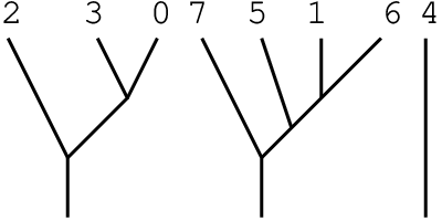
A tree is a leaf-labeled rooted binary tree and a forest is a set of such trees, see Fig. 1. Vertices are either inner vertices (valence 33) or leaves and roots (valence 11). By convention, edges are oriented towards the root. Leaves are bijectively labeled by a finite set. An half-edge is a pair made of an inner vertex and an incident edge (incoming or outcoming). Trees and forests are pictured with their roots down and their leaves up, but are not to be considered as planar.
Refer to caption
Figure 1: A forest on {0,1,2,…,7}.\{0,1,2,\dots,7\}.

1.1 The determinant operad and orientations

An orientation of a finite set XX is a maximal exterior power of the elements of this set, i.e a generator of the ℤ\mathbb{Z}-module Λ|X|​ℤ​X\Lambda^{|X|}\mathbb{Z}X.

Let us recall the definition of the suspended commutative associative operad Det\operatorname{Det} introduced by Ginzburg and Kapranov [3]. Let II be a finite set, then Det⁡(I)\operatorname{Det}(I) is the determinant vector space of ℚ​I\mathbb{Q}I. This vector space is one-dimensional, spanned by the orientations of II (for example 1∧3∧4∧21\wedge 3\wedge 4\wedge 2 in Det⁡({1,2,3,4})\operatorname{Det}(\{1,2,3,4\})) and is placed in degree |I|−1|I|-1. The composition of the operad Det\operatorname{Det} is given by the rule

(x∧⋆)∘⋆y=x∧y,(x\wedge\star)\circ_{\star}y=x\wedge y, (1)

for all x∈Det⁡(I)x\in\operatorname{Det}(I) and y∈Det⁡(J)y\in\operatorname{Det}(J).

It is well known and easy to check that Det\operatorname{Det} has the presentation by the antisymmetric generator ei,j=i∧je_{i,j}=i\wedge j of degree 11 in Det⁡({i,j})\operatorname{Det}(\{i,j\}) satisfying

ei,⋆∘⋆ej,k=ek,⋆∘⋆ei,j.e_{i,\star}\circ_{\star}e_{j,k}=e_{k,\star}\circ_{\star}e_{i,j}. (2)

The operad Det\operatorname{Det} is binary quadratic and Koszul, see [3] for the definitions of these notions.

1.2 The Griess operad and rooted binary trees

The operad Gri\operatorname{Gri} describing commutative but not necessarily associative algebras (sometimes called Griess algebras) admits the following description. The space Gri⁡(I)\operatorname{Gri}(I) has a basis indexed by rooted binary trees with leaves labeled by II and the composition is grafting. This vector space is placed in degree 00. In fact, Gri\operatorname{Gri} is the free operad on a binary symmetric generator ωi,j\omega_{i,j} of degree 00 corresponding to the unique rooted binary tree with two leaves labeled by {i,j}\{i,j\}. The operad Gri\operatorname{Gri} is binary quadratic and Koszul.

1.3 The operad BB of root-oriented forests

For the definition and properties of the notion of distributive law from an operad to another one, see [6].

Proposition 1.1

The following formula defines a distributive law
from Gri∘Det\operatorname{Gri}\circ\operatorname{Det} to Det∘Gri\operatorname{Det}\circ\operatorname{Gri} :

ωi,⋆∘⋆ej,k=ej,⋆∘⋆ωi,k−ek,⋆∘⋆ωi,j.\omega_{i,\star}\circ_{\star}e_{j,k}=e_{j,\star}\circ_{\star}\omega_{i,k}-e_{k,\star}\circ_{\star}\omega_{i,j}. (3)

Proof. As Gri\operatorname{Gri} is a free operad, one has only to check that the rewriting of

ωi,⋆∘⋆(ej,#∘#ek,ℓ)−ωi,⋆∘⋆(ek,#∘#eℓ,j),\omega_{i,\star}\circ_{\star}(e_{j,\#}\circ_{\#}e_{k,\ell})-\omega_{i,\star}\circ_{\star}(e_{k,\#}\circ_{\#}e_{\ell,j}), (4)

using (3) as a replacement rule, gives zero modulo the relation (2) which defines Det\operatorname{Det}. Indeed, one has

ωi,⋆\displaystyle\omega_{i,\star} ∘⋆(ej,#∘#ek,ℓ)=(ωi,⋆∘⋆ej,#)∘#ek,ℓ\displaystyle\circ_{\star}(e_{j,\#}\circ_{\#}e_{k,\ell})=(\omega_{i,\star}\circ_{\star}e_{j,\#})\circ_{\#}e_{k,\ell}
=(ej,⋆∘⋆ωi,#−e#,⋆∘⋆ωi,j)∘#ek,ℓ\displaystyle=(e_{j,\star}\circ_{\star}\omega_{i,\#}-e_{\#,\star}\circ_{\star}\omega_{i,j})\circ_{\#}e_{k,\ell}
=ej,⋆∘⋆(ωi,#∘#ek,ℓ)−(e#,⋆∘⋆ωi,j)∘#ek,ℓ\displaystyle=e_{j,\star}\circ_{\star}(\omega_{i,\#}\circ_{\#}e_{k,\ell})-(e_{\#,\star}\circ_{\star}\omega_{i,j})\circ_{\#}e_{k,\ell}
=ej,⋆∘⋆(ek,#∘#ωi,ℓ−eℓ,#∘#ωi,k)−(e#,⋆∘#ek,ℓ)∘⋆ωi,j\displaystyle=e_{j,\star}\circ_{\star}(e_{k,\#}\circ_{\#}\omega_{i,\ell}-e_{\ell,\#}\circ_{\#}\omega_{i,k})-(e_{\#,\star}\circ_{\#}e_{k,\ell})\circ_{\star}\omega_{i,j}
=(ej,⋆∘⋆ek,#)∘#ωi,ℓ−(ej,⋆∘⋆eℓ,#)∘#ωi,k−(e#,⋆∘#ek,ℓ)∘⋆ωi,j\displaystyle=(e_{j,\star}\circ_{\star}e_{k,\#})\circ_{\#}\omega_{i,\ell}-(e_{j,\star}\circ_{\star}e_{\ell,\#})\circ_{\#}\omega_{i,k}-(e_{\#,\star}\circ_{\#}e_{k,\ell})\circ_{\star}\omega_{i,j}
=(ej,⋆∘⋆ek,#)∘#ωi,ℓ+(ej,⋆∘⋆e#,ℓ)∘#ωi,k+(e#,⋆∘⋆ek,ℓ)∘#ωi,j\displaystyle=(e_{j,\star}\circ_{\star}e_{k,\#})\circ_{\#}\omega_{i,\ell}+(e_{j,\star}\circ_{\star}e_{\#,\ell})\circ_{\#}\omega_{i,k}+(e_{\#,\star}\circ_{\star}e_{k,\ell})\circ_{\#}\omega_{i,j}
=(ej,⋆∘⋆ek,#)∘#ωi,ℓ+(eℓ,⋆∘⋆ej,#)∘#ωi,k+(ek,⋆∘⋆eℓ,#)∘#ωi,j.\displaystyle=(e_{j,\star}\circ_{\star}e_{k,\#})\circ_{\#}\omega_{i,\ell}+(e_{\ell,\star}\circ_{\star}e_{j,\#})\circ_{\#}\omega_{i,k}+(e_{k,\star}\circ_{\star}e_{\ell,\#})\circ_{\#}\omega_{i,j}.

This expression is invariant by cyclic permutation of j,k,ℓj,k,\ell. This shows that the rewriting of (4) is zero, which proves the proposition.  

Let us summarize the description of the operad defined by this distributive law.

Proposition 1.2

The operad BB defined on Det∘Gri\operatorname{Det}\circ\operatorname{Gri} by this distributive law is isomorphic to the quotient of the free operad generated by ei,je_{i,j} antisymmetric in degree 11 and ωi,j\omega_{i,j} symmetric in degree 00 by the following relations.

ei,⋆∘⋆ej,k\displaystyle e_{i,\star}\circ_{\star}e_{j,k} =ek,⋆∘⋆ei,j,\displaystyle=e_{k,\star}\circ_{\star}e_{i,j}, (5)
ωi,⋆∘⋆ej,k\displaystyle\omega_{i,\star}\circ_{\star}e_{j,k} =ej,⋆∘⋆ωi,k−ek,⋆∘⋆ωi,j.\displaystyle=e_{j,\star}\circ_{\star}\omega_{i,k}-e_{k,\star}\circ_{\star}\omega_{i,j}. (6)

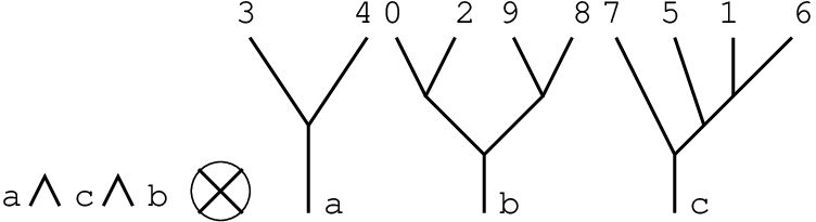
A root-orientation of a forest FF is an orientation of the set of roots of FF. A root-oriented forest is a tensor product of a root-orientation and a forest, see Fig. 2. By the construction of BB by a distributive law, the vector space B⁡(I)B(I) has a basis indexed by root-oriented forests. The degree of a root-oriented forest is the number of roots minus one.
Refer to caption
Figure 2: A root-oriented forest on {0,1,2,…,9}\{0,1,2,\dots,9\}.
Proposition 1.3

The operad BB is binary quadratic and Koszul.

Proof. Koszulness follows from a theorem of Markl [6] since BB is defined by a distributive law between two Koszul operads.  

Here is a description of the composition in the generators. The generator ei,je_{i,j} acts on forests by disjoint union. Let F1⊔F2F_{1}\sqcup F_{2} be the disjoint union of two forests F1F_{1} and F2F_{2}. We use (from now on) the abuse of notation (−1)x(-1)^{x} for (−1)deg⁡(x)(-1)^{\deg(x)} when xx is homogeneous and also (−1)o(-1)^{o} instead of (−1)deg⁡(o)(-1)^{\deg(o)} for any kind of orientation oo. The degree of an orientation is the number of wedge signs that it contains.

Proposition 1.4

Let o1⊗F1o_{1}\otimes F_{1} and o2⊗F2o_{2}\otimes F_{2} be two root-oriented forests. Then

e⋆,#∘⋆(o1⊗F1)∘#(o2⊗F2)=(−1)o1o1∧o2⊗(F1⊔F2).e_{\star,\#}\circ_{\star}(o_{1}\otimes F_{1})\circ_{\#}(o_{2}\otimes F_{2})=(-1)^{o_{1}}o_{1}\wedge o_{2}\otimes(F_{1}\sqcup F_{2}). (7)

Proof. The proposition can be restated as follows. Let x∈B⁡(I)x\in B(I) and y∈B⁡(J)y\in B(J). Then

(e⋆,#∘⋆x)∘#y=(−1)x​x∧y,(e_{\star,\#}\circ_{\star}x)\circ_{\#}y=(-1)^{x}x\wedge y,

Indeed, one has e#,⋆∘⋆x=#∧xe_{\#,\star}\circ_{\star}x=\#\wedge x and (x∧#)∘#y=x∧y(x\wedge\#)\circ_{\#}y=x\wedge y by the composition rule of Det\operatorname{Det}. The sign is given by e#,⋆=−e⋆,#e_{\#,\star}=-e_{\star,\#} and #∧x=(−1)x+1​x∧#\#\wedge x=(-1)^{x+1}x\wedge\#.  

The generator ωi,j\omega_{i,j} acts on trees by grafting. Let T1∨T2T_{1}\vee T_{2} be the tree obtained by grafting T1T_{1} and T2T_{2} on the two leaves of the tree with one inner vertex.

Proposition 1.5

Let o1⊗T1o_{1}\otimes T_{1} and o2⊗T2o_{2}\otimes T_{2} be two root-oriented trees. Then

ω⋆,#∘⋆(o1⊗T1)∘#(o2⊗T2)=o⊗(T1∨T2),\omega_{\star,\#}\circ_{\star}(o_{1}\otimes T_{1})\circ_{\#}(o_{2}\otimes T_{2})=o\otimes(T_{1}\vee T_{2}), (8)

where oo is the unique root-orientation of the tree T1∨T2T_{1}\vee T_{2}.

Proof. This is just the composition of Gri\operatorname{Gri}, restated inside BB, by definition of the composition in an operad defined by a distributive law.  

2 The Bessel operad as a suspension

This section is devoted to the operad Bess=Det⊗B\operatorname{Bess}=\operatorname{Det}\otimes B which is a suspended version of BB. This suspension is necessary for the definition of a Hopf operad structure in the next section.

The generating series of the operad Bess\operatorname{Bess} has for coefficients the Bessel polynomials [4, 5], which are known to count the forests (sets) of rooted leaf-labeled binary trees, hence the chosen name.

2.1 Outer and inner orientations

By its definition, the vector space Bess⁡(I)\operatorname{Bess}(I) has a basis indexed by tensor products o1⊗o2⊗Fo_{1}\otimes o_{2}\otimes F where o1o_{1} is an orientation of II and o2o_{2} is a root-orientation of the forest FF. This tensor product of two orientations is called an outer orientation of FF. In this section, an alternative description is given for this kind of orientation, which will be more convenient later.

A global orientation of a forest FF is an orientation of the set V⁡(F)⊔{RF}V(F)\sqcup\{R_{F}\}, where V⁡(F)V(F) is the set of inner vertices of FF and RFR_{F} is an auxiliary element.

A local orientation of a forest FF at an inner vertex vv is an orientation of its 33 incident half-edges (which is of course equivalent to a cyclic order).

An inner-oriented forest is a tensor product o⊗⨂v∈V⁡(F)ov⊗Fo\otimes\bigotimes_{v\in V(F)}o_{v}\otimes F, where oo is a global orientation of the forest FF and the ovo_{v} are local orientations of FF at its inner vertices. This will from now on be abridged o⊗Fo\otimes F, where oo is a global orientation, the local orientations being implicit. Notice that the order in the product of the local orientations do not matter, as they have degree 22.

One can identify an outer orientation o1⊗o2o_{1}\otimes o_{2} with an inner orientation in the following way.

  1. 1.

    Consider the exterior product o1∧RF∧o2o_{1}\wedge R_{F}\wedge o_{2} where RFR_{F} is an auxiliary element.

  2. 2.

    Remove from this exterior product all possible pairs ℓ∧r\ell\ \wedge r where ℓ\ell is a leaf and rr is a root which are related by an edge.

  3. 3.

    Add to this exterior product pairs e+∧e−e^{+}\wedge e^{-} for all edges ee between two inner vertices. Here e+e^{+} (resp. e−e^{-}) stands for the upper (resp. lower) half-edge.

The result is an exterior product on all half-edges of FF and an auxiliary element RFR_{F}. One can assume that half-edges are gathered by three according to their incident inner vertex. Replacing each such triple ev1∧ev2∧ev3e_{v}^{1}\wedge e_{v}^{2}\wedge e_{v}^{3} by the vertex vv, one gets a global orientation of FF. One has to keep track of what has been replaced. This is done by assigning the local orientation ov=ev1∧ev2∧ev3o_{v}=e_{v}^{1}\wedge e_{v}^{2}\wedge e_{v}^{3} to the inner vertex vv.

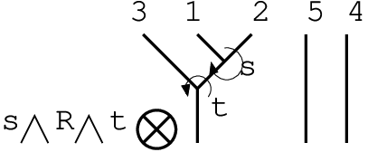
Here is an example of this equivalence of orientations. Consider the outer-oriented forest shown in Fig. 3. One can compute the corresponding inner orientation.

1∧2∧4∧3∧5∧RF∧a∧c∧b\displaystyle 1\wedge 2\wedge 4\wedge 3\wedge 5\wedge R_{F}\wedge a\wedge c\wedge b
=\displaystyle=\quad 1∧2∧3∧5∧RF∧a∧b\displaystyle 1\wedge 2\wedge 3\wedge 5\wedge R_{F}\wedge a\wedge b
=\displaystyle=\quad 1∧2∧3∧RF∧a\displaystyle 1\wedge 2\wedge 3\wedge R_{F}\wedge a
=\displaystyle=\quad 1∧2∧3∧RF∧a∧e+∧e−\displaystyle 1\wedge 2\wedge 3\wedge R_{F}\wedge a\wedge e^{+}\wedge e^{-}
=\displaystyle=\quad (1∧2∧e+)∧RF∧(3∧a∧e−),\displaystyle(1\wedge 2\wedge e^{+})\wedge R_{F}\wedge(3\wedge a\wedge e^{-}),

where e+e^{+} and e−e^{-} are the upper and lower half-edges of the unique inner edge. Hence one can take the global orientation to be s∧RF∧ts\wedge R_{F}\wedge t (where ss is the upper vertex and tt the lower one) and the local orientations to be 1∧2∧e+1\wedge 2\wedge e^{+} at vertex ss and 3∧a∧e−3\wedge a\wedge e^{-} at vertex tt. The result is shown in Fig. 4.

The grading is modified (but its parity is not changed) in order that the forests with no inner vertex are in degree 00, which will be convenient in the next section. From now on, the degree of an inner-oriented forest is the number of its inner vertices.

Refer to caption
Figure 3: An outer-oriented forest on {1,2,3,4,5}\{1,2,3,4,5\}.
Refer to caption
Figure 4: An inner-oriented forest on {1,2,3,4,5}\{1,2,3,4,5\}.

2.2 Presentation of Bess\operatorname{Bess}

From the known presentation of BB, a presentation of Bess\operatorname{Bess} by generators and relations is given in this section.

Let Ei,jE_{i,j} be the inner-oriented forest with two trees on {i,j}\{i,j\} defined by the outer-oriented formula Ei,j=(j∧i)⊗ei,jE_{i,j}=(j\wedge i)\otimes e_{i,j}. It is symmetric of degree 00. As an inner-oriented forest, it is

R⊗|i|j.R\otimes\stackrel{{\scriptstyle i}}{{|}}\,\stackrel{{\scriptstyle j}}{{|}}. (9)

Let Ωi,j\Omega_{i,j} be the inner-oriented tree on {i,j}\{i,j\} defined by the outer-oriented formula Ωi,j=(i∧j)⊗ωi,j\Omega_{i,j}=(i\wedge j)\otimes\omega_{i,j}. It is antisymmetric of degree 11. As an inner-oriented tree, it is given by Fig. 5.

Refer to caption
Figure 5: Ωi,j\Omega_{i,j} as an inner-oriented tree.
Proposition 2.1

The operad Bess\operatorname{Bess} is isomorphic to the quotient of the free operad on the generators Ei,jE_{i,j} symmetric of degree 00 and Ωi,j\Omega_{i,j} antisymmetric of degree 11 by the relations

Ei,⋆∘⋆Ej,k\displaystyle E_{i,\star}\circ_{\star}E_{j,k} =Ek,⋆∘⋆Ei,j,\displaystyle=E_{k,\star}\circ_{\star}E_{i,j}, (10)
Ωi,⋆∘⋆Ej,k\displaystyle\Omega_{i,\star}\circ_{\star}E_{j,k} =Ej,⋆∘⋆Ωi,k+Ek,⋆∘⋆Ωi,j.\displaystyle=E_{j,\star}\circ_{\star}\Omega_{i,k}+E_{k,\star}\circ_{\star}\Omega_{i,j}. (11)

Proof. The tensor product by the operad Det\operatorname{Det} acts essentially by changing all the signs. It is well known that the suspended operad has a presentation by similar generators and relations (up to sign) as it is simply given by a shift of grading at the level of algebras. Let us compute the new relations for our chosen generators. First,

Ei,⋆∘⋆Ej,k\displaystyle E_{i,\star}\circ_{\star}E_{j,k} =((⋆∧i)⊗ei,⋆)∘⋆((k∧j)⊗ej,k)\displaystyle=((\star\wedge i)\otimes e_{i,\star})\circ_{\star}((k\wedge j)\otimes e_{j,k})
=((i∧⋆)∘⋆(k∧j))⊗(ei,⋆∘⋆ej,k)\displaystyle=((i\wedge\star)\circ_{\star}(k\wedge j))\otimes(e_{i,\star}\circ_{\star}e_{j,k})
=(i∧k∧j)⊗(ei,⋆∘⋆ej,k).\displaystyle=(i\wedge k\wedge j)\otimes(e_{i,\star}\circ_{\star}e_{j,k}).

Therefore Ei,⋆∘⋆Ej,kE_{i,\star}\circ_{\star}E_{j,k} is invariant by cyclic permutation of i,j,ki,j,k. One also has

Ωi,⋆∘⋆Ej,k\displaystyle\Omega_{i,\star}\circ_{\star}E_{j,k} =((i∧⋆)⊗ωi,⋆)∘⋆((k∧j)⊗ej,k)\displaystyle=((i\wedge\star)\otimes\omega_{i,\star})\circ_{\star}((k\wedge j)\otimes e_{j,k})
=((i∧⋆)∘⋆(k∧j))⊗(ωi,⋆∘⋆ej,k)\displaystyle=((i\wedge\star)\circ_{\star}(k\wedge j))\otimes(\omega_{i,\star}\circ_{\star}e_{j,k})
=(i∧k∧j)⊗(ej,⋆∘⋆ωi,k−ek,⋆∘⋆ωi,j).\displaystyle=(i\wedge k\wedge j)\otimes(e_{j,\star}\circ_{\star}\omega_{i,k}-e_{k,\star}\circ_{\star}\omega_{i,j}).
OPEN=(j∧i∧k)⊗(ej,⋆∘⋆ωi,k)+(k∧i∧j)⊗(ek,⋆∘⋆ωi,j))\displaystyle=(j\wedge i\wedge k)\otimes(e_{j,\star}\circ_{\star}\omega_{i,k})+(k\wedge i\wedge j)\otimes(e_{k,\star}\circ_{\star}\omega_{i,j}))
=Ej,⋆∘⋆Ωi,k+Ek,⋆∘⋆Ωi,j.\displaystyle=E_{j,\star}\circ_{\star}\Omega_{i,k}+E_{k,\star}\circ_{\star}\Omega_{i,j}.
 

The action of EE is then described as follows.

Proposition 2.2

Let o1⊗F1o_{1}\otimes F_{1} and o2⊗F2o_{2}\otimes F_{2} be two inner-oriented forests. Then

E⋆,#∘⋆(o1⊗F1)∘#(o2⊗F2)=(o1⊔o2)⊗(F1⊔F2),E_{\star,\#}\circ_{\star}(o_{1}\otimes F_{1})\circ_{\#}(o_{2}\otimes F_{2})=(o_{1}\sqcup o_{2})\otimes(F_{1}\sqcup F_{2}), (12)

where the global orientation o1⊔o2o_{1}\sqcup o_{2} is obtained from o1∧r∧o2o_{1}\wedge r\wedge o_{2} by replacing R1∧r∧R2R_{1}\wedge r\wedge R_{2} by RR. The local orientations are unchanged.

Proof. Let o1′⊗o1′′o^{\prime}_{1}\otimes o^{\prime\prime}_{1} and o2′⊗o2′′o^{\prime}_{2}\otimes o^{\prime\prime}_{2} be the corresponding outer orientations of F1F_{1} and F2F_{2}. Using Prop. 1.4, one has

E⋆,#∘⋆(o1⊗F1)∘#(o2⊗F2)=((#∧⋆)⊗e⋆,#)∘⋆(o′1⊗o′′1⊗F1)∘#(o′2⊗o′′2⊗F2)=(−1)o1′+o2′+o2′​o1′′((#∧⋆)∘⋆o′1∘#o′2)⊗(e⋆,#∘⋆(o′′1⊗F1)∘#(o′′2⊗F2))=(−1)(1+o1′′)​(1+o2′)​o1′∧o2′⊗o1′′∧o2′′⊗(F1⊔F2).E_{\star,\#}\circ_{\star}(o_{1}\otimes F_{1})\circ_{\#}(o_{2}\otimes F_{2})=((\#\wedge\star)\otimes e_{\star,\#})\circ_{\star}(o^{\prime}_{1}\otimes o^{\prime\prime}_{1}\otimes F_{1})\circ_{\#}(o^{\prime}_{2}\otimes o^{\prime\prime}_{2}\otimes F_{2})\\ =(-1)^{o^{\prime}_{1}+o^{\prime}_{2}+o^{\prime}_{2}o^{\prime\prime}_{1}}((\#\wedge\star)\circ_{\star}o^{\prime}_{1}\circ_{\#}o^{\prime}_{2})\otimes(e_{\star,\#}\circ_{\star}(o^{\prime\prime}_{1}\otimes F_{1})\circ_{\#}(o^{\prime\prime}_{2}\otimes F_{2}))\\ =(-1)^{(1+o^{\prime\prime}_{1})(1+o^{\prime}_{2})}o^{\prime}_{1}\wedge o^{\prime}_{2}\otimes o^{\prime\prime}_{1}\wedge o^{\prime\prime}_{2}\otimes(F_{1}\sqcup F_{2}).

Hence the corresponding inner orientation is given by

(−1)(1+o1′′)​(1+o2′)​o1′∧o2′∧R∧o1′′∧o2′′.(-1)^{(1+o^{\prime\prime}_{1})(1+o^{\prime}_{2})}o^{\prime}_{1}\wedge o^{\prime}_{2}\wedge R\wedge o^{\prime\prime}_{1}\wedge o^{\prime\prime}_{2}.

On the other hand, let us compute the orientation corresponding to o1⊔o2o_{1}\sqcup o_{2}.

o1′∧R1∧o1′′∧r∧o2′∧R2∧o2′′=(−1)(1+o1′′)​(1+o2′)​o1′∧o2′∧R∧o1′′∧o2′′.o^{\prime}_{1}\wedge R_{1}\wedge o^{\prime\prime}_{1}\wedge r\wedge o^{\prime}_{2}\wedge R_{2}\wedge o^{\prime\prime}_{2}=(-1)^{(1+o^{\prime\prime}_{1})(1+o^{\prime}_{2})}o^{\prime}_{1}\wedge o^{\prime}_{2}\wedge R\wedge o^{\prime\prime}_{1}\wedge o^{\prime\prime}_{2}.

Therefore the two orientations are the same.  

The action of Ω\Omega on trees has the following description.

Proposition 2.3

Let o1⊗T1o_{1}\otimes T_{1} and o2⊗T2o_{2}\otimes T_{2} be two inner-oriented trees. Then

Ω⋆,#∘⋆(o1⊗T1)∘#(o2⊗T2)=(o1∨o2)⊗(T1∨T2),\Omega_{\star,\#}\circ_{\star}(o_{1}\otimes T_{1})\circ_{\#}(o_{2}\otimes T_{2})=(o_{1}\vee o_{2})\otimes(T_{1}\vee T_{2}), (13)

where the global orientation o1∨o2o_{1}\vee o_{2} is defined by (−1)o1​o1∧o2(-1)^{o_{1}}o_{1}\wedge o_{2} modulo R1∧R2=R∧vR_{1}\wedge R_{2}=R\wedge v where vv is the inner vertex of Ω\Omega. The local orientations are unchanged.

Proof. Let o1′⊗root1o^{\prime}_{1}\otimes\operatorname{root}_{1} and o2′⊗root2o^{\prime}_{2}\otimes\operatorname{root}_{2} be the corresponding outer orientations of T1T_{1} and T2T_{2}. Using Prop. 1.5, one has

Ω⋆,#∘⋆(o′1⊗root1⊗T1)∘#(o′2⊗root2⊗T2)=((⋆∧#)∘⋆o′1∘#o′2)⊗(ω⋆,#∘⋆root1⊗T1∘#root2⊗T2)=(−1)o1′(o′1∧o′2)⊗root⊗(T1∨T2).\Omega_{\star,\#}\circ_{\star}(o^{\prime}_{1}\otimes\operatorname{root}_{1}\otimes T_{1})\circ_{\#}(o^{\prime}_{2}\otimes\operatorname{root}_{2}\otimes T_{2})\\ =((\star\wedge\#)\circ_{\star}o^{\prime}_{1}\circ_{\#}o^{\prime}_{2})\otimes(\omega_{\star,\#}\circ_{\star}\operatorname{root}_{1}\otimes T_{1}\circ_{\#}\operatorname{root}_{2}\otimes T_{2})\\ =(-1)^{o^{\prime}_{1}}(o^{\prime}_{1}\wedge o^{\prime}_{2})\otimes\operatorname{root}\otimes(T_{1}\vee T_{2}).

So the corresponding orientation is (−1)o1′​o1′∧o2′∧R∧root(-1)^{o^{\prime}_{1}}o^{\prime}_{1}\wedge o^{\prime}_{2}\wedge R\wedge\operatorname{root}. Introducing pairs of half-edges gives

(−1)o1′​o1′∧o2′∧R∧root∧root1∧e1−∧root2∧e2−,(-1)^{o^{\prime}_{1}}o^{\prime}_{1}\wedge o^{\prime}_{2}\wedge R\wedge\operatorname{root}\wedge\operatorname{root}_{1}\wedge e_{1}^{-}\wedge\operatorname{root}_{2}\wedge e_{2}^{-},

where e1−e_{1}^{-} and e2−e_{2}^{-} are lower half-edges. This is equivalent with the local orientation (root∧e1−∧e2−)(\operatorname{root}\wedge e_{1}^{-}\wedge e_{2}^{-}) at vertex vv (which is the local orientation of Ω\Omega, see figure 5) and orientation

(−1)o1′​o1′∧o2′∧R∧root1∧v∧root2.(-1)^{o^{\prime}_{1}}o^{\prime}_{1}\wedge o^{\prime}_{2}\wedge R\wedge\operatorname{root}_{1}\wedge v\wedge\operatorname{root}_{2}.

On the other hand, the proposed orientation is

(−1)o1​o1′∧R1∧root1∧o2′∧R2∧root2=(−1)o1​o1′∧o2′∧R1∧root1∧R2∧root2.(-1)^{o_{1}}o^{\prime}_{1}\wedge R_{1}\wedge\operatorname{root}_{1}\wedge o^{\prime}_{2}\wedge R_{2}\wedge\operatorname{root}_{2}=(-1)^{o_{1}}o^{\prime}_{1}\wedge o^{\prime}_{2}\wedge R_{1}\wedge\operatorname{root}_{1}\wedge R_{2}\wedge\operatorname{root}_{2}.

This matches the computed orientation, as R1∧R2=R∧vR_{1}\wedge R_{2}=R\wedge v and (−1)o1=(−1)o1′(-1)^{o_{1}}=(-1)^{o^{\prime}_{1}}.  

Let us extend the definition of ∨\vee from trees to forests, as follows. Let F1=T11⊔T12⊔⋯⊔T1mF_{1}=T^{1}_{1}\sqcup T^{2}_{1}\sqcup\dots\sqcup T^{m}_{1} and F2=T21⊔T22⊔⋯⊔T2nF_{2}=T^{1}_{2}\sqcup T^{2}_{2}\sqcup\dots\sqcup T^{n}_{2} be forests, where the TT are trees. Define F1∨F2F_{1}\vee F_{2} to be the sum

∑1≤a≤m∑1≤b≤n(T1a∨T2b)⊔T11⊔⋯⊔T^1a⊔⋯⊔T22⊔⋯⊔T^2b⊔…,\sum_{1\leq a\leq m}\sum_{1\leq b\leq n}(T^{a}_{1}\vee T^{b}_{2})\sqcup T_{1}^{1}\sqcup\dots\sqcup\widehat{T}^{a}_{1}\sqcup\dots\sqcup T^{2}_{2}\sqcup\dots\sqcup\widehat{T}^{b}_{2}\sqcup\dots,

where T^\widehat{T} means that this term is absent. In words, F1∨F2F_{1}\vee F_{2} is the sum over all possible pairings of a tree from T1T_{1} and a tree from T2T_{2}, where these two trees are replaced in the disjoint union F1⊔F2F_{1}\sqcup F_{2} by their ∨\vee product.

Then Prop. 2.3 is still true for forests instead of just trees, with the extended definition just given for ∨\vee.

Proposition 2.4

Let o1⊗F1o_{1}\otimes F_{1} and o2⊗F2o_{2}\otimes F_{2} be two inner-oriented forests. Then

Ω⋆,#∘⋆(o1⊗F1)∘#(o2⊗F2)=(o1∨o2)⊗(F1∨F2),\Omega_{\star,\#}\circ_{\star}(o_{1}\otimes F_{1})\circ_{\#}(o_{2}\otimes F_{2})=(o_{1}\vee o_{2})\otimes(F_{1}\vee F_{2}), (14)

where the global orientation o1∨o2o_{1}\vee o_{2} is defined by (−1)o1​o1∧o2(-1)^{o_{1}}o_{1}\wedge o_{2} modulo R1∧R2=R∧vR_{1}\wedge R_{2}=R\wedge v where vv is the inner vertex of Ω\Omega. The local orientations are unchanged.

Proof. By recursion on the total number of trees in F1F_{1} and F2F_{2}. The proposition is true if F1F_{1} and F2F_{2} are trees. Let us assume that F2F_{2} has at least two trees.

One the one hand,

Ω⋆,#∘⋆(o1⊗F1)∘#((o2⊔o3)⊗(F2⊔F3))=Ω⋆,#∘⋆(o1⊗F1)∘#(EΔ,∞∘Δ(o2⊗F2)∘∞(o3⊗F3))=Ω⋆,#∘#EΔ,∞∘⋆(o1⊗F1)∘Δ(o2⊗F2)∘∞(o3⊗F3)=(EΔ,#∘#Ω⋆,∞+E∞,#∘#Ω⋆,Δ)∘⋆(o1⊗F1)∘Δ(o2⊗F2)∘∞(o3⊗F3)=(−1)o2​o3EΔ,#∘#Ω⋆,∞∘⋆(o1⊗F1)∘∞(o3⊗F3)∘Δ(o2⊗F2)+E∞,#∘#Ω⋆,Δ∘⋆(o1⊗F1)∘Δ(o2⊗F2)∘∞(o3⊗F3)=(−1)o2​o3EΔ,#∘#((o1∨o3)⊗(F1∨F3))∘Δ(o2⊗F2)+E∞,#∘#((o1∨o2)⊗(F1∨F2))∘∞(o3⊗F3)=(−1)o2​o3​((o1∨o3)⊔o2)⊗((F1∨F3)⊔F2)+((o1∨o2)⊔o3)⊗((F1∨F2)⊔F3).\Omega_{\star,\#}\circ_{\star}(o_{1}\otimes F_{1})\circ_{\#}((o_{2}\sqcup o_{3})\otimes(F_{2}\sqcup F_{3}))\\ =\Omega_{\star,\#}\circ_{\star}(o_{1}\otimes F_{1})\circ_{\#}(E_{\Delta,\infty}\circ_{\Delta}(o_{2}\otimes F_{2})\circ_{\infty}(o_{3}\otimes F_{3}))\\ =\Omega_{\star,\#}\circ_{\#}E_{\Delta,\infty}\circ_{\star}(o_{1}\otimes F_{1})\circ_{\Delta}(o_{2}\otimes F_{2})\circ_{\infty}(o_{3}\otimes F_{3})\\ =(E_{\Delta,\#}\circ_{\#}\Omega_{\star,\infty}+E_{\infty,\#}\circ_{\#}\Omega_{\star,\Delta})\circ_{\star}(o_{1}\otimes F_{1})\circ_{\Delta}(o_{2}\otimes F_{2})\circ_{\infty}(o_{3}\otimes F_{3})\\ =(-1)^{o_{2}o_{3}}E_{\Delta,\#}\circ_{\#}\Omega_{\star,\infty}\circ_{\star}(o_{1}\otimes F_{1})\circ_{\infty}(o_{3}\otimes F_{3})\circ_{\Delta}(o_{2}\otimes F_{2})\\ +E_{\infty,\#}\circ_{\#}\Omega_{\star,\Delta}\circ_{\star}(o_{1}\otimes F_{1})\circ_{\Delta}(o_{2}\otimes F_{2})\circ_{\infty}(o_{3}\otimes F_{3})\\ =(-1)^{o_{2}o_{3}}E_{\Delta,\#}\circ_{\#}((o_{1}\vee o_{3})\otimes(F_{1}\vee F_{3}))\circ_{\Delta}(o_{2}\otimes F_{2})\\ +E_{\infty,\#}\circ_{\#}((o_{1}\vee o_{2})\otimes(F_{1}\vee F_{2}))\circ_{\infty}(o_{3}\otimes F_{3})\\ =(-1)^{o_{2}o_{3}}((o_{1}\vee o_{3})\sqcup o_{2})\otimes((F_{1}\vee F_{3})\sqcup F_{2})+((o_{1}\vee o_{2})\sqcup o_{3})\otimes((F_{1}\vee F_{2})\sqcup F_{3}).

On the other hand, the definition of ∨\vee implies that

(o1∨(o2⊔o3))⊗(F1∨(F2⊔F3))OPEN=(o1∨(o2⊔o3))⊗((F1∨F3)⊔F2)+(o1∨(o2⊔o3))⊗((F1∨F2)⊔F3)).(o_{1}\vee(o_{2}\sqcup o_{3}))\otimes(F_{1}\vee(F_{2}\sqcup F_{3}))\\ =(o_{1}\vee(o_{2}\sqcup o_{3}))\otimes((F_{1}\vee F_{3})\sqcup F_{2})+(o_{1}\vee(o_{2}\sqcup o_{3}))\otimes((F_{1}\vee F_{2})\sqcup F_{3})).

So it remains to compare the orientations. Using their defining properties, it is easy to see that

(−1)o2​o3​(o1∨o3)⊔o2=o1∨(o2⊔o3)=(o1∨o2)⊔o3.(-1)^{o_{2}o_{3}}(o_{1}\vee o_{3})\sqcup o_{2}=o_{1}\vee(o_{2}\sqcup o_{3})=(o_{1}\vee o_{2})\sqcup o_{3}.

The proposition is proved.  

3 A coproduct on Bess\operatorname{Bess}

In this section, a map from Bess\operatorname{Bess} to Bess⊗Bess\operatorname{Bess}\otimes\operatorname{Bess} is first defined on generators, then shown to be given by an explicit formula.

3.1 Definition on generators

Let us define a coproduct Δ:Bess→Bess⊗Bess\Delta:\operatorname{Bess}\to\operatorname{Bess}\otimes\operatorname{Bess} on the generators Ei,jE_{i,j} and Ωi,j\Omega_{i,j} of Bess\operatorname{Bess} by

Δ⁡(Ei,j)\displaystyle\Delta(E_{i,j}) =Ei,j⊗Ei,j,\displaystyle=E_{i,j}\otimes E_{i,j}, (15)
Δ⁡(Ωi,j)\displaystyle\Delta(\Omega_{i,j}) =Ei,j⊗Ωi,j+Ωi,j⊗Ei,j.\displaystyle=E_{i,j}\otimes\Omega_{i,j}+\Omega_{i,j}\otimes E_{i,j}. (16)
Proposition 3.1

These formulas define a coassociative cocommutative morphism of operad from Bess\operatorname{Bess} to Bess⊗Bess\operatorname{Bess}\otimes\operatorname{Bess}, i.e. the structure of a Hopf operad on Bess\operatorname{Bess}. In particular, each Bess⁡(I)\operatorname{Bess}(I) inherits a structure of cocommutative coalgebra.

Proof. Coassociativity and cocommutativity are clear on generators. One has to check that the relations (10) and (11) of Bess\operatorname{Bess} are annihilated by Δ\Delta. First,

Δ⁡(Ei,⋆∘⋆Ej,k)=(Ei,⋆⊗Ei,⋆)∘⋆(Ej,k⊗Ej,k)=(Ei,⋆∘⋆Ej,k)⊗(Ei,⋆∘⋆Ej,k),\Delta(E_{i,\star}\circ_{\star}E_{j,k})=(E_{i,\star}\otimes E_{i,\star})\circ_{\star}(E_{j,k}\otimes E_{j,k})=(E_{i,\star}\circ_{\star}E_{j,k})\otimes(E_{i,\star}\circ_{\star}E_{j,k}),

which inherits the invariance of Ei,⋆∘⋆Ej,kE_{i,\star}\circ_{\star}E_{j,k} under cyclic permutations of i,j,ki,j,k. Hence Δ\Delta vanishes on the relation (10). For the other relation, on the one hand

Δ\displaystyle\Delta (Ωi,⋆∘⋆Ej,k)=(Ei,⋆⊗Ωi,⋆+Ωi,⋆⊗Ei,⋆)∘⋆(Ej,k⊗Ej,k)\displaystyle(\Omega_{i,\star}\circ_{\star}E_{j,k})=(E_{i,\star}\otimes\Omega_{i,\star}+\Omega_{i,\star}\otimes E_{i,\star})\circ_{\star}(E_{j,k}\otimes E_{j,k})
=(Ei,⋆⊗Ωi,⋆)∘⋆(Ej,k⊗Ej,k)+(Ωi,⋆⊗Ei,⋆)∘⋆(Ej,k⊗Ej,k)\displaystyle=(E_{i,\star}\otimes\Omega_{i,\star})\circ_{\star}(E_{j,k}\otimes E_{j,k})+(\Omega_{i,\star}\otimes E_{i,\star})\circ_{\star}(E_{j,k}\otimes E_{j,k})
=(Ei,⋆∘⋆Ej,k)⊗(Ωi,⋆∘⋆Ej,k)+(Ωi,⋆∘⋆Ej,k)⊗(Ei,⋆∘⋆Ej,k)\displaystyle=(E_{i,\star}\circ_{\star}E_{j,k})\otimes(\Omega_{i,\star}\circ_{\star}E_{j,k})+(\Omega_{i,\star}\circ_{\star}E_{j,k})\otimes(E_{i,\star}\circ_{\star}E_{j,k})
=(Ei,⋆∘⋆Ej,k)⊗(Ej,⋆∘⋆Ωi,k)+(Ei,⋆∘⋆Ej,k)⊗(Ek,⋆∘⋆Ωi,j)\displaystyle=(E_{i,\star}\circ_{\star}E_{j,k})\otimes(E_{j,\star}\circ_{\star}\Omega_{i,k})+(E_{i,\star}\circ_{\star}E_{j,k})\otimes(E_{k,\star}\circ_{\star}\Omega_{i,j})
+(Ej,⋆∘⋆Ωi,k)⊗(Ei,⋆∘⋆Ej,k)+(Ek,⋆∘⋆Ωi,j)⊗(Ei,⋆∘⋆Ej,k).\displaystyle+(E_{j,\star}\circ_{\star}\Omega_{i,k})\otimes(E_{i,\star}\circ_{\star}E_{j,k})+(E_{k,\star}\circ_{\star}\Omega_{i,j})\otimes(E_{i,\star}\circ_{\star}E_{j,k}).

On the other hand,

Δ\displaystyle\Delta (Ej,⋆∘⋆Ωi,k)=(Ej,⋆⊗Ej,⋆)∘⋆(Ei,k⊗Ωi,k+Ωi,k⊗Ei,k)\displaystyle(E_{j,\star}\circ_{\star}\Omega_{i,k})=(E_{j,\star}\otimes E_{j,\star})\circ_{\star}(E_{i,k}\otimes\Omega_{i,k}+\Omega_{i,k}\otimes E_{i,k})
=(Ej,⋆∘⋆Ei,k)⊗(Ej,⋆∘⋆Ωi,k)+(Ej,⋆∘⋆Ωi,k)⊗(Ej,⋆∘⋆Ei,k)\displaystyle=(E_{j,\star}\circ_{\star}E_{i,k})\otimes(E_{j,\star}\circ_{\star}\Omega_{i,k})+(E_{j,\star}\circ_{\star}\Omega_{i,k})\otimes(E_{j,\star}\circ_{\star}E_{i,k})
=(Ei,⋆∘⋆Ej,k)⊗(Ej,⋆∘⋆Ωi,k)+(Ej,⋆∘⋆Ωi,k)⊗(Ei,⋆∘⋆Ej,k),\displaystyle=(E_{i,\star}\circ_{\star}E_{j,k})\otimes(E_{j,\star}\circ_{\star}\Omega_{i,k})+(E_{j,\star}\circ_{\star}\Omega_{i,k})\otimes(E_{i,\star}\circ_{\star}E_{j,k}),

and a similar formula holds for Δ⁡(Ek,⋆∘⋆Ωi,j)\Delta(E_{k,\star}\circ_{\star}\Omega_{i,j}). From these formulas, it is clear that Δ\Delta vanishes on relation (11). This proves the proposition.  

3.2 A poset on forests

There is an explicit formula for the coproduct, which is a sum over subsets of the set of inner vertices. A poset on forests involved in this formula is described first.

A leaf is an ancestor of a vertex if there is path from the leaf to the root going through the vertex.

Let FF and F′F^{\prime} be two forests on the set II. Then F′≤FF^{\prime}\leq F if there is a topological map from F′F^{\prime} to FF with the following properties :

  1. 1.

    It is increasing with respect to orientation towards the root.

  2. 2.

    It maps inner vertices to inner vertices injectively.

  3. 3.

    It restricts to the identity on leaves.

In fact, such a topological map from F′F^{\prime} to FF is determined by the image of inner vertices of F′F^{\prime}. Indeed one can recover the map by joining the image of an inner vertex with its ancestor leaves in F′F^{\prime}.

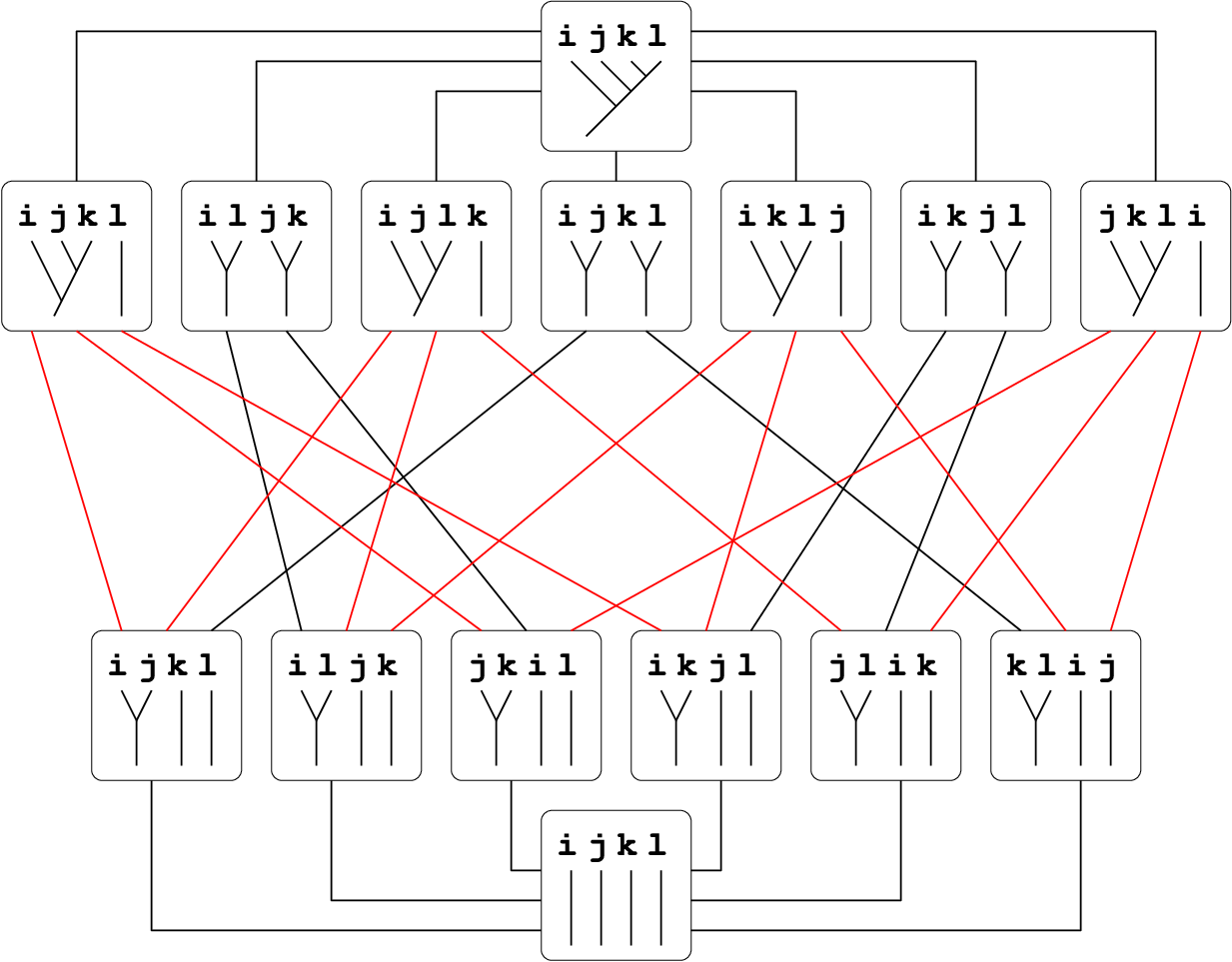
This relation defines a partial order on the set of forests on II. The maximal elements of this poset are the trees. This poset is ranked by the number of inner vertices. Fig. 6 displays an interval in the poset of forests on the set {i,j,k,ℓ}\{i,j,k,\ell\}.

Remark : As can be seen on Fig. 6, the interval in this poset between the minimal element and one of the “comb” trees (which have a leaf with all the inner vertices belonging to its path to the root) can be identified to the partition lattice. The proof is by identifying a forest with the partition of the set of leaves defined by its trees. Details will be given elsewhere.
Refer to caption
Figure 6: An interval in the poset of forests on {i,j,k,ℓ}\{i,j,k,\ell\}.

If FF is a forest on the set II and VV is a subset of the set V⁡(F)V(F) of inner vertices of FF, let γ⁡(F,V)\gamma(F,V) be the sum of forests F′F^{\prime} such that F′≤FF^{\prime}\leq F and the inner vertices of F′F^{\prime} are identified with the elements of VV. The sum γ⁡(V,F)\gamma(V,F), which is an element of the free ℤ\mathbb{Z}-module generated by the set of forests on the finite set II, can also be considered as a set, as it has no multiplicity. Indeed, there is at most one way to complete a injection of inner vertices into a topological map from a given forest F′F^{\prime} to a given forest FF.

Lemma 3.2

Let ⊔\sqcup and ∨\vee be the bilinear extensions of the operations ⊔\sqcup and ∨\vee on forests.

  1. 1.

    Let T=T1∨T2T=T_{1}\vee T_{2} be a tree and V′={v}⊔V1′⊔V2′V^{\prime}=\{v\}\sqcup V^{\prime}_{1}\sqcup V^{\prime}_{2} be a subset of V⁡(T)V(T) containing the bottom vertex vv. Then γ⁡(T,V′)=γ⁡(T1,V1′)∨γ⁡(T2,V2′)\gamma(T,V^{\prime})=\gamma(T_{1},V^{\prime}_{1})\vee\gamma(T_{2},V^{\prime}_{2}).

  2. 2.

    Let T=T1∨T2T=T_{1}\vee T_{2} be a tree and V′=V1′⊔V2′V^{\prime}=V^{\prime}_{1}\sqcup V^{\prime}_{2} be a subset of V⁡(T)V(T) not containing the bottom vertex vv. Then γ⁡(T,V′)=γ⁡(T1,V1′)⊔γ⁡(T2,V2′)\gamma(T,V^{\prime})=\gamma(T_{1},V^{\prime}_{1})\sqcup\gamma(T_{2},V^{\prime}_{2}).

  3. 3.

    Let F=F1⊔F2F=F_{1}\sqcup F_{2} be a forest and V′=V1′⊔V2′V^{\prime}=V^{\prime}_{1}\sqcup V^{\prime}_{2} be a subset of V⁡(F)V(F). Then γ⁡(F,V′)=γ⁡(F1,V1′)⊔γ⁡(F2,V2′)\gamma(F,V^{\prime})=\gamma(F_{1},V^{\prime}_{1})\sqcup\gamma(F_{2},V^{\prime}_{2}).

Proof. The second and third cases are essentially the same and easy consequences of the definition of the poset. If two sets V1V_{1}, V2V_{2} of inner vertices of a forest FF have no ancestor leaf in common, then the set γ⁡(F,V1⊔V2)\gamma(F,V_{1}\sqcup V_{2}) is in bijection with the product γ⁡(F,V1)×γ⁡(F,V2)\gamma(F,V_{1})\times\gamma(F,V_{2}). For γ\gamma seen as a sum, this gives the expected result.

The first case now. Any element of γ⁡(T,V′)\gamma(T,V^{\prime}) is a forest FF with inner vertices V′V^{\prime}. This forest can be restricted to V1′V^{\prime}_{1} and to V2′V^{\prime}_{2} to give two forests F1F_{1} and F2F_{2}. To be able to recover the forest FF from F1F_{1} and F1F_{1}, it is necessary and sufficient to know to which tree of F1F_{1} and to which tree of F2F_{2} the vertex vv was connected in FF. Therefore the set γ⁡(T,V′)\gamma(T,V^{\prime}) is in bijection with the set of quadruples (F1,α,F2,β)(F_{1},\alpha,F_{2},\beta) where F1F_{1} and F2F_{2} are in γ⁡(T1,V1′)\gamma(T_{1},V^{\prime}_{1}) and γ⁡(T2,V2′)\gamma(T_{2},V^{\prime}_{2}), α\alpha is a tree of F1F_{1} and β\beta is a tree of F2F_{2}.

Therefore, seen as a sum, γ⁡(T,V′)\gamma(T,V^{\prime}) is exactly given by the bilinear extension of the operation ∨\vee on forests, which is a sum over the set of pairs of subtrees.  

3.3 Explicit formula for the coproduct

Proposition 3.3

Let o⊗Fo\otimes F be an inner-oriented forest. Then

Δ⁡(o⊗F)=∑V⁡(F)=V′⊔V′′(o′⊗γ⁡(F,V′))⊗(o′′⊗γ⁡(F,V′′)).\Delta(o\otimes F)=\sum_{V(F)=V^{\prime}\sqcup V^{\prime\prime}}\big(o^{\prime}\otimes\gamma(F,V^{\prime})\big)\otimes\big(o^{\prime\prime}\otimes\gamma(F,V^{\prime\prime})\big). (17)

where the local orientations are unchanged and the global orientations satisfy o′∧r∧o′′=oo^{\prime}\wedge r\wedge o^{\prime\prime}=o modulo R′∧r∧R′′=RR^{\prime}\wedge r\wedge R^{\prime\prime}=R.

Proof. The proof is a recursion on the number of inner vertices. The proposition is clear for trees with no inner vertex. The proof of the recursion step is done separately for trees and for forests with at least two trees.

The case of trees

Let o1⊗T1o_{1}\otimes T_{1} and o2⊗T2o_{2}\otimes T_{2} be two inner-oriented trees and let o⊗T=(o1∨o2)⊗(T1∨T2)o\otimes T=(o_{1}\vee o_{2})\otimes(T_{1}\vee T_{2}). Then

Δ(o⊗T)=Δ(Ω⋆,#∘⋆(o1⊗T1)∘#(o2⊗T2))=∑V⁡(T1)=V1′⊔V1′′∑V⁡(T2)=V2′⊔V2′′(Ω⋆,#⊗E⋆,#+E⋆,#⊗Ω⋆,#)∘⋆(o′1⊗γ′1⊗o′′1⊗γ′′1)∘#(o′2⊗γ′2⊗o′′2⊗γ′′2),\Delta(o\otimes T)=\Delta\big(\Omega_{\star,\#}\circ_{\star}(o_{1}\otimes T_{1})\circ_{\#}(o_{2}\otimes T_{2})\big)\\ =\sum_{V(T_{1})=V^{\prime}_{1}\sqcup V^{\prime\prime}_{1}}\sum_{V(T_{2})=V^{\prime}_{2}\sqcup V^{\prime\prime}_{2}}(\Omega_{\star,\#}\otimes E_{\star,\#}+E_{\star,\#}\otimes\Omega_{\star,\#})\\ \circ_{\star}(o^{\prime}_{1}\otimes\gamma^{\prime}_{1}\otimes o^{\prime\prime}_{1}\otimes\gamma^{\prime\prime}_{1})\circ_{\#}(o^{\prime}_{2}\otimes\gamma^{\prime}_{2}\otimes o^{\prime\prime}_{2}\otimes\gamma^{\prime\prime}_{2}), (18)

where γi∗\gamma^{*}_{i} stands for γ⁡(Ti,Vi∗)\gamma(T_{i},V^{*}_{i}).

The first half of this formula corresponding to the expansion of the composition in Ω⋆,#⊗E⋆,#\Omega_{\star,\#}\otimes E_{\star,\#} is given by

∑V⁡(T1)=V1′⊔V1′′∑V⁡(T2)=V2′⊔V2′′(−1)o2′​o1′′(Ω⋆,#∘⋆(o′1⊗γ′1)∘#(o′2⊗γ′2))⊗(E⋆,#∘⋆(o′′1⊗γ′′1)∘#(o′′2⊗γ′′2))=∑V⁡(T1)=V1′⊔V1′′∑V⁡(T2)=V2′⊔V2′′(−1)o2′​o1′′​o¯′⊗(γ1′∨γ2′)⊗o¯′′⊗(γ1′′⊔γ2′′),\sum_{V(T_{1})=V^{\prime}_{1}\sqcup V^{\prime\prime}_{1}}\sum_{V(T_{2})=V^{\prime}_{2}\sqcup V^{\prime\prime}_{2}}(-1)^{o^{\prime}_{2}o^{\prime\prime}_{1}}\\ (\Omega_{\star,\#}\circ_{\star}(o^{\prime}_{1}\otimes\gamma^{\prime}_{1})\circ_{\#}(o^{\prime}_{2}\otimes\gamma^{\prime}_{2}))\otimes(E_{\star,\#}\circ_{\star}(o^{\prime\prime}_{1}\otimes\gamma^{\prime\prime}_{1})\circ_{\#}(o^{\prime\prime}_{2}\otimes\gamma^{\prime\prime}_{2}))\\ =\sum_{V(T_{1})=V^{\prime}_{1}\sqcup V^{\prime\prime}_{1}}\sum_{V(T_{2})=V^{\prime}_{2}\sqcup V^{\prime\prime}_{2}}(-1)^{o^{\prime}_{2}o^{\prime\prime}_{1}}\bar{o}^{\prime}\otimes(\gamma^{\prime}_{1}\vee\gamma^{\prime}_{2})\otimes\bar{o}^{\prime\prime}\otimes(\gamma^{\prime\prime}_{1}\sqcup\gamma^{\prime\prime}_{2}), (19)

the orientations satisfying

o1′∧r1∧o1′′\displaystyle o^{\prime}_{1}\wedge r_{1}\wedge o^{\prime\prime}_{1} =o1\displaystyle=o_{1}\qquad R1′∧r1∧R1′′\displaystyle R^{\prime}_{1}\wedge r_{1}\wedge R^{\prime\prime}_{1} =R1\displaystyle=R_{1}
o2′∧r2∧o2′′\displaystyle o^{\prime}_{2}\wedge r_{2}\wedge o^{\prime\prime}_{2} =o2\displaystyle=o_{2}\qquad R2′∧r2∧R2′′\displaystyle R^{\prime}_{2}\wedge r_{2}\wedge R^{\prime\prime}_{2} =R2\displaystyle=R_{2}
(−1)o1′​o1′∧o2′\displaystyle(-1)^{o^{\prime}_{1}}o^{\prime}_{1}\wedge o^{\prime}_{2} =o¯′\displaystyle=\bar{o}^{\prime}\qquad R′∧s\displaystyle R^{\prime}\wedge s =R1′∧R2′\displaystyle=R^{\prime}_{1}\wedge R^{\prime}_{2}
o1′′∧r′′∧o2′′\displaystyle o^{\prime\prime}_{1}\wedge r^{\prime\prime}\wedge o^{\prime\prime}_{2} =o¯′′\displaystyle=\bar{o}^{\prime\prime}\qquad R1′′∧r′′∧R2′′\displaystyle R^{\prime\prime}_{1}\wedge r^{\prime\prime}\wedge R^{\prime\prime}_{2} =R′′.\displaystyle=R^{\prime\prime}.

On the other hand, one has to compute

∑V⁡(T)=V′⊔V′′v∈V′o′⊗γ⁡(T,V′)⊗o′′⊗γ⁡(T,V′′).\sum_{{V(T)=V^{\prime}\sqcup V^{\prime\prime}}\atop{v\in V^{\prime}}}o^{\prime}\otimes\gamma(T,V^{\prime})\otimes o^{\prime\prime}\otimes\gamma(T,V^{\prime\prime}). (20)

As V⁡(T)={v}⊔V⁡(T1)⊔V⁡(T2)V(T)=\{v\}\sqcup V(T_{1})\sqcup V(T_{2}), one can replace the sum by a double sum, using Lemma 3.2 :

∑V⁡(T1)=V1′⊔V1′′∑V⁡(T2)=V2′⊔V2′′o′⊗(γ1′∨γ2′)⊗o′′⊗(γ1′′⊔γ2′′),\sum_{V(T_{1})=V^{\prime}_{1}\sqcup V^{\prime\prime}_{1}}\sum_{V(T_{2})=V^{\prime}_{2}\sqcup V^{\prime\prime}_{2}}o^{\prime}\otimes(\gamma^{\prime}_{1}\vee\gamma^{\prime}_{2})\otimes o^{\prime\prime}\otimes(\gamma^{\prime\prime}_{1}\sqcup\gamma^{\prime\prime}_{2}),

with the orientations determined by

o′∧r∧o′′\displaystyle o^{\prime}\wedge r\wedge o^{\prime\prime} =o1∨o2\displaystyle=o_{1}\vee o_{2}\qquad R′∧r∧R′′\displaystyle R^{\prime}\wedge r\wedge R^{\prime\prime} =R\displaystyle=R
(−1)o1​o1∧o2\displaystyle(-1)^{o_{1}}o_{1}\wedge o_{2} =o1∨o2\displaystyle=o_{1}\vee o_{2}\qquad R1∧R2\displaystyle R_{1}\wedge R_{2} =R∧s.\displaystyle=R\wedge s.

All these conditions on orientations together imply that the orientations o′⊗o′′o^{\prime}\otimes o^{\prime\prime} and (−1)o2′​o1′′​o′¯⊗o¯′′(-1)^{o^{\prime}_{2}o^{\prime\prime}_{1}}\bar{o^{\prime}}\otimes\bar{o}^{\prime\prime} are the same. Therefore (19) and (20) are equal.

The other half of the sum (18), corresponding to the expansion of the composition in E⋆,#⊗Ω⋆,#E_{\star,\#}\otimes\Omega_{\star,\#}, is shown in the same way to be equal to

∑V⁡(T)=V′⊔V′′v∈V′′o′⊗γ⁡(T,V′)⊗o′′⊗γ⁡(T,V′′).\sum_{V(T)=V^{\prime}\sqcup V^{\prime\prime}\atop{v\in V^{\prime\prime}}}o^{\prime}\otimes\gamma(T,V^{\prime})\otimes o^{\prime\prime}\otimes\gamma(T,V^{\prime\prime}). (21)

Therefore the full sum (18) is given by the expected formula (17) and the recursion step is done for trees.

The case of true forests

Let o1⊗F1o_{1}\otimes F_{1} and o2⊗F2o_{2}\otimes F_{2} be two inner-oriented forests and let o⊗F=(o1⊔o2)⊗(F1⊔F2)o\otimes F=(o_{1}\sqcup o_{2})\otimes(F_{1}\sqcup F_{2}). One has

Δ(o⊗F)=Δ(E⋆,#∘⋆o1⊗F1∘#o2⊗F2)=∑V1=V1′⊔V1′′∑V2=V2′⊔V2′′(E⋆,#⊗E⋆,#)∘⋆(o′1⊗γ′1⊗o′′1⊗γ′′1)∘#(o′2⊗γ′2⊗o′′2⊗γ′′2)=∑V1=V1′⊔V1′′∑V2=V2′⊔V2′′(−1)o2′​o1′′(E⋆,#∘⋆o′1⊗γ′1∘#o′2⊗γ′2)⊗(E⋆,#∘⋆o′′1⊗γ′′1∘#o′′2⊗γ′′2)=∑V1=V1′⊔V1′′∑V2=V2′⊔V2′′(−1)o2′​o1′′​o¯′⊗(γ1′⊔γ2′)⊗o¯′′⊗(γ1′′⊔γ2′′),\Delta(o\otimes F)=\Delta(E_{\star,\#}\circ_{\star}o_{1}\otimes F_{1}\circ_{\#}o_{2}\otimes F_{2})\\ =\sum_{V_{1}=V^{\prime}_{1}\sqcup V^{\prime\prime}_{1}}\sum_{V_{2}=V^{\prime}_{2}\sqcup V^{\prime\prime}_{2}}(E_{\star,\#}\otimes E_{\star,\#})\circ_{\star}(o^{\prime}_{1}\otimes\gamma^{\prime}_{1}\otimes o^{\prime\prime}_{1}\otimes\gamma^{\prime\prime}_{1})\circ_{\#}(o^{\prime}_{2}\otimes\gamma^{\prime}_{2}\otimes o^{\prime\prime}_{2}\otimes\gamma^{\prime\prime}_{2})\\ =\sum_{V_{1}=V^{\prime}_{1}\sqcup V^{\prime\prime}_{1}}\sum_{V_{2}=V^{\prime}_{2}\sqcup V^{\prime\prime}_{2}}(-1)^{o^{\prime}_{2}o^{\prime\prime}_{1}}(E_{\star,\#}\circ_{\star}o^{\prime}_{1}\otimes\gamma^{\prime}_{1}\circ_{\#}o^{\prime}_{2}\otimes\gamma^{\prime}_{2})\otimes(E_{\star,\#}\circ_{\star}o^{\prime\prime}_{1}\otimes\gamma^{\prime\prime}_{1}\circ_{\#}o^{\prime\prime}_{2}\otimes\gamma^{\prime\prime}_{2})\\ =\sum_{V_{1}=V^{\prime}_{1}\sqcup V^{\prime\prime}_{1}}\sum_{V_{2}=V^{\prime}_{2}\sqcup V^{\prime\prime}_{2}}(-1)^{o^{\prime}_{2}o^{\prime\prime}_{1}}\bar{o}^{\prime}\otimes(\gamma^{\prime}_{1}\sqcup\gamma^{\prime}_{2})\otimes\bar{o}^{\prime\prime}\otimes(\gamma^{\prime\prime}_{1}\sqcup\gamma^{\prime\prime}_{2}), (22)

where γi∗\gamma^{*}_{i} stands for γ⁡(Fi,Vi∗)\gamma(F_{i},V^{*}_{i}) and the orientations satisfy

o1′∧r1∧o1′′\displaystyle o^{\prime}_{1}\wedge r_{1}\wedge o^{\prime\prime}_{1} =o1\displaystyle=o_{1}\qquad R1′∧r1∧R1′′\displaystyle R^{\prime}_{1}\wedge r_{1}\wedge R^{\prime\prime}_{1} =R1\displaystyle=R_{1}
o2′∧r2∧o2′′\displaystyle o^{\prime}_{2}\wedge r_{2}\wedge o^{\prime\prime}_{2} =o2\displaystyle=o_{2}\qquad R2′∧r2∧R2′′\displaystyle R^{\prime}_{2}\wedge r_{2}\wedge R^{\prime\prime}_{2} =R2\displaystyle=R_{2}
o1′∧r′∧o2′\displaystyle o^{\prime}_{1}\wedge r^{\prime}\wedge o^{\prime}_{2} =o¯′\displaystyle=\bar{o}^{\prime}\qquad R1′∧r′∧R2′\displaystyle R^{\prime}_{1}\wedge r^{\prime}\wedge R^{\prime}_{2} =R′\displaystyle=R^{\prime}
o1′′∧r′′∧o2′′\displaystyle o^{\prime\prime}_{1}\wedge r^{\prime\prime}\wedge o^{\prime\prime}_{2} =o¯′′\displaystyle=\bar{o}^{\prime\prime}\qquad R1′′∧r′′∧R2′′\displaystyle R^{\prime\prime}_{1}\wedge r^{\prime\prime}\wedge R^{\prime\prime}_{2} =R′′.\displaystyle=R^{\prime\prime}.

On the other hand, one has to compute

∑V⁡(F)=V′⊔V′′o′⊗γ⁡(F,V′)⊗o′′⊗γ⁡(F,V′′).\sum_{V(F)=V^{\prime}\sqcup V^{\prime\prime}}o^{\prime}\otimes\gamma(F,V^{\prime})\otimes o^{\prime\prime}\otimes\gamma(F,V^{\prime\prime}). (23)

As V⁡(F)=V⁡(F1)⊔V⁡(F2)V(F)=V(F_{1})\sqcup V(F_{2}), one can replace the summation by two separate summations, using Lemma 3.2 :

∑V⁡(F1)=V1′⊔V1′′∑V⁡(F2)=V2′⊔V2′′o′⊗(γ1′⊔γ2′)⊗o′′⊗(γ1′′⊔γ2′′),\sum_{V(F_{1})=V^{\prime}_{1}\sqcup V^{\prime\prime}_{1}}\sum_{V(F_{2})=V^{\prime}_{2}\sqcup V^{\prime\prime}_{2}}o^{\prime}\otimes(\gamma^{\prime}_{1}\sqcup\gamma^{\prime}_{2})\otimes o^{\prime\prime}\otimes(\gamma^{\prime\prime}_{1}\sqcup\gamma^{\prime\prime}_{2}), (24)

with the orientations satisfying

o′∧r∧o′′\displaystyle o^{\prime}\wedge r\wedge o^{\prime\prime} =o1⊔o2\displaystyle=o_{1}\sqcup o_{2} R′∧r∧R′′\displaystyle\qquad R^{\prime}\wedge r\wedge R^{\prime\prime} =R\displaystyle=R
o1∧r12∧o2\displaystyle o_{1}\wedge r_{12}\wedge o_{2} =o1⊔o2\displaystyle=o_{1}\sqcup o_{2} R1∧r12∧R2\displaystyle\qquad R_{1}\wedge r_{12}\wedge R_{2} =R.\displaystyle=R.

One can then show by using all the conditions above that the orientations o′⊗o′′o^{\prime}\otimes o^{\prime\prime} and (−1)o2′​o1′′​o¯′⊗o¯′′(-1)^{o^{\prime}_{2}o^{\prime\prime}_{1}}\bar{o}^{\prime}\otimes\bar{o}^{\prime\prime} are the same, which implies that (22) and (23) are equal. The recursion step is done for forests.

The proposition is proved.  

Proposition 3.4

The projection to the one-dimensional degree zero component is a counit. The inclusion of this degree zero component is an augmentation.

Proof. For a finite set II, there is just one forest of degree zero, which has no inner vertex. By inspection of the formula for the coproduct, this forest is grouplike. The second part of the proposition follows. This forest can only be obtained in the coproduct of FF for the two summands given by V⁡(F)⊔∅V(F)\sqcup\emptyset and ∅⊔V⁡(F)\emptyset\sqcup V(F), and the counit property is easily checked.  

4 Algebras of labeled binary trees

As it is sometimes more convenient to work with algebras rather than coalgebras, we introduce here the algebra structure on the dual vector space of Bess⁡(I)\operatorname{Bess}(I).

4.1 Description and properties

Let us consider the dual basis, still indexed by inner-oriented forests, of the dual vector space Bess∗⁡(I)\operatorname{Bess}^{*}(I), defined by the following pairing from Bess⁡(I)⊗Bess∗⁡(I)\operatorname{Bess}(I)\otimes\operatorname{Bess}^{*}(I) to ℚ\mathbb{Q}.

⟨o⊗F,o′⊗F′⟩={0​ if ​F≠F′,1​ if ​F=F′​ and ​o=o′.\langle o\otimes F,o^{\prime}\otimes F^{\prime}\rangle=\begin{cases}0\text{ if }F\not=F^{\prime},\\ 1\text{ if }F=F^{\prime}\text{ and }o=o^{\prime}.\end{cases}

The induced pairing from Bess⁡(I)⊗Bess⁡(I)⊗Bess∗⁡(I)⊗Bess∗⁡(I)\operatorname{Bess}(I)\otimes\operatorname{Bess}(I)\otimes\operatorname{Bess}^{*}(I)\otimes\operatorname{Bess}^{*}(I) to ℚ\mathbb{Q} is denoted again by ⟨⟩\langle\,\rangle.

It appears to be more convenient to use the opposite of the dual product.

Proposition 4.1

The opposite of the dual product is given by

(o1⊗F1)×(o2⊗F2)=∑(F,V1⊔V2)o⊗F,(o_{1}\otimes F_{1})\times(o_{2}\otimes F_{2})=\sum_{(F,V_{1}\sqcup V_{2})}o\otimes F, (25)

where the orientations satisfy o1∧r∧o2=oo_{1}\wedge r\wedge o_{2}=o and R1∧r∧R2=RR_{1}\wedge r\wedge R_{2}=R, the sum being over the set of pairs (F,V1⊔V2)(F,V_{1}\sqcup V_{2}) where FF is a forest and V⁡(F)=V1⊔V2V(F)=V_{1}\sqcup V_{2} a partition of the set of inner vertices of FF such that F1F_{1} appears in γ⁡(F,V1)\gamma(F,V_{1}) and F2F_{2} appears in γ⁡(F,V2)\gamma(F,V_{2}).

Proof. The defining property of the dual product ×o​p\times^{op} is

⟨o1⊗F1⊗o2⊗F2,Δ⁡(o⊗F)⟩=⟨(o1⊗F1)×o​p(o2⊗F2),o⊗F⟩.\langle o_{1}\otimes F_{1}\otimes o_{2}\otimes F_{2},\Delta(o\otimes F)\rangle=\langle(o_{1}\otimes F_{1})\times^{op}(o_{2}\otimes F_{2}),o\otimes F\rangle. (26)

Let Δ⁡(o⊗F)=∑o′⊗γ′⊗o′′⊗γ′′\Delta(o\otimes F)=\sum o^{\prime}\otimes\gamma^{\prime}\otimes o^{\prime\prime}\otimes\gamma^{\prime\prime}, with the orientations given by o′∧r∧o′′=oo^{\prime}\wedge r\wedge o^{\prime\prime}=o and R′∧r∧R′′=RR^{\prime}\wedge r\wedge R^{\prime\prime}=R. The left hand-side of (26) can be computed as follows.

∑⟨o1⊗F1⊗o2⊗F2,o′⊗γ′⊗o′′⊗γ′′⟩=∑(−1)o′​o2​⟨o1⊗F1,o′⊗γ′⟩​⟨o2⊗F2,o′′⊗γ′′⟩=(−1)o1​o2​δo′,o1​δF1∈γ′​δo′′,o2​δF2∈γ′′,\sum\langle o_{1}\otimes F_{1}\otimes o_{2}\otimes F_{2},o^{\prime}\otimes\gamma^{\prime}\otimes o^{\prime\prime}\otimes\gamma^{\prime\prime}\rangle\\ =\sum(-1)^{o^{\prime}o_{2}}\langle o_{1}\otimes F_{1},o^{\prime}\otimes\gamma^{\prime}\rangle\langle o_{2}\otimes F_{2},o^{\prime\prime}\otimes\gamma^{\prime\prime}\rangle\\ =(-1)^{o_{1}o_{2}}\delta_{o^{\prime},o_{1}}\delta_{F_{1}\in\gamma^{\prime}}\delta_{o^{\prime\prime},o_{2}}\delta_{F_{2}\in\gamma^{\prime\prime}},

where δF∈γ\delta_{F\in\gamma} is 11 if FF belongs to the set/sum γ\gamma and else 00, and the orientations are identified in an obvious way. Here was used the fact that the sum γ⁡(F,V)\gamma(F,V) is without multiplicity.

Therefore, as taking the opposite product exactly removes the sign (−1)o1​o2(-1)^{o_{1}o_{2}}, one has

⟨(o1⊗F1)×(o2⊗F2),o⊗F⟩=δo′,o1​δF1∈γ′​δo′′,o2​δF2∈γ′′.\langle(o_{1}\otimes F_{1})\times(o_{2}\otimes F_{2}),o\otimes F\rangle=\delta_{o^{\prime},o_{1}}\delta_{F_{1}\in\gamma^{\prime}}\delta_{o^{\prime\prime},o_{2}}\delta_{F_{2}\in\gamma^{\prime\prime}}.

The proposition follows.  

Let the support of a forest FF, denoted by Supp⁡(F)\operatorname{Supp}(F), be the set of leaves which are not linked to the root by an edge, i.e. such that the path to the root contains at least one inner vertex.

Lemma 4.2

Let FF be any forest appearing in the product of F1F_{1} and F2F_{2}. Then Supp⁡(F)=Supp⁡(F1)∪Supp⁡(F2)\operatorname{Supp}(F)=\operatorname{Supp}(F_{1})\cup\operatorname{Supp}(F_{2}).

Proposition 4.3

Let F1F_{1}, F2F_{2} be two forests with disjoint supports. Then the only forest appearing in the product of F1F_{1} and F2F_{2} is the forest FF with Supp⁡(F)=Supp⁡(F1)⊔Supp⁡(F2)\operatorname{Supp}(F)=\operatorname{Supp}(F_{1})\sqcup\operatorname{Supp}(F_{2}) which coincides with F1F_{1} and F2F_{2} on their respective support.

Proof. Any forest appearing in the product should have support the disjoint union of supports. The condition that F1≤FF_{1}\leq F implies that the number of inner vertices of FF which are linked to the support of F1F_{1} is greater or equal than the number of inner vertices of F1F_{1}. The same is true for F2F_{2} and its support. But the number of inner vertices of FF is the sum of those of F1F_{1} and F2F_{2}, therefore there is equality and the proposition follows.  

Let Yi,jY_{i,j} be the element of Bess∗⁡(I)\operatorname{Bess}^{*}(I) corresponding to the forest with one inner vertex, with support {i,j}\{i,j\} and orientation as in Fig. 5.

Lemma 4.4

Let FF be a forest with j∉Supp⁡(F)j\not\in\operatorname{Supp}(F). Then the forests appearing in F×Yi,jF\times Y_{i,j} are exactly all forests obtained from FF by grafting a leaf jj to any edge in the path from ii to the root.

Proof. It is clear that each such forest do appear in the product. We need only to show that there are no others. The forests which appear should have a vertex with leaves ii and jj as ancestors. As jj do not belong to the support of FF, this vertex should be added to FF. It can only be added on an edge of the path from ii to the root.  

4.2 Some relations and open questions

Let us introduce some notation. Let LLL⁡(i,j,k,ℓ)\operatorname{LLL}(i,j,k,\ell) be the inner-oriented forest on any set II containing {i,j,k,ℓ}\{i,j,k,\ell\}, which is defined on its support {i,j,k,ℓ}\{i,j,k,\ell\} by the same orientations and tree as Fig. 7.

Let YY​Y⁡(i,j,k,ℓ)\operatorname{Y_{Y}Y}(i,j,k,\ell) be the inner-oriented forest on any set II containing {i,j,k,ℓ}\{i,j,k,\ell\}, which is defined on its support {i,j,k,ℓ}\{i,j,k,\ell\} by the same orientations and tree as Fig. 8.

Refer to caption
Figure 7: LLL⁡(2,4,5,0)\operatorname{LLL}(2,4,5,0) on {0,1,2,3,4,5}.\{0,1,2,3,4,5\}.
Refer to caption
Figure 8: YY​Y⁡(0,2,1,5)\operatorname{Y_{Y}Y}(0,2,1,5) on {0,1,2,3,4,5}.\{0,1,2,3,4,5\}.
Lemma 4.5

One has

LLL⁡(i,j,k,ℓ)\displaystyle\operatorname{LLL}(i,j,k,\ell) =−LLL⁡(i,j,ℓ,k),\displaystyle=-\operatorname{LLL}(i,j,\ell,k), (27)
YY​Y⁡(i,j,k,ℓ)\displaystyle\operatorname{Y_{Y}Y}(i,j,k,\ell) =−YY​Y⁡(i,j,ℓ,k),\displaystyle=-\operatorname{Y_{Y}Y}(i,j,\ell,k), (28)
YY​Y⁡(i,j,k,ℓ)\displaystyle\operatorname{Y_{Y}Y}(i,j,k,\ell) =YY​Y⁡(k,ℓ,i,j).\displaystyle=\operatorname{Y_{Y}Y}(k,\ell,i,j). (29)

The following relations are satisfied in any algebra Bess∗⁡(I)\operatorname{Bess}^{*}(I).

Proposition 4.6

Let i,j,ki,j,k be three distinct elements of II. Then

Yi,j×Yj,k×Yk,i=0.Y_{i,j}\times Y_{j,k}\times Y_{k,i}=0. (30)

Proof. There can be no forest with 33 inner vertices and support of cardinal 33. The proposition therefore follows from lemma 4.2.  

Remark that Yi,j×Yj,k×Yk,ℓ=Yℓ,k×Yk,j×Yj,iY_{i,j}\times Y_{j,k}\times Y_{k,\ell}=Y_{\ell,k}\times Y_{k,j}\times Y_{j,i}.

Proposition 4.7

Let i,j,k,ℓi,j,k,\ell be four distinct elements of II. Then

∑Yi1,i2×Yi2,i3×Yi3,i4=0,\sum Y_{i_{1},i_{2}}\times Y_{i_{2},i_{3}}\times Y_{i_{3},i_{4}}=0, (31)

where the sum is over the set of total orders on {i,j,k,ℓ}\{i,j,k,\ell\} up to reversal.

Proof. Using the product rule for the orientations and Lemma 4.4, one computes

Yi,j×Yj,k×Yk,ℓ\displaystyle Y_{i,j}\times Y_{j,k}\times Y_{k,\ell} =LLL⁡(i,j,k,ℓ)+LLL⁡(i,ℓ,j,k)\displaystyle=\operatorname{LLL}(i,j,k,\ell)+\operatorname{LLL}(i,\ell,j,k)
+LLL⁡(ℓ,i,k,j)+LLL⁡(ℓ,k,j,i)+YY​Y⁡(i,j,k,ℓ).\displaystyle+\operatorname{LLL}(\ell,i,k,j)+\operatorname{LLL}(\ell,k,j,i)+\operatorname{Y_{Y}Y}(i,j,k,\ell).

The sum of all 1212 similar terms obtained from this one by permutations of {i,j,k,l}\{i,j,k,l\} is then seen to vanish, using the antisymmetry and symmetry properties of LLL\operatorname{LLL} and YY​Y\operatorname{Y_{Y}Y} stated in Lemma 4.5.  

It is an interesting open problem to give a presentation by generators and relations of the algebras Bess∗⁡(I)\operatorname{Bess}^{*}(I).

Question 1

Do the elements Yi,jY_{i,j} generate Bess∗⁡(I)\operatorname{Bess}^{*}(I) ?

Assuming an affirmative answer, one can then ask

Question 2

Do the relations above give a presentation of Bess∗⁡(I)\operatorname{Bess}^{*}(I) ?

4.3 Differential forms and hyperplane arrangement

Let II be a finite set and ℂI\mathbb{C}^{I} be the vector space with coordinates (xi)i∈I(x_{i})_{i\in I}. Let HI\textsf{H}_{I} be union of all hyperplanes xi−xj=0x_{i}-x_{j}=0 for i≠ji\not=j in the subspace ∑i∈Ixi=0\sum_{i\in I}x_{i}=0 of ℂI\mathbb{C}^{I}.

It is well known from the work of Cohen (see [2, 9]) that the Gerstenhaber operad is the homology of the little discs operad, whose underlying spaces are homotopy equivalent to the complement of the complex arrangements HI\textsf{H}_{I}. Therefore, by the classical theorem of Arnold [1] computing the cohomology of this complement of arrangement, the coalgebra associated to a finite set II defined by the Hopf structure of the Gerstenhaber operad has the following description : it is isomorphic to the dual of the subalgebra generated by all forms d⁡(xi−xj)/(xi−xj)d(x_{i}-x_{j})/(x_{i}-x_{j}) for i≠ji\not=j in II inside the algebra of differential forms on the complement of HI\textsf{H}_{I},

The differential forms Yi,j=d⁡(xi−xj)/(xi−xj)2Y_{i,j}=d(x_{i}-x_{j})/(x_{i}-x_{j})^{2} for i≠ji\not=j in II are defined on the complement of HI\textsf{H}_{I}. Obviously, they satisfy Yi,j=−Yj,iY_{i,j}=-Y_{j,i}.

Let i,j,ki,j,k be three distinct elements of II. Then one has clearly

Yi,j∧Yj,k∧Yk,i=0.Y_{i,j}\wedge Y_{j,k}\wedge Y_{k,i}=0. (32)

Further experimental evidence has been obtained showing that the algebra on forests of binary trees considered in this article should be isomorphic to a quotient of the subalgebra generated by the Yi,jY_{i,j} inside the algebra of differential forms on the complement of HI\textsf{H}_{I}.

References

  • [1] V. I. Arnold. The cohomology ring of the group of dyed braids. Mat. Zametki, 5:227–231, 1969.
  • [2] F. R. Cohen. The homology of 𝒞n+1\mathcal{C}_{n+1}-spaces, n≥0n\geq 0. In The homology of iterated loop spaces, volume 533 of Lecture Notes, pages 207–351. Springer-Verlag, 1976.
  • [3] V. Ginzburg and M. Kapranov. Koszul duality for operads. Duke Math. J., 76(1):203–272, 1994.
  • [4] E. Grosswald. Bessel polynomials. Springer, Berlin, 1978.
  • [5] H. L. Krall and O. Frink. A new class of orthogonal polynomials: The Bessel polynomials. Trans. Amer. Math. Soc., 65:100–115, 1949.
  • [6] M. Markl. Distributive laws and Koszulness. Ann. Inst. Fourier (Grenoble), 46(2):307–323, 1996.
  • [7] M. Markl, S. Shnider, and J. Stasheff. Operads in algebra, topology and physics. American Mathematical Society, Providence, RI, 2002.
  • [8] J. P. May. Definitions: operads, algebras and modules. In Operads: Proceedings of Renaissance Conferences (Hartford, CT/Luminy, 1995), pages 1–7, Providence, RI, 1997. Amer. Math. Soc.
  • [9] A. A. Voronov. Homotopy Gerstenhaber algebras. In Conférence Moshé Flato 1999, Vol. II (Dijon), pages 307–331. Kluwer Acad. Publ., Dordrecht, 2000.