跳到论文正文
W Papers独立论文阅读器 arXiv:math/0208183 论文正文 计算阅读时间 · 0%
引用这篇论文根据当前论文元数据生成,正式投稿前建议核对。


License: Assumed arXiv.org perpetual non-exclusive license
arXiv:math/0208183v1 [math.AC] 23 Aug 2002

The ring of arithmetical functions with unitary convolution: the [n][n]-truncation

Jan Snellman Address: Department of Mathematics
Stockholm University
SE-10691 Stockholm, Sweden
Email address: jans@matematik.su.se
Date: August 23, 2002
Abstract.

We study a certain truncation 𝒜[n]\mathcal{A}_{[n]} of the ring of arithmetical functions with unitary convolution, consisting of functions vanishing on arguments >n>n. The truncations 𝒜[n]\mathcal{A}_{[n]} are artinian monomial quotients of a polynomial ring in finitely many indeterminates, and are isomorphic to the “artinified” Stanley-Reisner ring ℂ⁡[Δ⁡([n])¯]{\mathbb{C}}[\overline{\Delta([n])}] of a simplicial complex Δ⁡([n])\Delta([n]).

Key words and phrases: 
Arithmetical functions, unitary convolution, simplicial complexes, Stanley-Reisner rings
1991 Mathematics Subject Classification
13F55, 11A25

1. Introduction

The set 𝒜\mathcal{A} of all complex sequences (ci)i=1∞(c_{i})_{i=1}^{\infty} is in a natural way a complex vector space. There are several ways an algebra structure can be introduced on this vector space: the most intuitive way are through the so-called regular convolutions of Narkiewicz [14]. Among those, the Dirichlet convolution and the unitary convolution are the best known specimen. They are in a way the two extremes, in that they form the maximal and minimal elements in a certain natural partial order on the the set of all regular convolutions.

The ring given by Dirichlet convolution is isomorphic to the formal power series ring on countably many indeterminates, hence a domain; in fact, it is a UFD, as proved by Cashwell and Everett [4]. As a contrast, the ring given by Dirichlet convolution is an epimorphic image of the formal power series ring on countably many indeterminates: it has zero-divisors and nilpotent element. In [17] we gave a conjectural characterization of the zero-divisors. We also established some divisorial properties: a given element can have factorizations (into irreducibles) of different length, but there is always a bound for those lengths.

Let us denote by 𝒜[n]\mathcal{A}_{[n]} the subset of 𝒜\mathcal{A} consisting of those sequences (ci)i=1∞(c_{i})_{i=1}^{\infty} for which ci=0c_{i}=0 when i>ni>n. Restricting any convolution product on 𝒜\mathcal{A}, and modifying it so that the product of two elements in 𝒜[n]\mathcal{A}_{[n]} stays in 𝒜[n]\mathcal{A}_{[n]}, we get a new algebra, which is an artinian monomial quotient of the original one. These quotients, for the case of the Dirichlet convolution, were studied in [16]. It turned out that in this case the defining ideals are strongly stable, hence we can apply the Eliahou-Kervaire resolution [6] to get information about various homological invariants.

In this article, we study the algebra 𝒜[n]\mathcal{A}_{[n]} equipped with the multiplication given by the unitary convolution. It turns out that the defining ideals, apart from beeing monomial ideals, are almost square-free, i.e. they are the sum of a square-free ideal and the ideal generated by the squares of the indeterminates. The ring is therefore the quotient of ℂ⁡[x1,…,xr](x12,…,xr2)\frac{{\mathbb{C}}[x_{1},\dots,x_{r}]}{(x_{1}^{2},\dots,x_{r}^{2})} by a square-free monomial ideal, hence it is the artinified Stanley-Reisner ring ℂ⁡[Δ¯]{\mathbb{C}}[\overline{\Delta}], in the sense of Sköldberg [15], of a simplicial complex Δ\Delta. In short, the artinifed Stanley-Reisner ring is like the indicator algebra ℂ​{Δ}{\mathbb{C}}\{\Delta\} (see for instance [1] for a definition) but it is a quotient of ℂ⁡[x1,…,xr](x12,…,xr2)\frac{{\mathbb{C}}[x_{1},\dots,x_{r}]}{(x_{1}^{2},\dots,x_{r}^{2})} rather than a quotient of the exterior algebra, so it is commutative rather than skew-commutative.

The simplicial complex Δ\Delta is easy to describe: the underlying vertex set consists of all prime powers pa≤np^{a}\leq n, and a set {q1,…,qs}{\{q_{1},\dots,q_{s}\}} of such prime powers is a simplex in Δ\Delta if and only if the qiq_{i}’s are relatively prime, and their product is ≤n\leq n. A figure is supposedly worth a thousand words, so the reader may want to look at Figure 3 on page 3, where the complex for n=10n=10 is displayed. Understanding this complex, particularly for large nn, is the purpose of this article. In particular, we determine the dimension and the largest non-vanishing homology of Δ\Delta, and show that all homology groups are torsion-free, by exhibiting a (non-pure) shelling. We also give an asymptotic estimate of the socle dimension of 𝒜[n]\mathcal{A}_{[n]}.

In [18] a study was made of the truncation of 𝒜\mathcal{A} to some subset V⊂ℕ+V\subset{\mathbb{N}}^{+} which is closed under taking unitary divisors. The results obtained for the corresponding algebras 𝒜V\mathcal{A}_{V}, in particular for finite VV, will be of use for us in our study of the special case V=[n]={1,…,n}V=[n]={\{1,\dots,n\}}, so this article starts with a review of the pertinent definitions and results from [18].

1.1. Acknowledgement

I used the GAP-package Simplicial Homology [5] by Frank Heckenbach, Jean-Guilleaume Dumas, Dave Saunders, and Volkmar Welker to calculate the homology of Δ\Delta. Having noted that the homology was torsion-free, I wrote a small GAP [8] programme to check if it was lex-shellable:it was, and it was then easy to prove that. I also benefitted from the programme Macaulay 2 [10] to calculate Poincaré-Betti series of 𝒜[n]\mathcal{A}_{[n]}.

2. Preliminaries

This article is a direct continuation of [18], from which we recall some definitions and basic results.

2.1. The ring of arithmetical functions with unitary convolution

Let ℕ{\mathbb{N}} denote the non-negative integers and ℕ+{\mathbb{N}}^{+} the positive integers. Let ℙ{\mathbb{P}} denote the set of primes, with pi∈ℙp_{i}\in{\mathbb{P}} the ii’th prime. Let ℙ​ℙ{\mathbb{PP}} denote the set of prime powers. 𝒜\mathcal{A} denotes the set of arithmetical functions, i.e. functions ℕ+→ℂ{\mathbb{N}}^{+}\to{\mathbb{C}}. It is a ℂ{\mathbb{C}}-vector space under point-wise addition and multiplication by scalars, and it has a natural topology given by the norm

|f|=1min⁡supp⁡(f),{\left\lvert{f}\right\rvert}=\frac{1}{\min\mathrm{supp}(f)},

where

supp(f)={k∈ℕ+ f(k)≠0}.\mathrm{supp}(f)=\left\{\,{k\in{\mathbb{N}}^{+}}\,\vrule\,{f(k)\neq 0}\,\right\}.

𝒜\mathcal{A} becomes an associative, commutative ℂ{\mathbb{C}}-algebra under unitary convolution

(f⊕g)(n)=∑d||nf(d)g(n/d)=∑d⊕m=nf(d)g(m),(f\oplus g)(n)=\sum_{{d\left\lvert\lvert{n}\right.}}f(d)g(n/d)=\sum_{d\oplus m=n}f(d)g(m), (1)

where the unitary multiplication for positive integers is defined by

d⊕m={d​m if ​gcd⁡(d,m)=10 otherwised\oplus m=\begin{cases}dm&\text{ if }\gcd(d,m)=1\\ 0&\text{ otherwise}\end{cases} (2)

and where we write d||n{d\left\lvert\lvert{n}\right.} (or sometimes d≤⊕nd\leq_{\oplus}n) when dd is a unitary divisor of nn, i.e. when n=d⊕mn=d\oplus m for some mm. For any k∈ℕ+k\in{\mathbb{N}}^{+}, eke_{k} denotes the characteristic function on {k}{\{k\}}. Then e1e_{1} is the multiplicative identity, the set of all eke_{k} is a Schauder basis for 𝒜\mathcal{A}, and

ea⊕eb=ea⊕b={ea​b if ​gcd⁡(a,b)=10 otherwise e_{a}\oplus e_{b}=e_{a\oplus b}=\begin{cases}e_{ab}&\text{ if }\gcd(a,b)=1\\ 0&\text{ otherwise }\end{cases}

so {ek k∈ℙℙ}\left\{\,{e_{k}}\,\vrule\,{k\in{\mathbb{PP}}}\,\right\} generates a dense subalgebra of 𝒜\mathcal{A}.

Let Y={yi,j​ ​i,j∈ℕ+}Y=\left\{\,{y_{i,j}}\,\vrule\,{i,j\in{\mathbb{N}}^{+}}\,\right\} be a doubly infinite set of indeterminates, and let [Y][Y] be the free abelian monoid on YY. Let ℳ⊂[Y]\mathcal{M}\subset[Y] consist of those monomials in the yi,jy_{i,j}’s that are separated, i.e. can be written yi1,j1⋯yir,jry_{i_{1},j_{1}}\cdots y_{i_{r},j_{r}} with i1<i2<⋯<iri_{1}<i_{2}<\cdots<i_{r}. Then ℳ\mathcal{M} can be regarded as a monoid-with-zero, with the multiplication

m1⋅m2={m1​m2 if ​m1​m2∈ℳ0 if ​m1​m2∉ℳm_{1}\cdot m_{2}=\begin{cases}m_{1}m_{2}&\text{ if }m_{1}m_{2}\in\mathcal{M}\\ 0&\text{ if }m_{1}m_{2}\not\in\mathcal{M}\end{cases}

and

Φ:ℳ→ℕ+yi1,j1⋯yir,jr↦pi1j1⋯pirjr\begin{split}\Phi:\mathcal{M}&\to{\mathbb{N}}^{+}\\ y_{i_{1},j_{1}}\cdots y_{i_{r},j_{r}}&\mapsto p_{i_{1}}^{j_{1}}\cdots p_{i_{r}}^{j_{r}}\end{split} (3)

is a bijection which is a monoid-with-zero isomorphism, if ℕ+{\mathbb{N}}^{+} is regarded as a monoid-with-zero with unitary multiplication. From this follows that

𝒜≃ℂ⁡[[ℳ]]≃ℂ⁡[[Y]]J\mathcal{A}\simeq{\mathbb{C}}[[\mathcal{M}]]\simeq\frac{{\mathbb{C}}[[Y]]}{J} (4)

where ℂ⁡[[ℳ]]{\mathbb{C}}[[\mathcal{M}]] and ℂ⁡[[Y]]{\mathbb{C}}[[Y]] are the generalized power series rings on ℳ\mathcal{M} and [Y][Y], respectively (so ℂ⁡[[Y]]{\mathbb{C}}[[Y]] is the power series ring on bi-infinitely many variables) and JJ is the smallest closed ideal of ℂ⁡[[Y]]{\mathbb{C}}[[Y]] which contains all yi,j​yi,ky_{i,j}y_{i,k}.

2.2. General truncations

For any V⊆ℕ+V\subseteq{\mathbb{N}}^{+}, 𝒜V⊆𝒜\mathcal{A}_{V}\subseteq\mathcal{A} is the ℂ{\mathbb{C}}-sub vector space of functions supported on VV. With the modified multiplication

(f⊕g)​(n)=∑d⊕Vm=nf(d)g(m)d⊕Vm={d​m if ​gcd⁡(d,m)=1​ and if ​d​m∈V0 otherwise\begin{split}(f\oplus g)(n)&=\sum_{d\oplus_{V}m=n}f(d)g(m)\\ d\oplus_{V}m&=\begin{cases}dm&\text{ if }\gcd(d,m)=1\text{ and if }dm\in V\\ 0&\text{ otherwise}\end{cases}\end{split} (5)

it becomes a ℂ{\mathbb{C}}-algebra, but in general not a sub-algebra of 𝒜\mathcal{A}; it is a sub-algebra if and only if

a,b∈V⟹a⊕b∈V∪{0}.a,b\in V\implies a\oplus b\in V\cup{\{0\}}.

If VV contains all unitary divisors of its elements, then the restriction map 𝒜→𝒜V\mathcal{A}\to\mathcal{A}_{V}, which is always a vector space epimorphism, is an algebra epimorphism. In particular, if nn is a positive integer, then the set [n]={1,2,…,n}⊂ℕ+[n]={\{1,2,\dots,n\}}\subset{\mathbb{N}}^{+} has this property. If we denote the kernel of the restriction map by 𝔖V\mathfrak{S}_{V}, then

Theorem 2.1.

The set

MV={ek k∉V, but d∈V for all proper unitary divisors d of k}M_{V}=\left\{\,{e_{k}}\,\vrule\,{k\not\in V,\text{ but }d\in V\text{ for all proper unitary divisors }d\text{ of }k}\,\right\} (6)

form a minimal generating set of an ideal IVI_{V} whose closure is 𝔖V\mathfrak{S}_{V}.

2.3. Finite truncations

Now suppose that VV has this property, and is finite. Put

Y(V)={yi,j pij∈V∩ℙℙ}Y(V)=\left\{\,{y_{i,j}}\,\vrule\,{p_{i}^{j}\in V\cap{\mathbb{PP}}}\,\right\} (7)

From [18] we have that

𝒜V≃ℂ⁡[Y⁡(V)]AV+BV+CV\mathcal{A}_{V}\simeq\frac{{\mathbb{C}}[Y(V)]}{A_{V}+B_{V}+C_{V}} (8)

where

AV=⟨yi,j2|yi,j∈Y(V)⟩BV=⟨yi,jyi,k|yi,j,yi,k∈Y(V)⟩CV=⟨yi1,ji⋯yir,jr|yiℓ,jℓ∈Y(V),i1<i2<⋯ir,pi1ji⋯pirjr∉V⟩\begin{split}A_{V}&=\left\langle y_{i,j}^{2}\lvert y_{i,j}\in Y(V)\right\rangle\\ B_{V}&=\left\langle y_{i,j}y_{i,k}\lvert y_{i,j},y_{i,k}\in Y(V)\right\rangle\\ C_{V}&=\left\langle y_{i_{1},j_{i}}\cdots y_{i_{r},j_{r}}\lvert y_{i_{\ell},j_{\ell}}\in Y(V),\,i_{1}<i_{2}<\cdots i_{r},\,p_{i_{1}}^{j_{i}}\cdots p_{i_{r}}^{j_{r}}\not\in V\right\rangle\end{split} (9)

We also have that

𝒜V≃ℂ⁡[Δ⁡(V)¯]\mathcal{A}_{V}\simeq{\mathbb{C}}[\overline{\Delta(V)}] (10)

where Δ⁡(V)\Delta(V) is the simplicial complex on the vertex set V∩ℙ​ℙV\cap{\mathbb{PP}} given by

σ={pi1j1,…,pirjr}∈Δ(V)⇔pi1j1⋯pirjr∈V\sigma={\{p_{i_{1}}^{j_{1}},\dots,p_{i_{r}}^{j_{r}}\}}\in\Delta(V)\quad\iff\quad p_{i_{1}}^{j_{1}}\cdots p_{i_{r}}^{j_{r}}\in V (11)

and where ℂ⁡[Δ⁡(V)¯]{\mathbb{C}}[\overline{\Delta(V)}] is the “Artinified Stanley-Reisner ring” [15] on Δ⁡(V)\Delta(V): it is the artinian commutative ℂ{\mathbb{C}}-algebra with a ℂ{\mathbb{C}}-basis

{eσ σ∈Δ(V)},\left\{\,{e_{\sigma}}\,\vrule\,{\sigma\in\Delta(V)}\,\right\},

and multiplication

eσ​eτ={eσ∪τ if ​σ∩τ=∅0 if ​σ∩τ≠∅e_{\sigma}e_{\tau}=\begin{cases}e_{\sigma\cup\tau}&\text{ if }\sigma\cap\tau=\emptyset\\ 0&\text{ if }\sigma\cap\tau\neq\emptyset\end{cases} (12)

Thus, as a graded ℂ{\mathbb{C}}-vector space ℂ⁡[Δ⁡(V)¯]{\mathbb{C}}[\overline{\Delta(V)}] is isomorphic to ℂ​{Δ⁡(V)}{\mathbb{C}}\{\Delta(V)\}, the indicator algebra on Δ⁡(V)\Delta(V) [1], and as a cyclic ℂ⁡[Y⁡(V)]{\mathbb{C}}[Y(V)]-module it is isomorphic to the quotient of the ordinary Stanley-Reisner ring ℂ⁡[Δ⁡(V)]{\mathbb{C}}[\Delta(V)] by the ideal generated by the squares of all variables.

2.4. The [n][n]-truncation

This article is devoted to the case V=[n]={1,2,…,n}V=[n]={\{1,2,\dots,n\}}, for which the ring 𝒜V\mathcal{A}_{V} and the simplical complex Δ⁡(V)\Delta(V) have some interesting properties.

3. Some special arithmetical functions

We’ll make use of the following special arithmetical functions: For a positive integer nn, π⁡(n)\pi(n) is the number of primes ≤n\leq n, and π′​(n)\pi^{\prime}(n) the number of prime powers ≤n\leq n. Let ω⁡(n)\omega(n) denotes the number of disctinct prime factors of nn, and let (for k≤0k\leq 0) πk​(n)\pi_{k}(n) be the number of positive integers ≤n\leq n with kk distinct prime factors, i.e.

∑k=0∞πk​(n)​tk=∑j=1ntω⁡(j).\sum_{k=0}^{\infty}{\pi_{k}(n)}t^{k}=\sum_{j=1}^{n}t^{\omega(j)}.

By ℓ⁡(n)\ell(n) we mean the unique integer such that

∏i=1ℓ⁡(n)pi≤n<∏i=1ℓ⁡(n)+1pi,\prod_{i=1}^{\ell(n)}p_{i}\leq n<\prod_{i=1}^{\ell(n)+1}p_{i}, (13)

We define v⁡(1)=v⁡(2)=−1v(1)=v(2)=-1, and for n≥3n\geq 3, v⁡(n)v(n) as the unique integer such that

∏j=2v⁡(n)+1pj≤n<∏j=2v⁡(n)+2pj\prod_{j=2}^{v(n)+1}p_{j}\leq n<\prod_{j=2}^{v(n)+2}p_{j} (14)

It follows that v⁡(n)=ℓ⁡(2​n)−2v(n)=\ell(2n)-2. The values of ℓ⁡(n)\ell(n) and v⁡(n)v(n) for small nn are tabulated below.

n 1 2 3 4 5 6 ⋯\cdots 15 ⋯\cdots 30 ⋯\cdots 105 ⋯\cdots 210
ℓ⁡(n)\ell(n) 0 1 1 1 1 2 ⋯\cdots 2 ⋯\cdots 3 ⋯\cdots 3 ⋯\cdots 4
v⁡(n)v(n) -1 -1 0 0 0 0 ⋯\cdots 1 ⋯\cdots 1 ⋯\cdots 2 ⋯\cdots 2

4. The structure of Y⁡([n])Y([n])

We now determine the structure of Y⁡(V)Y(V) for V=[n]V=[n].

Definition 4.1.

For all positive integers n,in,i, let

λi[n]=max{jpij≤n}𝝀[n]=(λ1[n],λ2[n],…)\begin{split}\lambda_{i}^{[n]}&=\max\left\{\,{j}\,\vrule\,{p_{i}^{j}\leq n}\,\right\}\\ {\boldsymbol{\lambda}}^{[n]}&=(\lambda_{1}^{[n]},\lambda_{2}^{[n]},\dots)\end{split} (15)

We may regard 𝝀[n]{\boldsymbol{\lambda}}^{[n]} as a partition, since λ1[n]≥λ2[n]≥⋯\lambda_{1}^{[n]}\geq\lambda_{2}^{[n]}\geq\cdots. We have that

Y([n])={yi,j∈Y j≤λi[n]}Y([n])=\left\{\,{y_{i,j}\in Y}\,\vrule\,{j\leq\lambda_{i}^{[n]}}\,\right\} (16)

Note that max({i yi,1>0})=π′(n)\max(\left\{\,{i}\,\vrule\,{y_{i,1}>0}\,\right\})=\pi^{\prime}(n).

Example 4.2.

If n=30n=30, then

𝝀[30]=(4,3,2,1,1,1,1,1,1,1),{\boldsymbol{\lambda}}^{[30]}=(4,3,2,1,1,1,1,1,1,1),

and the variables Y⁡(V[30])Y(V_{[30]}) can be visualised as in figure 1.

Figure 1. Y⁡(𝝀[30])Y({\boldsymbol{\lambda}}^{[30]})
Remark 4.3.

For a fixed ii, as n→∞n\to\infty we have that asymptotically λi[n]∼log⁡(n)log⁡(pi)\lambda_{i}^{[n]}\sim\frac{\log(n)}{\log(p_{i})}. Thus, for both nn and ii large we get that λi[n]∼log⁡(n)log⁡(i​log⁡(i))\lambda_{i}^{[n]}\sim\frac{\log(n)}{\log(i\log(i))}. This relation is illustraded in the graph figure 2, which shows (the start of) 𝝀(1050){\boldsymbol{\lambda}}^{(10^{50})}.

5. The presentation of 𝒜[n]\mathcal{A}_{[n]}

Having determined the indeterminates occuring in Y((n])Y((n]), we’ll consider the defining ideal A[n]+B[n]+C[n]A_{[n]}+B_{[n]}+C_{[n]} of 𝒜[n]≃ℂ⁡[Y⁡([n])](A[n]+B[n]+C[n]CLOSE\mathcal{A}_{[n]}\simeq\frac{{\mathbb{C}}[Y([n])]}{(A_{[n]}+B_{[n]}+C_{[n]}}. Recall that (3) defines a bijection Φ\Phi between ℳ\mathcal{M} and ℕ+{\mathbb{N}}^{+}.

Theorem 5.1.

Let V=[n]V=[n]. Then

  1. (1)

    The minimal generators of C[n]C_{[n]} correspond under Φ\Phi with those eke_{k} for which

    • •

      k>nk>n,

    • •

      all proper unitary divisors of kk are ≤n\leq n,

    • •

      k=∏i=1rpiaik=\prod_{i=1}^{r}p_{i}^{a_{i}} with r≤π′​(n)r\leq\pi^{\prime}(n) and 0≤ai≤λi[n]0\leq a_{i}\leq\lambda_{i}^{[n]} for 1≤i≤r1\leq i\leq r.

  2. (2)

    A[n]+B[n]+C[n]A_{[n]}+B_{[n]}+C_{[n]} is a strongly N+1N+1-multi-stable monomial ideal in ℂ⁡[Y⁡([n])]{\mathbb{C}}[Y([n])]. By this, we mean the following: first, let NN denote the number of components >1>1 in 𝝀[n]{\boldsymbol{\lambda}}^{[n]}. Group the variables yi,jy_{i,j} in column ii into one group, for 1≤i≤N1\leq i\leq N, and the remaining variables into one last group. Order the variables in each group using Φ\Phi. Then for any monomial m∈A[n]+B[n]+C[n]m\in A_{[n]}+B_{[n]}+C_{[n]}, if y,y′y,y^{\prime} belong to the same group, Φ⁡(y)<Φ⁡(y′)\Phi(y)<\Phi(y^{\prime}), and y|m{y\left\lvert{m}\right.}, then m′=y′y​m∈A[n]+B[n]+C[n]m^{\prime}=\frac{y^{\prime}}{y}m\in A_{[n]}+B_{[n]}+C_{[n]}.

Proof.
  1. (1)

    Follows from Theorem 2.1 and (8) and (9).

  2. (2)

    If m∈A[n]+B[n]m\in A_{[n]}+B_{[n]} then it contains two variables “from the same column”. Since y,y′y,y^{\prime} belong to the same group, m′m^{\prime} must also contains two variables “from the same column”; thus m′∈A[n]+B[n]m^{\prime}\in A_{[n]}+B_{[n]}.

    If mm is separated, then so is m′m^{\prime}, and Φ⁡(m)<Φ⁡(m′)\Phi(m)<\Phi(m^{\prime}) so if in addition m∈C[n]m\in C_{[n]} then m′∈C[n]m^{\prime}\in C_{[n]}.

∎

Figure 2. 𝝀(1050){\boldsymbol{\lambda}}^{(10^{50})}
Refer to caption

The following lemma gives a reasonably efficient way of calculating C[n]C_{[n]}.

Lemma 5.2.

The minimal generators of C[n]C_{[n]} are contained in the set

ℳ⋂{yi,jΦ−1(k) pij≤n, 1≤k≤n}∖Φ−1({1,2,…,n})\mathcal{M}\bigcap\left\{\,{y_{i,j}\Phi^{-1}(k)}\,\vrule\,{p_{i}^{j}\leq n,\,1\leq k\leq n}\,\right\}\setminus\Phi^{-1}({\{1,2,\dots,n\}}) (17)
Proof.

Take m=m0∈ℳ∩Y⁡([n])m=m_{0}\in\mathcal{M}\cap Y([n]), Φ⁡(m)>n\Phi(m)>n. Thus mm is a separated monomial in variables yi,jy_{i,j} with Φ⁡(yi,j)≤n\Phi(y_{i,j})\leq n. Hence there is some yi1,j1y_{i_{1},j_{1}} with Φ⁡(yi,j)≤n\Phi(y_{i,j})\leq n which divides mm, say m=yi1,j1​m1m=y_{i_{1},j_{1}}m_{1}, m1∈ℳ∩Y⁡([n])m_{1}\in\mathcal{M}\cap Y([n]). If Φ⁡(m1)≤n\Phi(m_{1})\leq n we are done, otherwise m1m_{1}, beeing a separated monomials in variables yi,jy_{i,j} with Φ⁡(yi,j)≤n\Phi(y_{i,j})\leq n, can be written m1=yi1,j2​m2m_{1}=y_{i_{1},j_{2}}m_{2}, et cetera. ∎

Example 5.3.

For n=10n=10, 𝝀(10)=(3,2,1,1){\boldsymbol{\lambda}}^{(10)}=(3,2,1,1), and

OPENY⁡(V[10]))\displaystyle Y(V_{[10]})) ={y1,1,y1,2,y1,3,y2,1,y2,2,y3,1,y4,1}\displaystyle={\{y_{1,1},\,y_{1,2},\,y_{1,3},\,y_{2,1},\,y_{2,2},\,y_{3,1},\,y_{4,1}\}}
A10\displaystyle A_{10} =(y1,1​y1,1,y1,2​y1,2,y1,3​y1,3,y2,1​y2,1,y2,2​y2,2,y3,1​y3,1,y4,1​y4,1)\displaystyle=(y_{1,1}y_{1,1},\,y_{1,2}y_{1,2},\,y_{1,3}y_{1,3},\,y_{2,1}y_{2,1},\,y_{2,2}y_{2,2},\,y_{3,1}y_{3,1},\,y_{4,1}y_{4,1})
B10\displaystyle B_{10} =(y1,12,y1,12,y1,22,y2,12)\displaystyle=({y_{1,1}}^{2},\,{y_{1,1}}^{2},\,{y_{1,2}}^{2},\,{y_{2,1}}^{2})
C10\displaystyle C_{10} =(y1,1​y2,2,y1,1​y4,1,y2,2​y3,1,y1,2​y2,1,y1,3​y2,1,y2,1​y3,1,y2,1​y4,1CLOSE,\displaystyle=(y_{1,1}y_{2,2},\,y_{1,1}y_{4,1},\,y_{2,2}y_{3,1},\,y_{1,2}y_{2,1},\,y_{1,3}y_{2,1},\,y_{2,1}y_{3,1},\,y_{2,1}y_{4,1},
y1,2​y2,2,y1,2​y3,1,y1,2​y4,1,y1,3​y3,1,y1,3​y4,1,y2,2​y4,1,y1,3​y2,2,y3,1​y4,1,\displaystyle\qquad y_{1,2}y_{2,2},\,y_{1,2}y_{3,1},\,y_{1,2}y_{4,1},\,y_{1,3}y_{3,1},\,y_{1,3}y_{4,1},\,y_{2,2}y_{4,1},\,y_{1,3}y_{2,2},\,y_{3,1}y_{4,1},\,
OPENy1,1​y2,1​y3,1,y1,1​y2,1​y4,1,y1,1​y2,2​y3,1,y1,1​y3,1​y4,1)\displaystyle\qquad y_{1,1}y_{2,1}y_{3,1},y_{1,1}y_{2,1}y_{4,1},\,y_{1,1}y_{2,2}y_{3,1},\,y_{1,1}y_{3,1}y_{4,1})

where the last four generators are superfluous.

In Corollary 8.3, we show that the maximal degree of a minimal generator of C[n]C_{[n]} is v⁡(n)v(n).

6. Properties of Δ⁡([n])\Delta([n])

As an example of Δ⁡([n])\Delta([n]), Δ⁡([10])\Delta([10]) is shown in Figure 3.

Figure 3. Δ⁡([10])\Delta([10])

6.1. Simple properties

Let r=π′​(n)r=\pi^{\prime}(n). Clearly Δ⁡([n]CLOSE\Delta([n] has rr vertices.

Lemma 6.1.

Δ⁡([n])\Delta([n]) consists of some isolated vertices, and of one large component containing everything else.

Proof.

If the vertex pap^{a} is not isolated, but connected to qbq^{b}, we can assume that p>qp>q. Furthermore, since {pa,qb}∈Δ⁡([n]){\{p^{a},q^{b}\}}\in\Delta([n]), it follows that pa​qb≤np^{a}q^{b}\leq n, so pa​q≤np^{a}q\leq n, hence pap^{a} is connected to qq. If q>2q>2 then p>q>2p>q>2 so {pa,2}∈Δ⁡([n]){\{p^{a},2\}}\in\Delta([n]). Thus pap^{a} is connected to 2. ∎

Lemma 6.2.

dimΔ⁡([n])=ℓ⁡(n)−1\dim\Delta([n])=\ell(n)-1.

Proof.

The maximal cardinality ss of (q1,…,qs)∈Δ⁡([n])(q_{1},\dots,q_{s})\in\Delta([n]) is the maximal ss such that

∏i=1sqi≤n,\prod_{i=1}^{s}q_{i}\leq n,

with qi∈ℙ​ℙq_{i}\in{\mathbb{PP}} pair-wise relatively prime. Clearly, the best we can do is to take the first ss prime numbers, so s=ℓ⁡(n)s=\ell(n). Hence dimΔ⁡([n])=s−1=ℓ⁡(n)−1\dim\Delta([n])=s-1=\ell(n)-1. ∎

Lemma 6.3.

The ff-vector of Δ⁡([n])\Delta([n]) is

(f−1,f0,f1,…,fℓ⁡(n)−1)=(π0​(n),π1​(n),π2​(n),…,πℓ⁡(n)​(n))(f_{-1},f_{0},f_{1},\dots,f_{\ell(n)-1})=(\pi_{0}(n),\pi_{1}(n),\pi_{2}(n),\dots,\pi_{\ell(n)}(n)) (18)
Proof.

We have that fif_{i} is the number of simplicies σ∈Δ⁡([n])\sigma\in\Delta([n]) of dimension ii, i.e. of cardinality i+1i+1. Such a σ={pj1a1,…,pji+1ai+1}\sigma={\{p_{j_{1}}^{a_{1}},\dots,p_{j_{i+1}}^{a_{i+1}}\}} correspond to k=pj1a1⋯pji+1ai+1k=p_{j_{1}}^{a_{1}}\cdots p_{j_{i+1}}^{a_{i+1}} with ω⁡(k)=i+1\omega(k)=i+1. There are πi+1​(n)\pi_{i+1}(n) such simplices, so fi=πi+1​(n)f_{i}=\pi_{i+1}(n). ∎

Lemma 6.4.

Let v⁡(n)v(n) be defined by (14). Then

  1. (i)

    The homological degree11 1 The maximal ii such that the ii’th reduced homology group (with coefficients in ℤ{\mathbb{Z}}) of Δ⁡([n])\Delta([n]) is non-zero. of Δ⁡([n])\Delta([n]) is v⁡(n)v(n).

  2. (ii)

    The maximal homological degree of all Δ​([n])U\Delta([n])_{U}, as UU ranges among the non-empty subsets of [n][n], is v⁡(n)v(n).

Sketch of proof.

When n=N=∏j=2spjn=N=\prod_{j=2}^{s}p_{j}, we have that

{p1,…,ps}∉Δ⁡([n]), but ​∀i:{p1,…,pi^,…,ps}∈Δ⁡([n]){\{p_{1},\dots,p_{s}\}}\not\in\Delta([n]),\quad\text{ but }\forall i:{\{p_{1},\dots,\widehat{p_{i}},\dots,p_{s}\}}\in\Delta([n])

so we get (s−1)(s-1)-homology. As nn increases and reaches

2​N=∏j=1spj,2N=\prod_{j=1}^{s}p_{j},

this homology is killed off, but already when

n=N​ps+1ps=ps+1​∏j=2s−1pjn=N\frac{p_{s+1}}{p_{s}}=p_{s+1}\prod_{j=2}^{s-1}p_{j}

new s−1s-1 homology appears, since all (s−1)(s-1)-subsets of {p1,…,ps−1,ps+1}{\{p_{1},\dots,p_{s-1},p_{s+1}\}} belong to Δ⁡([n])\Delta([n]), whereas the whole set doesn’t. Filling in this homology, i.e. increasing nn to p1⋯ps−1⋅ps+1p_{1}\cdots p_{s-1}\cdot p_{s+1}, we have introduced new homology already at

n=p2⋯ps−1⋅ps+2n=p_{2}\cdots p_{s-1}\cdot p_{s+2}

(use the fact that there is a prime number between qq and 2​q2q for all qq), and so on, until we reach

n=∏j=2s+1pj,n=\prod_{j=2}^{s+1}p_{j},

where ss-homology occurs. ∎

The asymptotic growth of ℓ⁡(n)\ell(n) as n→∞n\to\infty is very slow, as the following lemma shows. Thus dimΔ⁡([n])=ℓ⁡(n)\dim\Delta([n])=\ell(n) and v⁡(n)=ℓ⁡(2​n)−2v(n)=\ell(2n)-2, the homological degree, grows very slowly with nn.

Lemma 6.5.

There are positive real constants A,B,C,DA,B,C,D such that for all nn,

A​log⁡(n)W⁡(A​log⁡(n))<ℓ⁡(n)<B​log⁡(n)W⁡(B​log⁡(n))A\frac{\log(n)}{W(A\log(n))}<\ell(n)<B\frac{\log(n)}{W(B\log(n))} (19)

where W⁡(z)W(z) denotes the real-valued principal branch of the Lambert W-function, defined as the root of W⁡(z)​exp⁡(W⁡(z))=zW(z)\exp(W(z))=z.

Proof.

There are positive real constants22 2 See [11] A1,A2A_{1},A_{2} such that

A1​x<∑p≤xlog⁡(p)<A2​x,A_{1}x<\sum_{p\leq x}\log(p)<A_{2}x,

hence

A1​pn<∑i=1nlog⁡(pi)<∑i=1n+1log⁡(pi)<A2​pn+1.A_{1}p_{n}<\sum_{i=1}^{n}\log(p_{i})<\sum_{i=1}^{n+1}\log(p_{i})<A_{2}p_{n+1}.

There are constants33 3 See [11] B1,B2B_{1},B_{2} such that

B1​n​log⁡(n)<pn<pn+1<B2​(n+1)​log⁡(n+1).B_{1}n\log(n)<p_{n}<p_{n+1}<B_{2}(n+1)\log(n+1).

Put m=ℓ⁡(n)m=\ell(n). Then

∑i=1mlog⁡(pi)≤log⁡(n)<∑i=1m+1log⁡(pi),\sum_{i=1}^{m}\log(p_{i})\leq\log(n)<\sum_{i=1}^{m+1}\log(p_{i}),

so

A1​B1​m​log⁡(m)<log⁡(n)<A2​B2​(m+1)​log⁡(m+1).A_{1}B_{1}m\log(m)<\log(n)<A_{2}B_{2}(m+1)\log(m+1).

We claim that

C​m​log⁡(m)=log⁡(n)Cm\log(m)=\log(n) (20)

has the solution

m=log⁡(n)C​W​(log⁡(n)C).m=\frac{\log(n)}{CW(\frac{\log(n)}{C})}.

From this claim, the assertion follows by monotonicity.

Putting log⁡(n)=z\log(n)=z, log⁡(m)=a⁡(z)\log(m)=a(z), (20) becomes

C​ea⁡(z)​a​(z)=z,Ce^{a(z)}a(z)=z,

which has a solution a⁡(z)=W⁡(z/C)a(z)=W(z/C). Hence

m=exp⁡(a⁡(z))=exp⁡(W⁡(z/C))=z/CW⁡(z/C)=log⁡nC​W​(log⁡(n)C).m=\exp(a(z))=\exp(W(z/C))=\frac{z/C}{W(z/C)}=\frac{\log n}{CW(\frac{\log(n)}{C})}.

∎

6.2. The hh-vector

Using a result by Fröberg, we have that

ℂ⁡[Δ⁡([n])]​(t)=ℂ⁡[Δ⁡(n)¯]​(t1−t)=h0+h1​t+h2​t2+⋯+hℓ⁡(n)​tℓ⁡(n)(1−t)ℓ⁡(n){\mathbb{C}}[\Delta([n])](t)={\mathbb{C}}[\overline{\Delta(n)}](\frac{t}{1-t})=\frac{h_{0}+h_{1}t+h_{2}t^{2}+\cdots+h_{\ell(n)}t^{\ell(n)}}{(1-t)^{\ell(n)}} (21)

where h0+h1+⋯+hℓ⁡(n)≠1h_{0}+h_{1}+\cdots+h_{\ell(n)}\neq 1. The vector (h0,…,hℓ⁡(n))(h_{0},\dots,h_{\ell(n)}) is called the hh-vector of Δ⁡([n])\Delta([n]). It can be expressed in terms of the ff-vector as follows (see [19]).

Lemma 6.6.

The hh-vector of Δ⁡([n])\Delta([n]) is

(h0,h1,…,hℓ⁡(n))(h_{0},h_{1},\dots,h_{\ell(n)}) (22)

where

hk=∑i=0k(−1)k−i​(ℓ⁡(n)−ik−i)​fi−1=∑i=0k(−1)k−i​(ℓ⁡(n)−ik−i)​cn,i\begin{split}h_{k}&=\sum_{i=0}^{k}(-1)^{k-i}\binom{\ell(n)-i}{k-i}f_{i-1}\\ &=\sum_{i=0}^{k}(-1)^{k-i}\binom{\ell(n)-i}{k-i}c_{n,i}\end{split} (23)

with the convention that f−1=cn,0=1f_{-1}=c_{n,0}=1.

In particular,

h0=1h1=−ℓ⁡(n)+π′​(n)h2=(ℓ⁡(n)2)−(ℓ⁡(n)−1)​π′​(n)+cn,2\begin{split}h_{0}&=1\\ h_{1}&=-\ell(n)+\pi^{\prime}(n)\\ h_{2}&=\binom{\ell(n)}{2}-(\ell(n)-1)\pi^{\prime}(n)+c_{n,2}\end{split} (24)
Example 6.7.

Let Δ=Δ⁡([10])\Delta=\Delta([10]). Then Δ\Delta is 2-dimensional, looks like Figure 3, and has ff-vector (f−1,f0,f2)=(1,7,2)(f_{-1},f_{0},f_{2})=(1,7,2) and hh-vector (h0,h1,h2)=(1,5,−4)(h_{0},h_{1},h_{2})=(1,5,-4). Furthermore

ℂ⁡[Δ¯]​(t)=1+7​t+2​t2,{\mathbb{C}}[\overline{\Delta}](t)=1+7t+2t^{2},

and

ℂ⁡[Δ]​(t)=1+t​t1−t+2​t2(1−t)2=1+5​t−4​t2(1−t)2.{\mathbb{C}}[\Delta](t)=1+t\frac{t}{1-t}+2\frac{t^{2}}{(1-t)^{2}}=\frac{1+5t-4t^{2}}{(1-t)^{2}}.

6.2.1. The h2h_{2} coefficient

Clearly, h1>0h_{1}>0 for n>2n>2. Furthermore, we have (see [20])

πk​(x)∼xlog⁡x​(log2⁡x)k−1(k−1)!x→∞\pi_{k}(x)\sim\frac{x}{\log x}\frac{(\log_{2}x)^{k-1}}{(k-1)!}\qquad x\to\infty (25)

Thus we can write (somewhat sloppily)

h2=(ℓ⁡(n)2)−(ℓ⁡(n)−1)​π′​(n)+cn,2≈(C​log⁡(n)W⁡(C​log⁡(n)))2−(C​log⁡(n)W⁡(C​log⁡(n)))​nlog⁡n+nlog⁡n​log2​n=−C​nW⁡(C​log⁡n)+C2​(log⁡n)2W​(C​log⁡n)2+n​log⁡2(log⁡n)2\begin{split}h_{2}&=\binom{\ell(n)}{2}-(\ell(n)-1)\pi^{\prime}(n)+c_{n,2}\\ &\approx\left(C\frac{\log(n)}{W(C\log(n))}\right)^{2}-\left(C\frac{\log(n)}{W(C\log(n))}\right)\frac{n}{\log n}+\frac{n}{\log n}\log_{2}n\\ &=-\frac{Cn}{W(C\log n)}+\frac{C^{2}(\log n)^{2}}{W(C\log n)^{2}}+\frac{n\log 2}{(\log n)^{2}}\end{split}

We claim that h2<0h_{2}<0 for large nn, i.e. that

n>C​(log⁡n)2W⁡(C​log⁡n)+n​log⁡2C​W⁡(C​log⁡n)(log⁡n)2n>\frac{C(\log n)^{2}}{W(C\log n)}+n\frac{\log 2}{C}\frac{W(C\log n)}{(\log n)^{2}}

for large nn. Since n≫C2​(log⁡n)2n\gg C^{2}(\log n)^{2}, we need only show that

W⁡(C​log⁡n)(log⁡n)2→0 as ​n→∞\frac{W(C\log n)}{(\log n)^{2}}\to 0\qquad\text{ as }n\to\infty (26)

However, since ℓ⁡(n)→∞\ell(n)\to\infty as n→∞n\to\infty, (19) shows that

W⁡(C​log⁡n)C​log⁡n→0 as ​n→∞,\frac{W(C\log n)}{C\log n}\to 0\qquad\text{ as }n\to\infty,

hence (26) follows.

6.3. Related questions

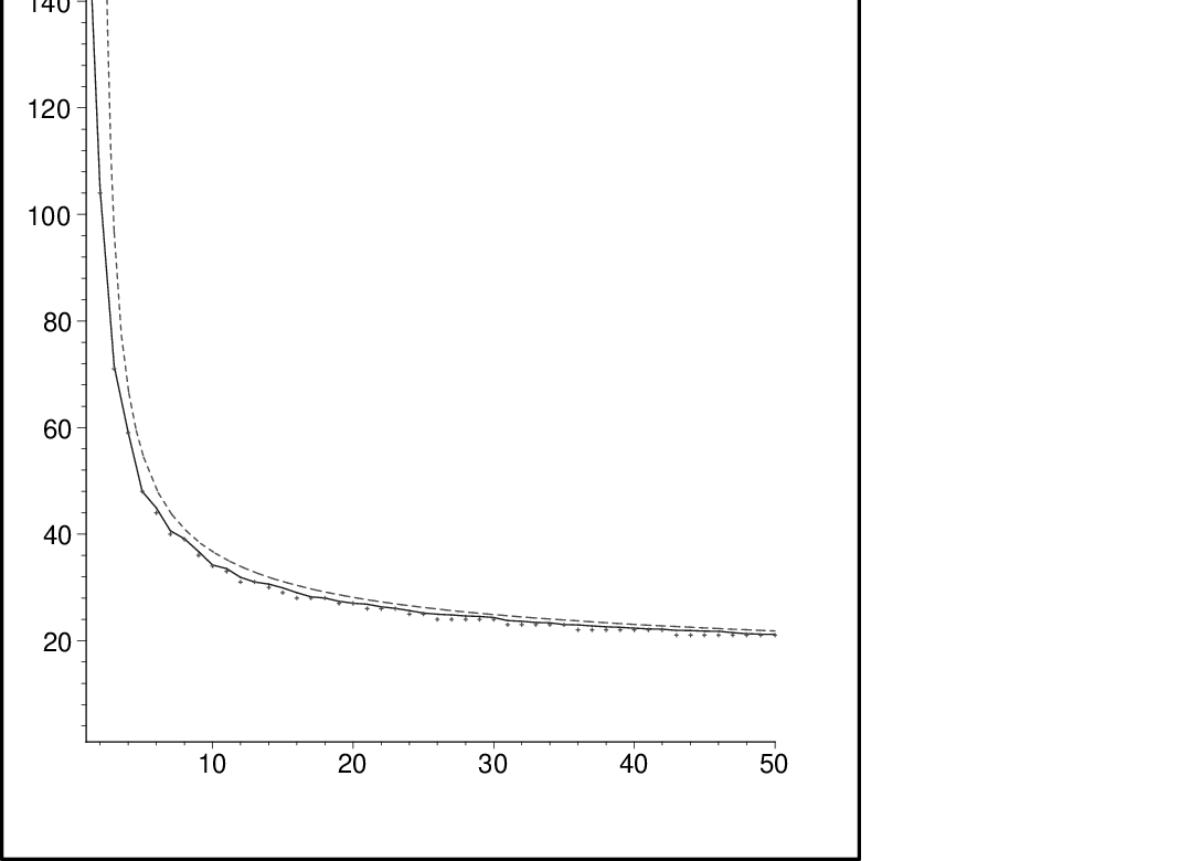
We display below how h2h_{2} varies with nn. Note that h2h_{2} has local maxima when ℓ⁡(n)<ℓ⁡(n+1)\ell(n)<\ell(n+1), i.e. when nn is of the form n=−1+∏k=1jpkn=-1+\prod_{k=1}^{j}p_{k}. Is the h2h_{2} coefficient negative for all nn?

[Uncaptioned image]

One can also ask: what is the sign (and magnitude) of the hkh_{k} coefficient, for very large nn?

6.4. Shellability

Recall that the maximal (with respect to inclusion) faces of a simplicial complex Δ\Delta are called facets, and that a simplicial complex is pure if all its facets have the same dimension (which is then also the dimension of the simplicial complex itself). For a face σ∈Δ\sigma\in\Delta, we let σ¯=2σ\overline{\sigma}=2^{\sigma}, the set of all subsets of σ\sigma, including σ\sigma itself, and the empty set.

Björner and Wachs [2, 3] defines Δ\Delta to be shellable if its facets can be arranged in linear order F1,F2,…,FtF_{1},F_{2},\dots,F_{t} in such a way that the subcomplex ∪i=1k−1Fi¯∩Fk¯\cup_{i=1}^{k-1}\overline{F_{i}}\cap\overline{F_{k}} is pure and of dimension dimFk−1\dim F_{k}-1 for all k=2,…,tk=2,\dots,t. They proved the following [2, Lemma 2.3]:

Lemma 6.8 (Björner-Wachs).

An order F1,F2,…,FtF_{1},F_{2},\dots,F_{t} of the facets of Δ\Delta is a shelling if and only if for every ii and kk with 1≤i≤k1\leq i\leq k there is a jj with 1≤j<k1\leq j<k and an x∈Fkx\in F_{k} such that Fi∩Fk⊆Fj∩Fk=Fk∖{x}.F_{i}\cap F_{k}\subseteq F_{j}\cap F_{k}=F_{k}\setminus{\{x\}}.

We define the lexicographic order on finite subsets of ℙ​ℙ{\mathbb{PP}} in the following way: if

σ=a1,…,ar⊂ℙ​ℙ with ​1≤a1<a2<⋯<ar,\sigma={a_{1},\dots,a_{r}}\subset{\mathbb{PP}}\quad\text{ with }1\leq a_{1}<a_{2}<\dots<a_{r},
τ={b1,…,bs}∈Δ⁡([n]), with ​1≤b1<b2<⋯<bs,\tau={\{b_{1},\dots,b_{s}\}}\in\Delta([n]),\quad\text{ with }1\leq b_{1}<b_{2}<\dots<b_{s},

then σ≥l​e​xτ\sigma\geq_{lex}\tau if either τ=∅\tau=\emptyset or a1>b1a_{1}>b_{1} or σ∖{a1}≥l​e​xτ∖{b1}\sigma\setminus{\{a_{1}\}}\geq_{lex}\tau\setminus{\{b_{1}\}}. Note that ≥l​e​x\geq_{lex} is a Boolean term-order in the sense of Maclagan [13], so

σ≥l​e​xτ⟹σ∪{w}≥l​e​xτ∪{w}≥l​e​xτ.\sigma\geq_{lex}\tau\quad\implies\quad\sigma\cup{\{w\}}\geq_{lex}\tau\cup{\{w\}}\geq_{lex}\tau. (27)
Theorem 6.9.

Δ⁡([n])\Delta([n]) is shellable; the lexicographic order on the facets is a shelling order.

Proof.

Let F1,…,FtF_{1},\dots,F_{t} be the facets in Δ⁡([n]CLOSE\Delta([n] ordered lexicographically. Using the previous lemma, we’ll show that this is a shelling. So pick 1≤i<k≤t1\leq i<k\leq t, and let

Fi∩Fk={a1,…,ar},1≤a1<a2<⋯<ar≤nFi={a1,…,ar}∪{b1,…,bt},1≤b1<ab<⋯<bt≤nFk={a1,…,ar}∪{c1,…,cs},1≤c1<c2<⋯<cs≤n\begin{split}F_{i}\cap F_{k}&={\{a_{1},\dots,a_{r}\}},\quad 1\leq a_{1}<a_{2}<\cdots<a_{r}\leq n\\ F_{i}&={\{a_{1},\dots,a_{r}\}}\cup{\{b_{1},\dots,b_{t}\}},\quad 1\leq b_{1}<a_{b}<\cdots<b_{t}\leq n\\ F_{k}&={\{a_{1},\dots,a_{r}\}}\cup{\{c_{1},\dots,c_{s}\}},\quad 1\leq c_{1}<c_{2}<\cdots<c_{s}\leq n\\ \end{split}

We always have that

r=|Fi∩Fk|<|Fk|=r+s,r={\left\lvert{F_{i}\cap F_{k}}\right\rvert}<{\left\lvert{F_{k}}\right\rvert}=r+s,

since by definition, no facet is contain in another facet. If

|Fk|−|Fi∩Fk|=1,{\left\lvert{F_{k}}\right\rvert}-{\left\lvert{F_{i}\cap F_{k}}\right\rvert}=1,

then we are done, by taking j=ij=i.

So suppose that

|Fk|−|Fi∩Fk|≥2.{\left\lvert{F_{k}}\right\rvert}-{\left\lvert{F_{i}\cap F_{k}}\right\rvert}\geq 2.

This means that s≥2s\geq 2. Since i<ki<k, Fi>l​e​xFkF_{i}>_{lex}F_{k}. We distinguish two cases: some cvc_{v} is a prime power which is not a prime (case 1), or all cvc_{v}’s are prime (case 2).

Case 1: There is some cvc_{v} which is not a prime, thus cv=pδc_{v}=p^{\delta} with δ>1\delta>1, pp a prime. Put

G=(Fk∪{p})∖{cv}.G=\left(F_{k}\cup{\{p\}}\right)\setminus{\{c_{v}\}}.

Then G>l​e​xFkG>_{lex}F_{k}, and since p<cvp<c_{v}, ∏u∈Gu≤n\prod_{u\in G}u\leq n, so G∈Δ⁡([n])G\in\Delta([n]). Clearly,

G∩Fk=Fk∖{cv}.G\cap F_{k}=F_{k}\setminus{\{c_{v}\}}.

Now GG need not be a facet, but it is contained in one, say G⊆FjG\subseteq F_{j}, and by (27) it follows that Fj≥l​e​xFkF_{j}\geq_{lex}F_{k}, whence j<kj<k. Since

Fj∩Fk⊇G∩Fk=Fk∖{cv},F_{j}\cap F_{k}\supseteq G\cap F_{k}=F_{k}\setminus{\{c_{v}\}},

and since, as noted, FkF_{k} can not be contained in another facet, we must have that

Fj∩Fk=Fk∖{cv},F_{j}\cap F_{k}=F_{k}\setminus{\{c_{v}\}},

as desired.

Case 2: Since Fi>l​e​xFkF_{i}>_{lex}F_{k} then b1<c1<c2<⋯<csb_{1}<c_{1}<c_{2}<\dots<c_{s}. If all c1,…,csc_{1},\dots,c_{s} are prime, then gcd⁡(b1,cv)=1\gcd(b_{1},c_{v})=1 for 1≤v≤s1\leq v\leq s. Hence

G=(Fk∪{b1})∖{c1}∈Δ⁡([n]CLOSE.G=\left(F_{k}\cup{\{b_{1}\}}\right)\setminus{\{c_{1}\}}\in\Delta([n].

As before, it sufficies to note that G>l​e​xFkG>_{lex}F_{k} and that G∩Fk=Fk∖{c1}G\cap F_{k}=F_{k}\setminus{\{c_{1}\}} to be able to conclude that there is some j<kj<k such that G⊆FjG\subseteq F_{j},

Fj∩Fk=G∩Fk=Fk∖{c1}.F_{j}\cap F_{k}=G\cap F_{k}=F_{k}\setminus{\{c_{1}\}}.

∎

It follows that all the homology groups of Δ⁡([n])\Delta([n]) are torsion-free.

7. Socle degree, the Gorenstein property, and symmetric Hilbert function for 𝒜[n]\mathcal{A}_{[n]}

7.1. The socle of 𝒜[n]\mathcal{A}_{[n]}

The following easy Lemma was proved in [18].

Lemma 7.1.

Socle⁡(𝒜[n])\mathrm{Socle}(\mathcal{A}_{[n]}) is spanned as a CC-vector space by the set

{ek  1<k≤n,ek⊕f=𝟎 for all f with f(0)≠0}={ek  1<k≤n,kp>n for all p∈ℙ such that gcd(k,p)=1}\left\{\,{e_{k}}\,\vrule\,{1<k\leq n,\,\,e_{k}\oplus f=\mathbf{0}\text{ for all }f\text{ with }f(0)\neq 0}\,\right\}=\\ \left\{\,{e_{k}}\,\vrule\,{1<k\leq n,\,\,kp>n\text{ for all }p\in{\mathbb{P}}\text{ such that }\gcd(k,p)=1}\,\right\} (28)

Furthermore, the eke_{k}’s which span the socle correspond precisely to the facets (maximal faces) σ∈Δ⁡([n])\sigma\in\Delta([n]), σ={pi1a1,…,pirar}\sigma={\{p_{i_{1}}^{a_{1}},\dots,p_{i_{r}}^{a_{r}}\}}, k=pi1a1⋯pirark=p_{i_{1}}^{a_{1}}\cdots p_{i_{r}}^{a_{r}}.

Theorem 7.2.

Let dimℂSocle⁡(𝒜[n])\dim_{\mathbb{C}}\mathrm{Socle}(\mathcal{A}_{[n]}) denote the vector space dimension of the socle of 𝒜[n]\mathcal{A}_{[n]}. Then

limn→∞dimℂSocle⁡(𝒜[n])n=1−12+∑i=1∞1pi−1pi+1∏j=1ipj≈0.60771435951661818\lim_{n\to\infty}\frac{\dim_{\mathbb{C}}\mathrm{Socle}(\mathcal{A}_{[n]})}{n}=1-\frac{1}{2}+\sum_{i=1}^{\infty}\frac{\frac{1}{p_{i}}-\frac{1}{p_{i+1}}}{\prod_{j=1}^{i}p_{j}}\approx 0.60771435951661818 (29)
Proof.

Let ℕ+⁣+={k∈ℕ k>1}{\mathbb{N}}^{++}=\left\{\,{k\in{\mathbb{N}}}\,\vrule\,{k>1}\,\right\}. For all n,k∈ℕ+n,k\in{\mathbb{N}}^{+}, put

In,0=ℕ+⁣+​⋂[n2,n]In,k=ℕ+⁣+​⋂[npk+1,npk)\begin{split}I_{n,0}&={\mathbb{N}}^{++}\bigcap\,\left[\frac{n}{2},n\right]\\ I_{n,k}&={\mathbb{N}}^{++}\bigcap\,\left[\frac{n}{p_{k+1}},\frac{n}{p_{k}}\right)\end{split}

By (28), the integers v∈In,kv\in I_{n,k} correspond to ev∈Socle⁡(𝒜[n])e_{v}\in\mathrm{Socle}(\mathcal{A}_{[n]}) whenever p​v>npv>n for all prime numbers relatively prime to vv. When 2​pk>n2p_{k}>n, In,k=∅I_{n,k}=\emptyset. For the remaining kk’s, we have that In,kI_{n,k} contains approximatively

npk−npk+1\frac{n}{p_{k}}-\frac{n}{p_{k+1}}

integers. Of those integers, only those that are divisible by p1,…,pkp_{1},\dots,p_{k} correspond to ek∈Socle⁡(𝒜[n])e_{k}\in\mathrm{Socle}(\mathcal{A}_{[n]}). Thus, the contribution to the socle from In,kI_{n,k} is approximatively

npi−npi+1∏j=1ipj.\frac{\frac{n}{p_{i}}-\frac{n}{p_{i+1}}}{\prod_{j=1}^{i}p_{j}}.

Clearly, all integers in In,0I_{n,0} are in the socle, which gives a contribution of approximatively n2\frac{n}{2}. Furthermore, for the intervall In,kI_{n,k} to contain any integers, it must have length ≥1\geq 1, i.e. npi−npi+1≥1\frac{n}{p_{i}}-\frac{n}{p_{i+1}}\geq 1. In particular, we must have that npi>1\frac{n}{p_{i}}>1, that is pi<np_{i}<n. Hence, we need only consider π⁡(n)\pi(n) such intervals. For each interval In,kI_{n,k} that does contain integers, the error

−1<(∑x∈In,k∩ℕp1⋯pk|x1)−npk−npk+1p1⋯pk<1.-1<\left(\sum_{\begin{subarray}{c}x\in I_{n,k}\cap{\mathbb{N}}\\ {p_{1}\cdots p_{k}\left\lvert{x}\right.}\end{subarray}}1\right)-\frac{\frac{n}{p_{k}}-\frac{n}{p_{k+1}}}{p_{1}\cdots p_{k}}<1.

Thus, we get that

dimℂSocle⁡(𝒜[n])≈n2+∑k≥1pk≤nnpk−npk+1∏j=1kpj\dim_{\mathbb{C}}\mathrm{Socle}(\mathcal{A}_{[n]})\approx\frac{n}{2}+\sum_{\begin{subarray}{c}k\geq 1\\ p_{k}\leq n\end{subarray}}\frac{\frac{n}{p_{k}}-\frac{n}{p_{k+1}}}{\prod_{j=1}^{k}p_{j}} (30)

with an error <π⁡(n)≈n/log⁡(n)<\pi(n)\approx n/\log(n), from which (29) follows. ∎

In [18] we defined the multiplicative syzygies of 𝒜V\mathcal{A}_{V} as the kernel K2​(V)K_{2}(V) of the ℂ{\mathbb{C}}-linear map

𝒜V+⊗𝒜V+→𝒜V+f⊗g↦f​g\begin{split}\mathcal{A}_{V}^{+}\otimes\mathcal{A}_{V}^{+}&\to\mathcal{A}_{V}^{+}\\ f\otimes g&\mapsto fg\end{split} (31)

We call elements in K2​(V)K_{2}(V) of the form ea⊗ebe_{a}\otimes e_{b} monomial multiplicative syzygies.

Lemma 7.3.

The monomial multiplicative syzygies of 𝒜[n]+\mathcal{A}_{[n]}^{+} correspond to the lattice points

M⁡([n])={(i,j)​ ​ 1<i,j≤n,i​j>n}∪{(i,j)​ ​ 1<i,j≤n,gcd⁡(i,j)>1}M([n])=\left\{\,{(i,j)}\,\vrule\,{1<i,j\leq n,\,ij>n}\,\right\}\cup\left\{\,{(i,j)}\,\vrule\,{1<i,j\leq n,\,\gcd(i,j)>1}\,\right\} (32)

Socle elements correspond to an integer on the xx-axis such that the column supported on it is contained in M⁡([n])M([n]).

Almost all syzygies are monomial, in the sense that

limn→∞|M⁡([n])|dimℂK2​([n])=1\lim_{n\to\infty}\frac{{\left\lvert{M([n])}\right\rvert}}{\dim_{\mathbb{C}}K_{2}([n])}=1 (33)

where K2​([n])K_{2}([n]) is defined as in (31).

Proof.

The first two assertions are obvious. By elementary linear algebra we have that

dimℂK2​([n])=(n−1)2−(n−1).\dim_{\mathbb{C}}K_{2}([n])=(n-1)^{2}-(n-1).

On the other hand,

|M⁡([n])|≥(n−1)2−∫2nn​d​tt≥(n−1)2−n​log⁡n,{\left\lvert{M([n])}\right\rvert}\geq(n-1)^{2}-\int_{2}^{n}\frac{ndt}{t}\geq(n-1)^{2}-n\log n,

so (33) follows. ∎

Below we have plotted the monomial syzygies of 𝒜[30]\mathcal{A}_{[30]}. One can see that 12 is in the socle.

[Uncaptioned image]

7.2. The Gorenstein property for 𝒜[n]\mathcal{A}_{[n]}

A graded Artinian algebra is Gorenstein if and only if the socle is 1-dimensional. A direct computation shows that 𝒜[2]≃ℂ⁡[t]/(t2)\mathcal{A}_{[2]}\simeq{\mathbb{C}}[t]/(t^{2}) is Gorenstein. We note that for n>2n>2, en−1e_{n-1} and ene_{n} must both belong to the socle, which is then at least 2-dimensional, so then 𝒜[n]\mathcal{A}_{[n]} is not Gorenstein.

7.3. Symmetric Hilbert function

A Gorenstein Artinian algebra has a symmetric Hilbert function, hence 𝒜2​(t)=1+t\mathcal{A}_{2}(t)=1+t is symmetric. Can 𝒜[n]​(t)\mathcal{A}_{[n]}(t) be symmetric for other values of nn? If 𝒜[n]​(t)\mathcal{A}_{[n]}(t) symmetric, then cn,ℓ⁡(n)=cn,0=1c_{n,\ell(n)}=c_{n,0}=1, which can only occur when

∏i=1rpi≤n<pr+1​∏i=1r−1pi\prod_{i=1}^{r}p_{i}\leq n<p_{r+1}\prod_{i=1}^{r-1}p_{i} (34)

for some rr: in this case, ℓ⁡(n)=r\ell(n)=r and the only integer in the interval [1,n][1,n] which is the product of rr primes is ∏i=1rpi\prod_{i=1}^{r}p_{i}. Checking these intervals for 1≤r≤101\leq r\leq 10, we get the matches displayed below.

r n 𝒜[n]​(t)\mathcal{A}_{[n]}(t)
1 2 1+t1+t
2 6 1+4​t+t21+4t+t^{2}
2 7 1+5​t+t21+5t+t^{2}
2 8 1+6​t+t21+6t+t^{2}
2 9 1+7​t+t21+7t+t^{2}
3 40 1+19​t+19​t2+t31+19t+19t^{2}+t^{3}

Furthermore, we have [11, §§ 22.11] that the average order and the normal order of ω⁡(n)\omega(n) is log⁡log⁡n\log\log n. For (34) we have that

log⁡log⁡n\displaystyle\log\log n <log⁡log⁡(pr+1​∏i=1r−1pi)\displaystyle<\log\log(p_{r+1}\prod_{i=1}^{r-1}p_{i})
<log⁡r​log⁡(pr+1)\displaystyle<\log r\log(p_{r+1})
=log⁡r+log⁡log⁡pr+1\displaystyle=\log r+\log\log p_{r+1}
<log⁡r+log⁡((r+1)​log⁡2)\displaystyle<\log r+\log((r+1)\log 2)
=log⁡r+log⁡(r+1)+log⁡log⁡2≪r/2\displaystyle=\log r+\log(r+1)+\log\log 2\ll r/2

whenever rr is sufficiently large. If 𝒜[n]​(t)\mathcal{A}_{[n]}(t) were symmetric, it should be centred around r/2r/2. Hence, for sufficiently large rr, 𝒜[n]​(t)\mathcal{A}_{[n]}(t) is not symmetric. There can therefore be only a finite number of nn such that 𝒜[n]​(t)\mathcal{A}_{[n]}(t) is symmetric. We conjecture that the examples tabulated above are in fact all such examples.

8. Basic homological properties

8.1. 𝒜[n]\mathcal{A}_{[n]} as a cyclic ℂ⁡[Y⁡([n])]{\mathbb{C}}[Y([n])]-module

𝒜[n]\mathcal{A}_{[n]} is an Artinian ring and a zero-dimensional module over ℂ⁡[Y⁡([n])]{\mathbb{C}}[Y([n])], with embedding dimension r=π′​(n)r=\pi^{\prime}(n), and homological dimension rr. Recall [11] that r=π′​(n)≈nlog⁡(n)r=\pi^{\prime}(n)\approx\frac{n}{\log(n)}. Furthermore, for the last Betti number we have that

βr​(ℂ⁡[Y⁡([n])],𝒜[n])=dimℂSocle⁡(𝒜[n])≈n2+∑k≥12​pk≤nnpi−npi+1∏j=1ipj≈0.60771435951661818​n,\begin{split}\beta_{r}({\mathbb{C}}[Y([n])],\mathcal{A}_{[n]})&=\dim_{\mathbb{C}}\mathrm{Socle}(\mathcal{A}_{[n]})\\ &\approx\frac{n}{2}+\sum_{\begin{subarray}{c}k\geq 1\\ 2p_{k}\leq n\end{subarray}}\frac{\frac{n}{p_{i}}-\frac{n}{p_{i+1}}}{\prod_{j=1}^{i}p_{j}}\\ &\approx 0.60771435951661818n,\end{split}

by [19, Theorem 12.4] and Theorem 7.2. In fact, the bijection

Torrℂ⁡[Y⁡([n])]​(𝒜[n],ℂ)≃Socle⁡(𝒜[n])\mathrm{Tor}_{r}^{{\mathbb{C}}[Y([n])]}(\mathcal{A}_{[n]},{\mathbb{C}})\simeq\mathrm{Socle}(\mathcal{A}_{[n]})

is degree-preserving, so

βr,j​(ℂ⁡[Y⁡([n])],𝒜[n])=dimℂSocle​(𝒜[n])j.\beta_{r,j}({\mathbb{C}}[Y([n])],\mathcal{A}_{[n]})=\dim_{\mathbb{C}}\mathrm{Socle}(\mathcal{A}_{[n]})_{j}.

For the first betti number we have

β1​(ℂ⁡[Y⁡([n])],𝒜[n])=μ⁡(A[n]+B[n]+C[n])=μ⁡(A[n])+μ⁡(B[n])+μ⁡(C[n]),\beta_{1}({\mathbb{C}}[Y([n])],\mathcal{A}_{[n]})=\mu(A_{[n]}+B_{[n]}+C_{[n]})=\mu(A_{[n]})+\mu(B_{[n]})+\mu(C_{[n]}), (35)

the minimal number of generators of the defining ideal. Clearly

μ⁡(A[n])=r,μ⁡(B[n])=∑i=1r(λi[n]2)\mu(A_{[n]})=r,\qquad\mu(B_{[n]})=\sum_{i=1}^{r}\binom{\lambda_{i}^{[n]}}{2} (36)

8.2. 𝒜[n]\mathcal{A}_{[n]} as a cyclic ℂ⁡[Y⁡([n])¯]{\mathbb{C}}[\overline{Y([n])}]-module

We can also consider 𝒜[n]\mathcal{A}_{[n]} as a zero dimensional module over ℂ⁡[Y⁡([n])¯]{\mathbb{C}}[\overline{Y([n])}], with embedding dimension rr, and infinite homologial dimension. We have that

β1​(ℂ⁡[Y⁡([n])¯],𝒜[n])=μ⁡(B[n]+C[n])=μ⁡(B[n])+μ⁡(C[n]).\beta_{1}({\mathbb{C}}[\overline{Y([n])}],\mathcal{A}_{[n]})=\mu(B_{[n]}+C_{[n]})=\mu(B_{[n]})+\mu(C_{[n]}).
Lemma 8.1.
Pℂ⁡[Y⁡([n])]ℂ⁡[Δ⁡([n])]​(t,𝒖)= the square-free part of ​Pℂ⁡[Y⁡([n])]ℂ⁡[Δ⁡([n])¯]​(t,𝒖)=t−1​∑U⊂V𝒖U​t|U|​𝔓UPℂ⁡[Y⁡([n])¯]𝒜[n]​(t,𝒖)=t−1​∑U⊂V𝒗U​t|U|​𝔓U\begin{split}P^{{\mathbb{C}}[\Delta([n])]}_{{\mathbb{C}}[Y([n])]}(t,{\boldsymbol{u}})&=\text{ the square-free part of }P^{{\mathbb{C}}[\overline{\Delta([n])}]}_{{\mathbb{C}}[Y([n])]}(t,{\boldsymbol{u}})\\ &=t^{-1}\sum_{U\subset V}{\boldsymbol{u}}_{U}t^{{\left\lvert{U}\right\rvert}}\mathfrak{P}_{U}\\ P^{\mathcal{A}_{[n]}}_{{\mathbb{C}}[\overline{Y([n])}]}(t,{\boldsymbol{u}})&=t^{-1}\sum_{U\subset V}{\boldsymbol{v}}_{U}t^{{\left\lvert{U}\right\rvert}}\mathfrak{P}_{U}\end{split} (37)

where

𝔓U=∑i=0|U|t−i​H~i​(Δ​([n])U,ℂ)𝒖U=𝒖U​(u1,…,ur)=∏j∈Uuj,𝒗U=𝒗U​(u1,…,ur)=∏j∈Uuj1−t​uj\begin{split}\mathfrak{P}_{U}&=\sum_{i=0}^{{\left\lvert{U}\right\rvert}}t^{-i}\widetilde{H}^{i}(\Delta([n])_{U},{\mathbb{C}})\\ {\boldsymbol{u}}_{U}&={\boldsymbol{u}}_{U}(u_{1},\dots,u_{r})=\prod_{j\in U}u_{j},\\ {\boldsymbol{v}}_{U}&={\boldsymbol{v}}_{U}(u_{1},\dots,u_{r})=\prod_{j\in U}\frac{u_{j}}{1-tu_{j}}\end{split}
Proof.

It follows from the work of Gasharov, Peeva, and Welker [9] that

βi,𝒂​(ℂ⁡[Y⁡([n])],C⁡[Δ⁡([n])¯])=dimℂH~i−2​(1,𝒚𝒂)L\beta_{i,{\boldsymbol{a}}}({\mathbb{C}}[Y([n])],C[\overline{\Delta([n])}])=\dim_{\mathbb{C}}\widetilde{H}^{i-2}(1,{\boldsymbol{y}}^{{\boldsymbol{a}}})_{L}

where (1,𝒚𝒂)L(1,{\boldsymbol{y}}^{{\boldsymbol{a}}})_{L} is the order complex of the interval (1,𝒚𝒂)(1,{\boldsymbol{y}}^{{\boldsymbol{a}}}) in the sublattice LL of Y∗Y^{*} generated by the minimal generators of A[n]+B[n]+C[n]A_{[n]}+B_{[n]}+C_{[n]}. Similarly,

βi,𝒂​(ℂ⁡[Y⁡([n])],C⁡[Δ⁡([n])])=dimℂH~i−2​(1,𝒚𝒂)L′\beta_{i,{\boldsymbol{a}}}({\mathbb{C}}[Y([n])],C[\Delta([n])])=\dim_{\mathbb{C}}\widetilde{H}^{i-2}(1,{\boldsymbol{y}}^{{\boldsymbol{a}}})_{L^{\prime}}

where (1,𝒚𝒂)L′(1,{\boldsymbol{y}}^{{\boldsymbol{a}}})_{L^{\prime}} is the order complex of the interval (1,𝒚𝒂)(1,{\boldsymbol{y}}^{{\boldsymbol{a}}}) in the sublattice L′L^{\prime} of Y∗Y^{*} generated by the minimal generators of A[n]+B[n]+C[n]A_{[n]}+B_{[n]}+C_{[n]}. Since the square-free monomials form a sublattice SS of Y∗Y^{*}, it follows that L′=L∩SL^{\prime}=L\cap S, hence

βi,𝒂​(ℂ⁡[Y⁡([n])],C⁡[Δ⁡([n])])={0𝒂​ not square-freeβi,𝒂​(ℂ⁡[Y⁡([n])],ℂ⁡[Δ⁡([n])¯])𝒂​ square-free\beta_{i,{\boldsymbol{a}}}({\mathbb{C}}[Y([n])],C[\Delta([n])])=\begin{cases}0&{\boldsymbol{a}}\text{ not square-free}\\ \beta_{i,{\boldsymbol{a}}}({\mathbb{C}}[Y([n])],{\mathbb{C}}[\overline{\Delta([n])}])&{\boldsymbol{a}}\text{ square-free}\end{cases}

The remaining results are immediate from the formulaes in the appendix. ∎

Theorem 8.2.

The Castelnuovo-Mumford regularity of the ℂ⁡[Y⁡([n])¯]{{\mathbb{C}}[\overline{Y([n])}]}-module 𝒜[n]{\mathcal{A}_{[n]}} (or, equivalently, the Castelnuovo-Mumford regularity of the ℂ⁡[Y⁡([n])]{{\mathbb{C}}[Y([n])]}-module ℂ⁡[Δ⁡([n])]{{\mathbb{C}}[\Delta([n])]}) is 1+v⁡(n)1+v(n), where v⁡(n)v(n) is as defined in (14).

Proof.

It follows from (37) and (14) that the Castelnuovo-Mumford regularity is equal to

1+max⁡{i​ ​∃U:H~i​(Δ​([n])U,ℂ)≠0}=1+v⁡(n).1+\max\left\{\,{i}\,\vrule\,{\exists U:\widetilde{H}^{i}(\Delta([n])_{U},{\mathbb{C}})\neq 0}\,\right\}=1+v(n).

∎

8.3. The Stanley-Reisner ring ℂ⁡[Δ⁡([n])]{{\mathbb{C}}[\Delta([n])]}

The Stanley-Reisner ℂ⁡[Δ⁡([n])]{{\mathbb{C}}[\Delta([n])]} is a ring of dimension dimΔ⁡([n])+1=ℓ⁡(n)\dim\Delta([n])+1=\ell(n) and a ℂ⁡[Y⁡([n])]{{\mathbb{C}}[Y([n])]}-module of homological dimension r−1r-1. From the formulaes in the appendix we get that

μ⁡(B[n])+μ⁡(C[n])=β1​(ℂ⁡[Y⁡([n])¯],𝒜[n])=β1​(ℂ⁡[Y⁡([n])],ℂ⁡[Δ⁡([n])])=∑U⊂VdimℂH~|U|−2​(Δ​([n])U,ℂ)=∑i=0r−2∑|U|=i+2dimℂH~i​(Δ​([n])U,ℂ)\begin{split}\mu(B_{[n]})+\mu(C_{[n]})&=\beta_{1}({\mathbb{C}}[\overline{Y([n])}],{\mathcal{A}_{[n]}})\\ &=\beta_{1}({{\mathbb{C}}[Y([n])]},{\mathbb{C}}[\Delta([n])])\\ &=\sum_{U\subset V}\dim_{\mathbb{C}}\widetilde{H}^{{\left\lvert{U}\right\rvert}-2}(\Delta([n])_{U},{\mathbb{C}})\\ &=\sum_{i=0}^{r-2}\sum_{{\left\lvert{U}\right\rvert}=i+2}\dim_{\mathbb{C}}\widetilde{H}^{i}(\Delta([n])_{U},{\mathbb{C}})\end{split} (38)

8.4. The Koszul property

Since A[n]A_{[n]} and B[n]B_{[n]} are quadratic, and we know for which ii the reduced simplicial homology H~i​(Δ​([n])U,ℂ)\widetilde{H}^{i}(\Delta([n])_{U},{\mathbb{C}}) can be non-zero, we get

Corollary 8.3.

The maximal degree of a minimal generator of C[n]C_{[n]}, for n>2n>2, is max⁡{2,v⁡(n)}\max{\{2,\,v(n)\}}. In particular, C[n]C_{[n]} is quadratic for n<15n<15. Furthermore,

μ⁡(C[n])=∑i=0r−2∑|U|=i+2dimℂH~i​(Δ​([n])U,ℂ)−∑i=1r(λi[n]2)\mu(C_{[n]})=\sum_{i=0}^{r-2}\sum_{{\left\lvert{U}\right\rvert}=i+2}\dim_{\mathbb{C}}\widetilde{H}^{i}(\Delta([n])_{U},{\mathbb{C}})-\sum_{i=1}^{r}\binom{\lambda_{i}^{[n]}}{2} (39)
Proposition 8.4.

𝒜[n]\mathcal{A}_{[n]} is Koszul if and only if n<15n<15.

Proof.

𝒜[n]\mathcal{A}_{[n]} is a monomial algebra, and is quadratic iff n<15n<15. Thus by a result of Fröberg [7], 𝒜[n]\mathcal{A}_{[n]} is Koszul iff n<15n<15. ∎

Appendix A Homological formulaes for Stanley-Reisner rings and indicator algebras

In this appendix, we assume that Δ\Delta is a simplicial complex on the finite set W={1,…,r}W={\{1,\dots,r\}}. For U⊂WU\subset W, ΔU={σ∈Δ σ⊂U}\Delta_{U}=\left\{\,{\sigma\in\Delta}\,\vrule\,{\sigma\subset U}\,\right\}; it is a simplicial complex on UU. We denote by H~i​(ΔU,ℂ)\widetilde{H}^{i}(\Delta_{U};\,{\mathbb{C}}) the reduced simplicial homology. Note that when ∅∈Δ\emptyset\in\Delta, H~−1​(Δ∅,ℂ)≃ℂ\widetilde{H}^{-1}(\Delta_{\emptyset};\,{\mathbb{C}})\simeq{\mathbb{C}}.

We write S=ℂ⁡[x1,…,xr]S={\mathbb{C}}[x_{1},\dots,x_{r}], S¯=ℂ⁡[x1,…,xr](x12,…,xr2)\bar{S}=\frac{{\mathbb{C}}[x_{1},\dots,x_{r}]}{(x_{1}^{2},\dots,x_{r}^{2})}, and EE for the exterior algebra on the vector space of linear forms in SS. Then ℂ⁡[Δ]{\mathbb{C}}[\Delta] is a cyclic SS-module, ℂ⁡[Δ¯]{\mathbb{C}}[\overline{\Delta}] a cyclic S¯\bar{S}-module, and ℂ​{Δ}{\mathbb{C}}\{\Delta\} a cyclic EE-module. CC is a module over all these rings.

Theorem A.1 (Hochster, [12]).

Let βi\beta_{i} denote the ii’th Betti number of ℂ⁡[Δ]{\mathbb{C}}[\Delta] (in a minimal free resolution of ℂ⁡[Δ]{\mathbb{C}}[\Delta] as an SS-module), and let βi,𝛂\beta_{i,{\boldsymbol{\alpha}}} denote the corresponding multi-graded Betti number. Then

βi,𝜶={0 if ​𝜶​ is not square-free,dimℂH~|U|−i−1​(ΔU,ℂ) if ​𝜶​ is square-free with ​supp​(𝜶)=Uβi=∑U⊂WdimℂH~|U|−i−1​(ΔU,ℂ)\begin{split}\beta_{i,{\boldsymbol{\alpha}}}&=\begin{cases}0&\text{ if }{\boldsymbol{\alpha}}\text{ is not square-free},\\ \dim_{\mathbb{C}}\widetilde{H}^{{\left\lvert{U}\right\rvert}-i-1}(\Delta_{U};\,{\mathbb{C}})&\text{ if }{\boldsymbol{\alpha}}\text{ is square-free with }\mathrm{supp}({\boldsymbol{\alpha}})=U\end{cases}\\ \beta_{i}&=\sum_{U\subset W}\dim_{\mathbb{C}}\widetilde{H}^{{\left\lvert{U}\right\rvert}-i-1}(\Delta_{U};\,{\mathbb{C}})\\ \end{split} (40)

Thus the Poincaré-Betti series is

PSℂ⁡[Δ]​(t,𝒖)=∑U⊂W∏j∈Uuj​∑i=−∞∞ti​dimℂ(H~|U|−i−1​(ΔU,ℂ))P^{{\mathbb{C}}[\Delta]}_{S}(t,{\boldsymbol{u}})=\sum_{U\subset W}\prod_{j\in U}u_{j}\sum_{i=-\infty}^{\infty}t^{i}\dim_{\mathbb{C}}\left(\widetilde{H}^{{\left\lvert{U}\right\rvert}-i-1}(\Delta_{U};\,{\mathbb{C}})\right) (41)

Note that H~j​(ΔU,ℂ)=0\widetilde{H}^{j}(\Delta_{U};\,{\mathbb{C}})=0 for j<−1j<-1, j≥n−1j\geq n-1, so the above sum is finite.

Theorem A.2 (Aramova-Herzog-Hibi [1]).

Let βi\beta_{i} denote the ii’th Betti number of ℂ​{Δ}{\mathbb{C}}\{\Delta\} (in a minimal free resolution of ℂ​{Δ}{\mathbb{C}}\{\Delta\} as an EE-module), and let βi,𝛂\beta_{i,{\boldsymbol{\alpha}}} denote the corresponding multi-graded Betti number. Then

βi,𝜶=dimℂH~|𝜶|−i−1​(ΔU,ℂ), where ​U=supp⁡(𝜶)\beta_{i,{\boldsymbol{\alpha}}}=\dim_{\mathbb{C}}\widetilde{H}^{{\left\lvert{{\boldsymbol{\alpha}}}\right\rvert}-i-1}(\Delta_{U};\,{\mathbb{C}}),\quad\text{ where }U=\mathrm{supp}({\boldsymbol{\alpha}}) (42)
Corollary A.3.

In the above situation,

βi=∑U⊂W∑ℓ=−1|U|−1(ℓ+iℓ+1+i−|U|)​dimℂH~|U|−i−1​(ΔU,ℂ)\beta_{i}=\sum_{U\subset W}\sum_{\ell=-1}^{{\left\lvert{U}\right\rvert}-1}\binom{\ell+i}{\ell+1+i-{\left\lvert{U}\right\rvert}}\dim_{\mathbb{C}}\widetilde{H}^{{\left\lvert{U}\right\rvert}-i-1}(\Delta_{U};\,{\mathbb{C}}) (43)
Lemma A.4 (Sköldberg [15]).
PEℂ​{Δ}​(t,u1,…,ur)=PSℂ⁡[Δ]​(t,ui1−t​u1,…,ur1−t​ur)P^{{\mathbb{C}}\{\Delta\}}_{E}(t,u_{1},\dots,u_{r})=P^{{\mathbb{C}}[\Delta]}_{S}(t,\frac{u_{i}}{1-tu_{1}},\dots,\frac{u_{r}}{1-tu_{r}}) (44)
Corollary A.5.
PEℂ​{Δ}​(t,𝒖)=∑U⊂W∏j∈Uuj1−t​uj​∑i=−∞∞ti​dimℂ(H~|U|−i−1​(ΔU,ℂ))P^{{\mathbb{C}}\{\Delta\}}_{E}(t,{\boldsymbol{u}})=\sum_{U\subset W}\prod_{j\in U}\frac{u_{j}}{1-tu_{j}}\sum_{i=-\infty}^{\infty}t^{i}\dim_{\mathbb{C}}\left(\widetilde{H}^{{\left\lvert{U}\right\rvert}-i-1}(\Delta_{U};\,{\mathbb{C}})\right) (45)
Definition A.6.

For U⊂WU\subset W, we introduce the notation

𝒖U=𝒖U​(u1,…,ur)=∏j∈Uuj,𝒗U=𝒗U​(u1,…,ur)=∏j∈Uuj1−t​uj,𝔓U=∑i=−1∞t−i​H~i​(ΔU,ℂ)\begin{split}{\boldsymbol{u}}_{U}&={\boldsymbol{u}}_{U}(u_{1},\dots,u_{r})=\prod_{j\in U}u_{j},\\ {\boldsymbol{v}}_{U}&={\boldsymbol{v}}_{U}(u_{1},\dots,u_{r})=\prod_{j\in U}\frac{u_{j}}{1-tu_{j}},\\ \mathfrak{P}_{U}&=\sum_{i=-1}^{\infty}t^{-i}\widetilde{H}^{i}(\Delta_{U},{\mathbb{C}})\end{split} (46)
Corollary A.7.
PSℂ⁡[Δ]​(t,𝒖)=t−1​∑U⊂W𝒖U​t|U|​𝔓UPEℂ​{Δ}​(t,𝒖)=t−1​∑U⊂W𝒗U​t|U|​𝔓U\begin{split}P^{{\mathbb{C}}[\Delta]}_{S}(t,{\boldsymbol{u}})&=t^{-1}\sum_{U\subset W}{\boldsymbol{u}}_{U}t^{{\left\lvert{U}\right\rvert}}\mathfrak{P}_{U}\\ P^{{\mathbb{C}}\{\Delta\}}_{E}(t,{\boldsymbol{u}})&=t^{-1}\sum_{U\subset W}{\boldsymbol{v}}_{U}t^{{\left\lvert{U}\right\rvert}}\mathfrak{P}_{U}\\ \end{split} (47)
Lemma A.8 (Sköldberg, [15]).
PS¯ℂ⁡[Δ¯]​(t,𝒖)=PEℂ​{Δ}​(t,𝒖)Pℂ⁡[Δ¯]ℂ​(t,𝒖)=Pℂ​{Δ}ℂ​(t,𝒖)\begin{split}P^{{\mathbb{C}}[\overline{\Delta}]}_{\bar{S}}(t,{\boldsymbol{u}})&=P^{{\mathbb{C}}\{\Delta\}}_{E}(t,{\boldsymbol{u}})\\ P^{{\mathbb{C}}}_{{\mathbb{C}}[\overline{\Delta}]}(t,{\boldsymbol{u}})&=P^{{\mathbb{C}}}_{{\mathbb{C}}\{\Delta\}}(t,{\boldsymbol{u}})\end{split} (48)

References

  • [1] Annetta Aramova, Jürgen Herzog, and Takayuki Hibi. Gotzman theorems for exterior algebras and combinatorics. Journal of Algebra, 191:174–211, 1997.
  • [2] Anders Björner and Michelle L. Wachs. Shellable nonpure complexes and posets. I. Trans. Amer. Math. Soc., 348(4):1299–1327, 1996.
  • [3] Anders Björner and Michelle L. Wachs. Shellable nonpure complexes and posets. II. Trans. Amer. Math. Soc., 349(10):3945–3975, 1997.
  • [4] E. D. Cashwell and C. J. Everett. The ring of number-theorethic functions. Pacific Journal of Mathematics, 9:975–985, 1959.
  • [5] Jean-Guillaume Dumas, Frank Heckenbach, B. David Saunders, and Volkmar Welker. Simplicial Homology. GAP package (http://www.cis.udel.edu/~dumas/Homology/).
  • [6] S. Eliahou and M. Kervaire. Minimal resolutions of some monomial ideals. Journal of Algebra, 129:1–25, 1990.
  • [7] Ralf Fröberg. Determination of a class of Poincaré series. Math. Scand., 37(1):29–39, 1975.
  • [8] The GAP Group. GAP – Groups, Algorithms, and Programming, Version 4.3, 2002. (http://www.gap-system.org).
  • [9] Vesselin Gasharov, Irena Peeva, and Volkmar Welker. The lcm-lattice in monomial resolutions. Math. Res. Lett., 6(5-6):521–532, 1999.
  • [10] Daniel R. Grayson and Michael E. Stillman. Macaulay 2. Computer algebra program, available at http://www.math.uiuc.edu/Macaulay2/.
  • [11] G. H. Hardy and E. M. Wright. An introduction to the theory of numbers. The Clarendon Press Oxford University Press, New York, fifth edition, 1979.
  • [12] Melvin Hochster. Cohen-Macaulay rings, combinatorics, and simplicial complexes. In Ring theory, II (Proc. Second Conf., Univ. Oklahoma, Norman, Okla., 1975), pages 171–223. Lecture Notes in Pure and Appl. Math., Vol. 26. Dekker, New York, 1977.
  • [13] Diane Maclagan. Boolean term orders and the root system Bn{B}_{n}. Order, 15(3):279–295, 1998/99.
  • [14] W. Narkiewicz. On a class of arithmetical convolutions. Colloq. Math., 10:81–94, 1963.
  • [15] Emil Sköldberg. Monomial Golod Quotients of Exterior Algebras. Journal of Algebra, 218:183–189, 1998.
  • [16] Jan Snellman. Truncations of the ring of number-theorethic functions. Homology, Homotopy and Applications, 2:17–27, 2000, math.NT/9904143.
  • [17] Jan Snellman. The ring of arithmetical functions with unitary convolution: Divisorial and topological properties. Research Reports in Mathematics 4/2002, Department of Mathematics, Stockholm University, apr 2002, math.RA/0201082.
  • [18] Jan Snellman. The ring of arithmetical functions with unitary convolution: General truncations. Research Reports in Mathematics 6/2002, Department of Mathematics, Stockholm University, may 2002, math.RA/0205242.
  • [19] Richard P. Stanley. Combinatorics and Commutative Algebra, volume 41 of Progress in Mathematics. Birkhäuser, 2 edition, 1996.
  • [20] Gérald Tenenbaum. Introduction to analytic and probabilistic number theory. Cambridge Univeristy Press, 1995.