Combinatorial properties of Thompson’s group Thanks: The first author acknowledges support from PSC-CUNY grant #63438-0032. The second author would like to thank the University of Utah for their hospitality during the writing of this paper.
Abstract.
We study some combinatorial properties of the word metric of Thompson’s group in the standard two generator finite presentation. We explore connections between the tree pair diagram representing an element of , its normal form in the infinite presentation, its word length, and minimal length representatives of it. We estimate word length in terms of the number and type of carets in the tree pair diagram and show sharpness of those estimates. In addition we explore some properties of the Cayley graph of with respect to the two generator finite presentation. Namely, we exhibit the form of “dead end” elements in this Cayley graph, and show that it has no “deep pockets”. Finally, we discuss a simple method for constructing minimal length representatives for strictly positive or negative words.
1. Introduction
Thompson’s group has been studied extensively in many different branches of mathematics, including group theory, dynamics, homotopy theory and logic. Algebraically, it is most commonly understood in two different forms: via a finite presentation and an infinite presentation. The infinite presentation has simple relators which are conveniently manipulated and understood, as well as a unique normal form for elements. The finite presentation has two generators and two relators, but the relators are more complicated and there is no longer a convenient set of normal forms. The elements of can also be interpreted as pairs of finite binary rooted trees with the same number of carets.
In this paper we discuss many interesting combinatorial properties of Thompson’s group . These properties are derived from the relationship between the normal form of elements of and the pairs of finite binary rooted trees used to represent elements of . The combinatorial properties we describe have applications to estimating word length in , counting and determining caret types and lead to algorithms for constructing minimal length paths. The sections of this paper are organized as follows.
- •
In Section 2 we present brief introduction to Thompson’s group , including Fordham’s method of calculating word length [6]. We detail the bijective process which transforms a tree pair diagram representing an element of into its unique normal form.
- •
In Section 3 we apply Fordham’s method to immediately obtain an estimate of the word length of an element from the tree pair diagram representing in the word metric arising from the finite presentation . We give examples which show that the constants in the estimate are sharp.
- •
In Section 4 we use Fordham’s method of calculating word length to explore an interesting phenomenon which occurs in the Cayley graph of with respect to the standard two generator finite presentation. Namely, there are dead end elements with the property that for all generators , where denotes word length. Fordham [6] remarks that some of these dead end elements have a particular form; we give a general form for all dead end elements in and describe some limits to stronger forms of this behavior, called “deep pockets.”
- •
In Section 5 describe the combinatorial relationship between the normal form of an element and the number and types of carets in the tree pair diagram representing .
- •
In Section 6 we present a method of constructing minimal length paths in the standard two generator presentation for strictly positive or negative words in .
2. Thompson’s group
Thompson’s group is best understood combinatorially using the two presentations mentioned above, the finite presentation
and the infinite presentation
A convenient set of normal forms for elements of in the infinite presentation is given by where , and . To obtain a unique normal form for each element, we add the condition that when both and occur, so does or , as discussed by Brown and Geoghegan [1]. We will always mean unique normal form when we refer to a word in normal form.
Analytically, we can regard as the group of orientation-preserving piecewise-linear homeomorphisms from to itself where each homeomorphism has only finitely many singularities of slope, all such singularities lie in the dyadic rationals , and, away from the singularities, the slopes are powers of .
2.1. Tree pair diagrams
An element of can be interpreted geometrically via a tree pair diagram, which is a pair of rooted binary trees , each with the same number of exposed leaves, as described in Cannon, Floyd and Parry [4]. An exposed leaf ends in a vertex of valence , and we number these exposed leaves from left to right, beginning with . We refer to a node together with the two downward-directed edges from the node as a caret. A caret may have a right child, a caret which is attached to the right edge of . We can similarly define the left child of the caret . The set of all carets which stem from the right leaf of a caret is called the right subtree of , and we can analogously define the left subtree of .

In a tree pair , the tree is called the negative tree and the positive tree. This terminology is explained further in §2.2 below. The equivalence between tree pair diagrams and homeomorphisms of is described in [4]. In figure 1 we give the tree pair diagrams for the generators and of . In §2.2 below the correspondence between the trees and the elements is explained.
A tree pair diagram is unreduced if both and contain a caret with two exposed leaves numbered and . There are many tree pair diagrams representing the same element of but each element has a unique reduced tree pair diagram representing it. When we write to represent an element of , we are assuming that the tree pair is reduced.
2.2. Exponents in tree pair diagrams
There is a bijective correspondence between the tree pair diagram of and the normal form of , described in [4]. In the tree pair , number the exposed leaves of and from left to right, beginning with . The exponent of the leaf labelled , written , is defined as the length of the maximal path consisting entirely of left edges from which does not reach the right side of the tree. Note that for an exposed leaf labelled which is a right leaf of a caret, as there is no path consisting entirely of left edges originating from . In figure 1, number the exposed leaves of the trees in the pair representing from left to right, beginning with . Then the exponents of the leaves of are all , and the exponents of the leaves of are , in order. We refer the reader to [5] for a more detailed example of computing exponents in a tree.
Once the exponents of the leaves in and have been computed, the normal form of the element is easily obtained. The positive part of the normal form of is
where is the number of exposed leaves in either tree, and the exponents are obtained from the leaves of . The negative part of the normal form of is similarly found to be
where the exponents are now computed from the leaves of . Note that many of the exponents in the normal form as given above may be zero.
Similarly, given an element in normal form with respect to the infinite generating set, it is possible to construct a tree pair diagram () so that each leaf has the correct exponent. If is a right caret with a single exposed left leaf labelled , then by definition. Thus, arbitrarily many right carets with no left subtrees can be added to either or without affecting the normal form to ensure that both trees have the same number of carets, and thus equivalently the same number of exposed leaves.
2.3. Fordham’s method of calculating word length
For an element of , we let denote the word length of with respect to the word metric arising from the finite presentation . Fordham [6] presents a method of calculating based on the trees and in the tree pair diagram representing . He defines seven types of carets that can be found in a rooted binary tree, and an intricate system of weights assigned to different pairs of caret types, which sum to . A detailed example of calculating in this way can be found in [5].
Let be a finite rooted binary tree. The left side of is the maximal path of left edges beginning at the root of . Similarly, we have the right side of . A caret in is a left caret if its left edge is on the left side of the tree, a right caret if it is not the root and its right edge is on the right side of the tree, and an interior caret otherwise. The carets and the exposed leaves of are numbered independently, according to different methods. As above, the exposed leaves are numbered from left to right, beginning with . The carets in are numbered according to the infix ordering of nodes. Caret is a left caret with an exposed left leaf numbered in the leaf numbering. According to the infix scheme, we number the left children of a caret before the caret itself, and number the right children after numbering the caret.

In figure 2 we give an example of a tree whose carets are numbered according to the infix numbering method. More examples of trees whose carets are numbered in this way can be found in [5].
Fordham classifies carets into seven disjoint types, as follows:
- (1)
. The first caret on the left side of the tree, with caret number . Every tree has exactly one caret of type .
- (2)
. Any left caret other than the one numbered .
- (3)
. An interior caret which has no right child.
- (4)
. An interior caret which has a right child.
- (5)
. Any right caret numbered with the property that caret is an interior caret.
- (6)
. A right caret which is not an but for which there is a higher numbered interior caret.
- (7)
. A right caret with no higher-numbered interior carets.
The root caret is always considered to be a left caret and will be of type unless it has no left children, in which case it would be the single caret of type .
The main result of Fordham [6] is that the word length of can be computed from knowing the caret types of the carets in the two trees, as long as they form a reduced pair, via the following process. We number the carets according to the infix method described above, and for each with we form the pair of caret types consisting of the type of caret number in and the type of caret number in . The single caret of type in will be paired with the single caret of type in , and for that pairing we assign a weight of 0. For all other caret pairings, we assign weights according to the following table.
| 0 | 2 | 2 | 1 | 1 | 3 | |
| 2 | 2 | 2 | 1 | 1 | 3 | |
| 2 | 2 | 2 | 1 | 3 | 3 | |
| 1 | 1 | 1 | 2 | 2 | 2 | |
| 1 | 1 | 3 | 2 | 2 | 4 | |
| 3 | 3 | 3 | 2 | 4 | 4 |
The main result of Fordham [6] is the following theorem.
Theorem 2.1 (Fordham [6] 2.5.1).
Given a word described by the reduced tree pair diagram , the length of the word with respect to the generating set is the sum of the weights of the caret pairings in .
2.4. How generators affect a tree pair diagram
The strength of Fordham’s method is that it requires only geometric information about the pair of trees representing an element to determine . Beginning with an element , if we knew the reduced pair of trees which represented for , we could deduce the word length of . We now discuss how the tree pair diagrams for and are related.
We begin with a lemma from Fordham [6] which states under fairly broad conditions, that when applying a generator to a tree pair exactly one pair of caret types will change.
Lemma 2.2 (Fordham [6], Lemma 2.3.1).
Let be a reduced pair of trees, each having carets, representing an element , and any generator of .
- (1)
If , we require that the left subtree of the root of is nonempty.
- (2)
If , we require that the right subtree of the root of is nonempty.
- (3)
If , we require that the left subtree of the right child of the root of is nonempty.
- (4)
If , we require that the right subtree of the right child of the root of is nonempty.
If the reduced tree pair diagram for also has carets, then there is exactly one with so that the pair of caret types of caret changes when is applied to .
We now begin to understand geometrically the action of a generator of on a reduced tree pair , and the corresponding change in normal form. In this section we will assume that the conditions of lemma 2.2 are met by the generic elements with which we begin. The following geometric lemma describing the action of the generators in on an element is proven in [5]. Let denote the caret which is the right child of the root caret of , and the left child of the root.


Lemma 2.3 ([5], Lemmas 2.6,2.7).
Notice that in all of the descriptions above, the tree from the pair is not affected when a generator is applied to . This is not true in general for reduced tree pair diagrams not satisfying the conditions of lemma 2.2. In general, can be affected in exactly three ways:
- (1)
when has a single left edge, and the generator is ,
- (2)
when the left subtree of the right child of the root caret of is empty, and the generator is , or
- (3)
if the generator is and the pair of trees corresponding to is not reduced.
When the generators and are applied to an element , the change in normal form is straightforward. Namely, remains in normal form. If in normal form, then in normal form. Otherwise, in normal form, where . In this case, , where is the shift map which increases the index of each generator in the normal form of .
We now determine the change in normal form when a generator is applied to an element in normal form. The following lemmas are proven in [5].
Lemma 2.4 (The normal form of , [5], Lemma 2.4).
Let be represented by the tree pair , and have normal form . Then has normal form
| (1) |
where we might have . If the root caret of has right and left subtrees and respectively, then is smallest leaf number in .
2.5. Calculating distance between elements using tree pair diagrams
When viewing elements of as homeomorphisms of it is clear that inversion and group multiplication correspond to inversion and composition of homeomorphisms. We now interpret inversion and group multiplication in terms of tree pair diagrams.
Inversion of a group element given by a tree pair diagram is simply the tree pair diagram . This can be seen easily from the normal form and is interpreted via homeomorphisms in [4].
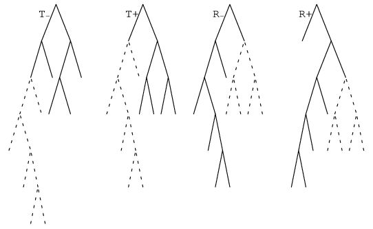
Given two group elements with tree pair diagrams and we would like to form their product by a process consistent with composition of homeomorphisms. When and are identical, we see that is represented by the (possibly unreduced) tree pair diagram . This corresponds to composition of the piecewise linear homeomorphisms represented by and , where .
When and differ, we create temporary, unreduced representatives of and in which the new trees and are identical. Then the composition is carried out in the same manner as described above.
Figure 5 gives an example of the composition of two elements of . The solid lines indicate the original carets and the dashed lines indicate carets added to perform the composition which create unreduced representatives of both elements. To measure the distance between two elements of , we use the word metric on the product to obtain the metric .
3. Estimating the word metric
It follows immediately from the chart in §2.3 that the word length of can be estimated in terms of the number of carets in either tree. This estimate is analogous to the one given by Burillo, Cleary and Stein [2] which has multiplicative constant for the upper bound.
Theorem 3.1.
Let be represented by a tree pair in which each tree has carets. Then
Proof.
We first note that every reduced tree pair has a caret type pair of weight . Also, it is possible to have the last caret type pair be which also has weight . (The only instance in which this does not happen is when the root caret of or has no right subtree.) For the upper bound, we can ignore the first caret pair, and looking at the chart in §2.3, we see that the maximum weight of any other pair of caret types is . Thus the word length of is at most .
To compute the lower bound, we ignore pairs of carets of type and . Any other pair of caret types has weight at least , and the lower bound is easily obtained. ∎
It is natural to ask if the multiplicative coefficient of 4 in theorem 3.1 can be improved to , since looking at the chart in §2.3 we see that there are very few entries which are ; that is, very few caret type pairs actually have weight . The answer is no; one can produce words which get extremely close to the bound of by pairing and carets in a particular way.

Example 3.2.
Words of the form where is a positive integer realize the upper bound of in theorem 3.1.
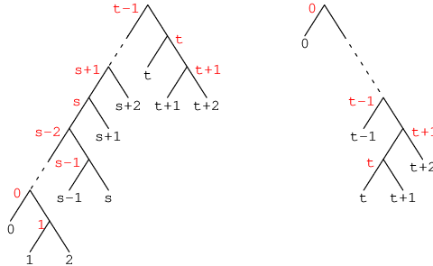
Words of the above form are represented by the tree pair diagram given in figure 6. They are constructed so that most carets in are of type and are paired with carets of type in , to give a weight of per pair for most caret pairs. The weights of the different caret pairs are summarized in the following table.
| Caret numbers | Caret types | Weight per caret | Total weight |
|---|---|---|---|
| 0 | 0 | 0 | |
| 4 | |||
| m | 2 | 2 | |
| m+1 | 0 | 0 |
The total weight of a word of this form is . The total number of carets is , so these examples, which have weight , show that for large the multiplicative coefficient of 4 in Theorem 3.1 is optimal.
It is also natural to wonder if the lower bound can be realized; that is, are there examples of words where the number of carets is exactly two more than the word length ? This will always be true for words of the form (but not for ). In the following example, we show that it can also be true for more complicated words.
Example 3.3.
Words of the form where , is odd, and is chosen so that the root caret of is caret number realize the lower bound of theorem 3.1.
These words are represented by tree pairs of the form given in Figure 7. The weights of the caret type pairs are summarized in the following table.
| Caret numbers | Caret types | Weight per caret |
|---|---|---|
| 0 | 0 | |
| , even numbers | 1 | |
| , odd numbers | 1 | |
| 1 | ||
| 1 | ||
| 1 | ||
| 0 |
It is clear from the table that the total weight of the word is two less than the number of carets, realizing the lower bound of theorem 3.1.
Theorem 3.1 has an immediate improvement for strictly positive or negative words.
Corollary 3.4.
Let be a strictly positive or negative word, represented by a tree having carets. Then
Proof.
Since is strictly positive or negative, one of the trees in the tree pair diagram for consists entirely of carets (excepting the root caret which is of type and does not contribute to the total weight of the word.) Thus, we only need to look at the first column of the chart in §2.3 to assign weights to the different carets. We notice that the maximum weight in the first column of this chart is , and the corollary follows. ∎
4. Dead end elements
We now consider the Cayley graph of with respect to the finite generating set . Fordham describes a family of elements which we call dead end elements that have the property that all four generators and decrease the word length of . They are “dead ends” in the sense that a geodesic ray in from the identity cannot be pass through them, that is, a ray through a dead end element can no longer be geodesic past . We prove that all dead end elements have a particular form, which is slightly more general than the examples given by Fordham [6], and discuss other possible dead end behavior in .
4.1. The form of dead end elements in
Theorem 4.1.
All dead end elements in are given by tree pairs of the form in Figure 8 where the subtrees and are nonempty.

The key step in the proof of theorem 4.1 is enumerating the conditions under which a specific generator decreases the word length of an element. This requires a detailed understanding of caret pairings as well as how a generator can affect a tree pair. We begin with a lemma of Fordham [6] which states that if does not satisfy the appropriate condition of lemma 2.2, then . This allows us to consider only words satisfying all the conditions of lemma 2.2 as possible dead end words.
Lemma 4.2 (Fordham [6], Lemma 2.4.2).
Let be a generator of , and a word not satisfying the condition in lemma 2.2 corresponding to . Then .
Thus, if does not satisfy all the conditions of lemma 2.2, then is not a candidate for a dead end word.
We let and denote the left and right carets, respectively, of the root caret of . Similarly, let and denote the right and left children, respectively, of the caret . Let and denote the left and right subtrees, respectively, of the root caret of . Continue this notation to let denote the left subtree of , etc. In general, if is a string of entries from the set , then is the left subtree of . We analogously define . We use the notation to refer to a right caret of any type, and to refer to an interior caret.
We now rewrite the chart in §2.3 from a different perspective. Assume that satisfies the conditions of lemma 2.2. We are interested in the conditions on the pairings of certain carets in which determine whether or for a given generator .
These conditions are summarized in the charts below. Since we are only considering elements satisfying lemma 2.2, we know that only the type of a single caret in will change when a generator of is applied. We list the initial type of this caret in the second column of the charts below, and the new type of caret in the third column. Column , titled “Increase”, lists the types of carets in which can be paired with in order for , and in column , titled “Decrease”, we put the pairings of which yield . These pairings are determined by whether certain subtrees of are empty or not. These conditions are summarized in the following table.
Changes in word length when a specific generator is applied to .
Consider the elements and . Caret is the root caret of .
| Condition | Initial type | New type | Increase if | Decrease if |
| on | of caret | of caret | paired with | paired with |
Consider the elements and . Caret is the caret of .
| Condition | Initial type | New type | Increase if | Decrease if |
| on | of caret | of caret | paired with | paired with |
Consider the elements and . Caret is the caret of .
| Condition | Initial type | New type | Increase if | Decrease if |
| on | of caret | of caret | paired with | paired with |
| none | any | |||
Consider the elements and . Caret is the caret of .
| Condition | Initial type | New type | Increase if | Decrease if |
| on | of caret | of caret | paired with | paired with |
| any | none | |||
Proof of theorem 4.1. From lemma 4.2 we may assume that the initial word satisfies all the conditions of lemma 2.2. Combining the above four charts, we see that for all four generators to reduce the word length of , the element must be represented by a tree pair , where is given in figure 8. We now determine which of the following subtrees and may be empty.
The possible pairings of carets and are also determined by the above four charts. The combination of these conditions restricts the pairings further, as follows. It is now clear that causes to become a caret of type , forcing to be paired with a caret of type . Since , caret must be paired with a caret appearing before , thus the left subtree of caret in in nonempty.
When reduces the word length of , we now see that caret becomes a caret of type rather than of type , and thus must be paired with a caret of type or . It follows that the left subtree of caret in is empty (otherwise caret in would be of type ).
We are now left with showing that the subtrees of and of are nonempty. Recall that the two trees and have the same number of carets. If was empty, then must also be empty, given the placement of caret in both trees. If this is the case, then the pair is not reduced, contradicting initial assumptions. Similarly, if is empty, so is and the pair is again not reduced. Thus and are both nonempty, and we have shown that all dead end elements have the claimed form. ∎
4.2. Pockets in the Cayley graph of
A natural question to ask is whether there are more severe forms of dead end phenomena in . Many researchers have wondered if there might be pockets in the Cayley graph of . For , the element defines a -pocket if where , and ; that is, if all paths of length emanating from remain in the ball of radius centered at the identity. A dead end element of the form described above defines a -pocket. Though there are dead end elements, we now show that there are not significantly deeper pockets.
Theorem 4.3.
There are no -pockets in the Cayley graph of with respect to the finite generating set for .
Proof.
A word which defines a -pocket must be a dead end word, otherwise there would immediately be a path of length 1 from which left . We will produce a path of length emanating from any dead end word which leaves . The key fact in constructing this path is that according to theorem 4.1, in a dead end word , the left subtree of is empty. In figure 8 we label the caret is labelled . We label the exposed left leaf of caret by , and it follows that the caret number of is also .
Let be a dead end word. Then by construction. In the tree pair diagram representing , caret is the right child of the root, and leaf is still its exposed left leaf. We notice that does not satisfy the condition of lemma 2.2 corresponding to , so an application of would increase the length of by one to give . To construct this path of length 3 which leaves the ball, we look at the resulting pair of trees for .
If is a word not satisfying the condition of lemma 2.2 corresponding to the generator , then acts on in a way that adds an additional caret. To see this, we create an unreduced representative of by adding carets to both trees so that the unreduced representative satisfies the condition of lemma 2.2 corresponding to . Then, we allow to act on the unreduced pair; the resulting tree pair will represent and be reduced.
An alternate way to determine the resulting pair of trees is to simplify the normal form for and draw the corresponding trees.
Consider the tree pair representing the element . By adding an extra caret attached to leaf to both trees in the pair, we obtain an unreduced representative of which satisfies the condition of lemma 2.2 corresponding to . Figure 4 in §2 exhibits the change in when is applied to this unreduced tree pair. We see that in the negative tree of the tree pair representing , the right caret of the root again has an exposed left leaf. Hence the tree pair diagram of again does not satisfy the conditions of lemma 2.2 corresponding to . Thus, by lemma 4.2, and is not in , and there can be no -pockets in the Cayley graph of for . ∎
5. Counting carets
Given the beautiful relationship between the normal form of elements of and their representation as pairs of finite binary rooted trees, it is natural to ask what information about the trees can be readily determined from the normal form. We show that the total number of carets in each tree can be determined, as well as the number of right, interior and left carets in each tree. As an application, this count is used to give a more accurate estimation of than the one given in theorem 3.1. We note that Burillo [3] also estimates from the normal form of .
We temporarily alter our notion of the normal form to make our computations and formulae easier to understand. Namely, let have normal form
allowing for the possibility that and if the generator does not appear in the normal form. We still retain the conditions for uniqueness of the normal form.
We first show that it is easy to detect from the normal form whether the right subtree of the root caret of is empty.
Lemma 5.1 (Seeing the right side of a tree).
Let the element have normal form .
- (1)
If then the right subtree of the root caret of is empty.
- (2)
If then the right subtree of the root caret of is empty.
Proof.
We work through the proof in the case of . The proof is identical for . We begin to build the tree using the fact that the exponent of in the normal form is the leaf exponent of the leaf labelled in the tree. Let and denote, respectively, the left and right subtrees of the root caret of .
In the tree , we build the subtrees and , beginning with left carets in , with highest leaf number . If the index is greater than , then we must add interior carets added to the right subtree of the root of . If not, we add interior carets to the left subtree of the root of . Assume that these interior carets are added to the left subtree of the root. We then ask the question again, with the next index. The highest leaf number in is now . If , then we must add interior carets to the right subtree , otherwise we add them to . As soon as for some value of , is nonempty, and the analogous equation is still true for higher indices. Thus it is sufficient to test the highest index to see if is empty. ∎
In the next proposition, we drop the requirement that the trees and in a tree pair have the same number of carets. In §2 we saw that if two trees did not have the same number of carets, this was easily achieved by adding extra carets of type to one of the trees in the pair. The addition of carets had no affect on the normal form. The next proposition shows that one can compute the number of carets in each tree which are not these extra carets directly from the normal form.
Proposition 5.2 (Counting caret types from the normal form).
Let have normal form , where we do not require that and have the same number of carets.
- (1)
If the subtree of is not empty, i.e. does not satisfy condition of lemma 5.1, then the tree then has
- (a)
total carets,
- (b)
left carets,
- (c)
interior carets, and
- (d)
right carets.
- (a)
- (2)
If the subtree of is empty, i.e. satisfies condition of lemma 5.1, then the tree has
- (a)
total carets,
- (b)
left carets,
- (c)
interior carets, and
- (d)
no right carets.
- (a)
Proof.
We first prove case , using the fact that the right subtree of is not empty. To see that the total number of carets of is , notice that there must be a left leaf in labelled , but no higher numbered left leaves. Since all the remaining leaves are right, we need of them so that all carets are complete (that is, have two leaves).
It follows from the definition of leaf exponent in §2 that there are left carets in . Every interior caret contributes to the exponent of an exposed leaf numbered , for . Thus the number of interior carets is given by . It then follows that the number of right carets of is ; that is, the total number of carets less the number of left and interior carets.
To prove case , we follow the proof for case , omitting the right carets. ∎
Note that we have the identical theorem for the positive tree , replacing any instance of with and with , and using condition of lemma 5.1.
When we reinstate the requirement that the trees in the pair have the same number of carets , the number will be the maximum of the number of carets obtained below for and .
We can now improve the bound in theorem 3.1 slightly using proposition 5.2. Theorem 3.1 is imprecise when it must assume, for example, in the upper bound, that each caret has weight . In reality there are only a few caret type pairs which carry weight .
The theorem below has the assumption that has at most as many carets of type as . This is equivalent to saying that if we do not require and to have the same number of carets, then has more carets than . This assumption allows us to use the estimates in proposition 5.2 for the number of carets of either tree in the pair when we reinstate the requirement that the two trees have the same number of carets.
Theorem 5.3.
Let be in normal form, and let be the tree pair diagram for . Without loss of generality we assume that has at most as many carets of type as .
- (1)
If the subtree of is nonempty, then
- (2)
If the subtree of is empty then
Proof.
We begin with the proof of case . The lower bound is immediate, since from the chart in §2, we know that each caret except the first and possibly the last, has weight at least . To obtain the upper bound, we use the expressions in proposition 5.2, part , for the number of each type of caret. Looking at the chart in §2.3, we note the maximum weight for a caret of each of the three types: right, left and interior. Namely, the maximum weight for a right caret is , for a left caret is and for an interior caret is . The upper bound is then We omit a single left caret since there will always be a caret of type in a pair of the form , which has weight .
In case , the proof is identical, substituting the caret counts from part of proposition 5.2. ∎
We note that for strictly positive or negative words, this method may improve the bound significantly.
Corollary 5.4.
Let or be a strictly positive or negative word.
- (1)
- (2)
Proof.
We work through the proof in the case that is a strictly negative word, so . The case when is a positive word is completely analogous.
Let , where is a tree consisting entirely of the root and carets. The proof of the upper bound in either case is identical to the proof in theorem 5.3 in the analogous case, except that when we look up on the chart to see the maximum weight of each type of caret we get different results. Namely, the maximum weight for a right caret, when paired with an caret, is rather than the obtained in the proof of theorem 5.3. Similarly, the maximum weight of a left caret when paired with an caret is , and of an interior caret is . Using these new values, we compute the upper bound in the corollary.
To obtain the lower bound, in either case, we know that each caret has weight at least , but any right carets paired with a caret of type must have weight . The exception is a pair of types , which has weight . But there can be at most one pair of these types in a reduced word, and we account for it by subtracting . Thus is the lower bound in case , as desired. In case we obtain as desired. ∎
6. Construction of short paths
We now address the following question. Given a word written in normal form, how do we find a minimal length representative of in the finite presentation , that is, a string representing which contains only and , whose length is equal to ?
While Fordham’s methods present a simple way to calculate the word length of a word presented in the normal form, he does not present an easy way of obtaining minimal length representatives in the presentation . Fordham’s algorithms, including those implemented as LISP programs in his thesis [6], do produce a minimal length representatives for a general word in normal form, but the method requires substantial checking of cases, and is more suitable for computer than human execution.
There is a simple method for constructing a (usually non-minimal) representative for a word given in normal form in terms of and , which we call the replacement method. We simply use the relators of to replace each occurrence of in the normal form of by . It is easy to see that this method gives a string of generators which is not generally a minimal representative for the initial word. In general, this path differs from the minimal length representative by no more than a factor of .
Below, we present a simple method to obtain a minimal length representative for a strictly positive or negative word in ; that is, a word whose normal form consists entirely of generators with positive or negative exponents. We call this method the nested traversal method. For a general word , the nested traversal method could be applied separately to the negative and positive parts of , but in general that would produce a representative of which is not minimal in the finite presentation.
6.1. The nested traversal method
Assume that is a tree pair diagram for a negative word with carets. The tree consists almost entirely of carets of type ; the only other caret in is the root caret which is of type . Every leaf in the tree has leaf exponent . Viewing the identity as the non-reduced pair , we detail a sequence of generators which transform it to the pair . We note that it is never necessary to apply the generator as part of this process. Also, the sequence of generators produced by this method does not give (in general) a unique representative of the pair .
For each caret type , the nested traversal method produces a sequence of generators necessary to transform a cart of type into a caret of type . For each caret type, this can be accomplished in a fixed number of steps, described below, which is exactly the weight of the pair in the chart in §2.3. Specifically, the following chart gives the number of steps (applications of a generator) required to transform an caret into a caret of type . Note that the single caret will come from the single existing root caret in .
| Type of caret | |||||||
|---|---|---|---|---|---|---|---|
| Number of steps | 0 | 1 | 1 | 3 | 0 | 2 | 2 |
Thus it is clear that the length of the path given by the nested traversal method (described below), once it is proven that the method produces the appropriate tree, will be the word length of .
We now describe the nested traversal method, and in the theorem below, prove that it yields the desired tree . The goal of this method is to identify a sequence of generators of which transform a caret of type into a caret of type . In §2.3 we saw that applying to a word satisfying the appropriate condition of lemma 2.2 will either change the caret type of the root caret or the right child of the root caret of .
First, we note that to transform an caret which is the right child of the root caret of into an caret, we only need apply the generator . Similarly, the generator transforms an caret which is the right child of the root caret of into an caret. This behavior was exhibited in figures 3 and 4.
The simplest example of a caret of type is an interior caret with a single right child of type . We do not view creating the caret (or whatever the right subtree of the caret may contain) as part of the transformation of the caret into the caret. Thus, to create an caret, we must do the following: we apply , moving the caret, which begins as the right child of the root caret of and which we denote , to the root position of . Then we create the caret which will be the right child of the completed caret (or create the appropriate right subtree of the completed caret) using the string of generators specified by the nested traversal method for those caret or carets. We do not count these steps toward the creation the caret, but rather as the steps required to create the caret or carets in the right subtree of the final caret. Finally, we apply the generator , which moves back to the position of right child of the root caret, and apply , which moves to an interior caret while moving the newly created caret (or the carets in the right subtree of the caret) to the right subtree of . Thus, the sequence of generators needed to create the caret is where the represents a sequence of generators which create the carets in the right subtree of the final caret, and must occur before the caret can be completed.
The type of a right caret is determined by the left subtree of the right caret “beneath” on the right side of the tree, that is, the next right caret further from root than . Keeping in mind that only one of two positions in the tree can be affected by , namely the root position and the right child of the root, it is clear how to transform an caret, denoted , which begins as the right child of the root caret of , into a caret of type or . Namely, we apply to move to the root position of the tree. Then we use the nested traversal method to create the subtree of the right caret beneath , remembering that these generators are all involved in the creation of other carets. Finally, we apply , moving back to the right side of the tree, now with its right subtree correct and thus the caret type is now of the appropriate type.
It is the nesting of these sequences of generators which gives the method its name. To summarize this method, consider the following chart, which lists the sequences of generators required to create each type of caret.
| Caret type | Generators involved in creation of caret |
|---|---|
| none | |
| none | |
To use this method to produce a minimal length representative of a positive or negative word, we traverse the tree in infix order. When we encounter the caret types of , , and , we record at most a single appropriate generator. When we encounter the other caret types , and , we record the initial generator of the sequence given in the chart above, then apply the process recursively on the right subtree (if present) of the caret; after completion of the process on the right subtree, we record the one or two additional generators specified in the chart, and continue with the infix traversal of the tree .
We will prove the following theorem.
Theorem 6.1.
Let be a strictly positive or negative word. Then the nested traversal method produces a minimal length representative for .
We begin with an example of the nested traversal method.
Example 6.2.
To understand the traversal construction method, we use it to construct a minimal length representative of the strictly negative word with normal form .
If , where is the word given above, then the carets of , in infix order, have caret types given in the following table.
| Caret number | 0 | 1 | 2 | 3 | 4 | 5 | 6 | 7 | 8 | 9 | 10 | 11 |
|---|---|---|---|---|---|---|---|---|---|---|---|---|
| Caret type |
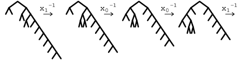
Since a tree pair diagram for will require 11 carets in each tree, we begin with a tree consisting of one caret of type and 10 carets of type . Caret is of type and is identical to the caret of . To create caret , we apply . To create caret , we apply . Caret is more complicated. We begin with , and then must traverse the right subtree of caret , which in this case is the single caret numbered . Since caret is of type , it requires only the generator . We now return to complete the sequence of generators necessary to create caret , namely . Caret , the root caret, is of type and requires only the generator . Caret is again more complicated, since it is of type . We begin with an before descending into the right subtree of caret , i.e. caret , which is created via an . we then finish the creation of caret with the string . To create caret , we apply and begin to traverse the right subtree of caret . For caret , we apply the generator and begin to traverse the right subtree of caret . Caret is created with a single generator, and caret is simply the last caret from the initial tree and requires no additional generators. We then return to finish the creation of caret by applying to make it once again a right caret, and we apply another generator to finish creating caret . Thus we have produced the tree representing and found the string
to be a minimal representative for .
This entire process is illustrated in Figure 9, and described in more detail in the following four figures.




We now prove theorem 6.1.
Proof.
We first prove that the nested traversal method produces the correct tree for strictly negative words in . Once this is proven, it is clear that the string of generators produced by the method is a minimal length representative, because the number of carets needed to create a caret of type is exactly the weight of the pair . We prove that the correct tree is produced via induction on the length of the normal form of a negative word . Note that the length of the normal form of is exactly , the word length in the infinite presentation .
We begin with the base case of the induction, and . We must prove that the nested traversal method produces the correct tree pair for . If then it is clear that the nested traversal method yields the correct pair of trees.
If with , it is easily checked that the tree for is of the following form: caret is of type and is followed by carets of type , a single caret of type , a single caret of type and a final caret. Creating these carets in infix order, following the nested traversal method, we begin with the tree containing a single caret, and carets of type .
According to the nested traversal method, we apply , which moves the first carets of type to the left side of the tree. Each of these generators is the first half of the pair of generators needed for creating an or an caret. Now, we create the caret by applying the generator ; this creates an caret with exposed leaves numbered and . We finish with , which moves all but the initial caret on the left side of the tree back to the right side of the tree. Thus, the nested traversal method, with the correct nesting, produced the tree representing the element .
We complete the proof by induction on the size of the negative word. We assume inductively that the nested traversal method produces the correct tree for a negative word with tree pair diagram . We consider a new word in normal form whose length (in the infinite presentation) is one more than the length of . If , we prove by induction that can be constructed via the nested traversal method. We divide the proof into two cases:
- (1)
in case , we assume that the normal form of begins with , and
- (2)
in case , we assume that the normal form of does not begin with .
In both cases, the tree has at least one more caret than the tree .
Case 1. Let in normal form, and thus in normal form. In terms of tree pair diagrams, let and . Let be the string of letters obtained via the nested traversal method which creates the tree , according to the induction hypothesis. We will obtain a string which is a minimal representative of and creates the tree .
- (1)
If , it is clear that the nested traversal method produces the correct tree and gives a minimal length representative for .
- (2)
Assume that . If the right subtree of the root caret of is empty (which we note can be detected via lemma 5.1) then except for the initial caret, consists entirely of left and interior carets. Since , there must be at least one interior caret in . Since constructs according to the nested traversal method, we know that can be written as , where the creates the final interior caret, which has caret number . In addition, is a sequence of letters containing at least repetitions of , which create a series of left carets in : the left carets with caret numbers greater than as well as the left caret with the highest caret number less than . The string may contain other letters prescribed by the nested traversal method.
From the normal form of , we know that the highest numbered left leaf in is leaf number , and it must be the exposed left leaf of a string of carets of type . None of the carets in this string can be of type ; if they were, then there would be an exposed left leaf with positive leaf exponent whose leaf number is greater than . Since is the largest index of a generator in the normal form of , such an caret cannot occur in this string of carets.
Such a string of carets is created according to the nested traversal method via a string of letters. Thus we can further enumerate as . Since the normal form of simply contains one more occurrence of the generator , we know that in , the exposed leaf numbered is the left exposed leaf of a sequence of carets of type . Thus the tree is created by the string of letters . Since the generator is what the nested traversal method determines will create an caret, we see that is the string produced by the nested traversal method which generates .
- (3)
Now suppose that the right caret of the root of is not empty. In this case, can be written as , where accounts for the right carets that are created in a nested manner. It is easy to see that as above, the tree is produced from the string , which is exactly the string of letters produced by the nested traversal method to generate .
Case 2. We now assume that in normal form, and that the generator does not appear in the normal form of . In all of the subcases below, we begin with a tree containing at least one more caret than the tree used to create . Since the generator does not appear in the normal form of , in the tree , there is a caret with an exposed leaf numbered , which has leaf exponent . It may be the case that one must add carets of type to the right side of to obtain the caret with exposed leaf . However, adding these carets does not affect the normal form of the element. Again, let be the string of letters generated by the nested traversal method which creates the tree .
- (1)
First, suppose that is an interior caret, which must be of type and have an exposed right leaf numbered in order for the leaf exponent of to be . Since is larger than any index of a generator in the normal form of , it also follows that the highest index appearing in the normal form of is at most .
We can write , where is the letter in which creates the caret from a right caret. It is easily seen that in , the caret becomes an caret, the leaf exponent of is now , and no new carets with higher numbered leaves and positive leaf exponent are added, which might cause additional generators to appear in the normal form for . We have exactly added the sequence of generators corresponding to an caret in the chart above describing the nested traversal method.
- (2)
Now suppose that is a left caret with an exposed right leaf numbered . Write where is the letter in which creates the caret according to the nested traversal method. Then in the tree created from by the string , the right child of the root caret has a left subtree consisting of a single caret with exposed leaves numbered and . Then, in the tree corresponding to the string , we have created the left caret whose right subtree contains a single caret, with exposed leaves numbered and . Thus the leaf exponent of is now , and so appears in the normal form of the element. Since the trees and differ only in this one place, we see that the string creates the tree . The trees and differ in a single caret, and and differ only in the generator , which is the letter that the nested traversal method uses to create an caret, we see that is the string produced by this method for the tree .
- (3)
Finally, suppose that is a right caret in with exposed left leaf , with leaf exponent . The must be a caret of type ; if it was not, then would be smaller than the index of some generator appearing in the normal form of , contradicting initial assumptions.
Since is a negative word, it contains a single caret of type which has a single right exposed leaf numbered . If there was a caret of type with two exposed leaves, the pair could be reduced. It is necessary to add a string of additional carets to the original tree in order to obtain .
Let , where is the highest index of a generator appearing in the normal form of , so in particular . It now follows that the string creates the tree . The first letters move the new carets to the left side of the tree, the creates an interior caret with exposed leaves labelled and , and the letters move the carets back to the right side of the tree where they become of type or . So again we see that the additional letters needed exactly coincide with the letters prescribed by the nested traversal method for constructing .
If we begin with a strictly positive word , we use the nested traversal method to construct a minimal length representative for the strictly negative word . The inverse of this path will then produce a minimal length representative for . ∎
The authors would like to thank Azer Akhmedov for helpful comments on an earlier draft.
References
- [1] K. S. Brown and R. Geoghegan. An infinite-dimensional torsion-free group. Inventiones mathematicae, 77:367–381, 1984.
- [2] J. Burillo, S. Cleary, and M. I. Stein. Metrics and embeddings of generalizations of Thompson’s group . Trans. Amer. Math. Soc., 353(4):1677–1689 (electronic), 2001.
- [3] José Burillo. Quasi-isometrically embedded subgroups of Thompson’s group . J. Algebra, 212(1):65–78, 1999.
- [4] J. W. Cannon, W. J. Floyd, and W. R. Parry. Introductory notes on Richard Thompson’s groups. L’Ens. Math., 42:215–256, 1996.
- [5] Sean Cleary and Jennifer Taback. Thompson’s group is not almost convex. preprint.
- [6] Blake Fordham. Minimal Length Elements of Thompson’s group . PhD thesis, Brigham Young Univ, 1995.
Sean Cleary
Department of Mathematics
City College of New York
City University of New York
New York, NY 10031
E-mail: cleary@sci.ccny.cuny.edu
Jennifer Taback
Department of Mathematics and Statistics
University at Albany
Albany, NY 12222
E-mail: jtaback@math.albany.edu