General Relativistic Shock-WavesPropagating at the Speed of Light

Acknowledgements

First and foremost I would like to thank my wife, Monika. Without her support and encouragement it is difficult to imagine completing this dissertation. I also owe a great deal to my thesis advisor Professor Blake Temple. Besides giving his support and encouragement, I have also benefitted greatly from his influence on my approach to research mathematics, and I look forward to working with him in the future.

It has been a long road for me to get to this point in my career, and I am certain I would not have made it this far without the patience, and support of my parents, Richard and Jean Scott. I am also grateful to them for letting me pursue a career of my choosing, and offering nothing but encouragement. My only wish is that my mother were still with us to witness this accomplishment.

I would also like to thank my wife’s parents Chris and Eleni Poulos for their support throughout my time at U.C. Davis even before my wife and I were married.

Abstract

We investigate shock-wave solutions of the Einstein equations in the case when the speed of propagation is equal to the speed of light. The work extends the shock matching theory of Smoller and Temple to the lightlike case. After a brief introduction to general relativity, we introduce a previously known generalization of the second fundamental form by Barrabès and Israel. Then we use this to develop an extension of a shock matching theory, which characterizes solutions of the Einstein equations when the spacetime metric is only Lipschitz continuous across a hypersurface, to include the case when the hypersurface is lightlike. The theory also demonstrates an unexpected result that the matching of the generalized second fundamental form alone is not a sufficient condition for conservation conditions to hold across the interface. Using this theory we then construct a new exact solution of the Einstein equations that can be interpreted as an outgoing spherical shock wave that propagates at the speed of light. This is done by matching a Friedman Robertson Walker (FRW) metric, which is a geometric model for the universe, to a Tolman Oppenheimer Volkoff (TOV) metric, which models a static isothermal spacetime. Then our theory is used to show that the matched FRW, TOV metric is a solution. The pressure and density are finite on each side of the shock throughout the solution, the sound speeds, on each side of the shock, are constant and subluminous. Moreover, the pressure and density are smaller at the leading edge of the shock which is consistent with the Lax entropy condition in classical gas dynamics. However, the shock speed is greater than all the characteristic speeds. The solution also yields a surprising result in that the solution is not equal to the limit of previously known subluminous solutions as they tend to the speed of light.

Notation and Conventions

$R^{\mu}_{\hskip 4.0pt\alpha\nu\beta}$ denotes the Riemann curvature tensor.

$R_{\alpha\beta}=R^{\mu}_{\hskip 4.0pt\alpha\mu\beta}$ denotes the Ricci curvature tensor.

$R=g^{\alpha\beta}R_{\alpha\beta}$ denotes the Ricci scalar.

$G$ , $G_{\alpha\beta}=R_{\alpha\beta}-(1/2)g_{\alpha\beta}R$ denotes the Einstein curvature tensor.

$M$ denotes the $n$ - or four-dimensional spacetime manifold.

$\Sigma$ denotes a hyper- or shock-surface in $n$ - or four-dimensional spacetime.

$T_{p}\Sigma$ denotes the tangent space of $\Sigma$ at a point $p$ in $\Sigma$ .

$T_{p}M$ denotes the tangent space at $p$ in the spacetime manifold $M$ .

$X_{a}$ denotes a basis vector of $T_{p}\Sigma$ .

$X$ denotes a tangent vector in $T_{p}\Sigma$ .

$\mathbf{n}$ denotes the vector normal to $T_{p}\Sigma$

$\mathbf{N}$ denotes a vector transverse to $\Sigma$ , which cannot be in $T_{p}\Sigma$ .

$[\,\cdot\,]$ denotes the jump in a quantity across $\Sigma$ . For example, $[g(p)]=g^{L}(p)-g^{R}(p)$ for $p$ in $\Sigma$ where $g=g^{L}$ on the left side of $\Sigma$ , and $g=g^{R}$ on the right side of $\Sigma$ .

$K(X)=-\nabla_{X}\mathbf{n}$ denotes the second fundamental form.

$\mathcal{K}(X)=-\nabla_{X}\mathbf{N}$ denotes a generalized second fundamental form which depends $\mathbf{N}$ .

$C^{k}$ denotes a function which is at least $k$ times differentiable and it $k$ th derivative is continuous.

$C^{k,1}$ is a $C^{k}$ function whose $k$ th derivative is Lipschitz continuous.

$\mbox{diag}(-1,1,\ldots,1)$ denotes an $n\times n$ diagonal matrix with the first entry equal to $-1$ and the remaining non-zero entries equal to $1$ .

Notation for derivatives: For partial derivatives $\partial F/\partial x^{a}=F_{,a}$ . For covariant derivatives $\nabla_{a}F=F_{;a}.$

Chapter 1 Introduction

In this dissertation we give a general theory of shock matching in the lightlike case, and use this theory to construct a new exact solution of the Einstein equations that can be interpreted as an outgoing spherical shock wave that propagates at the speed of light. The general theory extends the shock matching theory of Smoller and Temple [14, 15] to the case of lightlike interfaces. Based on this new theory we construct our exact solution by matching an Friedman Robertson Walker (FRW) metric to a Tolman Oppenheimer Volkoff (TOV) metric across an outgoing radial, lightlike shock wave. In this exact solution matter crosses the interface, but nothing propagates at the speed of light except the shock wave. As far as we know this is the first such exact solution in general relativity.

In this exact solution the shock wave emerges from the FRW origin at the instant of the Big Bang, and propagates all the way out to infinity. The pressure and density are finite on each side of the shock throughout the solution, the sound speeds, on each side of the shock, are constant and subluminous. Moreover, the pressure and density are smaller at the leading edge of the shock which is consistent with the entropy condition in classical gas dynamics [7]. However, the shock speed is greater than all the characteristic speeds, see [15]. Subluminous shocks with this characteristic condition were constructed in [15].

In the general theory we translate generalized notion of the second fundamental form of Barrabès and Israel [1] into the shock matching framework of Smoller and Temple [14, 15]. We base the analysis on a modified Gaussian Skew (MGS) coordinate system on lightlike surfaces which we introduce in this dissertation.

One surprise is that the relation between the sound speeds on the front and back sides of the shock in our new exact solution, are not equal to the speeds in the limit as the shock speed in the Smoller-Temple solutions, obtained in [15], tend to the speed of light.

Another surprise is that the general theory shows there exist gravitational metric components which are $C^{1,1}$ across a lightlike surface for which $\mbox{div}\,G=0$ does not hold in the weak sense. This implies that the matching of the (generalized) second fundamental form alone is not a sufficient condition for conservation conditions to hold across the interface.

1.1. The Central Problem: Lightlike Shock-Waves

The goal of the work here is to construct shock-wave solutions of the Einstein equations which move at the speed of light. In Einstein’s general relativity all physically possible spacetimes correspond to solutions of Einstein’s Equations

(1.1)

G=\kappa T,

which are metrics that describe the geometric structure of spacetime. Equation (1.1) is a tensor equation representing 10 nonlinear partial differential equations where $G$ describes the geometric structure of spacetime, and $T$ represents the matter which is the source of the gravitational field.

Shock-waves were first studied in compressible, non-viscous gas flow as discontinuities that form in the fluid quantities pressure, density, etc. The mathematical theory of shock-waves is contained in the study of hyperbolic conservation laws, and applies to much more that just gas dynamics. Mathematical shock wave theory not only models phenomena such as the sonic boom created by a fast moving plane, but the same theory also incorporates the propagation of “gridlock” in traffic flow, the leading edge of a nuclear explosion, flame fronts in combustion, and separation of boundaries between chemical species in chromatography [17]. If we take the covariant divergence of equation (1.1), then it turns out that

(1.2)

\mbox{div}\,T=0.

In the limit of low velocities and weak gravitational fields equation (1.2) reduces to the classical compressible Euler equations which is a hyperbolic conservation law in gas dynamics.

The shock-wave solutions considered in this dissertation are constructed by matching two metrics (geometries) across a surface embedded in spacetime. In their well-known 1939 paper [11] describing gravitational collapse of a star, Oppenheimer and Snyder gave the first example, which had interesting dynamics, of a solution of the Einstein equations obtained by matching two solutions across a surface [14]. With their simplifying assumption that the pressure is zero, the surface across which the metrics are matched is not shock-wave, but a contact discontinuity which is a discontinuous solution where neither mass or momentum cross [14]. Smoller and Temple extended the Oppenheimer-Snyder model of gravitational collapse to the case of non-zero pressure in their 1994 paper [14]. Their theory was based on work done by Israel in his 1966 paper [6], which related the second fundamental form across a shock surface to the Rankine-Hugoniot jump conditions across the shock. Then, in later work [15], Smoller and Temple constructed a family of exact, spherically symmetric, shock-wave solutions of the Einstein equations by matching two spherically symmetric metric across a surface. The shock surfaces in Smoller and Temple’s work are assumed to be non-lightlike, that is, moving slower than the speed of light. The contribution here will be to extend their results given in [14] and [15] to also incorporate the case when the surface is lightlike.

The Two Difficulties of the Lightlike Case

In the lightlike case the mathematical machinery used in the sub-luminal case breaks down in two areas. First, the induced metric on a lightlike surface is degenerate, and the second is that the second fundamental form,

(1.3)

K=-\nabla_{X}\mathbf{n},

cannot be used to describe the dynamics of the surface in the ambient spacetime. A lightlike surface is characterized by the length of the normal vector being zero. Note the in this case the normal vector is non-zero, but the metric is not positive definite. A normal of zero length is orthogonal to itself, hence it lies in the tangent space of the surface. Since the normal is no longer transverse to the surface, the second fundamental form no longer gives information about how the surface in embedded in the spacetime manifold.

The degeneracy problem is dealt with by considering the problem in the context of the whole spacetime manifold where the metric is not degenerate. Unfortunately, the failure of the second form is not fixed so easily. To rectify this failure we make use of an idea originated by Barrabès and Israel in [1] in which they define a generalized second fundamental form in terms of a vector $\mathbf{N}$ transverse to the surface.

The work of Barrabès and Israel in [1] focuses on the dynamics of surface layers whose theory is also based on matching two metrics across a surface. A surface layer differs from a shock-wave in that a shock surface is characterized by a jump in the density of the fluid across the surface, in contrast, the density becomes infinite in a surface layer. Mathematically, the Einstein tensor $G$ , which comprises the right hand side of equation (1.1), contains no delta-function singularities across a shock surface, but across a surface layer $G$ does contain a delta-function singularity. We also note here that Barrabès and Israel use a scalar version of the second fundamental form where we use the form given in equation (1.3) which is a tangent vector in the surface. Regarding the lightlike case, Barrabès and Israel state that because of the breakdown in the second fundamental form, the lightlike case is a relatively neglected area of surface dynamics which remains imperfectly understood [1].

1.2. How This Document is Organized

In chapter 2 we give an introduction to general relativity, and a derivation of the second fundamental form. Then in chapter 3 we give a generalization of the second fundamental form based on the idea of using a transverse vector in place of the normal vector. Continuing on, we state and prove the main result of this dissertation giving a set of equivalent conditions which yield the existence of shock solutions in the Einstein equations when the metric is Lipschitz continuous across a hypersurface, and we finish the chapter by proving a similar result involving spherically symmetric metrics. In chapter 4 we give an exact, spherically symmetric, lightlike shock-wave solution of the Einstein equations based on Smoller and Temple’s work in [15]. Chapter 5 concludes the results.

Chapter 2 General Relativity and the Second Fundamental Form

The purpose of this chapter is to make this dissertation self-contained for anyone with a good understanding of differential geometry. We construct the geometry of spacetime from physical assumptions, derive the stress-energy tensor for a perfect fluid, define the Einstein equations, and conclude the chapter with an introduction of the second fundamental form.

The underlying theme of general relativity is the idea that the physics of our universe and its geometry are interdependent in such a way that they cannot be separated from each other. The Einstein field equations,

G=\kappa T,

is a mathematical formulation of this idea with respect to the physics of gravity. The Einstein equations match $G$ , a second order differential operator on the metric that is related to the Riemannian curvature tensor, to $T$ , the stress-energy tensor of the fluid or matter in the region of spacetime that is being considered.

2.1. The Geometry of Spacetime

A theory of gravitation begins with a notion of space and time. Spacetime is a continuum of events each of which has three spacial components, and one time component. If we give each event a name in terms of these components, say $x=(x^{0},x^{1},x^{2},x^{3})$ where $x^{0}=ct$ with $c$ the speed of light in a vacuum, $t$ denoting time, and $x^{a}$ for $a=1,2,3$ representing the spacial components, then we can represent each event in as a coordinate $x$ . The geometry of spacetime is the structure of how this continuum of events fit together. We shall see, it is the principles from physics that will determine this structure.

Mathematically spacetime is a four dimensional manifold $M$ equipped with a metric $g$ . It is the metric that carries the information about the rates at which clocks run, and the distances between points. It is also the metric that describes the geometry. The question now is how do we determine a metric which models spacetime or subset of it?

Special Relativity

In order to proceed we need the notion of an inertial coordinate frame or sometimes called an inertial observer. A coordinate system is inertial if any two events in the coordinate system share the same clock or time coordinate, and the geometry of space at any constant time is Euclidean [12]. Consider a spacetime without gravity, that is, a spacetime containing negligible mass. This is the realm of special relativity which can be deduced by the two following postulates:

Postulate 1 (Principle of Relativity).

Let $x$ be an inertial coordinate system. Then any other coordinate system $\bar{x}$ which moves uniformly, and is non-rotating relative to $x$ is also an inertial coordinate system. Furthermore, ”The laws of nature are in concordance for all inertial systems”[2].

Postulate 2 (Propagation of light).

The speed of light in a vacuum $c$ is observed to be the same from any inertial coordinate system.

The principle of relativity is equivalent to the statement that any body in uniform motion remains in that state unless acted upon by an external force [12]. The universality of the speed of light means that two observers, one moving with non-zero uniform velocity with respect to the other, will each observe a single light ray moving through vacuum to be travelling at same speed $c$ .

Measuring Distance in a Special Relativistic Spacetime

Consider two inertial frames $O$ and $\bar{O}$ , each having only one spatial dimension for simplicity, with coordinates $(x,ct)$ , and $(\bar{x},c\bar{t})$ respectively. Assume $\bar{O}$ is moving along the $x$ axis with relative uniform velocity $v$ see figure 2.1.

Let two events be connected by a light ray. Then in the $O$ frame the squared distance between the events is given by

(2.1)

\Delta s^{2}=-(\Delta ct)^{2}+(\Delta x)^{2}=0.

By the propagation of light law the same two events, in the $\bar{O}$ frame , also satisfy

(2.2)

\Delta\bar{s}^{2}=-(\Delta c\bar{t})^{2}+(\Delta\bar{x})^{2}=0.

Now, assume that coordinate transformation from $O$ to $\bar{O}$ is linear, and that their origins coincide. Then if follows that

\Delta s^{2}=\Delta\bar{s}^{2}

for any two events in spacetime for any inertial coordinate frames $O$ and $\bar{O}$ whose origins coincide, and are related by a linear transformation.

Recall that the metric $g$ is required to give data on the rates at which clocks run, and the distances between spatial points. Since any data determined by the metric also needs to satisfy postulate 1, we require that $g$ be a coordinate independent quantity. Therefore, $g$ should incorporate the coordinate invariant quantity $\Delta s^{2},$ which composed of squared displacements between events.

What is the formula for $g$ in a given inertial frame? Let $\vec{A}$ denote a displacement vector between two events in some inertial coordinate system. Then the squared distance between the two events in the coordinates is given by

g(\vec{A},\vec{A})=-(A^{0})^{2}+(A^{1})^{2}+(A^{2})^{2}+(A^{3})^{2},

which consistent with the squared distance in (2.2). This leads to the inner product between any two vectors $\vec{A}$ , and $\vec{B}$ given by

g(\vec{A},\vec{B})=-A^{0}B^{0}+A^{1}B^{1}+A^{2}B^{2}+A^{3}B^{3}.

Notice this is very similar to the standard dot product with the only difference being the negative sign on the product of the first components. We can also write this metric in the following form:

(2.3)

g(\vec{A},\vec{B})=\begin{pmatrix}A^{0}\\ A^{1}\\ A^{2}\\ A^{3}\end{pmatrix}^{T}\begin{pmatrix}-1&0&0&0\\ 0&1&0&0\\ 0&0&1&0\\ 0&0&0&1\end{pmatrix}\begin{pmatrix}B^{0}\\ B^{1}\\ B^{2}\\ B^{3}\end{pmatrix}.

In this form we can see that $g$ has a signature of $+2$ . A metric with this signature is said to have a Lorentzian signature. We will only deal with metrics of Lorentzian signature. Furthermore, the metric given in (2.3) is said to be Minkowskian, and is denoted by $\eta_{\alpha\beta}=\mbox{diag}(-1,1,1,1)$ . The inner product $g$ is not positive definite. To see this consider

g(\vec{A},\vec{A})=\langle(1,1,0,0),(1,1,0,0)\rangle=-1+1=0.

However, we can always find a coordinate basis so that $g$ is of the form $\eta_{\alpha\beta}$ . Therefore $g$ is non-degenerate, that is, $g(\vec{A},\vec{B})=0$ for all vectors $\vec{B}$ if and only if $\vec{A}=0$ .

Definition 2.1.

A vector $\vec{A}$ is said to be spacelike if $g(\vec{A},\vec{A})>0,$ is lightlike if $g(\vec{A},\vec{A})=0$ , is timelike if $g(\vec{A},\vec{A})<0$ .

From this we can give the causal structure of spacetime, that is the causal relationship of an event to other events. The future or past of an event $p$ lies inside the light cone of $p$ , see figure 2.2. If an event $p$ lies at the origin of an inertial frame, then the future and past of $p$ is given by all events $q$ such that the displacement vectors between $p$ and $q$ are timelike.

Summary 2.2 (Special Relativity).

From postulates 1 and 2 we were able to describe how the squared distance $\Delta s^{2}$ should be measured, and that it is invariant under coordinate transformations between inertial frames. From the idea of $\Delta s^{2}$ we defined the inner product $g$ given in (2.3), and designated it as our metric for spacetime with no gravity. From this we ascertained that $g$ is a metric with Lorentzian signature.

General Relativity

We now consider spacetime with gravity. We are motivated by the fact that objects under the influence of gravity move along free fall paths. To see this imagine an observer in a spaceship with the engines turned off, and orbiting the earth under the influence of only earth’s gravity at a distance $r_{0}$ above the earth. We are assume the earth is a perfect uniform sphere, and ignoring the fact that the earth is rotating. Then an observer inside the spacecraft now feels weightless, and can position themselves in such way that they remain stationary in the middle of the ship so that they are not moving relative to the walls of the ship. The ship, and the observer are moving along a free fall path of earth’s gravity. Such a coordinate frame is said to be comoving with the metric.

How does the observer know that they are under the influence of a gravitational force? Consider a second ship in orbit the same distance $r_{0}$ above earth, but positioned a distance $d$ to the right. Also, assume the second ship is moving with the same velocity parallel to the original ship at some instant of time say $t_{0}$ , see figure 2.3.

As seen in figure 2.3, the distances between the two ships is not constant, and their paths will even cross. In this space Euclid’s parallel axiom does hold, and spacetime is curved.

Mathematically, for the local coordinate system, (inside the original ship) the Minkowskian metric, $g_{\alpha\beta}=\eta_{\alpha\beta}$ , is appropriate just as it was in special relativity. Also, at the point of spacetime where the ship is located, we have $g_{\alpha\beta,\gamma}=0$ . This defines a locally inertial frame or also called locally Lorentzian.

A logical question to ask at this point is, does there exist a global inertial frame when gravity is present? The answer is no. We have already seen from our example that the two ships cannot be described by the same inertial frame because they lie in a curved space which is not Euclidean in it’s spatial components violating the definition of an inertial frame. This violation is due to the non-uniformity of the earth’s gravitational field. As we expect with a curved space, we can only consider local frames diffeomorphic to $\mathbb{R}^{4}$ .

The idea that objects moving in a gravitational field are described by comoving local inertial systems takes into account the Equivalence Principle. The Equivalence Principle says that all bodies move the same way in a gravitational field [18]. It is the equivalence principle that motivated Einstein to formulate the theory of general relativity.

The implication that under the influence of gravity particles move in a curved space, which can only be described in the context of locally inertial frames, is that we have to use the mathematical machinery of differential geometry to characterize the dynamics of particles under the influence of gravity. This is in contrast to special relativity where the curvature is zero, since their is no acceleration of particles due to gravity, and one coordinate frame is sufficient to describe spacetime. Therefore, we will present the concepts from differential geometry that are needed to describe a curved spacetime.

The Metric in a Curved Spacetime

The metric completely defines the curvature of the spacetime manifold, and so we begin by constructing the spacetime metric $g$ for a possibly curved spacetime. Earlier we used displacement vectors to construct the Minkowski metric in the flat spacetime of special relativity. If the displacements are infinitesimally small, then we can associate them with tangent vectors, which are defined by directional derivatives. Let $p$ be in a point in the spacetime manifold $M$ , and suppose

x=(x^{0},x^{1},x^{3},x^{3}):M\longrightarrow\mathbb{R}^{4},

are coordinates on $M$ whose origin is at $p$ , where $x^{0}=ct$ , $c=1$ , and $x^{i}$ for $i=1,2,3$ denote the spatial coordinates. Also let $\mathcal{F}$ denote the set of all $C^{\infty}$ functions that take smooth curves on $M$ into $\mathbb{R}$ .

(2.4)

\begin{CD}M@<{x^{-1}}<{}<\mathbb{R}^{4}\\ @V{f}V{}V\\ \mathbb{R}\end{CD}

Then a tangent vector $X$ at $p$ in $M$ is defined to be a map $X:\mathcal{F}\to\mathbb{R}$ . For any coordinate system $x$ on a neighborhood of $p$ , there exist a coordinate basis given by

(2.5)

X_{\alpha}\left(f(p)\right)=\left.\frac{\partial}{\partial x^{\alpha}}(f\circ x^{-1})\right|_{x(p)}.

See diagram in (2.4). That is, $\{\partial/\partial x^{\alpha}\}$ gives a basis for $T_{p}M$ , the tangent space of $M$ at $p$ .

We now introduce the Einstein summation convention which says that for any expression, equal up and down indices are summed over all possible values the index can take. For example, using (2.5), if $X\in T_{p}M$ , then

X=\sum_{\alpha=0}^{3}X^{\alpha}\frac{\partial}{\partial x^{\alpha}}=X^{\alpha}\frac{\partial}{\partial x^{\alpha}}.

Notice that the upper index in the denominator is considered a down index.

With tangent vectors defined as directional derivatives, they are in one-to-one correspondence with displacement vectors. Since the metric is quadratic in displacements we define $g$ as a map where

g:T_{p}M\times T_{p}M\longrightarrow\mathbb{R}.

Also, we assume that $g$ is symmetric, and non-degenerate as was the case in special relativity.

The metric $g$ being symmetric guarantees, that in coordinates, the components of the metric $g_{\alpha\beta}$ make up a symmetric matrix, and therefore there will always exist a linear transformation to another coordinate system that will take $g_{\alpha\beta}$ to $\eta_{\alpha\beta}=\mbox{diag}(-1,1,1,1),$ the Minkowski metric. Furthermore, it can also be shown that the metric $g$ is locally Lorentzian or locally inertial, that is, given $p$ in $M$ , there exist coordinates $x$ whose origin is at $p$ such that

g_{\alpha\beta}(p)=\eta_{\alpha\beta}\quad\mbox{for}\quad\alpha,\beta=0,1,2,3,

g_{\alpha\beta,\mu}(p)=0\quad\mbox{for}\quad\alpha,\beta,\gamma=0,1,2,3,

and

g_{\alpha\beta,\mu\nu}(p)\neq 0,

at the point $p$ for at least some values of $\alpha,$ $\beta$ , $\mu$ and $\nu$ if spacetime is not flat, that is, there exists a gravitational field. This corresponds exactly with the notion of locally inertial frames given in the previous section.

Tensors in Spacetime

An alternative version of the Equivalence Principle is the General Covariance Principle which motivates the use of tensors to measure physical quantities that depend linearly on displacements. The General Covariance Principle states that an equation holds in a gravitational field if the two following conditions are met [20]:

(1)

The equation holds in the absence of a gravitational field; that is, it is consistent with postulates 1 and 2.
(2)

The equation is covariant, which means that the equation holds under any coordinate transformation $x\to y$ .

We take the following definition of a tensor from [18]. Given a finite vector space $V$ , and denoting its dual space by $V^{*}$ , a tensor, T, of type $(k,l)$ on the space $V$ is a multilinear map

(2.6)

T:(V^{*})^{k}\times V^{l}\longrightarrow\mathbb{R}.

Note that our definition of tensor makes no mention vector or dual vector components. A tensor gives the same real number for a particular set of vectors and dual vectors independent of the coordinates the components are computed in.

Our first example of a tensor is the metric $g$ which is a $(0,2)$ tensor, that can be written in terms of coordinate basis one-forms as

(2.7)

ds^{2}=g_{\alpha\beta}\,dx^{\alpha}\otimes dx^{\beta}=g_{\alpha\beta}\,dx^{\alpha}dx^{\beta}.

It is customary to drop the exterior product sign between the one-forms $dx^{\alpha}$ . Furthermore, the metric provides a mapping between vectors and one-forms (dual vectors) at every point. Thus, given a vector field $X(p)$ , there is a unique one-form field given by $\tilde{X}(p)=g(X(p),\quad)$ .

Using this map between vectors and one-forms we can construct a unique and useful one-form basis. Suppose $\{\partial/\partial x^{\alpha}\}$ is a coordinate basis for $T_{p}M$ . Then $\{dx^{\alpha}\equiv g(\partial/\partial x^{\alpha},\quad)\}$ gives a one-form basis.

Since $g$ is non-degenerate, there exists an inverse which takes one-forms to vectors. If the indices of the basis one-forms are ‘‘up” and ‘‘down” for basis vectors, then we can use the Einstein summation convection to keep track of these mappings. Notice that for the Einstein summation convention to work we have to have the indices of vector components “up,” and the indices on components of the one-forms “down.” For example, see equation (2.7). The components for the inverse of $g$ are denoted by $g^{\alpha\beta}$ . Notice that $g_{\alpha\sigma}g^{\sigma\beta}=\delta_{\alpha}^{\beta}$ as we would expect from matrix multiplication. Using the metric $g$ as an invertible map from vectors to one-forms can be executed by raising and lowering an index of a tensor by contracting the index with metric. For example, we can map the vector $X$ to a one-form as

g_{\alpha\sigma}X^{\sigma}=X_{\alpha}.

Another example mapping a $(3,1)$ tensor to a $(2,2)$ tensor:

g^{\beta\sigma}R^{\alpha}_{\sigma\mu\nu}=R^{\alpha\beta}_{\mu\nu}.

The components of a $(k,l)$ tensor given in one coordinate system can be written in terms of another set of coordinate system via the tensor transformation law:

(2.8)

T^{\alpha_{1},...,\alpha_{k}}_{\beta_{1},...,\beta_{l}}=T^{\mu_{1},...,\mu_{k}}_{\nu_{1},...,\nu_{l}}\frac{\partial y^{\alpha_{1}}}{\partial x^{\mu_{1}}}\cdots\frac{\partial y^{\alpha_{k}}}{\partial x^{\mu_{k}}}\frac{\partial x^{\nu_{1}}}{\partial y^{\beta_{1}}}\cdots\frac{\partial x^{\nu_{l}}}{\partial y^{\beta_{l}}}.

Here we have written a $y$ -coordinate tensor component $T^{\alpha_{1},...,\alpha_{k}}_{\beta_{1},...,\beta_{l}}$ in terms of $x$ -coordinates. Also, note that the Jacobian matrix satisfies $\frac{\partial x}{\partial y}=\left(\frac{\partial y}{\partial x}\right)^{-1}.$

Parallel Transport and the Derivative Operator

Motivated by the idea of describing the curvature of spacetime intrinsically, as opposed to describing spacetime as an embedding in some other space, we will define curvature in terms of parallel transport. Intuitively, a vector field $Y$ defined on every point along a curve is said to be parallel transported along the curve if the vectors of $Y$ are parallel, and are of equal length at infinitesimally close points. Mathematically, in a locally Lorentzian frame at a point $p$ , the components of the $Y$ vectors must stay constant along the curve near $p$ . If we let $x(\xi)$ be a parameterization of the said curve, and denote the its tangent by $X=dx/d\xi,$ then $dY^{\alpha}/d\xi=0$ at $p$ . However,

(2.9)

\frac{dY^{\alpha}}{d\xi}=\frac{dx}{d\xi}\frac{dY^{\alpha}}{dx}=X^{\beta}\frac{\partial Y^{\alpha}}{\partial x^{\beta}}=0.

Equation (2.9) leads to the idea that in order to define parallel transport for any coordinate frame, not just an locally inertial system, we require a notion of how to take derivatives of vector fields.

Consider the vector field $Y$ in an arbitrary coordinate frame, not necessarily Lorentzian. We differentiate $Y$ as follows:

(2.10)

\nabla_{\beta}Y\equiv\frac{\partial}{\partial x^{\beta}}\left(Y^{\alpha}\frac{\partial}{\partial x^{\alpha}}\right)=\frac{\partial Y^{\alpha}}{\partial x^{\beta}}\frac{\partial}{\partial x^{\alpha}}+Y^{\alpha}\frac{\partial}{\partial x^{\beta}}\frac{\partial}{\partial x^{\alpha}}.

Now,

\frac{\partial}{\partial x^{\beta}}\frac{\partial}{\partial x^{\alpha}}

is a vector and can be written in terms of the coordinate basis, that is,

(2.11)

\frac{\partial}{\partial x^{\beta}}\frac{\partial}{\partial x^{\alpha}}=\Gamma^{\mu}_{\alpha\beta}\frac{\partial}{\partial x^{\mu}},

where $\Gamma^{\mu}_{\alpha\beta}$ is called a Christoffel symbol which is yet to be determined. Therefore, we can write equation (2.10) as

(2.12)

\nabla_{\beta}Y\equiv Y_{;\beta}=\frac{\partial Y^{\alpha}}{\partial x^{\beta}}\frac{\partial}{\partial x^{\alpha}}+Y^{\alpha}\Gamma^{\mu}_{\alpha\beta}\frac{\partial}{\partial x^{\mu}}\equiv Y^{\alpha}_{\hskip 5.0pt,\beta}\frac{\partial}{\partial x^{\alpha}}+Y^{\alpha}\Gamma^{\mu}_{\alpha\beta}\frac{\partial}{\partial x^{\mu}}.

The differential operator $\nabla$ is called the covariant derivative. Given arbitrary vector fields $X$ and $Y$ the covariant derivative is defined as

(2.13)

\nabla_{X}Y=X^{\alpha}\nabla_{\alpha}Y=X^{\alpha}Y^{\beta}_{\hskip 5.0pt;\alpha}\,\frac{\partial}{\partial x^{\beta}}.

Notice that our definition of covariant derivatives did not involve the metric. However, if we recall that the metric $g$ maps vectors into one-forms, then it would seem that the metric would have something to do with how their derivatives are related. In a locally Lorentzian coordinate frame we know that for any vector field $Y,$

Y_{,\alpha}=Y_{;\alpha},

since the derivatives of the basis vectors are zero just as in special relativity. The same relation holds true for any tensor in a Lorentzian frame including the metric. Therefore, in a locally Lorentzian frame, the covariant derivative of metric components are given by

(2.14)

g_{\alpha\beta;\gamma}=g_{\alpha\beta,\gamma}=0.

Invoking the General Covariance Principle, we find that

(2.15)

g_{\alpha\beta;\gamma}=0

holds in any coordinate frame. Using this result any Christoffel symbol can be written in terms of the metric. To do this we must first show that $\Gamma^{\sigma}_{\mu\nu}=\Gamma^{\sigma}_{\nu\mu}.$

Consider a scalar field $\phi$ in a Lorentzian coordinate frame. Then $\nabla\phi$ is a one-form with components $\phi_{,\beta}$ . In the Lorentzian frame

(2.16)

\phi_{,\alpha;\beta}=\phi_{,\alpha,\beta}=\phi_{,\beta,\alpha}=\phi_{,\beta;\alpha},

since partial derivatives commute. Once more, invoking the General Covariance Principle, we have that the symmetry in equation (2.16) holds in any coordinate system. Therefore, in any coordinate frame

\phi_{,\alpha;\beta}-\phi_{,\beta;\alpha}=\phi_{,\alpha,\beta}-\Gamma^{\sigma}_{\alpha\beta}\phi_{,\sigma}-\phi_{,\beta,\alpha}+\Gamma^{\sigma}_{\beta\alpha}\phi_{,\sigma}=0,

and we have that

(2.17)

\Gamma^{\sigma}_{\alpha\beta}=\Gamma^{\sigma}_{\beta\alpha}.

Then, since $g_{\alpha\beta;\gamma}=0$ in any coordinate system, we can write

(2.18)	$\displaystyle g_{\alpha\beta,\gamma}$	$\displaystyle=\Gamma^{\sigma}_{\alpha\gamma}g_{\sigma\beta}+\Gamma^{\sigma}_{\beta\gamma}g_{\sigma\alpha},$
	$\displaystyle g_{\gamma\alpha,\beta}$	$\displaystyle=\Gamma^{\sigma}_{\gamma\beta}g_{\sigma\alpha}+\Gamma^{\sigma}_{\alpha\beta}g_{\sigma\gamma},$
	$\displaystyle g_{\beta\gamma,\alpha}$	$\displaystyle=\Gamma^{\sigma}_{\beta\alpha}g_{\sigma\gamma}+\Gamma^{\sigma}_{\gamma\alpha}g_{\sigma\beta}.$

Thus

(2.19)

-g_{\alpha\beta,\gamma}+g_{\gamma\alpha,\beta}+g_{\beta\gamma,\alpha}\\ =-\Gamma^{\sigma}_{\alpha\gamma}g_{\sigma\beta}-\Gamma^{\sigma}_{\beta\gamma}g_{\sigma\alpha}+\Gamma^{\sigma}_{\gamma\beta}g_{\sigma\alpha}+\Gamma^{\sigma}_{\alpha\beta}g_{\sigma\gamma}+\Gamma^{\sigma}_{\beta\alpha}g_{\sigma\gamma}+\Gamma^{\sigma}_{\gamma\alpha}g_{\sigma\beta}.

Using the symmetry property (2.17), equation (2.19) the Christoffel symbol can be given in terms of the metric as

(2.20)

\Gamma^{\sigma}_{\alpha\beta}=\frac{1}{2}g^{\sigma\gamma}\{-g_{\alpha\beta,\gamma}+g_{\gamma\alpha,\beta}+g_{\beta\gamma,\alpha}\}.

Now that we have a differential operator in hand we can define parallel transport without reference to a coordinate system. This is accomplished by expressing the parallel transport condition given in equation (2.9) in a covariant way. Rewriting (2.9) as

(2.21)

X^{\beta}Y^{\alpha}_{\hskip 5.0pt,\beta}=X^{\beta}Y^{\alpha}_{\hskip 5.0pt;\beta}=0,

which holds, if and only if,

(2.22)

\nabla_{X}Y=0,

see equation (2.13). Since equation (2.22) is a tensor equation, it must hold for any coordinate system. Equation (2.22) defines parallel transport of a vector $Y$ along a curve with tangent vector $X$ . Furthermore, given any initial value of $Y$ , equation (2.22) has a unique solution, and so given any initial vector $Y$ at a point on a curve this defines a unique vector at any other point on the curve. Then we can use the structure of parallel transport to map $T_{p}M$ to $T_{q}M$ along a given curve from point $p$ to point $q$ . The covariant derivative, which gives this notion of identifying tangent spaces from different points along a curve, is also referred to as a connection, and the Christoffel symbols $\Gamma^{\sigma}_{\alpha\beta}$ are referred to as connection coefficients.

With a definition of parallel transport we are in a position to describe, mathematically, the “free fall” paths in a gravitational field. These paths correspond to the geodesics in the spacetime manifold. The geodesics of the flat spacetime in special relativity are straight lines. Qualitatively, geodesics can be thought of as the straightest lines possible in a curved manifold, and they also correspond to the “straight” lines at the origin in a Lorentzian coordinate frame. In flat manifold the straight lines are the only curve in which the tangent vector parallel transports itself. Generally, a geodesic is given by the equation

(2.23)

\nabla_{X}X=0,

which finds the curves where the tangent vectors parallel transport themselves. If we let $\xi$ be a parameter which gets mapped to curve, then

X^{\alpha}_{\hskip 5.0pt,\beta}=\frac{dx^{\beta}}{d\xi}\frac{\partial\;}{\partial x^{\beta}}=\frac{d}{d\xi},

and we can write the geodesic equation (2.23) as

(2.24)

\frac{d}{d\xi}\left(\frac{dx^{\alpha}}{d\xi}\right)+\Gamma^{\alpha}_{\sigma\beta}\frac{dx^{\sigma}}{d\xi}\frac{dx^{\beta}}{d\xi}=0,

which is a second order quasi-linear differential equation for $x^{\alpha}(\xi)$ . Equation (2.24) has a unique solution given an initial position $x^{\alpha}_{0}=x(\xi_{0})$ , and an initial direction $X^{\alpha}_{0}=X^{\alpha}(\xi_{0})$ at $\xi_{0}$ [12]. This idea will be used in chapter 3, that is, we will be given a point in spacetime and vector at that the point, and be able to define a unique geodesic through the point.

The Curvature Tensor

Having defined parallel transport we are now able to define curvature. The Riemann Curvature Tensor describes the failure of initially parallel geodesics to remain parallel [18]. This corresponds to the situation involving the spacecraft orbiting earth in figure 2.3.

If we parallel transport a vector $X$ around a coordinate grid loop starting and ending at point $A$ in figure (2.4),

then it can be shown, using the general coordinates $x^{\alpha}$ and $x^{\beta}$ , the change of $X^{\gamma}$ by parallel transport along $\Delta a\,\partial/\partial x^{\alpha}$ , then $\Delta b\,\partial/\partial x^{\beta}$ , then $-\Delta a\,\partial/\partial x^{\alpha},$ and back to $A$ along $\Delta b\,\partial/\partial x^{\beta}$ is given by

\Delta X^{\gamma}=\Delta a\Delta b\left(\Gamma^{\gamma}_{\mu\alpha,\beta}-\Gamma^{\gamma}_{\mu\beta,\alpha}+\Gamma^{\gamma}_{\sigma\beta}\Gamma^{\sigma}_{\mu\alpha}-\Gamma^{\gamma}_{\sigma\alpha}\Gamma^{\sigma}_{\mu\beta}\right)X^{\mu},

see [12, section 6.5]. From this comes the definition of the Riemann curvature tensor:

(2.25)

R^{\mu}_{\hskip 4.0pt\alpha\nu\beta}=\Gamma^{\mu}_{\alpha\beta,\nu}-\Gamma^{\mu}_{\alpha\nu,\beta}+\Gamma^{\mu}_{\sigma\nu}\Gamma^{\sigma}_{\alpha\beta}-\Gamma^{\mu}_{\sigma\beta}\Gamma^{\sigma}_{\alpha\nu}.

The Riemann curvature tensor $R^{\mu}_{\hskip 4.0pt\alpha\nu\beta}$ transforms as tensor, via the tensor transformation law (2.8), giving a covariant measure of the second derivative of the metric $g$ .

Proposition 2.3.

The Riemann curvature tensor satisfies the following identities:

(2.26)	$\displaystyle R^{\mu}_{\hskip 4.0pt\alpha\nu\beta}$	$\displaystyle=-R^{\mu}_{\hskip 4.0pt\alpha\beta\nu}$
(2.27)	$\displaystyle R^{\mu}_{\hskip 4.0pt[\alpha\nu\beta]}$	$\displaystyle=R^{\mu}_{\hskip 4.0pt\alpha\nu\beta}+R^{\mu}_{\hskip 4.0pt\beta\alpha\nu}+R^{\mu}_{\hskip 4.0pt\nu\beta\alpha}=0$
(2.28)	$\displaystyle R_{\mu\alpha\nu\beta}$	$\displaystyle=g_{\mu\sigma}R^{\sigma}_{\hskip 4.0pt\alpha\nu\beta}$
(2.29)	$\displaystyle R_{\mu\alpha\nu\beta}$	$\displaystyle=R_{\nu\beta\mu\alpha}$

The Ricci tensor is a contraction of the Riemann tensor, and is given by

(2.30)

R_{\alpha\beta}=R^{\nu}_{\hskip 4.0pt\alpha\nu\beta}.

Due to the symmetries given in proposition 2.3 any contraction of the Riemann tensor reduces to $\pm R_{\alpha\beta}$ , and $R_{\alpha\beta}=R_{\beta\alpha}.$ Similarly, the Ricci scalar is given by

(2.31)

R=g^{\alpha\beta}R_{\alpha\beta}.

Einstein Tensor

The Einstein tensor, which comprises the left hand side of the Einstein equations $G=\kappa T$ , is the simplest $(0,2)$ tensor constructed from the Riemann tensor $R^{\mu}_{\hskip 4.0pt\alpha\nu\beta}$ and the metric $g_{\alpha\beta}$ such that

\nabla G\equiv\mbox{div}\,G=0.

We shall see in section 2.2 that div $T=0$ , so that when $G=\kappa T$ we must have div $G=0.$ To derive the Einstein tensor we consider the Riemann curvature components $R^{\mu}_{\hskip 4.0pt\alpha\nu\beta}$ in a Lorentzian coordinate frame. In a Lorentzian frame the Riemann tensor, given in equation (2.25), can be written as

(2.32)

R^{\mu}_{\hskip 4.0pt\alpha\nu\beta}=\frac{1}{2}g^{\mu\sigma}(g_{\sigma\beta,\alpha\nu}-g_{\sigma\nu,\alpha\beta}+g_{\alpha\nu,\sigma\beta}-g_{\alpha\beta,\sigma\nu}).

Lowering the index $\mu$ in (2.25), and taking the partial derivative with respect to $x^{\lambda}$ yields

(2.33)

R_{\mu\alpha\nu\beta,\lambda}=\frac{1}{2}(g_{\mu\beta,\alpha\nu\lambda}-g_{\mu\nu,\alpha\beta\lambda}+g_{\alpha\nu,\mu\beta\lambda}-g_{\alpha\beta,\mu\nu\lambda})

Exploiting the symmetries of the metric $g_{\alpha\beta}=g_{\beta\alpha}$ , and the fact that partial derivatives commute, equation (2.33) can be written as

(2.34)

R_{\mu\alpha\nu\beta,\lambda}+R_{\mu\alpha\lambda\nu,\beta}+R_{\mu\alpha\beta\lambda,\nu}=0.

Now, since our coordinate frame is locally Lorentzian we have $\Gamma^{\sigma}_{\alpha\beta}=0$ , and so equation (2.34) is equivalent to

(2.35)

R_{\mu\alpha\nu\beta;\lambda}+R_{\mu\alpha\lambda\nu;\beta}+R_{\mu\alpha\beta\lambda;\nu}=0.

The relations of the components given in equation (2.35) are called the Bianchi Identities, and since (2.35) is a tensor equation it is valid in any coordinate system.

The covariant derivative is commutative with respect to contraction, that is,

\nabla_{\mu}\left(T^{\alpha_{1}\cdots\gamma\cdots\alpha_{k}}_{\beta_{1}\cdots\gamma\cdots\beta_{l}}\right)=\nabla_{\mu}\,T^{\alpha_{1}\cdots\gamma\cdots\alpha_{k}}_{\beta_{1}\cdots\gamma\cdots\beta_{l}}

for any tensor $T$ . Also, by equation (2.15), $g_{\alpha\beta;\gamma}=0$ , and since the inverse components $g^{\alpha\beta}$ a functions of the metric components $g_{\alpha\beta}$ it follows that

g^{\alpha\beta}_{\hskip 10.0pt;\gamma}=0.

Therefore, if we apply the Ricci contraction 2.30 to the Bianchi identities (2.35), then

(2.36)

g^{\mu\nu}\left(R_{\mu\alpha\nu\beta;\lambda}+R_{\mu\alpha\lambda\nu;\beta}+R_{\mu\alpha\beta\lambda;\nu}\right)=R_{\alpha\beta;\lambda}-R_{\alpha\lambda;\beta}+R^{\nu}_{\alpha\beta\lambda;\nu}=0,

where we have used the antisymmetric property of the Riemann curvature tensor given in equation (2.26). Now, we contract again on the indices $\alpha$ and $\beta$ , yielding

(2.37)

g^{\alpha\beta}\left(R_{\alpha\beta;\lambda}-R_{\alpha\lambda;\beta}+R^{\nu}_{\alpha\beta\lambda;\nu}\right)=R_{;\lambda}-R^{\beta}_{\lambda;\beta}-R^{\nu}_{\lambda;\nu}=0,

or

(2.38)

(2R^{\nu}_{\lambda}-\delta^{\nu}_{\lambda}R)_{;\nu}=0.

Then we define the Einstein curvature tensor as

(2.39)

G^{\alpha\beta}=R^{\alpha\beta}-\frac{1}{2}g^{\alpha\beta}R=G^{\beta\alpha},

and by equation (2.38) we have

G^{\alpha\beta}_{\hskip 10.0pt;\beta}=0.

2.2. Describing Matter in Spacetime

In this section we will derive the stress-energy tensor. It is this tensor, $T$ , which describes matter, that will be inexorably linked to the geometry of spacetime via the Einstein field equations $G=\kappa T$ . We assume that physical objects in the region of spacetime under consideration are regarded as a fluid, that is a continuous distribution of matter. In particular, we assume the distribution of matter is approximated by a perfect fluid which is described as a fluid with no heat conduction or viscosity. No heat conduction implies that energy can flow only if particles can flow, and no viscosity means that all forces are perpendicular to the interface between particles [12]. There are other stress-energy tensors for fluids not incorporating the assumptions of a perfect fluid, but the tensor derived below will be that for a perfect fluid.

The Stress-Energy Tensor

We begin with the notion of the four-momentum. A curve passing through an event is classified as timelike, lightlike, or spacelike according to whether the inner product of its tangent vectors $g_{\alpha\beta}X^{\alpha}X^{\beta}$ is timelike, lightlike, or spacelike, see definition 2.1. The path of any material particle passing through an event $p$ in spacetime must lie inside the lightcone of $p$ , see figure 2.2, otherwise an observer at $p$ would see the particle moving faster than the speed of light. Thus any moving particle must lie on a timelike curve. The timelike path of a moving particle may be parameterized by the proper time $\tau$ which is defined by

(2.40)

\tau=\int(-g_{\alpha\beta}X^{\alpha}X^{\beta})^{1/2}\,d\xi,

where $\xi$ is any arbitrary parameterization of the path, and $X^{\alpha}$ is the tangent vector to the curve in this parameterization [18].

The four-velocity is defined by the tangent vector $u^{\alpha}$ of a timelike curve parameterized by proper time $\tau.$ In the presence of gravity any material particle has an associated rest mass $m$ , which shows up in the equations of motion [18]. The four-momentum vector, $p^{\alpha}$ of a particle with rest mass $m$ is given by

(2.41)

p^{\alpha}=m\frac{dx^{\alpha}}{d\tau}=mu^{\alpha}.

The Energy of a particle with four-velocity $v^{\beta}$ is given by

(2.42)

E=-g_{\alpha\beta}p^{\alpha}v^{\beta},

taken from [18]. In a Lorentzian frame moving with the particle, called a rest frame, we have $d\tau=dx^{0}$ , and $u^{0}=1,$ and $u^{a}=0$ for $a=1,2,3$ , and so $E=-g_{00}p^{0}u^{0}=p^{0}=m$ . We note that this is the well known equation $E=mc^{2}$ in our units with the speed of light $c=1$ . This We identify the energy of a particle with the 0th component of its four-momentum. Furthermore, this also shows that, in general, we cannot differentiate between mass and energy.

Now, we define the general stress-energy tensor, in terms of its components, as

(2.43)

T^{\alpha\beta}\equiv\left\{\begin{array}[]{l}\mbox{The rate at which the $\alpha$th component of}\\ \mbox{momentum crosses a surface of constant}\;x^{\beta}.\end{array}\right\}.

From this definition, along with our assumption of no heat conduction, and no viscosity we can derive the components of the stress-energy tensor in a Lorentzian frame moving with the same velocity as the fluid.

•

$T^{00}$ is the rate at which energy crosses the surface of constant time, and is referred to as the mass/energy density or simply the energy density, and is denoted by Greek letter $\rho$ .
•

$T^{a0}=T^{0a}=0$ is a consequence of no heat conduction. The rate of momentum in the direction $x^{a}$ across a surface constant in time is zero because without heat flow the momentum of a particle cannot change without moving, which means $T^{a0}=0$ . Since the coordinate frame is moving with zero velocity with respect to the fluid, with no heat conduction the energy is constant across a surface of constant $x^{a}$ which means $T^{0a}=0$ .
•

$T^{ab}$ is the rate of the $a$ th momentum component across a surface of constant $x^{a}$ . The absence of viscosity, a force parallel to the interface between particles, implies that the force should be perpendicular to the interface. Consequently, a surface of constant $x^{a}$ will only be the force per unit area against it in the $x^{a}$ direction which is equal for each $a$ . Mathematically, this means $T^{ab}=p\delta^{ab}$ where $p$ denotes the pressure.

Therefore, in a Lorentzian frame comoving with a perfect fluid the stress-tensor is given by

(2.44)

T^{\alpha\beta}=pg^{\alpha\beta}+(p+\rho)u^{\alpha}u^{\beta},

and written in covariant form

(2.45)

T=(\rho+p)u\otimes u+pg.

Conservation of Energy and Momentum

The stress-energy tensor $T$ is a representation of the energy and momentum in a fluid, therefore it seems reasonable to expect there to be a way to express the conservation of energy and momentum using $T$ . Consider a cubical fluid element with each side of length $l$ . Then amount of energy-momentum coming in must equal the amount of energy-momentum going out of the cube. That is,

(2.46)

\frac{\partial}{\partial x^{0}}l^{3}T^{\alpha 0}=\sum_{\beta=1}^{3}l^{2}\left\{T^{\alpha\beta}(x^{\beta}=0)-T^{\alpha\beta}(x^{\beta}=l)\right\},

where $l^{2}T^{\alpha\sigma}(x^{\sigma}=0)$ is the rate of flow in the $x^{\sigma}$ direction across the surface of constant $x^{\alpha}$ at $x^{\sigma}=0$ , and $-l^{2}T^{\alpha\sigma}(x^{\sigma}=l)$ the rate at $x^{\sigma}=l$ with the minus sign indicating that the flow is coming in from the opposite direction of that at $x^{\sigma}=0$ . Now we divide each side of equation (2.46) by $l^{3}$ , and take the limit as $l\to 0$ to find

(2.47)

T^{\alpha\beta}_{\hskip 10.0pt,\beta}=0,

where we have used the definition of the derivative

(2.48)

\lim_{l\to 0}\frac{T^{\alpha\beta}(x^{\beta}=0)-T^{\alpha\beta}(x^{\beta}=l)}{l}=-\frac{\partial}{\partial x^{\beta}}T^{\alpha\beta}.

In our Lorentzian frame,

(2.49)

T^{\alpha\beta}_{\hskip 10.0pt;\beta}=T^{\alpha\beta}_{\hskip 10.0pt,\beta}=0,

and since this is a tensor equation we can say

(2.50)

\nabla_{\beta}T^{\alpha\beta}=0

is the covariant expression for conservation of energy and momentum.

2.3. The Einstein Equations

The idea behind the Einstein equations is that the sources of the gravitational field determine the metric[12]. Classically, this is given by Poisson’s equation

(2.51)

-\Delta\Phi=4\pi\mathcal{G}\rho,

whose solution is given

\Phi(\mathbf{x})=\int_{\mathbb{R}^{3}}\frac{\mathcal{G}\rho(\mathbf{y})}{|\mathbf{x}-\mathbf{y}|}d\mathbf{y},

where $\mathcal{G}$ is Newton’s gravitational constant. The function $\Phi$ is the Newtonian gravitational source due the mass density $\rho.$ This leads to the question, what quantity acts as the source for the gravitational field? Since the stress-energy tensor $T$ contains the mass-energy density $\rho$ , the component $T^{00},$ and is covariant we postulate $T$ as the source for the gravitational field. Then to derive the relativistic generalization of equation (2.51), $T$ should be coupled to a symmetric $(0,2)$ tensor whose covariant derivative vanishes, and created from the geometry of spacetime. Finally, the coupling should reduce to the Newtonian equivalent given in equation (2.51) when velocities and the gravitational field are sufficiently small. The Einstein tensor $G$ was specifically designed to satisfy these criteria. Therefore,

(2.52)

G=\kappa T,

with $\kappa=8\pi\mathcal{G}/c^{4},$ which reduces to equation (2.51) in the Newtonian limit of low velocities, and weak gravitational fields. For a perfect fluid the Einstein equations are written as

(2.53)

G^{\alpha\beta}=R^{\alpha\beta}-\frac{1}{2}g^{\alpha\beta}R=8\pi\mathcal{G}\left(pg^{\alpha\beta}+(p+\rho)u^{\alpha}u^{\beta}\right)=8\pi\mathcal{G}T^{\alpha\beta}.

2.4. The Second Fundamental Form

The shock-wave solutions of the Einstein equations considered in chapters 3 and 4 are hypersurfaces of the spacetime manifold. A hypersurface is a $n-1$ dimensional submanifold of an $n$ dimensional manifold. The second fundamental form describes how the hypersurface is embedded in the spacetime manifold $M$ by recording how the tangent spaces of the hypersurface change over the hypersurface. The first fundamental form is the metric tensor $g$ . In this section we will derive the second fundamental form.

Let $\Sigma$ be a hypersurface of $M$ , and denote the induced metric on $\Sigma$ by $\tilde{g}$ , which is assumed to be non-degenerate. For every point $p$ in $\Sigma$ , there exist slice coordinates $x=(x^{1},\ldots,x^{n})$ on a neighborhood $U$ of $p$ in $M$ such that $U\cap\Sigma$ is given by $x^{n}=0$ , and $(x^{1},\ldots,x^{n-1})$ form local coordinates for $\Sigma$ [8].

Since the second fundamental form is a measure of how a tangent space changes on a hypersurface as is moves from point to point, it should involve the the connection $\nabla$ on the surface. Therefore, we need the idea of an induced connection on the hypersurface, and how to describe vector fields on the surface.

Given vector fields $X$ and $Y$ on $M$ , we already have already have a way to measure the vector rate of change of $Y$ in the $X_{p}$ direction by the vector field $\nabla_{X}Y$ on $M$ . We should also note that the connection $\nabla$ is unique, since one can show that the condition, equation (2.15), $\nabla_{\alpha}g_{\beta\gamma}=0$ implies that $\nabla$ is unique [18, theorem 3.1.1]. We want to somehow induce the differential structure on to our hypersurface.

Any smooth vector vector field $\tilde{X}$ on a submanifold always has a local extension into its ambient manifold [19]. In our case, where $\Sigma$ is a hypersurface of $M$ , this means given a smooth vector field $\tilde{X}$ on $\Sigma$ , for each point $p\in\Sigma$ , there exists a neighborhood $U\subset\Sigma$ of $p$ and a neighborhood $V\subset M$ of $p$ such that $U\subset V$ , and there exists a smooth vector field $X$ on $V$ such that

X|_{U}=\tilde{X}|_{U}.

For each $p$ in $\Sigma$ the metric $g$ splits $T_{p}M$ into the direct sum

T_{p}M=T_{p}\Sigma\oplus(T_{p}\Sigma)^{\perp}.

Therefore, if $X\in T_{p}M$ , then

X=X^{tan}+X^{nor},

where $X^{tan}\in T_{p}\Sigma$ and $X^{nor}\in(T_{p}\Sigma)^{\perp}$ .

The Induced Connection

Suppose $\Sigma$ is a hypersurface of the spacetime manifold $M$ , and $\widetilde{X},\widetilde{Y}$ are vector fields on $\Sigma$ . If $X,Y$ are local extensions of $\widetilde{X},\widetilde{Y}$ to $M,$ then we define

(2.54)

\widetilde{\nabla}_{\widetilde{X}}\widetilde{Y}=\left(\nabla_{X}Y\right)^{tan},

where $\widetilde{\nabla}$ denotes the connection on $\Sigma$ .

Definition 2.4.

If $\widetilde{X},\widetilde{Y}$ are local vector fields on $\Sigma$ , then

I\!I(\widetilde{X},\widetilde{Y})=\nabla_{X}Y-\widetilde{\nabla}_{\widetilde{X}}\widetilde{Y}=(\nabla_{X}Y)_{\perp},

is said to be the second fundamental form tensor [10].

The tensor $I\!I$ is a local vector field on $M$ normal to $\Sigma$

Definition 2.5.

Let $\mathbf{n}$ be a unit normal vector field on a hypersurface $\Sigma$ of $M$ . The $(1,1)$ tensor field $K$ on $\Sigma$ such that

\langle K(X),Y\rangle=\langle I\!I(X,Y),\mathbf{n}\rangle

for all vector fields $X,Y$ on $\Sigma$ is called the second fundamental form. $K$ is also sometimes called the shape operator [10].

Here, $K$ determines a linear operator $K:T_{p}\Sigma\to T_{p}\Sigma$ at each point $p\in\Sigma$ [10]

Lemma 2.6.

The second fundamental form,

(2.55)

K=-\nabla_{X}\mathbf{n}

at each point $p\in\Sigma$ , and $K:T_{p}\Sigma\to T_{p}\Sigma.$

Proof.

Since $\langle\mathbf{n},\mathbf{n}\rangle$ is constant, $\langle\;\ ,\;\rangle$ satisfies the Leibnitz rule, and is symmetric we have that $\langle\nabla_{X}\mathbf{n},\mathbf{n}\rangle=0$ for $X\in T_{p}\Sigma.$ Thus, $\nabla_{X}\mathbf{n}$ is tangent to $\Sigma$ for all $X\in T_{p}\Sigma.$ Now, for all vector fields $Y$ on $\Sigma$ ,

\langle K(X),Y\rangle=\langle I\!I(X,Y),\mathbf{n}\rangle=\langle\nabla_{X}Y-(\nabla_{X}Y)^{tan},\mathbf{n}\rangle=\langle\nabla_{X}Y,\mathbf{n}\rangle,

and since

\langle\nabla_{X}Y,\mathbf{n}\rangle+\langle\nabla_{X}\mathbf{n},Y\rangle=\nabla_{X}\langle Y,\mathbf{n}\rangle=0.,

we have that

\langle K(X),Y\rangle=-\langle\nabla_{X}\mathbf{n},Y\rangle.

∎

Chapter 3 Lightlike Shock-Wave Solutions of the Einstein Equations

The central results of this dissertation are contained in this chapter. The main result, Theorem 3.9, is a set of equivalent conditions that imply conservation of energy across a surface in which the metric is only Lipschitz continuous. The other pertinent result, Theorem 3.24, is a set of conditions which are equivalent to conservation of energy across a spherically symmetric hypersurface. In the case when the hypersurface under consideration is non-null, both Theorems 3.9 and 3.24 were first proved by Smoller and Temple in [14]. The same results can also be found in [4], and [16]. Our contribution here will be to generalize Smoller and Temple’s results to include the lightlike (or null) case.

There are two main difficulties in the lightlike case. The first is that the metric restricted to the lightlike surface is degenerate. We will deal with this issue by considering the problem in the context of the whole spacetime manifold where the metric is not degenerate. The other, more problematic difficulty, is that the second fundamental form, defined by $K=-\nabla_{X}\mathbf{n}$ where $X$ is a vector tangent to the surface and $\mathbf{n}$ is the normal to the surface, cannot be used to describe the dynamics of the surface in the ambient spacetime. This is because $K$ measures the change in the normal vector $\mathbf{n}$ in the direction tangent to the surface, but in a lightlike surface $\mathbf{n}$ lies in the tangent space of the surface; thus $K$ can no longer give geometrical information about how the surface relates to the ambient manifold. We rectify this, using an idea of Barrabès and Israel given in [1], by defining a generalized second fundamental form $\mathcal{K}=-\nabla_{X}\mathbf{N}$ where $\mathbf{N}$ is a vector transverse to the surface.

In the first section we define the generalized the second fundamental form $\mathcal{K}$ , and construct a coordinate system analogous to Gaussian normal coordinates so that in this coordinate system the components of $\mathcal{K}$ can be written in terms of the derivative of the corresponding metric components in the direction of $\mathbf{N}$ . In the second section we state the main theorem of this dissertation. Then in the following section we give the supporting lemmas and theorems which will yield the proof of the main theorem. We finish off the chapter by stating and proving the theorem involving matching spherically symmetric metrics across a hypersurface.

3.1. Generalizing the Second Fundamental Form

Let $M$ denote a manifold equipped with a metric $g$ with fixed Lorentzian signature $(-+\cdots+)$ , and $\Sigma$ denote a hypersurface, which may or may not be null, that divides $M$ into two regions $M^{L}$ and $M^{R}.$ Locally, we define $\Sigma$ by $\psi(y)=0$ , where $\psi$ is a smooth function such that

(3.1)

n_{i}\,dy^{i}=\frac{\partial\psi}{\partial y^{i}}dy^{i}\neq 0

for any coordinate system. Let $g^{L}$ and $g^{R}$ denote the metrics on $M^{L}$ and $M^{R}$ respectively, and the metric on $M$ is given by $g=g^{L}\cup g^{R}$ . Assume $g^{L},$ and $g^{R}$ are smooth, that is at least $C^{2}$ , on each side of $\Sigma$ with their derivatives uniformly bounded across $\Sigma.$

The failure of the Second Fundamental Form in the Lightlike Case

Given a point, $p$ in $\Sigma$ let $T_{p}\Sigma$ denote the tangent space of $\Sigma$ at $p$ . A vector $X$ is in $T_{p}\Sigma$ if

(3.2)

\langle\mathbf{n},X\rangle=g_{\alpha\beta}n^{\alpha}X^{\beta}=0.

If $\Sigma$ is a lightlike hypersurface, then $\langle\mathbf{n},\mathbf{n}\rangle=0$ , which implies that $\mathbf{n}$ is also in $T_{p}\Sigma.$ An unfortunate consequence of this is that $[K]=0$ is always true, where $[\,\cdot\,]\equiv\mathcal{K}^{L}-\mathcal{K}^{R}$ denotes the jump in $\mathcal{K}$ across $\Sigma$ , and hence does not yield any information about how $\Sigma$ is embedded in $M$ . Therefore, we cannot use the standard second fundamental form to determine the necessary and sufficient conditions for a null hypersurface to be a shock surface or a surface layer. This failure of the second fundamental form to yield conditions on the existence of lightlike shocks is a consequence of $\mathbf{n}$ not being transverse to $\Sigma$ ; therefore any alternative to $K$ , designed to extract this information, should involve a vector transverse to $\Sigma$ .

Generalized Second Fundamental Form

We will generalize the second fundamental form given by equation (2.55) so that it will still be defined in the case of lightlike hypersurfaces. We will use an idea introduced by Barrabès and Israel in [1]. Even though they use a scalar version of the second fundamental form and we are not, the idea is still the same.

We begin by choosing a vector $\mathbf{N}$ transverse to $\Sigma$ , that is, a vector not in $T_{p}\Sigma.$ Then we replace the second fundamental form $K(X)=-\nabla_{X}\mathbf{n}$ with what we will call the generalized second fundamental form

(3.3)

\mathcal{K}(X)=-\nabla_{X}\mathbf{N},

where $X$ is in $T_{p}\Sigma.$ If we compare this with the definition of the second fundamental form in equation (2.55), then we notice that $\mathcal{K}$ depends on the vector $\mathbf{N}$ that we choose just as $K$ depends on the normal vector $\mathbf{n}$ . To make $\mathcal{K}$ well-defined we need to place certain restrictions on which transverse vectors $\mathbf{N}$ can be chosen to define $\mathcal{K}$ .

We need $\mathbf{N}$ to be continuous across $\Sigma$ , so we require for all points $p$ in $\Sigma$

(3.4)

[\langle\mathbf{N},X_{a}\rangle]=[N_{a}]=0,

where $\{X_{a}\}_{a=1}^{n-1}$ is a basis of $T_{p}\Sigma.$ Furthermore, the length of $\mathbf{N}$ on each side of $\Sigma$ must coincide; hence

(3.5)

\left[\langle\mathbf{N},\mathbf{N}\rangle\right]=0.

The transverse vector chosen under the conditions (3.4) and (3.5) is not unique. Any vector $\mathbf{N}$ satisfying equations (3.4) and (3.5) is invariant under the transformation

(3.6)

\mathbf{N}\to\mathbf{N}^{\prime}=\mathbf{N}+\lambda^{a}\,X_{a},

where, again, $\{X_{a}\}_{a=1}^{n-1}$ is a basis of $T_{p}\Sigma,$ and $\lambda^{a}$ is an arbitrary function. Thus, we are free to choose $\mathbf{N}$ so that

(3.7)

\langle\mathbf{N},\mathbf{n}\rangle=\eta\neq 0,

everywhere on $\Sigma$ , where $\eta$ is any non-zero constant we like. Now, under the transformation (3.6), $\mathcal{K}$ transforms as

(3.8)

\mathcal{K}_{a}^{b}X^{a}\longrightarrow\mathcal{K}_{a}^{b}X^{a}-\lambda^{c}\,\Gamma^{b}_{ac}X^{a}.

Equation (3.8) comes from the computation

-\left(\nabla_{X}\left(\mathbf{N}+\lambda^{l}X_{l}\right)\right)^{b}=\mathcal{K}_{a}^{b}X^{a}-(\lambda^{b}_{\hskip 4.0pt,a}+\lambda^{c}\,\Gamma^{b}_{ac})X^{a}=\mathcal{K}_{a}^{b}X^{a}-\lambda^{c}\,\Gamma^{b}_{ac}X^{a}.

Equation (3.8) tells us that $\mathcal{K}$ does not transform as a tensor, since $\lambda^{k}\,\Gamma^{j}_{ik}$ does not. Since we are seeking a tool to describe how $\Sigma$ in embedded in ambient spacetime that is coordinate independent, this presents a slight difficulty. This is rectified by the insight of Barrabès and Israel in [1] that $[\mathcal{K}]$ is a tensor. In the lemma below we will show that $[\mathcal{K}]$ is invariant under the transformation (3.6), thus $[\mathcal{K}]$ does not depend on the particular transverse vector $\mathbf{N}$ that is chosen other than that it must satisfy the the jump conditions (3.4) and (3.5). The reason for the invariance is that the metric $g$ and its tangential derivatives are always continuous across $\Sigma$ , but its transversal derivatives may not be.

This means we can now say that $\mathcal{K}$ is a true generalized form of the standard second fundamental form $K$ when we compare their jumps across $\Sigma$ . That is, if $\Sigma$ is non-lightlike, then we choose $\mathbf{n}$ , or another suitable vector, as our transverse vector we get $[K]=[\mathcal{K}]$ , and in the limit, as $\Sigma$ goes lightlike, $[\mathcal{K}]$ remains well-defined; hence $[\mathcal{K}]$ is the tensor we seek to determine how $\Sigma$ is embedded in spacetime even when $\Sigma$ is lightlike.

Lemma 3.1.

The jump $[\mathcal{K}]=(\mathcal{K}^{R}-\mathcal{K}^{R})$ across $\Sigma$ is independent of the choice of $\mathbf{N},$ and is a tensor.

Proof.

Lowering the index $j$ in equation (3.8) we get

(3.9)

\mathcal{K}_{ab}X^{a}\longrightarrow\mathcal{K}_{ab}X^{a}-\lambda^{c}g_{db}\Gamma^{d}_{ac}X^{a}.

Since

g_{db}\Gamma^{d}_{ac}=\frac{1}{2}(-g_{ac,b}+g_{ba,c}+g_{ca,b})

only involves derivatives in the tangential direction, and

(3.10)

[\mathcal{K}_{ab}-\lambda^{c}\,g_{lb}\Gamma^{l}_{ac}]X^{a}=[\mathcal{K}_{ab}]X^{a}-\lambda^{c}\,[g_{lb}\Gamma^{l}_{ac}]X^{a},

under the transformation (3.6), we have

(3.11)

[\mathcal{K}_{ab}]X^{a}\longrightarrow[\mathcal{K}_{ab}]X^{a}-\lambda^{c}\,[g_{db}\Gamma^{d}_{ac}]X^{a}=[\mathcal{K}_{ab}]X^{a}

∎

Modified Gaussian Skew (MGS) Coordinates

We construct a new set of coordinates which will make computation of the Riemann and Einstein curvature tensors more manageable.

One important ingredient in characterizing solutions of the Einstein equations across an interface, first formulated by Israel [6], and also used in Smoller and Temple’s work [14, 15, 16], is that in Gaussian normal coordinates you can write the second fundamental form in terms of the metric as

K_{ab}=-\frac{1}{2}g_{ab,0},

where $0$ represents the $0$ th coordinate, whose corresponding basis vector is the normal to $\Sigma.$ In Gaussian normal coordinates, values of $[K]$ can be used to easily compute the corresponding jumps in the Riemann, Ricci, and Einstein tensors. In the lightlike case, however, Gaussian normal coordinates are undefined since the normal vector $\mathbf{n}$ is a tangent vector. To rectify this we employ Modified Gaussian Skew (MGS) coordinates.

A MGS coordinate system is constructed in an manner analogous to Gaussian normal coordinates by replacing the vector normal to $\Sigma$ with a transverse vector that satisfy the jump conditions (3.4) and (3.5). The property that the $0$ th coordinate vector is orthogonal to the other $n-1$ coordinate vectors is lost in a MGS coordinate system, but such a coordinate system can be defined even when $\Sigma$ is a null hypersurface. However, to deal with the degeneracy of the vector subspace $T_{p}\Sigma$ we will place certain restrictions on the basis of $T_{p}\Sigma$ we choose. These additional restrictions will define MGS coordinates, and in doing so, the metric, in MGS coordinates, will be almost diagonal.

We model the construction of MGS coordinates after the construction of Gaussian normal coordinates by Smoller and Temple from [14, 16]. One can construct MGS coordinate as follows:

•

We first choose coordinates in the surface. Let $T_{p}\Sigma$ denote the tangent space of $\Sigma$ at point $p\in\Sigma.$ The surface coordinates $y^{1},\ldots,y^{n-1}$ will be chosen to coincide with a particular set of basis vectors of $T_{p}\Sigma$ . First, choose $y^{1}$ so that $\frac{\partial\,}{\partial y^{1}}=\mathbf{n}$ . The remaining $y^{i}$ , $i=2,\ldots,n-1$ , are chosen so that $g_{ij}=\left\langle\frac{\partial}{\partial y^{i}},\frac{\partial}{\partial y^{j}}\right\rangle=0$ for $i\neq j.$ We will show below that $g_{ii}>0$ . Furthermore, we will also place the restriction on each $y^{i}$ that

(3.12)

\left\langle\frac{\partial}{\partial y^{i}},\mathbf{N}\right\rangle=0,

for $i=2,\ldots,n-1$ .

Notice that we can always choose such a coordinate system. First, $\mathbf{n}$ is in $T_{p}\Sigma,$ and is non-zero, so we can choose an orthogonal basis incorporating $\mathbf{n}$ . Also recall that once $\mathbf{N}$ is chosen we are free to modify it via a transformation of the form given in equation (3.6). Thus we can always transform

(3.13)

\mathbf{N}\to\mathbf{N}-\sum_{i=2}^{n-1}\left\langle\frac{\partial}{\partial y^{i}},\mathbf{N}\right\rangle\frac{\partial}{\partial y^{i}}

in order to satisfy equation (3.12).

•

For each $p\in\Sigma$ , let $\gamma_{p}(s)$ denote the geodesic which satisfies

$\gamma_{p}(0)=p,\qquad\dot{\gamma}_{p}(0)=\mathbf{N},$

where $\mathbf{N}$ is a vector transverse to $\Sigma$ satisfying the jump conditions (3.4) and (3.5).
•

Assume $\mathbf{N}$ points into the right hand side of $\Sigma$ , for convenience.
•

Choose coordinate $w^{0}$ so that if $\gamma_{p}(s)=q$ , then $w^{0}(q)=s.$ As a consequence, $w^{0}<0$ on the left hand side of $\Sigma$ , and $w^{0}>0$ on the right hand side of $\Sigma.$
•

The coordinates $w^{1},\ldots,w^{n-1}$ are given by $w^{i}(p)=y^{i}(p)$ of $p\in\Sigma,$ and $w^{i}(q)=w^{i}(p)$ if and only if $q=\gamma_{p}(s),$ for some $p$ and $s,$ where $i=1,\ldots,n-1$ .

By construction, we can justify the following lemma.

Lemma 3.2.

In MGS coordinates,

(3.14)

ds^{2}=g_{00}d(w^{0})^{2}+2\eta\,dw^{0}dw^{1}+g_{ii}dw^{i}dw^{i},

where $i=2,\ldots,n-1,$ and $\eta=g(\mathbf{N},\mathbf{n}).$

We now show how an MGS coordinate system relates at other coordinate system.

Lemma 3.3.

There exists a $C^{1,1}$ transformation from any coordinate system to an MGS coordinate system.

Proof.

The hypersurface $\Sigma$ is given by $\psi(y)=0$ in $y$ -coordinates. Using a smooth transformation we can use slice coordinates to define $\Sigma$ by $y^{0}=0$ . We assume that $\Sigma$ is lightlike, hence we can write the normal to $\Sigma$ in terms of vectors in $T_{p}\Sigma$ for any $p$ in $\Sigma,$ so that

\mathbf{n}=n^{a}\frac{\partial}{\partial y^{a}},\quad a\neq 0.

Let $\mu_{p}(t)$ denote the geodesic which satisfies

\mu_{p}(0)=p,\quad\dot{\mu}_{p}(0)=\mathbf{n}.

Then we can smoothly transform the slice coordinates $y$ to a new set of slice coordinates $u$ , where $u^{1}=t$ and $u^{\alpha}=y^{\alpha}$ for $\alpha\neq 1$ , so that $\Sigma$ is given by $u^{0}=0.$ In $u$ -coordinates we are free to use the transformation (3.13) to adjust $N$ so that

\left\langle\frac{\partial}{\partial u^{i}},\mathbf{N}\right\rangle=0,

but still have $\langle\mathbf{N},\mathbf{n}\rangle=\eta$ . Then our MGS coordinates can be written as $w=(w^{0},\ldots,w^{n-1})=(s,t,u^{2},\ldots,u^{n-1}).$ Now for $q$ not in $\Sigma$ , but on the geodesic $\gamma_{p}(s)$ and in the coordinate neighborhood, we have that $w(q)=(s,0,u^{1}(p),\ldots,u^{n-1}(p))$ is a smooth function on each side of $\Sigma$ . Therefore, it only remain to check the continuity of the derivatives across at $s=0$ . Indeed,

\frac{\partial u^{\alpha}}{\partial w^{b}}=\delta^{\alpha}_{b},

and

\frac{\partial u^{\alpha}}{\partial w^{0}}=N^{\alpha},

where $N^{a}$ denotes the components of $\mathbf{N}$ in $u$ -coordinates. This comes from the vector transformation law:

\mathbf{N}=\frac{\partial}{\partial w^{0}}=\frac{\partial u^{\alpha}}{\partial w^{0}}\frac{\partial}{\partial u^{\alpha}}=N^{\alpha}\frac{\partial}{\partial u^{\alpha}}.

Since $\mathbf{N}$ is continuous across $\Sigma$ it follows that the derivatives are as well. ∎

Remark 3.4.

Notice that it is possible for $\mathbf{N}$ to be null, which would mean $g_{00}=0$ in MGS coordinates. We will see in the proof of the lemma below that the span of the vectors $\mathbf{N}$ and $\mathbf{n}$ forms a two dimensional Lorentz vector space. Since any two dimensional or greater Lorentz vector space contains two linearly independent null vectors, it is possible for both $\mathbf{N}$ and $\mathbf{n}$ to be null. For more information regarding Lorentz vector spaces see [10, Chapter 5].

Lemma 3.5.

In MGS coordinates,the metric components $g_{ii}>0$ for $i=2,\ldots,n-1,$ and hence the coordinate basis vectors can be normalized so that $g_{ii}=1$ for $i=2,\ldots,n-1.$

Proof.

Let $T_{p}M$ denote the $n$ -dimensional tangent space of the spacetime manifold $M$ at a point $p$ , and let $p\in\Sigma.$ Now choose MGS coordinates on a neighborhood $U$ containing $p$ . Then the coordinate basis of $T_{p}M$ is $(\mathbf{N},\mathbf{n},e_{2},\ldots,e_{n-1}),$ where $e_{2},\ldots,e_{n-1}$ are orthonormal with respect to each other, and are orthogonal to both $\mathbf{N}$ and $\mathbf{n}.$ Thus, in MGS coordinates at $p$ the metric $g$ is given by the matrix

(3.15)

\left(\begin{array}[]{ccrcl}1&\eta&0&\cdots&\quad 0\\ \eta&0&0&\cdots&\quad 0\\ 0&0&g_{22}&&\mbox{\Huge 0}\\ \vdots&\vdots&&\ddots&\\ 0&0&\mbox{\Huge 0}&&g_{n-1\,n-1}\end{array}\right),

where $\eta$ is a constant, and $g_{ii}=\pm\,1$ for $i=2,\ldots,n-1$ . Notice that for a transverse vector satisfying the jump conditions (3.4) and (3.5), it is possible for $g(\mathbf{N},\mathbf{N})=0,\pm 1$ , which would make $g_{00}=0,\pm 1$ in MGS coordinates. However, we can always “adjust” $\mathbf{N}$ by a transformation of the form (3.6) to make $g_{00}=1$ . If $g(\mathbf{N},\mathbf{N})=0$ , then let $\mathbf{N}\to\mathbf{N}+\mathbf{n}/2\eta$ , and if $g(\mathbf{N},\mathbf{N})=-1$ , then let $\mathbf{N}\to\mathbf{N}+\mathbf{n}/\eta$ . Therefore, we can say $g_{00}=1$ in any MGS coordinate system.

Now, since $T_{p}\Sigma$ is a degenerate subspace of the Lorentzian vector space $T_{p}M$ , and $g_{11}=g(\mathbf{n},\mathbf{n})=0$ , we must have $g_{ii}>0$ because a degenerate subspace of a Lorentzian vector space cannot contain any timelike vectors, and also cannot contain more than one linearly independent lightlike vector¹¹ 1 See [10, Chapter 5] for more information on vector subspaces of Lorentzian vector spaces.. ∎

Remark 3.6.

Using the idea from the above proof we can construct a coordinate system so that the metric $g$ is of the form $\mbox{diag}(-1,1,\dots,1)$ , which we will use later in this section as a candidate for an inertial coordinate frame. We construct these coordinates, denoted by $u=(u^{0},\ldots,u^{n-1})$ , on the neighborhood $U$ of $p$ in $\Sigma$ from MGS coordinates $w=(w^{0},\ldots,w^{n-1})$ on $U$ of $p$ . From Lemma 3.5 we can choose $w^{i}$ so that $g(w^{i},w^{i})=1$ for $i=2,\ldots,n-1.$ Now we let $u^{1}=w^{0}$ , $u^{i}=w^{i}$ for $i=2,\ldots,n-1,$ and choose $u^{0}$ so that

\frac{\partial}{\partial u^{0}}=\left(\frac{1}{\eta}\,\frac{\partial}{\partial w^{1}}-\frac{\partial}{\partial w^{0}}\right)=(\mathbf{n}-\eta\mathbf{N})/\eta.

Then, in $u$ -coordinates, $g_{00}=g\left((\mathbf{n}-\eta\mathbf{N})/\eta,(\mathbf{n}-\eta\mathbf{N})/\eta\right)=-1$ , $g_{11}=g(\mathbf{N},\mathbf{N})=1$ , and $g_{01}=g\left((\mathbf{n}-\eta\mathbf{N})/\eta,\mathbf{N}\right)=0$ . Thus, in $u$ -coordinates, the metric $g$ has the form $\mbox{diag}(-1,1,\dots,1)$ .

The Main Result of the Generalized Second Fundamental Form

The following lemma shows that the components of the generalized second fundamental form can be written in terms of the derivative of the corresponding component of the metric $g$ in the $\mathbf{N}$ direction. As a consequence, from values of the jump in the transverse second fundamental form, $[\mathcal{K}]$ , we will be able to determine the values of the jumps of the Riemann curvature tensor $[R^{\mu}_{\alpha\nu\beta}]$ , and hence the Ricci tensor $[R_{\alpha\beta}]$ , the Ricci scalar $[R]$ , and Einstein curvature tensor $[G_{\alpha\beta}]$ .

Lemma 3.7.

In MGS coordinates

(3.16)

\mathcal{K}_{ab}=-\frac{1}{2}g_{ab,0},

where $a,b=1,\ldots,n-1.$

Proof.

For any vector field $X^{\beta}$ on the surface $\Sigma$ we have

(3.17)	$\displaystyle-\mathcal{K}_{\beta}^{\tau}X^{\beta}$	$\displaystyle=(\nabla_{X}\mathbf{N})_{\beta}^{\tau}X^{\beta}$
		$\displaystyle=\left(N^{\tau}_{\;,\beta}+N^{\sigma}\,\Gamma^{\tau}_{\beta\sigma}\right)X^{\beta}$
		$\displaystyle=\Gamma^{\tau}_{\beta 0}X^{\beta},$

where $\beta,\tau,\sigma=0,\ldots,n-1$ . The last equality comes from the property that in MGS coordinates the components of the transverse vector $\mathbf{N}$ are $N^{a}=0$ , $a=1,\dots,n-1$ , and $N^{0}=1$ .

Since $g_{\sigma 0}$ is constant for all $\sigma=0,\ldots,n-1$ , the Christoffel symbol in equation (3.17) can be written as

(3.18)

\Gamma^{\tau}_{\beta 0}=\frac{1}{2}\left\{g^{\tau\alpha}\left\{-g_{\beta 0,\alpha}+g_{\alpha\beta,0}+g_{0\alpha,\beta}\right\}\right\}=\frac{1}{2}g^{\tau a}g_{ab,0}.

where $a,b=1,\ldots,n-1.$ Combining equations (3.17) and (3.18) gives

(3.19)

-\mathcal{K}_{b}^{\tau}X^{b}=-\frac{1}{2}g^{\tau a}g_{ab,0}X^{b}.

Lowering the index $\tau$ in equation (3.19), where

(3.20)

g_{\sigma\tau}\,g^{\tau a}g_{ab,0}=\delta^{a}_{\sigma}g_{ab,0}=g_{ab,0},

we get the desired result

(3.21)

\mathcal{K}_{ab}=-\frac{1}{2}g_{ab,0}.

∎

This result will be the key tool we will use to prove the Main theorem of this chapter, and of this dissertation! We end this section with a corollary of the above lemma which will we use to prove part of our main theorem.

Corollary 3.8.

The metric components of $g=g^{L}\cup g^{R}$ in MGS coordinates are $C^{1}$ functions of the coordinate variables if and only if $[\mathcal{K}]=(\mathcal{K}^{R}-\mathcal{K}^{L})=0$ at each point on the surface $\Sigma.$

Proof.

The jumps in derivatives of metric components in the direction of the surface $\Sigma$ are always zero, that is, $g_{\alpha\beta,c}$ for $\alpha,\beta=0,\ldots,n-1$ and $c=1,\ldots,n-1$ , since $[g_{\alpha\beta}]=0$ on $\Sigma$ . Also, $g_{0\beta}$ is constant for each $\beta=0,\ldots,n-1$ Then by Lemma 3.7, $[\mathcal{K}_{ab}]=-\frac{1}{2}[g_{ab,0}]=0$ implies that $g$ is $C^{1}$ for each coordinate. ∎

3.2. The Main Theorem

The chief result of this dissertation is the theorem stated below which classifies all Lipschitz continuous solutions of the Einstein equations across a hypersurface. Smoller and Temple first proved this result in the case of non-lightlike hypersurfaces in [14], and can also be found in [4] and [16]. We extend their results here to include the case of a lightlike hypersurface using the generalized second fundamental form, developed in the previous section.

Theorem 3.9.

Let $\Sigma$ be a hypersurface in spacetime, and let $\mathcal{K}$ denote the generalized second fundamental form on $\Sigma$ . Assume that the components $g_{\alpha\beta}$ of the gravitational metric $g$ are smooth on either side of $\Sigma,$ (continuous up to the boundary on either side separately), and Lipschitz continuous across $\Sigma$ in some fixed coordinate system. Then the following statements are equivalent:

(i) $[\mathcal{K}]=0$ at each point of $\Sigma.$

(ii) The components of the curvature tensors $R^{\mu}_{\alpha\nu\beta}$ and $G_{\alpha\beta},$ viewed as second order operators on the metric components $g_{\alpha\beta},$ produce no delta functions on $\Sigma.$

(iii) For each point $p$ in $\Sigma$ there exists a $C^{1,1}$ coordinate transformation defined in a neighborhood of $p,$ such that, in the new coordinates, (which can be taken to be the MGS coordinates for the surface), the metric components are $C^{1,1}$ functions of these coordinates.

(iv) For each $p$ in $\Sigma,$ there exists a coordinate frame that is locally Lorentzian at $p,$ and can be reached within the class of $C^{1,1}$ coordinate transformations.

Moreover, if any one of these equivalencies hold and $\Sigma$ is non-null, then the Rankine-Hugoniot jump conditions, $[G]_{\beta}^{\alpha}N^{\beta}=0,$ which express the weak form of conservation of energy and momentum across $\Sigma$ when $G=\kappa T$ , hold at each point on $\Sigma.$

Lastly, if we add the condition that the second derivative of the the metric inner product on $T_{p}\Sigma^{+}$ is continuous, where $T_{p}\Sigma^{+}$ denotes the spacelike subspace of $T_{p}\Sigma$ , then the Rankine-Hugoniot jump conditions, $[G]_{\beta}^{\alpha}N^{\beta}=0,$ also hold for a null-surface. In MGS coordinates, the condition that the second derivative of the the metric inner product on $T_{p}\Sigma^{+}$ is continuous is equivalent to the condition $\left[g_{tt,00}\right]=0,$ for $t=2,\ldots,n-1.$

3.3. Supporting Results

The proof of this theorem involves series of lemmas and theorems which are developed below.

The Rankine-Hugoniot Jump conditions

The objective of this section is to write down the Rankine-Hugoniot jump conditions in terms of our generalized second fundamental form, which will give the criteria for when the jump conditions hold. These jump conditions,

(3.22)

[G]_{\beta}^{\alpha}N^{\beta}=0,

express conservation of energy and momentum on the shock surface $\Sigma$ when $G=\kappa T$ in the weak sense [14, 16]. We begin with a lemma enables us to compute the connection coefficients in terms of the generalized second fundamental form.

Lemma 3.10.

In MGS coordinates the components of the connection coefficients, for a metric $g$ at a point $p$ in $\Sigma$ , can be written as

(3.23)		$\displaystyle\Gamma^{\gamma}_{ab}$	$\displaystyle=\widetilde{\Gamma}^{\gamma}_{ab}+g^{\gamma 0}\mathcal{K}_{ab}$
(3.24)		$\displaystyle\Gamma^{\gamma}_{\alpha 0}$	$\displaystyle=-\mathcal{K}^{\gamma}_{\alpha},$

where $\gamma=0,\ldots,n-1,$ , $a,b,s=1,\ldots,n-1,$ and $\widetilde{\Gamma}^{\gamma}_{ab}$ indicates the summation of the indices on the metric components goes from 1 to $n-1.$

Proof.

Writing the connection coefficients in terms of the metric components we see that

(3.25)

\begin{split}\Gamma^{\gamma}_{ab}&=\frac{1}{2}g^{\gamma\sigma}\{-g_{ab,\sigma}+g_{\sigma a,b}+g_{b\sigma,a}\}\\ &=\frac{1}{2}g^{\gamma s}\{-g_{ab,s}+g_{sa,b}+g_{bs,a}\}+\frac{1}{2}g^{\gamma 0}\{-g_{ab,0}+g_{0a,b}+g_{b0,a}\}\\ &=\widetilde{\Gamma}^{\gamma}_{ab}-\frac{1}{2}g^{\gamma 0}g_{ab,0}\\ &=\widetilde{\Gamma}^{\gamma}_{ab}+g^{\gamma 0}\mathcal{K}_{ab},\end{split}

which is equation (3.23). We use the same method to get equation (3.24), that is,

(3.26)

\begin{split}\Gamma^{\gamma}_{\alpha 0}&=\frac{1}{2}g^{\gamma\sigma}\{-g_{\alpha 0,\sigma}+g_{\sigma\alpha,0}+g_{0\sigma,\alpha}\}\\ &=\frac{1}{2}g^{\gamma s}\{-g_{\alpha 0,s}+g_{s\alpha,0}+g_{0s,\alpha}\}+\frac{1}{2}g^{\gamma 0}\{-g_{\alpha 0,0}+g_{0\alpha,0}+g_{00,\alpha}\}\\ &=\frac{1}{2}g^{\gamma s}g_{s\alpha,0}=-\mathcal{K}^{\gamma}_{\alpha}.\end{split}

∎

With the use of the above lemma we can now write the components of the Riemann curvature tensor in terms of the components of the generalized second fundamental form.

Lemma 3.11.

In MSG coordinates the components of the Riemann curvature tensor can be written as

(3.27)

R^{\gamma}_{ajb}=g^{\gamma 0}\left(\mathcal{K}_{ab;j}-\mathcal{K}_{aj;b}\right)+\left(\mathcal{K}^{\gamma}_{b}\mathcal{K}_{aj}-\mathcal{K}^{\gamma}_{j}\mathcal{K}_{ab}\right)\\ +\left(\widetilde{\Gamma}^{0}_{aj}\mathcal{K}^{\gamma}_{b}-\widetilde{\Gamma}^{0}_{ab}\mathcal{K}^{\gamma}_{j}\right)+g^{s0}\left(\widetilde{\Gamma}^{\gamma}_{sj}\mathcal{K}_{ab}-\widetilde{\Gamma}^{\gamma}_{sb}\mathcal{K}_{aj}\right)+\widetilde{R}^{\gamma}_{ajb},

(3.28)

R^{\gamma}_{aj0}=-\mathcal{K}^{\gamma}_{a,j}-\widetilde{\Gamma}^{\gamma}_{aj,0}-g^{\gamma 0}\mathcal{K}_{aj,0}-\mathcal{K}^{s}_{a}\left(\widetilde{\Gamma}^{\gamma}_{sj}+g^{\gamma 0}\mathcal{K}_{sj}\right)+\mathcal{K}^{\gamma}_{s}\left(\widetilde{\Gamma}^{s}_{aj}+g^{s0}\mathcal{K}_{aj}\right)+\mathcal{K}^{\gamma}_{j}\mathcal{K}^{0}_{a},

and

(3.29)

R^{\gamma}_{0jb}=\mathcal{K}^{\gamma}_{j;b}-\mathcal{K}^{\gamma}_{b;j}.

Recall that the Greek indices go from $0,\ldots,n-1$ and the Latin indices go from $1,\ldots,n-1.$

Proof.

For equation (3.27) we will first consider three equations that will be pertinent to the computation. Using Lemma 3.10, we can write

(3.30)

\begin{split}g^{\gamma 0}\mathcal{K}_{ab,j}-g^{\gamma 0}&\mathcal{K}_{aj,b}-g^{\gamma 0}\mathcal{K}_{sb}\Gamma^{s}_{aj}+g^{\gamma 0}\mathcal{K}_{sj}\Gamma^{s}_{ab}\\ &=g^{\gamma 0}\left\{\mathcal{K}_{ab,j}-\mathcal{K}_{sb}\Gamma^{s}_{aj}-\left(\mathcal{K}_{aj,b}-\mathcal{K}_{sj}\Gamma^{s}_{ab}\right)\right\}\\ &=g^{\gamma 0}\left\{\mathcal{K}_{ab,j}-\mathcal{K}_{\sigma b}\Gamma^{\sigma}_{aj}-\left(\mathcal{K}_{aj,b}-\mathcal{K}_{\sigma j}\Gamma^{\sigma}_{ab}\right)\right\}\\ &=g^{\gamma 0}\left(\mathcal{K}_{ab;j}-\mathcal{K}_{aj;b}\right),\end{split}

(3.31)		$\displaystyle\widetilde{\Gamma}^{\gamma}_{sb}\Gamma^{s}_{aj}$	$\displaystyle=\widetilde{\Gamma}^{\gamma}_{sb}\left(\widetilde{\Gamma}^{s}_{aj}-\frac{1}{2}g^{s0}g_{aj,0}\right)$	$\displaystyle=\widetilde{\Gamma}^{\gamma}_{sb}\widetilde{\Gamma}^{s}_{aj}+g^{s0}\widetilde{\Gamma}^{\gamma}_{sb}\mathcal{K}_{aj}$
(3.31)		$\displaystyle\widetilde{\Gamma}^{\gamma}_{sj}\Gamma^{s}_{ab}$	$\displaystyle=\widetilde{\Gamma}^{\gamma}_{sj}\widetilde{\Gamma}^{s}_{ab}+g^{s0}\widetilde{\Gamma}^{\gamma}_{sj}\mathcal{K}_{ab},$

and

(3.32)		$\displaystyle\Gamma^{\gamma}_{0j}\Gamma^{0}_{ab}$	$\displaystyle=-\mathcal{K}^{\gamma}_{j}\left(\widetilde{\Gamma}^{0}_{ab}+g^{00}\mathcal{K}_{ab}\right)$	$\displaystyle=-\widetilde{\Gamma}^{0}_{ab}\mathcal{K}^{\gamma}_{j}-\mathcal{K}_{ab}\mathcal{K}^{\gamma}_{j}$
(3.32)		$\displaystyle\Gamma^{\gamma}_{0b}\Gamma^{0}_{aj}$	$\displaystyle=-\widetilde{\Gamma}^{0}_{aj}\mathcal{K}^{\gamma}_{b}-\mathcal{K}_{aj}\mathcal{K}^{\gamma}_{b}.$

Using Lemma 3.10, and equations (3.30), (3.31), (3.32) we have

(3.33)	$\displaystyle R^{\gamma}_{ajb}$	$\displaystyle=\Gamma^{\gamma}_{ab,j}-\Gamma^{\gamma}_{aj,b}+\Gamma^{\gamma}_{\sigma j}\Gamma^{\sigma}_{ab}-\Gamma^{\gamma}_{\sigma b}\Gamma^{\sigma}_{aj}$
		$\displaystyle=\Gamma^{\gamma}_{ab,j}-\Gamma^{\gamma}_{aj,b}+\Gamma^{\gamma}_{sj}\Gamma^{s}_{ab}-\Gamma^{\gamma}_{sb}\Gamma^{s}_{aj}+\Gamma^{\gamma}_{0j}\Gamma^{0}_{ab}-\Gamma^{\gamma}_{0b}\Gamma^{0}_{aj}$
		$\displaystyle=\widetilde{\Gamma}^{\gamma}_{ab,j}+g^{\gamma 0}\mathcal{K}_{ab,j}-\widetilde{\Gamma}^{\gamma}_{aj,b}-g^{\gamma 0}\mathcal{K}_{aj,b}-\Gamma^{s}_{aj}\left(\widetilde{\Gamma}^{\gamma}_{sb}+g^{\gamma 0}\mathcal{K}_{sb}\right)$
		$\displaystyle+\Gamma^{s}_{ab}\left(\widetilde{\Gamma}^{\gamma}_{sj}+g^{\gamma 0}\mathcal{K}_{sj}\right)+\Gamma^{\gamma}_{0j}\Gamma^{0}_{ab}-\Gamma^{\gamma}_{0b}\Gamma^{0}_{aj}$
		$\displaystyle=g^{\gamma 0}\left\{\mathcal{K}_{ab,j}-\mathcal{K}_{sb}\Gamma^{s}_{aj}-\left(\mathcal{K}_{aj,b}-\mathcal{K}_{sj}\Gamma^{s}_{ab}\right)\right\}$
		$\displaystyle+\widetilde{\Gamma}^{\gamma}_{sj}\Gamma^{s}_{ab}-\widetilde{\Gamma}^{\gamma}_{sb}\Gamma^{s}_{aj}+\widetilde{\Gamma}^{\gamma}_{ab,j}-\widetilde{\Gamma}^{\gamma}_{aj,b}+\Gamma^{\gamma}_{0j}\Gamma^{0}_{ab}-\Gamma^{\gamma}_{0b}\Gamma^{0}_{aj}$
		$\displaystyle=g^{\gamma 0}\left(\mathcal{K}_{ab;j}-\mathcal{K}_{aj;b}\right)+\left(\mathcal{K}^{\gamma}_{b}\mathcal{K}_{aj}-\mathcal{K}^{\gamma}_{j}\mathcal{K}_{ab}\right)+\left(\widetilde{\Gamma}^{0}_{aj}\mathcal{K}^{\gamma}_{b}-\widetilde{\Gamma}^{0}_{ab}\mathcal{K}^{\gamma}_{j}\right)$
		$\displaystyle+g^{s0}\left(\widetilde{\Gamma}^{\gamma}_{sj}\mathcal{K}_{ab}-\widetilde{\Gamma}^{\gamma}_{sb}\mathcal{K}_{aj}\right)+\widetilde{R}^{\gamma}_{ajb},$

where $\widetilde{R}^{\gamma}_{ajb}=\widetilde{\Gamma}^{\gamma}_{ab,j}-\widetilde{\Gamma}^{\gamma}_{aj,b}+\widetilde{\Gamma}^{\gamma}_{sj}\widetilde{\Gamma}^{s}_{ab}-\widetilde{\Gamma}^{\gamma}_{sb}\widetilde{\Gamma}^{s}_{aj}.$

For equations (3.28) and (3.29), we also use Lemma 3.10 to write

(3.34)	$\displaystyle R^{\gamma}_{aj0}$	$\displaystyle=\Gamma^{\gamma}_{a0,j}-\Gamma^{\gamma}_{aj,0}+\Gamma^{\gamma}_{sj}\Gamma^{s}_{a0}-\Gamma^{\gamma}_{s0}\Gamma^{s}_{aj}+\Gamma^{\gamma}_{0j}\Gamma^{0}_{a0}-\Gamma^{\gamma}_{00}\Gamma^{0}_{aj}$
		$\displaystyle=-\mathcal{K}^{\gamma}_{a,j}-\widetilde{\Gamma}^{\gamma}_{aj,0}-g^{\gamma 0}\mathcal{K}_{aj,0}-\mathcal{K}^{s}_{a}\left(\widetilde{\Gamma}^{\gamma}_{sj}+g^{\gamma 0}\mathcal{K}_{sj}\right)$
		$\displaystyle+\mathcal{K}^{\gamma}_{s}\left(\widetilde{\Gamma}^{s}_{aj}+g^{s0}\mathcal{K}_{aj}\right)+\mathcal{K}^{\gamma}_{j}\mathcal{K}^{0}_{a},$

and

(3.35)	$\displaystyle R^{\gamma}_{0jb}$	$\displaystyle=\Gamma^{\gamma}_{0b,j}-\Gamma^{\gamma}_{0j,b}+\Gamma^{\gamma}_{\sigma j}\Gamma^{\sigma}_{0b}-\Gamma^{\gamma}_{\sigma b}\Gamma^{\sigma}_{0j}$
		$\displaystyle=-\mathcal{K}^{\gamma}_{b,j}+\mathcal{K}^{\gamma}_{j,b}-\Gamma^{\gamma}_{\sigma j}\mathcal{K}^{\sigma}_{b}+\Gamma^{\gamma}_{\sigma b}\mathcal{K}^{\sigma}_{j}$
		$\displaystyle=\mathcal{K}^{\gamma}_{j,b}+\Gamma^{\gamma}_{\sigma b}\mathcal{K}^{\sigma}_{j}-\left(\mathcal{K}^{\gamma}_{b,j}+\Gamma^{\gamma}_{\sigma j}\mathcal{K}^{\sigma}_{b}\right)$
		$\displaystyle=\mathcal{K}^{\gamma}_{j;b}-\mathcal{K}^{\gamma}_{b;j}.$

∎

Remark 3.12.

For any quantities $A$ , and $B$ such that both $[A]=0$ and $[B]=0$ , the jump in the product of the quantities is

[AB]=A^{L}B^{L}-A^{L}B^{R}+A^{L}B^{R}-A^{R}B^{R}=A^{L}[B]+B^{R}[A]=0.

The next three lemmas are more of the technical variety which we also need to facilitate computations to be made later on.

Lemma 3.13.

If $\left[\mathcal{K}_{ab}\right]=0$ for every point in $\Sigma,$ then $\left[\mathcal{K}_{ab;j}\right]=0$ for every point in $\Sigma.$

Proof.

Using Lemma 3.10 we have

(3.36)		$\displaystyle\left[\mathcal{K}_{ab;j}\right]$	$\displaystyle=\left[\mathcal{K}_{ab,j}-\mathcal{K}_{\sigma b}\Gamma^{\sigma}_{aj}\right]$
(3.36)			$\displaystyle=\left[\mathcal{K}_{ab,j}\right]-g^{\sigma 0}\left[\mathcal{K}_{\sigma b}\mathcal{K}_{aj}\right]+g^{\sigma 0}\left[\mathcal{K}_{\sigma b}\widetilde{\Gamma}^{\sigma}_{aj}\right].$

Since $\left[\smash{\mathcal{K}_{ab}}\right]=0$ for every point in $\Sigma$ implies that $[\mathcal{K}_{ab,j}]=0$ for $j=1,\ldots,n-1,$ and $[\widetilde{\Gamma}^{\sigma}_{aj}]=0$ , the result holds by equation (3.36). ∎

Lemma 3.14.

If $[\mathcal{K}]=0$ , then $\left[R^{\gamma a}_{jb}\right]=0.$

Proof.

If $[\mathcal{K}]=0$ , then by lemmas 3.11 and 3.13, remark 3.12, $[\widetilde{\Gamma}^{\gamma}_{ab}]=0,$ and $[\widetilde{R}^{\gamma}_{ajb}]=0,$ we can conclude both

(3.37)

\left[R^{\gamma}_{ajb}\right]=0\qquad\mbox{and}\qquad\left[R^{\gamma}_{0jb}\right]=0.

Therefore, if $[\mathcal{K}]=0$ , then

(3.38)

\left[R^{\gamma a}_{jb}\right]=g^{a\sigma}\left[R^{\gamma}_{\sigma jb}\right]=g^{as}\left[R^{\gamma}_{sjb}\right]+g^{a0}\left[R^{\gamma}_{0jb}\right]=0.

∎

Lemma 3.15.

If $[\mathcal{K}]=0$ , then in MGS coordinates

\left[R^{at}_{0\,t}\right]=g^{a0}[g_{tt,00}],

for $a=1,\ldots,n-1,$ and $t>1.$

Proof.

First,

(3.39)

R^{at}_{0\,t}=g^{t\sigma}R^{a}_{\sigma 0t}=-g^{tt}R^{a}_{tt0},

since for $t>1$ , $g^{tt}$ are the only non-zero components. We now compute $R^{1}_{tt0}$ in MGS coordinates by using lemma 3.10 which yields

(3.40)	$\displaystyle R^{a}_{tt0}$	$\displaystyle=\Gamma^{a}_{t0,t}-\Gamma^{a}_{tt,0}+\Gamma^{a}_{st}\Gamma^{s}_{t0}-\Gamma^{a}_{s0}\Gamma^{s}_{tt}+\Gamma^{a}_{0t}\Gamma^{0}_{t0}-\Gamma^{a}_{00}\Gamma^{0}_{tt}$
		$\displaystyle=-\mathcal{K}^{a}_{t,t}-\widetilde{\Gamma}^{a}_{tt,0}-g^{a0}\mathcal{K}_{tt,0}-\mathcal{K}^{s}_{t}\left(\widetilde{\Gamma}^{a}_{st}+g^{a0}\mathcal{K}_{st}\right)$
		$\displaystyle+\mathcal{K}^{a}_{s}\left(\widetilde{\Gamma}^{s}_{tt}+g^{s0}\mathcal{K}_{tt}\right)+\mathcal{K}^{a}_{t}\mathcal{K}^{0}_{t}.$

When $\left[\mathcal{K}\right]=0$ we have

\left[\mathcal{K}^{a}_{t,t}\right]=g^{a\sigma}\left[\mathcal{K}_{\sigma t,t}\right]=0,

\left[\tilde{\Gamma}^{a}_{tt,0}\right]=\frac{a}{2\eta^{2}}\left[g_{tt,0}\right]_{,a}=0,

and the remaining terms are zero, when $[\mathcal{K}]=0$ , except

(3.41)

\left[g^{a0}\mathcal{K}_{tt,0}\right]=g^{a0}[g_{tt,00}]

when $g^{a0}\neq 0$ . ∎

The next result gives us a nice way to express the components of the Einstein curvature tensor in terms of the components of Riemann curvature tensor. We reproduce the statement of the following lemma, and its proof, given in [4], [14], and [16]. These same computations can also be found in [9, section 14.2].

Lemma 3.16.

The components of the Einstein curvature tensor can be written as

(3.42)

G^{\alpha}_{\alpha}=-\sum_{\sigma,\tau\neq\alpha}R^{|\sigma\tau|}_{|\sigma\tau|},\quad\alpha=1,\cdots,n

and

(3.43)

G^{\alpha}_{\beta}=\sum_{\tau\neq\alpha,\beta}R^{|\alpha\tau|}_{|\beta\tau|},\quad\alpha\neq\beta.

The indices inside $|\cdot|$ are always taken as an increasing sequence.

Proof.

We begin by raising the index of the components of the Einstein tensor defined in section 2.1, and given by

G_{\alpha\beta}=R_{\alpha\beta}-\frac{1}{2}g_{\alpha\beta}R,

from which we find

(3.44)

G^{\alpha}_{\beta}=R^{\alpha}_{\beta}-\frac{1}{2}g^{\alpha}_{\beta}R=R^{\alpha}_{\beta}-\frac{1}{2}\delta^{\alpha}_{\beta}R.

Since $R^{\sigma\tau}_{\mu\nu}$ is antisymmetric in $\sigma\tau$ and also in $\mu\nu$ , it follows that

(3.45)

R^{\alpha}_{\alpha}=R^{\alpha\nu}_{\alpha\nu}=\sum_{\alpha\neq\nu}R^{\alpha\nu}_{\alpha\nu}=R^{|\alpha\nu|}_{|\alpha\nu|}.

Notice that we do not sum over the index $\alpha$ since it represents the component, and not a summation index. The Ricci Scalar can be written as

(3.46)

R=R^{\sigma\tau}_{\sigma\tau}=2R^{|\sigma\tau|}_{|\sigma\tau|}.

Combining equations (3.45) and (3.46) we have equation (3.42),

G^{\alpha}_{\alpha}=2R^{|\alpha\nu|}_{|\alpha\nu|}-R^{|\sigma\tau|}_{|\sigma\tau|}=-\sum_{\sigma,\tau\neq\alpha}R^{|\sigma\tau|}_{|\sigma\tau|}.

Furthermore, we also find equation (3.43) by the computation

G^{\alpha}_{\beta}=R^{\alpha}_{\beta}=R^{\alpha\tau}_{\beta\tau}=\sum_{\tau\neq\alpha,\beta}R^{|\alpha\tau|}_{|\beta\tau|}.

∎

Now we are finally able to directly prove a part of our main result, Theorem 3.9. The following theorem gives the criteria for when the Rankine-Hugoniot jump conditions hold across $\Sigma$ .

Theorem 3.17.

If both $[g_{tt,00}]=0$ for $t>1$ in MGS coordinates, and $[\mathcal{K}]=0$ at each point of $\Sigma$ , then $[G_{\alpha\beta}]N^{\alpha}=0$ . The condition $[g_{tt,00}]=0$ for $t>1$ in MGS coordinates means the metric is $C^{2}$ in coordinates not associated with the transverse vector $\mathbf{N}$ and the $\mathbf{n}$ to the surface.

Proof.

In MGS coordinates $N^{0}=1$ and $N^{a}=0$ for $a=1,\ldots n-1,$ therefore

(3.47)

[G_{\alpha_{\beta}}]N^{\alpha}=[G_{0\beta}]=g_{00}[G^{0}_{\beta}]+g_{01}[G^{1}_{\beta}].

When $\beta=0,$ we have

(3.48)

[G_{0\beta}]=[G_{00}]=g_{00}[G^{0}_{0}]+g_{01}[G^{1}_{0}],

$\beta=1$ ,

(3.49)

[G_{0\beta}]=[G_{01}]=g_{10}[G^{0}_{0}]+g_{11}[G^{1}_{0}]=g_{10}[G^{0}_{0}],

and when $\beta=t>1$ we have

(3.50)

[G_{0\beta}]=[G_{0t}]=g_{i0}[G^{t}_{0}].

See equation (3.15) for the components of $g$ in MGS coordinates. By lemma 3.16 we have

\left[G^{0}_{0}\right]=\left[-\sum_{s,t\neq 0}R^{|st|}_{|st|}\right]=-\frac{1}{2}\sum_{s,t\neq 0}[R^{st}_{st}],

and, by lemma 3.14, $[\mathcal{K}]=0$ implies that $\left[R^{st}_{st}\right]=0$ for all $s,t=1,\ldots,n-1,$ hence $[G^{0}_{0}]=0.$ Also, by lemma 3.16,

\left[G_{0}^{a}\right]=\left[\,\sum_{t\neq 0,a}R^{|at|}_{|0t|}\right]=\sum_{t\neq 0,a}\left[R^{|at|}_{|0\,t|}\right].

Now, lemma 3.15, $[\mathcal{K}]=0$ implies that

[R^{at}_{0\,t}]=g^{a0}[g_{tt,00}],

for all $t=2,\ldots,n-1.$ Then $[g_{tt,00}]=0$ for $t>1$ implies that $[G^{a}_{0}]=0.$ Therefore, in MGS coordinates,

\left[G_{\alpha\beta}\right]N^{\alpha}=0.

∎

Curvature Tensor Components as Delta Functions

The physical condition for the hypersurface $\Sigma$ to be considered a shock surface, when $G=\kappa T$ , is that there exist no delta function singularities at a point $p$ in $\Sigma$ in the components of the Einstein curvature tensor $G$ .

What does this mean? When considering weak solutions of the Einstein equations $G=\kappa T$ across a discontinuity if there exists a delta function singularity in a component of the Einstein tensor, then this singularity manifests itself in the coupled stress energy tensor $T$ as an infinite spike in the mass/energy density of matter at the discontinuity [6]. In this case the hypersurface of discontinuity is referred to as a surface layer. On the other hand, if there exist no delta function singularities in the Einstein tensor, then there is merely a discontinuity in the mass/energy density, and the surface is considered a shock.

We will show below that there exist no delta function singularities in the Riemann curvature tensor if and only if $[\mathcal{K}]=0$ for every point on $\Sigma,$ and hence will give a necessary and sufficient condition for a hypersurface to be considered a shock surface.

To see this, notice that each component of the Einstein tensor can be written in terms of the metric components $g_{\alpha\beta}$ , its first and second weak derivatives, and the components of the inverse of the metric $g^{\alpha\beta}$ . Since $g_{\alpha\beta}$ and $g^{\alpha\beta}$ are Lipschitz continuous across $\Sigma$ it follows that the only possible delta function singularities contained in the the Einstein tensor are the second order derivatives, $g_{\alpha\beta,\sigma\tau}$ , of the metric components. Also, notice that derivatives in the direction tangent to $\Sigma$ always cancel out because $[g_{\alpha\beta}]=0$ at all points of $\Sigma.$ This means that, in MGS coordinates, $[g_{\alpha\beta,s}]=0$ for $s=1,\ldots,n-1,$ and the only possible delta functions are of the form $g_{ab,00}$ . Therefore in MGS coordinates, when $[\mathcal{K}_{ab}]=[g_{ab,0}]=0$ , the metric $g$ is $C^{1}$ just as we saw in corollary 3.8, and $g_{ab,00}$ is not a delta function. However, when $[\mathcal{K}_{ab}]=[g_{ab,0}]\neq 0$ , then $g_{ab,00}$ is a delta function.

In the following lemmas we will show that components of the Riemann curvature tensor, and hence the components of the Ricci tensor, the Ricci scalar, and the Einstein tensor contain no delta functions if and only if $[\mathcal{K}]=0.$

Lemma 3.18.

In a MGS coordinate frame, with respect to the surface $\Sigma$ , the components of the Ricci tensor can be written as follows:

(3.51)	$\displaystyle R_{00}$	$\displaystyle=-\frac{1}{2}g^{ab}g_{ab,00}+\,\mbox{lower order 0-derivatives},$
(3.52)	$\displaystyle R_{a0}$	$\displaystyle=-\frac{1}{2}g^{i0}g_{ai,00}+\,\mbox{lower order 0-derivatives},$
(3.53)	$\displaystyle R_{ab}$	$\displaystyle=\frac{1}{2}g_{ab,00}+\,\mbox{lower order 0-derivatives}.$

Furthermore, the Ricci scalar can be written as

(3.54)

R=-g^{s0}g^{t0}g_{st,00}+\,\mbox{lower order 0-derivatives}.

Proof.

From equations (3.27) (3.28) and (3.29) we have

(3.55)	$\displaystyle R^{\gamma}_{ajb}$	$\displaystyle=\;\mbox{lower order \emph{0}-derivatives},$
(3.56)	$\displaystyle R^{\gamma}_{aj0}$	$\displaystyle=-\frac{1}{2}g^{\gamma 0}g_{aj,00}+\,\mbox{lower order \emph{0}-derivatives},$
(3.57)	$\displaystyle R^{\gamma}_{0jb}$	$\displaystyle=\;\mbox{lower order \emph{0}-derivatives}.$

Thus, using Lemma 3.10 we can write equation (3.51),

(3.58)	$\displaystyle R_{00}$	$\displaystyle=R^{a}_{0a0}+R^{0}_{000}=R^{a}_{0a0}$
		$\displaystyle=\Gamma^{a}_{00,a}-\Gamma^{a}_{0a,0}+\Gamma^{a}_{\sigma a}\Gamma^{\sigma}_{00}-\Gamma^{a}_{\sigma 0}\Gamma^{\sigma}_{0a}$
		$\displaystyle=\mathcal{K}^{a}_{a,0}-\Gamma^{a}_{s0}\Gamma^{s}_{0a}$
		$\displaystyle=-\frac{1}{2}g^{as}g_{as,00}-\mathcal{K}^{a}_{s}\mathcal{K}^{s}_{a}$
		$\displaystyle=-\frac{1}{2}g^{as}g_{as,00}+\;\mbox{lower order \emph{0}-derivatives},$

where we have used $\Gamma^{\gamma}_{00}=0.$ Also, from equation (3.56) we have

(3.59)

R_{a0}=R^{s}_{as0}+R^{0}_{a00}=R^{s}_{as0}=-\frac{1}{2}g^{s0}g_{as,00}+\,\mbox{lower order \emph{0}-derivatives},

and from Lemma 3.11 and equation (3.34) we have

(3.60)

R_{ab}=R^{s}_{asb}+R^{0}_{a0b}=\frac{1}{2}g_{ab,00}+\,\mbox{lower order 0-derivatives}.

Using the results above we can write

	$\displaystyle R$	$\displaystyle=g^{\alpha\beta}R_{\alpha\beta}=g^{ab}R_{ab}+g^{a0}R_{a0}+g^{0b}R_{0b}+g^{00}R_{00}$
		$\displaystyle=g^{ab}R_{ab}+2\,g^{a0}R_{a0}+g^{00}R_{00}$
		$\displaystyle=\frac{1}{2}g^{ab}g_{ab,00}+2\,g^{a0}\left(-\frac{1}{2}g^{t0}g_{at,00}\right)-\frac{1}{2}g^{ab}g_{ab,00}+\,\mbox{lower order 0-derivatives}$
		$\displaystyle=-g^{a0}g^{t0}g_{at,00}+\,\mbox{lower order 0-derivatives}.$

∎

Corollary 3.19.

Assume $g=g^{L}\cup g^{R}$ is smooth on either side of $\Sigma$ , and Lipschitz continuous across $\Sigma.$ Then in MGS coordinates the jump condition $[\mathcal{K}]=0$ exists at a point $p$ in $\Sigma$ , if and only if, the curvature tensors $R^{\alpha}_{\beta\gamma\delta}$ , $R_{\alpha\beta}$ , $G_{\alpha\beta},$ and the Ricci scalar $R$ , viewed as second order differential operators in the weak sense on the metric components $g_{\alpha\beta},$ produce no delta function singularities at the point $p$ in $\Sigma.$

Proof.

By applying lemmas 3.11 and 3.18, we see that, in MGS coordinates, the components $R^{\alpha}_{\beta\gamma\delta}$ , $R_{\alpha\beta}$ , $G_{\alpha\beta},$ and the Ricci scalar $R$ can be written in the form

A(\mathbf{x})g_{ab,00}+\,\mbox{lower order \emph{0}-derivatives},

where $A(\mathbf{x})$ is some function of the coordinates which is as least Lipschitz continuous. From Lemma 3.7 we know, in MGS coordinates, $[\mathcal{K}]=0$ at a point $p$ in $\Sigma$ , if and only if, $[g_{ab,0}]=0$ for all $a,b=1,\ldots,n-1$ at the point $p$ in $\Sigma.$ We also know $g_{ab,00}$ is not a delta function, if and only if, $[g_{ab,0}]=0$ . This completes the proof. ∎

Now our goal is to generalize corollary 3.19 for any coordinate system, not just for a MGS coordinate system. To do this we will need the following lemma which considers how the Riemann curvature tensor, defined in terms of second order weak derivatives of the metric components $g_{\alpha\beta},$ transforms from one set of coordinates to another by a $C^{1,1}$ transformation. Recall by a $C^{1,1}$ transformation we mean a function whose first derivatives are Lipschitz continuous. The lemma was originally proved by Temple and Smoller in [14], and can also be found in [4] and in [16]. We will reproduce their result here for convenience.

Lemma 3.20.

Let $\mathcal{R}=R^{\lambda}_{\mu\nu\xi}=L[g]$ denote the components of the Riemann curvature tensor in $x$ -coordinates where $L$ is the second order linear operator on the metric components $g_{\alpha\beta}$ which defines $R^{\lambda}_{\mu\nu\xi}$ . Similarly, let $\bar{\mathcal{R}}=\bar{R}^{\alpha}_{\beta\gamma\delta}=L[\bar{g}]$ denote the components in $y$ -coordinates which are related to $x$ -coordinates by a $C^{1,1}$ transformation.

If $\mathcal{R}$ is a weak solution of $\mathcal{R}=L[g]$ in $x$ -coordinates, then $\mathcal{R}\frac{\partial x}{\partial y}$ is a weak solution of $\bar{\mathcal{R}}=L[\bar{g}]$ for any coordinate system $y$ related to $x$ by a $C^{1,1}$ transformation. Here we have used the short-hand notation

\mathcal{R}\frac{\partial x}{\partial y}=R^{\lambda}_{\mu\nu\xi}\frac{\partial x^{\mu}}{\partial y^{\beta}}\frac{\partial x^{\nu}}{\partial y^{\gamma}}\frac{\partial x^{\xi}}{\partial y^{\delta}}\frac{\partial y^{\alpha}}{\partial x^{\lambda}},

and multiplication by a function is taken in the weak sense.

Proof.

Let $g$ be smooth and $\varphi$ be an arbitrary smooth test function with compact support. Furthermore, let

\int_{\mathbb{R}^{4}}L[g]\varphi=\int_{\mathbb{R}^{4}}L^{*}[g,\varphi],

where $L^{*}[g,\varphi]$ is defined as the expression obtained from $L[g]$ by integrating the second order derivatives in $g$ once by parts. Now, in any coordinate system, $L$ is given by

(3.61)	$\displaystyle R^{\lambda}_{\mu\nu\xi}=L[g]$	$\displaystyle=\Gamma^{\lambda}_{\mu\xi,\nu}-\Gamma^{\lambda}_{\mu\nu,\xi}+\;\mbox{lower order \emph{0}-derivatives}$
		$\displaystyle=\left(g^{\lambda\sigma}\{-g_{\mu\xi,\sigma}+g_{\sigma\mu,\xi}+g_{\xi\sigma,\mu}\}\right)_{,\nu}-\left(g^{\lambda\sigma}\{-g_{\mu\nu,\sigma}+g_{\sigma\mu,\nu}+g_{\nu\sigma,\mu}\}\right)_{,\xi}$
		$\displaystyle+\;\mbox{lower order \emph{0}-derivatives}$
		$\displaystyle=g^{\lambda\sigma}\left(-g_{\mu\xi,\sigma\nu}+g_{\xi\sigma,\mu\nu}+g_{\mu\nu,\sigma\xi}-g_{\nu\sigma,\mu\xi}\right)+\;\mbox{lower order \emph{n}-derivatives}.$

Thus, $L^{*}[g,\varphi]$ is composed of the metric components $g_{\mu\nu}$ , the test function $\varphi$ , their first derivatives, and the inverse metric entries $g^{\mu\nu}$ . Therefore, $L^{*}[g,\varphi]$ is integrable over $\mathbb{R}^{4}$ for any Lipschitz continuous metric and any Lipschitz continuous test function $\varphi$ with compact support.

Now, suppose

\langle\mathcal{R},\varphi\rangle\equiv\int_{\mathbb{R}^{4}}\mathcal{R}\varphi=\int_{\mathbb{R}^{4}}L^{*}[g,\varphi],

for all Lipschitz continuous test functions $\varphi$ with compact support, that is, $\mathcal{R}$ is a weak solution of $\mathcal{R}=L[g].$ Let

\bar{g}\equiv\bar{g}_{\alpha\beta}=g_{\mu\nu}\frac{\partial x^{\mu}}{\partial y^{\alpha}}\frac{\partial x^{\nu}}{\partial y^{\beta}}=g\frac{\partial x}{\partial y}.

If $\frac{\partial x}{\partial y}$ is Lipschitz continuous, then $L^{*}\left[g(\partial x/\partial y),\varphi\right]$ is bounded for any Lipschitz continuous test function.

Suppose $g$ is an arbitrary, non-degenerate, Lipschitz continuous metric, and $\varphi$ an arbitrary Lipschitz continuous test function. Furthermore, suppose the coordinates $x$ and $y$ are related by a $C^{1,1}$ transformation, that is, $\frac{\partial x}{\partial y},\,\frac{\partial y}{\partial x}\in C^{0,1}$ Let $\bar{g}^{\epsilon}_{\alpha\beta}$ denote the approximation of $\bar{g}_{\alpha\beta}$ by a smooth function, and also let $x^{\epsilon}(y)$ denote the approximation of the coordinate map $x(y)$ where $x^{\epsilon}(y)$ is smooth, and has a smooth inverse²² 2 In our case here, it is sufficient that if $u$ is a continuous function on a bounded set, then there exists a smooth function $u^{\epsilon}$ such that $\|u^{\epsilon}-u\|_{\infty}\longrightarrow 0$ as $\epsilon\longrightarrow 0.$ For more on approximations by smooth functions see [3, Section 5.3] or [13, page 62].. These approximations can be chosen so that

		$\displaystyle\bar{g}^{\epsilon}_{\alpha\beta}\longrightarrow\bar{g}_{\alpha\beta}\;\mbox{in}\;C^{0,1},\quad x^{\epsilon}(y)\longrightarrow x(y)\;\mbox{in}\;C^{1,1},$
		$\displaystyle\frac{\partial x^{\epsilon}}{\partial y}(y)\longrightarrow\frac{\partial x}{\partial y}(y)\;\mbox{in}\;C^{0,1},\;\mbox{and}\quad\frac{\partial y}{\partial x^{\epsilon}}(x^{\epsilon})\longrightarrow\frac{\partial y}{\partial x}(x)\;\mbox{in}\;C^{0,1}.$

Consequently,

g^{\epsilon}\equiv\bar{g}^{\epsilon}\frac{\partial y}{\partial x^{\epsilon}}\longrightarrow g,\quad\mbox{and}\quad\bar{g}^{\epsilon}\longrightarrow\bar{g}\;\mbox{in}\;C^{0,1}.

Now, if we define

(3.62)

\bar{\mathcal{R}}^{\epsilon}=L[g^{\epsilon}],

and

(3.63)

\mathcal{R}^{\epsilon}=\bar{\mathcal{R}}^{\epsilon}\frac{\partial y}{\partial x^{\epsilon}},

then, by definition,

(3.64)

\left\langle\mathcal{R}^{\epsilon}\frac{\partial x^{\epsilon}}{\partial y},\varphi\right\rangle=\left\langle\bar{\mathcal{R}}^{\epsilon},\varphi\right\rangle=\int_{\mathbb{R}^{4}}L^{*}\left[g^{\epsilon}\frac{\partial x^{\epsilon}}{\partial y},\varphi\right],

for all test functions $\varphi.$ From this equation we can say $\mathcal{R}^{\epsilon}\frac{\partial x^{\epsilon}}{\partial y}$ is the Riemann curvature tensor for $g^{\epsilon}\frac{\partial x^{\epsilon}}{\partial y}.$ Now, because every function in equation (3.64) is sufficiently smooth, the equation holds, if and only if,

(3.65)

\left\langle\mathcal{R}^{\epsilon},\varphi\right\rangle=\int_{\mathbb{R}^{4}}L^{*}\left[g^{\epsilon},\varphi\right]

Since $g^{\epsilon}\rightarrow g$ as $\epsilon\rightarrow 0$ in $C^{0,1},$ if follows that

\int_{\mathbb{R}^{4}}L^{*}\left[g^{\epsilon},\varphi\right]\longrightarrow\int_{\mathbb{R}^{4}}L^{*}\left[g,\varphi\right]\;\mbox{as}\;\epsilon\rightarrow 0.

Therefore, from equation (3.65), $\mathcal{R}^{\epsilon}\rightarrow\mathcal{R}$ as $\epsilon\rightarrow 0$ in the weak sense. In the same way, $\bar{\mathcal{R}}^{\epsilon}\rightarrow\bar{\mathcal{R}},$ and thus, by equation (3.63), we conclude $\bar{\mathcal{R}}=\mathcal{R}\frac{\partial x}{\partial y}$ in the weak sense, which completes the proof. ∎

With Lemma 3.20, we are now able to prove the result in corollary 3.19 for any coordinate system with our Lipschitz continuous metric $g=g^{L}\cup g^{R}$ .

Theorem 3.21.

Assume $g=g^{L}\cup g^{R}$ is smooth on either side of $\Sigma$ , and Lipschitz continuous across $\Sigma.$ Then the jump condition $[\mathcal{K}]=0$ exists at a point $p$ in $\Sigma$ , if and only if, the curvature tensors $R^{\alpha}_{\beta\gamma\delta}$ , and $G_{\alpha\beta}$ viewed as second order differential operators in the weak sense on the metric components $g_{\alpha\beta},$ produce no delta function singularities at $p$ in $\Sigma.$

Proof.

By corollary 3.19, the theorem holds in MGS coordinates. Now, for any metric $g=g^{L}\cup g^{R}$ which is smooth on either side of $\Sigma$ , and Lipschitz continuous across $\Sigma,$ a transformation from our MGS coordinate system to another coordinate system must be least $C^{1,1}$ by lemma 3.3. Since the transformation is an invertible $C^{1,1}$ function, by Lemma 3.20, the theorem holds for any coordinate system. ∎

Relating to a $C^{1,1}$ metric by a $C^{1,1}$ transformation

Here we prove a result that relates values of $[\mathcal{K}]$ to the smoothness of the metric. In particular, the condition that $[\mathcal{K}]=0$ for each point $p$ in $\Sigma$ is equivalent to the existence of a coordinate system at each point in $\Sigma$ such that the metric components are $C^{1}$ functions in these coordinates.

Theorem 3.22.

Assume $g=g^{L}\cup g^{R}$ is smooth on either side of $\Sigma$ , and Lipschitz continuous across $\Sigma$ in some fixed coordinate system at each point in $\Sigma$ . Then for each point $p$ in $\Sigma$ , $[\mathcal{K}]=0$ , if and only if, there exists another coordinate system, defined in a neighborhood of $p,$ such that the metric components are $C^{1,1}$ functions of these coordinates, and are related to the original coordinates by a $C^{1,1}$ coordinate transformation.

Proof.

The initial coordinate system is related to an MGS coordinate system by a $C^{1,1}$ transformation. By corollary 3.8, if $[\mathcal{K}]=0$ , then the metric components in the MGS coordinate system are $C^{1}.$ Furthermore, since $g$ is $C^{2}$ on each side of $\Sigma$ it follows that $g_{\alpha\beta,\mu\nu}$ is bounded for each $\alpha,\beta,\gamma=0,\ldots,n-1$ , therefore each components is $C^{1,1}.$

Conversely, if the metric components $g_{\alpha\beta}$ in the original coordinates are equivalent to a $C^{1,1}$ metric in another coordinate system by a $C^{1,1}$ transformation, then in an MGS coordinate system, which is related to the latter coordinates by a $C^{1,1}$ transformation, the metric components will be $C^{1,1}$ functions of these latter coordinates. Therefore, by corollary 3.8, we have $[\mathcal{K}]=0$ , and the theorem is proved. ∎

Existence of Local Lorentzian Frame Via a $C^{1,1}$ Transformation

Theorem 3.23.

Assume $g=g^{L}\cup g^{R}$ is smooth on either side of $\Sigma$ , and Lipschitz continuous across $\Sigma$ in some fixed coordinate system at each point in $\Sigma$ . The $[\mathcal{K}]=0$ at each point of $\Sigma$ , if and only if, for each $p$ in $\Sigma,$ there exists a coordinate system that is locally Lorentzian at $p,$ and is related to the original coordinates by a $C^{1,1}$ coordinate transformation.

Proof.

If $[\mathcal{K}]\neq 0$ at some point $p$ in $\Sigma$ , then, by Theorem 3.22, there exists no coordinate system defined in a neighborhood of $p$ , and related to the original coordinates by a $C^{1,1}$ coordinate transformation, such that the metric components are $C^{1}$ functions of these coordinates. As a consequence, there cannot exist a Lorentzian coordinate frame containing $p$ and related to the original coordinates by a $C^{1,1}$ coordinate transformation.

Conversely, suppose $[\mathcal{K}]=0$ at every point in $\Sigma.$ Denote the original $n$ dimensional coordinate system, at a point $p$ in $\Sigma$ , by $x=(x^{0},\dots,x^{n-1}).$ Then, by lemma 3.3, these coordinates are related to a MGS coordinate system by a $C^{1,1}$ transformation. By Lemma 3.5 we know that $g_{ii}>0,$ for $i=2,\ldots,n-1,$ in any MGS coordinate system. Thus, we can choose $g_{ii}=1$ and $g_{ii,j}=0$ at $p$ for $i,j=2,\ldots,n-1$ . Now, we construct a coordinate system, denoted by $u=(u^{0},\ldots,u^{n-1}),$ just as we did in Remark 3.6, so that the metric is of the form $g=\mbox{diag}(-1,1,\ldots,1)$ . By the construction of this coordinates system (see the proof of Lemma 3.5 and Remark 3.6), the transformation from our MGS coordinate system to $u$ coordinates is in the class of $C^{1,1}$ functions. Therefore, it remains to show that $g_{\alpha\alpha,\beta}=0$ for all $\alpha,\beta=0,\ldots,n-1$ . For $i,j=2,\ldots,n-1$ , we already have $g_{ij,a}=0$ where $a=1,\ldots,n-1$ , and $\mathcal{K}_{ij}=g_{ij,0}=0$ . Also, we have $g_{00,\beta}=0$ for $\beta=0,\ldots,n-1.$

To show $g_{11,\beta}=0$ we first consider the metric components in MGS coordinates denoted by $g^{MGS}_{\alpha\beta}$ . In MGS coordinates, $g^{MGS}_{11}=0$ throughout $\Sigma$ , so $g^{MGS}_{11,a}=0$ for $a=1,\ldots,n-1,$ and $\mathcal{K}_{11}=g^{MGS}_{11,0}=0$ . The metric component $g_{11}$ in $u$ -coordinates, since $x$ and $u$ coordinates describe the same neighborhood of $p$ , can be written in terms of metric components in MGS coordinates as

g_{11}=g^{MGS}_{00}-\frac{2}{\eta}\,g^{MGS}_{01}+\frac{1}{\eta^{2}}\,g^{MGS}_{11}.

Therefore, since $g^{MGS}_{00,\beta}=0$ and $g^{MGS}_{01,\beta}=0$ at $p$ , then $g_{11,\beta}=0$ for all $\beta=0,\ldots,n-1$ . ∎

Justification of the Main Theorem, Theorem 3.9

The justification of Theorem 3.9 comes from the statement of Theorems 3.17, 3.21, 3.22, and 3.23.

3.4. The Spherically Symmetric Case in Four Dimensional Spacetime

We conclude this chapter with another central result which considers the case of matching two spherically symmetric metrics across a hypersurface in four dimensional spacetime. The theorem below will show that the weak form of conservation across the shock surface, $\left[G^{\alpha\beta}\right]N_{\alpha}N_{\beta}=0$ , is implied by only a single condition when the areas of the spheres of symmetry match smoothly at the shock surface and change monotonically as the shock moves transversely to the areas of the spheres of symmetry. The argument in the proof is formulated so that this implication holds even when the shock surface is null. Smoller and Temple have already proved this theorem for the non-null case in [14], and the proof, of the non-null case, can also be found in [4] and [16]. Therefore, we will prove the theorem here only in the case when $\mathbf{n}$ is null. Our argument differs only slightly from Smoller and Temple’s in that we do not make use of the Israel condition

\left[G_{00}\right]=\left[\mbox{trace}(K^{2})-(\mbox{trace}\,K)^{2}\right],

but instead compute $\left[G_{00}\right]$ directly. However, we could prove the non-null case using the same argument below, and replacing $\mathbf{N}$ with $\mathbf{n}$ and MGS coordinates with Gaussian normal coordinates.

Theorem 3.24.

Assume that $g$ and $\bar{g}$ are two spherically symmetric metrics that match Lipschitz continuously across a three-dimensional shock surface $\Sigma$ to form the matched metric $g\cup\bar{g}$ . That is, assume that $g$ and $\bar{g}$ are Lorentzian metrics given by

(3.66)

ds^{2}=-a(t,r)dt^{2}+b(t,r)dr^{2}+c(t,r)d\Omega^{2}

and

(3.67)

d\bar{s}^{2}=-\bar{a}(\bar{t},\bar{r})d\bar{t}^{2}+\bar{b}(\bar{t},\bar{r})d\bar{r}^{2}+\bar{c}(\bar{t},\bar{r})d\Omega^{2},

where $d\Omega^{2}=d\theta^{2}+\sin^{2}\theta d\varphi^{2}$ is the standard metric on the unit 2 sphere. Assume that there exists a smooth coordinate transformation $\Psi:(t,r)\rightarrow(\bar{t},\bar{r})$ , defined in a neighborhood of the shock surface $\Sigma$ given by $r=r(t)$ , such that the metrics agree on $\Sigma.$ (We implicitly assume that $\theta$ and $\varphi$ are continuous across the surface.) Assume that

(3.68)

c(t,r)=\bar{c}(\bar{t},\bar{r}),

in an open neighborhood of the shock surface $\Sigma$ , so that, in particular, the area of the two-spheres of symmetry in the barred and unbarred metrics agree on the shock surface. Assume also that the shock surface $r=r(t)$ in unbarred coordinates is mapped to the surface $\bar{r}=\bar{r}(\bar{t})$ by $(\bar{t},\bar{r}(\bar{t}))=\Psi(t,r(t))$ . Let $\mathbf{N}(c)$ denote the derivative of the function $c$ in the direction of the vector $\mathbf{N}$ , and assume that $\mathbf{N}(c)\neq 0$ .

Then the following are equivalent to the statement that the components of the metric $g\cup\bar{g}$ in any MGS coordinate system are $C^{1,1}$ functions of these coordinates across the surface $\Sigma:$

(3.69)

[G_{\alpha\beta}]N^{\alpha}=0

(3.70)

[G_{\alpha\beta}]N^{\alpha}N^{\beta}=0,

and

(3.71)

[\mathcal{K}]=0.

Proof.

From Theorem 3.9 we have that $[\mathcal{K}]=0$ at each point of $\Sigma$ , if and only if, for each point $p$ in $\Sigma$ there exists a $C^{1,1}$ coordinate transformation defined in a neighborhood of $p,$ such that, in the new coordinates the metric components are $C^{1,1}$ functions of these coordinates.

The functions $c(t,r)$ and $\bar{c}(\bar{t},\bar{r})$ , which are defined in equations (3.66) and (3.67), transform as functions under $(t,r)$ -transformations. By equation (3.68) we have $g_{22}=c=\bar{c}=\bar{g}_{22}$ on $\Sigma$ , and therefore $g_{22,0}=\mathbf{N}(c)=\mathbf{N}(\bar{c})=\bar{g}_{22,0}\neq 0$ and $g_{33,0}=\mathbf{N}(c)\sin^{2}\theta=\mathbf{N}(\bar{c})\sin^{2}\theta=\bar{g}_{33,0}\neq 0$ on $\Sigma.$ Furthermore, $g_{22,00}=\mathbf{N}^{\prime}(c)=\mathbf{N}^{\prime}(\bar{c})=\bar{g}_{22,00}$ and $g_{33,00}=\mathbf{N}^{\prime}(c)\sin^{2}\theta=\mathbf{N}^{\prime}(\bar{c})\sin^{2}\theta=\bar{g}_{33,00}$ on $\Sigma.$ Then we also have from Theorem 3.9 that since $[\mathcal{K}]=0$ and $[\mathcal{K}_{tt,0}]=[g_{tt,00}]=0$ for $t=2,3$ , it follows that $[G_{\alpha\beta}]N^{\alpha}=0$ . Furthermore, if $[G_{\alpha\beta}]N^{\alpha}=0,$ then $[G_{\alpha\beta}]N^{\alpha}N^{\beta}=0.$ Therefore, to complete the proof, it remains to show that $[G_{\alpha\beta}]N^{\alpha}N^{\beta}=0$ implies that $[\mathcal{K}]=0$ .

To this end, we choose a smooth coordinate system $(w^{1},w^{2},w^{3})=(z^{1},\theta,\varphi)$ where $\partial/\partial w^{1}=\mathbf{n}$ . Now extend the above coordinates to a MGS coordinate system $w=(w^{0},w^{1},w^{2},w^{3}).$ Notice that by the construction of a MGS coordinate system, $\mathbf{N}$ is perpendicular to the coinciding 2-spheres of symmetry, that is, $\mathbf{N}$ depends only on the time and radial components of any coordinate system. Furthermore, in MGS coordinates, the metric $g\cup\bar{g}$ is diagonal except for $(g\cup\bar{g})_{01}=\eta$ which is a constant. Since, by Lemma 3.7, $\mathcal{K}_{ab}=-(1/2)(g\cup\bar{g})_{ab,0}$ , we have that $\mathcal{K}_{ab}$ is diagonal. Therefore, the only non-zero components of $\mathcal{K}$ are

(3.72)

\mathcal{K}_{11}=-\frac{1}{2}(g\cup\bar{g})_{11,0},

(3.73)

\mathcal{K}_{22}=-\frac{1}{2}(g\cup\bar{g})_{22,0},

and

(3.74)

\mathcal{K}_{33}=-\frac{1}{2}(g\cup\bar{g})_{33,0}.

Thus, we have

(3.75)

\left[\mathcal{K}_{22}\right]=0,

and

(3.76)

\left[\mathcal{K}_{33}\right]=0,

across $\Sigma$ . Thus it only remains to show that $\left[\mathcal{K}_{11}\right]=0$ . To do this we must use our condition $[G_{\alpha\beta}]N^{\alpha}N^{\beta}=0$

In MGS coordinates this is

(3.77)

\left[G_{\alpha\beta}\right]N^{\alpha}N^{\beta}=\left[G_{00}\right]=g_{0\sigma}\left[G^{\sigma}_{0}\right]=g_{00}\left[G^{0}_{0}\right]+g_{01}\left[G^{1}_{0}\right]=\left[G^{0}_{0}\right]+\eta\left[G^{1}_{0}\right]=0.

By equation (3.42),

(3.78)		$\displaystyle\left[G^{0}_{0}\right]=-\sum_{s,t\neq 0}\left[R^{\|st\|}_{\|st\|}\right]$	$\displaystyle=-\left[R^{12}_{12}\right]-\left[R^{13}_{13}\right]-\left[R^{23}_{23}\right]$
(3.78)			$\displaystyle=-g^{22}\left[R^{1}_{212}\right]-g^{33}\left[R^{1}_{313}\right]-g^{33}\left[R^{2}_{323}\right]$

and by equation (3.27) we find that

\left[R^{1}_{t1t}\right]=-\left[\mathcal{K}^{1}_{1}\mathcal{K}_{tt}\right]-\left[\widetilde{\Gamma}^{0}_{tt}\mathcal{K}^{1}_{1}\right]=-g^{11}\left(\mathcal{K}_{tt}+\widetilde{\Gamma}^{0}_{tt}\right)\left[\mathcal{K}_{11}\right],

for $t=2,3$ . Also, from equation (3.27) it follows $\left[R^{2}_{323}\right]=0$ . Now since, for $t=2,3$ ,

\widetilde{\Gamma}^{0}_{tt}=\frac{1}{2}g^{0s}\left\{-g_{tt,s}+g_{st,t}+g_{ts,t}\right\}=-\frac{1}{2}g^{01}g_{tt,1}=-\frac{1}{2\eta}g_{tt,1},

where we have used that $g^{01}=1/\eta$ and $g_{01}=\eta$ are the only non-zero off diagonal components of $g$ and $g^{-1}$ , and so we can say

(3.79)

\left[R^{1}_{t1t}\right]=-g^{11}\left(\mathcal{K}_{tt}-\frac{1}{2\eta}g_{tt,1}\right)\left[\mathcal{K}_{11}\right].

Therefore, by equations (3.78) and (3.79), and also using $g^{11}=-1/\eta^{2}$ , $g_{22,1}=\mathbf{n}(c)$ , and $g_{33,1}=\mathbf{n}(c)\sin^{2}\theta$ , we can write

(3.80)	$\displaystyle\left[G^{0}_{0}\right]$	$\displaystyle=-g^{22}\left[R^{1}_{212}\right]-g^{33}\left[R^{1}_{313}\right]$
		$\displaystyle=\frac{g^{22}}{\eta^{2}}\left(\mathcal{K}_{22}-\frac{1}{2\eta}g_{22,1}\right)\left[\mathcal{K}_{11}\right]+\frac{g^{33}}{\eta^{2}}\left(\mathcal{K}_{33}-\frac{1}{2\eta}g_{33,1}\right)\left[\mathcal{K}_{11}\right]$
		$\displaystyle=\frac{1}{c\eta^{2}}\left(\mathbf{N}(c)-\frac{1}{2\eta}\mathbf{n}(c)\right)\left[\mathcal{K}_{11}\right]+\frac{1}{c\sin^{2}\theta\eta^{2}}\left(\mathbf{N}(c)\sin^{2}\theta-\frac{1}{2\eta}\mathbf{n}(c)\sin^{2}\theta\right)\left[\mathcal{K}_{11}\right]$
		$\displaystyle=\frac{2}{c\eta^{2}}\left(\mathbf{N}(c)-\frac{1}{2\eta}\mathbf{n}(c)\right)\left[\mathcal{K}_{11}\right].$

Using equation (3.43)

(3.81)

\left[G^{1}_{0}\right]=\sum_{t\neq 0,1}\left[R^{|1t|}_{|0t|}\right]=\left[R^{12}_{02}\right]+\left[R^{13}_{03}\right]=g^{22}\left[R^{1}_{202}\right]+g^{33}\left[R^{1}_{303}\right],

where we have used $g_{ij}=0$ for $i\neq j$ and $i,j=2,3.$ By equation (3.28), for $t=2,3$ ,

(3.82)

\left[R^{1}_{t0t}\right]=-\left[R^{1}_{tt0}\right]=\frac{1}{\eta^{2}}\left[K_{11}\right]\left(\frac{1}{\eta}K_{tt}+\frac{1}{2\eta^{2}}g_{tt,1}\right).

Therefore,

(3.83)

\eta\left[G^{1}_{0}\right]=\frac{2}{c\eta^{2}}\left(\mathbf{N}(c)+\frac{1}{2\eta}\mathbf{n}(c)\right)\left[\mathcal{K}_{11}\right]

Using equations (3.80) and (3.83) we can write equation (3.77) as

(3.84)

\left[G_{\alpha\beta}\right]N^{\alpha}N^{\beta}=\frac{4\mathbf{N}(c)}{c\eta^{2}}\left[\mathcal{K}_{11}\right]=0.

Since we assumed that $\mathbf{N}(c)\neq 0$ , we must have that $\left[\mathcal{K}_{11}\right]=0$ , and the theorem is proved. ∎

Chapter 4 An Exact Lightlike Shock-Wave Solution of the Einstein Equations

The goal of this chapter is to construct exact, spherically symmetric, lightlike shock-wave solutions of the Einstein equations. We will follow Smoller and Temple’s work from [15] in which they matched a Friedman-Robertson-Walker (FRW) metric to a Tolman-Oppenheimer-Volkoff (TOV) metric across a timelike hypersurface. We will use their same matching technique here to show the existence of lightlike shock-wave solutions of the Einstein equations.

We are modelling spherically symmetric lightlike shock-wave expanding into an static spacetime. The geometry of the region behind the shock will be that of our universe given by the FRW metric, and the region in front of the shock will be static spacetime whose geometry is given by the TOV metric.

In this chapter we first derive the exact FRW and TOV type solutions of the Einstein equations, and then match these solutions along the 2-spheres of symmetry to get an exact, lightlike, shock-wave solution. As stated in the introduction we will follow [15], but will use the prescription given in the previous chapter to obtain our lightlike shock solution.

4.1. The Metrics

As we stated in chapter 2, physical principles determine our spacetime metric. The case is no different here. Both the FRW and TOV metrics are derived from assumptions which seem to concur with observational data.

The Friedman-Roberson-Walker (FRW) Metric

The FRW metric is generally regarded as the metric which models our universe on a large scale, around $10^{8}$ to $10^{9}$ light years [20]. It is derived from the cosmological principle which are assumptions that our universe is both homogeneous and isotropic at each point. Homogeneous means that, on a large enough scale, in any given instant of time, each point of space looks like any other. Isotropic means that there are no preferred directions in space; observations do not depend upon which direction we look when we consider these large scales. We will not derive metric here, but the derivation can be found in most texts on the subject of general relativity. See [5], [9], [12], [18], and [20] just to name a few. The FRW metric is defined as

(4.1)

ds^{2}=-dt^{2}+\frac{R^{2}(t)}{1-kr^{2}}dr^{2}+r^{2}R^{2}(t)d\Omega^{2},

where $d\Omega^{2}=d\theta^{2}+\sin^{2}\theta\,d\phi^{2}$ denotes the standard metric on the unit 2-sphere. The constant $k$ can be chosen to be $+1,$ $-1,$ or $0$ each giving the spatial geometry of the 3-sphere, flat space, and hyperbolic space respectively. The function $R(t)$ is sometimes referred to as the ”cosmological scale factor.”

This FRW metric was first derived by H. P. Robertson and A. G. Walker in the 1930’s, but it was incomplete in that it did not give a prediction for the function $R(t).$ In 1922 Alexandre Friedmann had made some assumptions about the material content of the universe, and if one derives FRW metric as a solution of the Einstein equations with these assumptions, then $R(t)$ can be computed [20].

The Tolman-Oppenheimer-Volkov (TOV) Metric

The TOV metric describes the geometry in front of our shock surface which models a static and isotropic gravitational field. An especially good derivation of this metric can be found in [20, chapter 11]. The TOV metric is given by

(4.2)

d\bar{s}^{2}=-B(\bar{r})d\bar{t}^{2}+A(\bar{r})^{-1}d\bar{r}^{2}+\bar{r}^{2}d\Omega^{2}.

The TOV metric given in barred coordinates to distinguish it from the unbarred coordinates of the FRW metric.

4.2. The FRW and TOV Solutions

In this section we derive the exact FRW and TOV type solutions of the Einstein equations which will encompass the regions of spacetime behind and in front of the shock surface.

We assume matter in spacetime is modelled by a perfect fluid that is comoving relative to the coordinates, that is, in free fall relative to the coordinates [20, section 11.8]. Then the four-velocity of the fluid is given by

(4.3)

u^{0}=\sqrt{-g_{00}},\quad\mbox{and}\quad u^{i}=0,\;i=1,2,3.

Recall that (see equation (2.44)) for a perfect fluid the stress-energy tensor becomes

(4.4)

T^{\alpha\beta}=pg^{\alpha\beta}+(p+\rho)u^{\alpha}u^{\beta},\hskip 18.06749pt\alpha,\beta=0,\ldots,3.

The FRW Solution

The FRW solution of the Einstein equations will be the solution behind the shock. Substituting the FRW metric (4.1) into the Einstein field equations

G=\kappa T,

where $T$ is given by (4.4), and assuming an equation of state of the form $p=p(\rho)$ yields the following pair of differential equations

(4.5)

p=-\rho-\frac{R\dot{\rho}}{3\dot{R}},

and

(4.6)

\dot{R}^{2}+k=\frac{8\pi\mathcal{G}}{3}\rho R^{2},

from which we can solve for the unknown functions $R(t)$ , and $\rho(t)$ [14, 15, 16].

As a simplification we restrict ourselves to the case $k=0$ so that the FRW metric in (4.1) becomes

ds^{2}=-dt^{2}+R^{2}(t)dr^{2}+r^{2}R^{2}(t)d\Omega^{2},

and the differential equations (4.5) and (4.6) become

(4.7)

p=-\rho-\frac{R\dot{\rho}}{3\dot{R}},

and

(4.8)

\dot{R}^{2}=\frac{8\pi\mathcal{G}}{3}\rho R^{2}.

Rewriting the equation (4.8) as

(4.9)

\dot{R}=\pm\left(\frac{8\pi\mathcal{G}\rho}{3}\right)^{1/2}R,

and then substituting into equation (4.7) we get

(4.10)

p=-\rho\mp\frac{\dot{\rho}}{\sqrt{24\pi\mathcal{G}\rho}}.

Notice that the $\pm$ signs in equation (4.9) correspond directly to the $\mp$ signs in equation (4.10). We can solve (4.10) explicitly when the equation of state $p=p(\rho)$ is given. Indeed, solving (4.10) for $dt$ yields

(4.11)

dt=\mp\frac{d\rho}{(\rho+p)\sqrt{24\pi\mathcal{G}\rho}},

which we integrate to get

(4.12)

t-t_{0}=\mp\int_{\rho_{0}}^{\rho}\frac{d\xi}{[\xi+p(\xi)]\sqrt{24\pi\mathcal{G}\xi}}.

Then using by equation (4.9), and

(4.13)

\dot{R}=\frac{d\rho}{dt}\frac{dR}{d\rho}=\mp(\rho+p)\sqrt{24\pi\mathcal{G}\rho}\frac{dR}{d\rho}

we have

(4.14)

\frac{dR}{R}=\frac{-d\rho}{3(\rho+p)}.

It follows that equation (4.14) has solution

(4.15)

R=R_{0}\exp\left(\int_{\rho_{0}}^{\rho}\frac{-1}{3\left(\xi+p(\xi)\right)}\,d\xi\right).

The TOV Solution

Now we give the the TOV solution which encompasses the region in front of the shock, and represents a general relativistic version of static, singular isothermal sphere [15].

We proceed in a similar manner at the FRW metric by substituting the TOV metric (4.2) into the Einstein equations

G=\kappa T,

where $T$ is given by (4.4). In this case, the substitution (see [20]) gives the following

(4.16)

A(\bar{r})=\left(1-\frac{2\mathcal{G}M}{\bar{r}}\right),

(4.17)

\frac{dM}{d\bar{r}}=4\pi\bar{r}^{2}\bar{\rho},

and

(4.18)

-\bar{r}^{2}\frac{d}{d\bar{r}}\bar{p}=\mathcal{G}M\bar{\rho}\left\{1+\frac{\bar{p}}{\bar{\rho}}\right\}\left\{1+\frac{4\pi\bar{r}^{3}\bar{p}}{M}\right\}\left\{1-\frac{2\mathcal{G}M}{\bar{r}}\right\}^{-1}.

Here the unknown functions, $\bar{\rho}(\bar{r}),$ $\bar{p}(\bar{r})$ , and $M(\bar{r})$ , depend only on $\bar{r}$ . Analogous to the FRW solution we assume an equation of state $p=p(\rho)$ for the TOV metric so that the differential equations (4.17) and (4.18) give solutions for $M(\bar{r})$ and $\bar{\rho}(\bar{r}).$ The function $M(\bar{r})$ denotes the mass inside radius $\bar{r}$ , and can be written as

(4.19)

M(\bar{r})=\int_{0}^{\bar{r}}4\pi\xi^{2}\bar{\rho}(\xi)\,d\xi.

To find the metric component $B(\bar{r})$ we look to the equation for hydrostatic equilibrium [20, equation 11.1.8],

(4.20)

\frac{B^{\prime}(\bar{r})}{B}=-2\frac{\bar{p}^{\prime}(\bar{r})}{\bar{p}+\bar{\rho}}.

Now we further restrict the equation of state for the TOV metric to be of the form

(4.21)

\bar{p}=\bar{\sigma}\bar{\rho},

where $\bar{\sigma}$ is a constant, and also assume the energy density is given by

(4.22)

\bar{\rho}=\frac{\gamma}{\bar{r}^{2}},

with $\gamma$ a constant. With these assumptions equation (4.19) becomes

(4.23)

M(\bar{r})=\int_{0}^{\bar{r}}4\pi\xi^{2}\bar{\rho}(\xi)\,d\xi=4\pi\gamma\bar{r}.

Combining equations (4.21) - (4.23) with (4.18) gives

(4.24)

\gamma=\frac{1}{2\pi\mathcal{G}}\left(\frac{\bar{\sigma}}{1+6\bar{\sigma}+\bar{\sigma}^{2}}\right),

and inserting equation (4.23) into equation (4.16) yields

(4.25)

A=1-8\pi\mathcal{G}\gamma.

Now, we find $B$ by inserting equations (4.21) and (4.22) into equation (4.20), which becomes

(4.26)

\frac{dB}{B}=-\frac{2\bar{\sigma}}{(1+\bar{\sigma})}\frac{d\bar{\rho}}{\bar{\rho}}.

Then solving we get

(4.27)

B=B_{0}\left(\frac{\bar{r}}{\bar{r}_{0}}\right)^{4\bar{\sigma}/(1+\bar{\sigma})}.

4.3. Matching the FRW metric to the TOV metric

In [14] Smoller and Temple derive a coordinate transformation that takes $(\bar{t},\bar{r})\to(t,r)$ so that the FRW metric (4.1) and the TOV metric (4.2) match Lipschitz continuously across a shock surface $\Sigma.$ The same derivation can also be found in [4] and [16]. Here we summarize their procedure here as briefly as possible highlighting their results which we will use to construct a lightlike shock-wave solution.

Since our goal is to be able to apply Theorem 3.24 we begin by letting

(4.28)

\bar{r}(t,r)=R(t)r,

which ensures that

\bar{r}^{2}\,d\Omega^{2}=R^{2}r^{2}\,d\Omega^{2}.

A consequence of equation (4.28) is that we can write the following

(4.29)	$\displaystyle d\bar{r}$	$\displaystyle=Rdr+\dot{R}rdt,$
(4.30)	$\displaystyle dr$	$\displaystyle=\frac{1}{R}d\bar{r}-\frac{\dot{R}}{R}rdt,$
(4.31)	$\displaystyle\dot{r}$	$\displaystyle=\frac{\dot{\bar{r}}}{R}-\frac{\dot{R}r}{R}.$

Now, it can be shown that in $(t,\bar{r})$ -coordinates the FRW metric (4.1) is written as

(4.32)

ds^{2}=\frac{1}{R^{2}-k\bar{r}^{2}}\left\{-R^{2}(1-\frac{8\pi{\mathcal{G}}}{3}\rho R^{2}r^{2})dt^{2}+R^{2}d\bar{r}^{2}-2R\dot{R}\bar{r}\,dt\,d\bar{r}\right\}+\bar{r}^{2}d\Omega^{2}.

At this point a mapping $t=t(\bar{t},\bar{r})$ is constructed to eliminate the cross term $dt\,d\bar{r}$ in equation (4.32). This is done first for a general metric given by

(4.33)

d\tilde{s}^{2}=-C(t,\bar{r})dt^{2}+D(t,\bar{r})d\bar{r}^{2}+2E(t,\bar{r})dtd\bar{r},

and choosing $\psi=\psi(t,\bar{r})$ such that

(4.34)

\frac{\partial}{\partial\bar{r}}(\psi C)=-\frac{\partial}{\partial t}(\psi E),

so that

(4.35)

d\bar{t}=\psi(t,\bar{r})\{C(t,\bar{r})dt-E(t,\bar{r})d\bar{r}\},

is an exact differential. This means that equation (4.33) can be written as

(4.36)

d\tilde{s}^{2}=-(\psi^{-2}C^{-1})d\bar{t}^{2}+\left(D+\frac{E^{2}}{C}\right)d\bar{r}^{2}.

Therefore, the FRW metric in $(\bar{t},\bar{r})$ -coordinates is

(4.37)

ds^{2}=\frac{1}{R^{2}-k\bar{r}^{2}}\left\{-(\psi^{2}C)^{-1}d\bar{t}^{2}+\left(D+\frac{E^{2}}{C}\right)d\bar{r}^{2}\right\}+\bar{r}^{2}d\Omega^{2},

where

(4.38)

C=R^{2}\{1-\frac{8\pi{\mathcal{G}}}{3}\rho R^{2}r^{2}\},\quad D=R^{2},\quad\mbox{and}\quad E=-R\dot{R}\bar{r}.

Now we can finally define the shock surface at which the FRW metric (4.1) and the TOV metric (4.2) match Lipschitz continuously. Indeed, using equation (4.38) write

(4.39)

D+\frac{E^{2}}{C}=R^{2}+\frac{R^{2}\dot{R}^{2}\bar{r}^{2}}{R^{2}\left(1-\frac{8\pi{\mathcal{G}}}{3}\rho\bar{r}^{2}\right)}=R^{2}+\frac{\dot{R}^{2}R^{2}r^{2}}{1-\frac{8\pi{\mathcal{G}}}{3}\rho R^{2}r^{2}},

and equate the $d\bar{r}^{2}$ components in the TOV metric (4.2) and the FRW metric in $(\bar{t},\bar{r})$ -coordinates (4.37). Then it follows that

(4.40)

\left(R^{2}-k\bar{r}^{2}\right)\left(1-\frac{2{\mathcal{G}}M}{\bar{r}}\right)^{-1}=R^{2}+\frac{\dot{R}^{2}R^{2}r^{2}}{1-\frac{8\pi{\mathcal{G}}}{3}\rho R^{2}r^{2}},

and using the differential equation (4.6) we get

(4.41)

M(\bar{r})=\frac{4\pi}{3}\rho(t)\bar{r}^{3},

which implicitly defines the shock surface $\Sigma$ . To express $\Sigma$ in $(t,r)$ -coordinates we use the transformation $\bar{r}=R(t)r.$ For the shock surface $\Sigma$ to remain in the domain of definition of the FRW metric we must assume that $1-kr^{2}>0$ for $k>0$ [14]. We also must obtain the conditions under which the function $\psi$ defined in equation (4.34), which determines $t$ from $(\bar{t},\bar{r})$ , can be found uniquely. Since the $d\bar{t}^{2}$ terms must match on the shock surface, it follows that

(4.42)

\frac{1}{R^{2}-k\bar{r}^{2}}\frac{1}{\psi^{2}C}=B(\bar{r})

must hold on the shock surface. Then $\psi$ can be determined by the partial differential equation

(4.43)

C\psi_{\bar{r}}+E\psi_{t}=f(t,\bar{r},\psi),

where $C(t,\bar{r})$ and $E(t,\bar{r})$ are given in equation (4.38). As shown in [4], [14], and [16], the partial differential equation (4.43) with initial value given by (4.42) can be solved uniquely in neighborhood of a point on the shock surface provided

(4.44)

\dot{\bar{r}}=\frac{d\bar{r}}{dt}\neq\frac{C}{E}.

Here $\dot{\bar{r}}$ denotes the speed of the shock surface, and equation (4.44) is the condition that the shock surface be non-characteristic at a point [14].

Now that we have the shock surface, we restate another result of Smoller and Temple, proposition 1 in [4], [14], and [16], which will be used for computations involving the transformation from $(t,r)$ -coordinates to $(\bar{t},\bar{r})$ -coordinates and back.

Proposition 4.1.

On the shock surface given by equation (4.41), the following identities hold:

(4.45)	$\displaystyle\frac{1}{\psi^{2}C^{2}}$	$\displaystyle=B\left(1+\frac{AE^{2}}{C^{2}}\right)=\frac{B}{A}(1-kr^{2}),$
(4.46)	$\displaystyle C$	$\displaystyle=R^{2}A,$
(4.47)	$\displaystyle\frac{E}{C}$	$\displaystyle=\frac{-\dot{R}r}{A},$
(4.48)	$\displaystyle\frac{E^{2}}{C^{2}}$	$\displaystyle=\frac{-A+(1-kr^{2})}{A^{2}},$
(4.49)	$\displaystyle\dot{R}^{2}r^{2}$	$\displaystyle=-A+(1-kr^{2}).$

In addition to using proposition 4.1 to transform quantities in $(t,r)$ -coordinates to and from $(\bar{t},\bar{r})$ -coordinates we will also need the following proposition.

Proposition 4.2.

On the shock surface given by (4.41), the following partial derivatives can be written as

(4.50)		$\displaystyle\frac{\partial t}{\partial\bar{t}}$	$\displaystyle=(\psi C)^{-1},$	$\displaystyle\qquad\frac{\partial t}{\partial\bar{r}}$	$\displaystyle=\frac{E}{C},$
(4.51)		$\displaystyle\frac{\partial r}{\partial\bar{t}}$	$\displaystyle=\frac{A}{R}\frac{E}{C}(\psi C)^{-1},$	$\displaystyle\qquad\frac{\partial r}{\partial\bar{r}}$	$\displaystyle=\frac{1-kr^{2}}{RA}.$

Proof.

From equation (4.35) we can write

(4.52)

dt=(\psi C)^{-1}d\bar{t}+\frac{E}{C}d\bar{r},

from which, follows

(4.53)

\frac{\partial t}{\partial\bar{t}}=(\psi C)^{-1},

and

\frac{\partial t}{\partial\bar{r}}=\frac{E}{C}.

By equation (4.30) we have

dr=\frac{1}{R}d\bar{r}-\frac{\dot{R}r}{R}\frac{dt}{d\bar{t}}\,d\bar{t},

and so, using equation (4.47),

\frac{\partial r}{\partial\bar{t}}=\frac{\dot{Rr}}{R}\frac{dt}{d\bar{t}}=\frac{A}{R}\frac{E}{C}(\psi C)^{-1}.

Lastly, using equations (4.28), (4.47), (4.48), and (4.53) yields

\frac{\partial r}{\partial\bar{r}}=\frac{\partial}{\partial\bar{r}}\left(\frac{\bar{r}}{R}\right)=\frac{1}{R}-\frac{\dot{R}\bar{r}}{R^{2}}\frac{\partial t}{\partial\bar{t}}=\frac{1}{R}-\frac{\dot{R}r}{R}(\psi C)^{-1}\\ =\frac{1}{R}+\left(A\frac{E}{C}\right)\frac{E}{C}\frac{1}{R}=\frac{1}{R}\left(1-\frac{A+(1-kr^{2})}{A}\right)=\frac{1-kr^{2}}{RA}.

∎

We summarize the conditions under which we can match the FRW and TOV metrics, given in (4.1) and (4.2) respectively, in the following theorem, which is a restatement of theorem 6 in [4], and theorem 5 in [14] and [16].

Theorem 4.3.

Let the point $(t_{0},\bar{r}_{0})$ satisfy

(4.54)

M(\bar{r})=\frac{4\pi}{3}\rho(t)\bar{r}^{3},

and let (4.54) define the shock surface $\bar{r}=\bar{r}(t)$ in a neighborhood of $(t_{0},\bar{r}_{0})$ . Furthermore, assume

(4.55)

R(t)r=\bar{r},

requiring the barred and unbarred coordinates to be equivalent on the spheres of symmetry of the FRW and TOV metrics, given in (4.1) and (4.2), and the shock surface in $(t,r)$ -coordinates be given by $r=r(t)=\bar{r}(t)/R(t)$ . Then, when

1-kr^{2}>0,

A(\bar{r}_{0})\neq 0,

and

\dot{\bar{r}}=\frac{d\bar{r}}{dt}\neq\frac{C}{E}=-\frac{\dot{R}r}{A},

hold at $t=t_{0}$ , we can define the coordinate $\bar{t}$ so that there exists a smooth regular transformation on a neighborhood of $(t_{0},r_{0})$ that takes

(t,r)\longrightarrow(\bar{t},\bar{r}),

and the FRW and TOV metrics, given in (4.1) and (4.2), match Lipschitz continuously across the shock surface $r=r(t).$

4.4. The Conservation Condition

The goal of this section is write down a formula that expresses the weak form of conservation of energy across a spherically symmetric lightlike shock surface constructed in the manner of the previous section. We should note that, so far, in this chapter we have merely recapitulated results from [4], [14], and [16], that is, we have not stated anything that has to do with our shock surface being lightlike or not. It is in this part of this chapter that our results begin to diverge from that of Smoller and Temple in the sense that we are dealing with the lightlike case. However, we are still using their work as a model to obtain our own results.

The Lightlike Surface

Assume that equation (4.41),

(4.56)

M(\bar{r})=\frac{4\pi}{3}\rho(t)\bar{r}^{3},

defines the surface given by the level curve

(4.57)

\varphi(t,r)=r-r(t)=0

in a neighborhood of $(\bar{t}_{0},\bar{r}_{0})$ which satisfies equation (4.56). We can also write $\varphi$ in $(\bar{t},\bar{r})$ -coordinates as

(4.58)

\varphi(\bar{t},\bar{r})=\frac{\bar{r}}{R\left(t(\bar{t},\bar{r})\right)}-r\left(t(\bar{t},\bar{r})\right).

Then we can compute the normal to $\varphi=0$ by

(4.59)

d\varphi=n_{0}\,dt+n_{1}\,dr=-\dot{r}\,dt+dr

to find

(4.60)

n_{0}=-\dot{r},\quad\mbox{and}\quad n_{1}=1.

Although, the computations are a little more complicated, from $\varphi$ in equation (4.58) we can write

d\varphi=\bar{n}_{0}\,d\bar{t}+\bar{n}_{1}\,d\bar{r}=-\frac{\dot{\bar{r}}}{R(\psi C)}\,d\bar{t}+\frac{\dot{\bar{r}}\dot{R}\bar{r}}{R^{2}A}\,d\bar{r}

which yields

(4.61)

\bar{n}_{0}=-\frac{\dot{\bar{r}}}{R(\psi C)},\quad\mbox{and}\quad\bar{n}_{1}=\frac{1}{R}+\frac{\dot{\bar{r}}\dot{R}\bar{r}}{R^{2}A}.

We are assuming our surface is lightlike, hence

(4.62)

\langle\mathbf{n},\mathbf{n}\rangle=g^{\alpha\beta}n_{\alpha}n_{\beta}=g^{00}(n_{0})^{2}+g^{11}(n_{1})^{2}=-\dot{r}^{2}+\frac{1-kr^{2}}{R^{2}}=0,

which implies that

(4.63)

\dot{r}^{2}=\frac{1-kr^{2}}{R^{2}}.

Notice that if we compute

\langle\bar{\mathbf{n}},\bar{\mathbf{n}}\rangle=\bar{g}^{00}(\bar{n}_{0})^{2}+\bar{g}^{11}(\bar{n}_{1})^{2}

using equation (4.61), and the transform the result into $(t,r)$ -coordinates we get equation (4.62).

The Transverse Vector

Equation (4.62) implies that $\mathbf{n}$ lies in that tangent space of the surface, and therefore we must choose a transverse vector $\mathbf{N}$ which satisfies equations (3.4), (3.5), and (3.7). Now for any $\mathbf{N}$ we have

(4.64)

\langle\mathbf{N},\mathbf{n}\rangle=g_{00}N^{0}n^{0}+g_{11}N^{1}n^{1}=N^{0}n_{0}+N^{1}n_{1}=-\dot{r}N^{0}+N^{1}=\eta\neq 0,

In light of equation (4.64), we choose $\mathbf{N}$ so that

(4.65)

N^{0}=0,\quad\mbox{and}\quad N^{1}=\eta\neq 0,

or, lowering indices,

(4.66)

N_{0}=0,\quad\mbox{and}\quad N_{1}=g_{11}N^{1}=\eta\frac{R^{2}}{1-kr^{2}}.

Lemma 4.4.

The transverse vector $\mathbf{N}$ defined in equation (4.65) satisfies

(4.67)

\left[\left\langle\mathbf{N},X_{a}\right\rangle\right]=0,

where $\{X_{a}\}_{a=1}^{3}$ is a basis for the tangent of the surface at $(\bar{t}_{0},\bar{r}_{0})$ , and

(4.68)

\langle\bar{\mathbf{N}},\bar{\mathbf{n}}\rangle=\langle\mathbf{N},\mathbf{n}\rangle=\eta\neq 0,

where $\langle\bar{\mathbf{N}},\bar{\mathbf{n}}\rangle$ is written in $(t,r)$ -coordinates. Furthermore, we have that

(4.69)

\left[\langle\mathbf{N},\mathbf{N}\rangle\right]=0.

Proof.

To show equation (4.68) we first transform $N_{0}$ to $\bar{N}_{0}$ , and $N_{1}$ to $\bar{N}_{1}$ . Using propositions 4.1 and 4.2 we have

(4.70)

\bar{N}_{0}=N_{0}\,\frac{\partial t}{\partial\bar{t}}+N_{1}\,\frac{\partial r}{\partial\bar{t}}=\eta\frac{R^{2}}{1-kr^{2}}\frac{A}{R}\frac{E}{C}(\psi C)^{-1}=\eta R\frac{A}{1-kr^{2}}\frac{E}{C}(\psi C)^{-1},

and

(4.71)

\bar{N}_{1}=N_{0}\,\frac{\partial t}{\partial\bar{r}}+N_{1}\,\frac{\partial r}{\partial\bar{r}}=\eta\frac{R^{2}}{1-kr^{2}}\frac{1-kr^{2}}{RA}=\eta\frac{R}{A}.

Then, using equations (4.2), (4.45), (4.47), and (4.61) we find

(4.72)	$\displaystyle\left\langle\bar{\mathbf{N}},\bar{\mathbf{n}}\right\rangle$	$\displaystyle=\bar{g}^{00}\bar{N}_{0}\bar{n}_{0}+\bar{g}^{11}\bar{N}_{1}\bar{n}_{1}$
		$\displaystyle=\left(-\frac{1}{B}\right)\eta R\frac{A}{1-kr^{2}}\frac{E}{C}(\psi C)^{-1}\left(\frac{-\dot{\bar{r}}}{R(\psi C)}\right)+A\eta\frac{R}{A}\left(\frac{1}{R}+\frac{\dot{\bar{r}}\dot{R}\bar{r}}{R^{2}A}\right)$
		$\displaystyle=\eta\left(\frac{B^{-1}A\dot{\bar{r}}}{1-kr^{2}}\frac{E}{C}\frac{B(1-kr^{2})}{A}+1+\frac{\dot{\bar{r}}\dot{R}r}{A}\right)$
		$\displaystyle=\eta\left(-\frac{\dot{\bar{r}}\dot{R}\bar{r}}{A}+1+\frac{\dot{\bar{r}}\dot{R}\bar{r}}{A}\right)=\eta.$

Then equations (4.64), (4.65),and (4.72) prove (4.68) that holds.

For equation (4.67) we must choose a basis for the tangent of the surface at $(\bar{t}_{0},\bar{r}_{0}).$ Let

X_{1}=\mathbf{n},\ X_{2}=\frac{\partial}{\partial\theta},\ \mbox{and}\ X_{3}=\frac{\partial}{\partial\phi}.

Then by equations (4.64), and (4.72) we have

\left[\left\langle\mathbf{N},X_{1}\right\rangle\right]=\left\langle\mathbf{N},\mathbf{n}\right\rangle-\left\langle\bar{\mathbf{N}},\bar{\mathbf{n}}\right\rangle=\eta-\eta=0.

Now,

\left[\left\langle\mathbf{N},X_{a}\right\rangle\right]=0

for $a=2,3$ since

\left\langle\mathbf{N},\frac{\partial}{\partial\theta}\right\rangle=\left\langle\bar{\mathbf{N}},\frac{\partial}{\partial\theta}\right\rangle=\left\langle\mathbf{N},\frac{\partial}{\partial\phi}\right\rangle=\left\langle\bar{\mathbf{N}},\frac{\partial}{\partial\phi}\right\rangle=0.

To show equation (4.69) holds we compute $\langle\bar{\mathbf{N}},\bar{\mathbf{N}}\rangle$ in $(t,r)$ -coordinates. From equations (4.70) and (4.71), and the relations in proposition 4.1 we see that

(4.73)	$\displaystyle\langle\bar{\mathbf{N}},\bar{\mathbf{N}}\rangle$	$\displaystyle=\bar{g}^{00}\bar{N}_{0}\bar{N}_{0}+\bar{g}^{11}\bar{N}_{1}\bar{N}_{1}$
		$\displaystyle=-\frac{1}{B}\left(\eta R\frac{A}{1-kr^{2}}\frac{E}{C}(\psi C)^{-1}\right)^{2}+A\left(\eta\frac{R}{A}\right)^{2}$
		$\displaystyle=\eta^{2}\left(-\frac{1}{B}\frac{R^{2}A^{2}}{(1-kr^{2})^{2}}\frac{(-A+1-kr^{2})}{A^{2}}\frac{B(1-kr^{2})}{A}+\frac{R^{2}}{A}\right)$
		$\displaystyle=\eta^{2}\left(\frac{R^{2}}{1-kr^{2}}-\frac{R^{2}}{A}+\frac{R^{2}}{A}\right)$
		$\displaystyle=\eta^{2}\frac{R^{2}}{1-kr^{2}}.$

We also have

(4.74)

\langle\mathbf{N},\mathbf{N}\rangle=g^{00}N_{0}N_{0}+g^{11}N_{1}N_{1}=\frac{1-kr^{2}}{R^{2}}\left(\eta\frac{R^{2}}{1-kr^{2}}\right)^{2}=\eta^{2}\frac{R^{2}}{1-kr^{2}},

and thus

\left[\langle\mathbf{N},\mathbf{N}\rangle\right]=\langle\mathbf{N},\mathbf{N}\rangle-\langle\bar{\mathbf{N}},\bar{\mathbf{N}}\rangle=\eta^{2}\frac{R^{2}}{1-kr^{2}}-\eta^{2}\frac{R^{2}}{1-kr^{2}}=0.

∎

The Conservation Condition

The conservation of energy across the surface defined by equation (4.41) is given by

(4.75)

\left[T^{\alpha\beta}N_{\alpha}N_{\beta}\right]=0,

where $T^{\alpha\beta}$ is the stress energy tensor for a perfect fluid given in equation (4.4). For comoving coordinates, see equation (4.3), the jump condition (4.75), using equations (4.66) and (4.70), becomes

(4.76)	$\displaystyle\left[T^{\alpha\beta}N_{\alpha}N_{\beta}\right]$	$\displaystyle=(p-\bar{p})\|\mathbf{N}\|^{2}+(\rho+p)N_{0}^{2}-(\bar{\rho}+\bar{p})\frac{\bar{N}^{2}_{0}}{B}$
		$\displaystyle=(p-\bar{p})\eta^{2}\frac{R^{2}}{1-kr^{2}}-(\bar{\rho}+\bar{p})\eta^{2}R^{2}\left(\frac{1}{A}-\frac{1}{1-kr^{2}}\right)$
		$\displaystyle=\eta^{2}R^{2}\left(\frac{p+\bar{\rho}}{1-kr^{2}}-\frac{\bar{p}+\bar{\rho}}{A}\right)=0,$

where we have used

	$\displaystyle\bar{\mathbf{N}}_{0}^{2}$	$\displaystyle=\left(\eta R\frac{A}{1-kr^{2}}\frac{E}{C}(\psi C)^{-1}\right)^{2}$
		$\displaystyle=\eta^{2}\frac{R^{2}A^{2}}{(1-kr^{2})^{2}}\frac{(-A+1-kr^{2})}{A^{2}}\frac{B(1-kr^{2})}{A}$
		$\displaystyle=\eta^{2}BR^{2}\left(\frac{1}{1-kr^{2}}-\frac{1}{A}\right).$

When the jump condition (4.76) holds, it follows that on solutions of the Einstein equations $G=\kappa T$ , this is equivalent to the jump condition on the Einstein tensor

(4.77)

\left[G^{\alpha\beta}N_{\alpha}N_{\beta}\right]=0.

Therefore, all the equivalencies in Theorem 3.24 hold which implies all of the equivalencies hold in Theorem 3.9. Thus, there exists a lightlike shock-wave solution of the Einstein equations when Theorem 4.3 and equation (4.76) holds. In the next section we give an exact such solution.

4.5. An Exact Lightlike Shock-Wave Solution of the Einstein Equations

The jump Conditions

We begin by assuming the suppositions of Theorem 4.3 are satisfied, the jump condition (4.76) holds, $k=0$ , and the equation of state for the TOV metric is given by

\bar{p}=\bar{\sigma}\bar{\rho},

for some constant $\bar{\sigma}$ . Furthermore, also suppose that the TOV solution is given by (4.22) - (4.25), and (4.27). On the shock surface given by

M(\bar{r})=\frac{4\pi}{3}\rho(t)\bar{r}^{3}

we solve for $\rho$ via the coordinate transformation $\bar{r}(t)=r(t)R(t)$ to find

(4.78)

\rho=\frac{3}{4\pi}\frac{M}{\bar{r}(t)^{3}}=\frac{3\gamma}{\bar{r}(t)^{2}}=3\bar{\rho}.

Now, we are able to compute the pressure $p$ of the FRW metric. Indeed, substituting $k=0$ , $\bar{p}=\bar{\sigma}\bar{\rho}$ and $\rho=3\bar{\rho}$ into the jump condition (4.76) yields

(4.79)

p=\sigma\rho,

where

\sigma=\frac{1}{3}\left(\frac{\bar{\sigma}+1-A}{A}\right)=\frac{\bar{\sigma}(\bar{\sigma}+5)}{3(\bar{\sigma}+1)}.

Analogous to [14] we can state this relation as

(4.80)

\bar{\sigma}=\frac{1}{2}\sqrt{9\sigma^{2}-18\sigma+25}+\frac{3}{2}\sigma-\frac{5}{2}\equiv H(\sigma).

As in non-lightlike case, see [15], within the region $0\leq\sigma,\bar{\sigma}\leq 1$ , we have $H(0)=0$ , $H^{\prime}(\sigma)>0$ , and $\bar{\sigma}<\sigma$ ; see figure 4.1.

However, in our case $H(1)=1$ , which is not true in [15]. As we shall see below, having to satisfy the lightlike condition (4.63) will restrict $\sigma$ to a single value. So far, we have that when $H(\sigma)=\bar{\sigma}$ , the jump condition (4.76) holds, and so we can apply Theorem 3.24 which means that we also get the equivalencies of Theorem 3.9. This means we can say that the matched FRW and TOV metrics form a lightlike solution of the Einstein equations if the shock speed in $(t,r)$ -coordinates satisfy the lightlike condition (4.63). Therefore, we must compute the formulas for $\rho(t)$ , $R(t)$ , the shock positions $r(t)$ and $\bar{r(t)},$ the shock speeds $\dot{\bar{r}}(t)$ and $\dot{r(t)},$ and then find the appropriate values of $\sigma$ so that equation (4.63) holds.

The Shock Solution

We begin by substituting $p=\sigma\rho$ into the FRW solutions (4.11), and (4.14) to get

(4.81)

dt=\mp\frac{1}{\sqrt{24\pi\mathcal{G}}(1+\sigma)}\rho^{-3/2}d\rho,

and

(4.82)

\frac{dR}{R}=-\frac{1}{3(1+\sigma)}\frac{d\rho}{\rho}.

From (4.78) we can write $\bar{r}$ in terms of $\rho$ ,

(4.83)

\bar{r}=\sqrt{3\gamma}\rho^{-1/2},

and then differentiating to get

(4.84)

\rho^{-3/2}d\rho=-\frac{2}{\sqrt{3\gamma}}d\bar{r}.

Notice that we can directly substitute this expression for $\rho^{-3/2}d\rho$ into equation (4.81) which yields

(4.85)

dt=\mp\frac{1}{(1+\sigma)}\frac{1}{\sqrt{18\pi\mathcal{G}\gamma}}d\bar{r}.

Now integrating gives the shock position

(4.86)

\bar{r}(t)=\pm\sqrt{18\pi\mathcal{G}\gamma}(1+\sigma)(t-t_{0})+\bar{r}_{0},

and in conjunction with (4.78) we can compute the FRW energy density as a function of $t$ ,

(4.87)

\rho(t)=\frac{3\gamma}{\bar{r}(t)^{2}}=\frac{3\gamma}{[\pm\sqrt{18\pi\mathcal{G}\gamma}(1+\sigma)(t-t_{0})+\bar{r}_{0}]^{2}}.

Now, we can solve the differential equation (4.82) for $R(t)$ to find

(4.88)

R(t)=R_{0}\left(\frac{\rho}{\rho_{0}}\right)^{-1/3(1+\sigma)}=R_{0}\left(\frac{\bar{r}(t)}{\bar{r}_{0}}\right)^{2/3(1+\sigma)},

from which we obtain

(4.89)		$\displaystyle r(t)=\bar{r}(t)R(t)^{-1}$	$\displaystyle=\bar{r}(t)R_{0}{-1}\left(\frac{\bar{r}(t)}{\bar{r}_{0}}\right)^{-2/3(1+\sigma)}$
(4.89)			$\displaystyle=\bar{r}_{0}R_{0}{-1}\left(\frac{\bar{r}(t)}{\bar{r}_{0}}\right)^{(1+3\sigma)/(3+3\sigma)}.$

The Shock Speeds

To compute the shock speeds in $(t,\bar{r})$ - and $(t,r)$ -coordinates we differentiate equations (4.86) and (4.89) with respect to $t$ , and get

(4.90)

\dot{\bar{r}}=3(1+\sigma)\sqrt{\frac{\bar{\sigma}}{1+6\bar{\sigma}+\bar{\sigma}^{2}}},

and

(4.91)

\dot{r}=\frac{1+3\sigma}{R(t)}\sqrt{\frac{\bar{\sigma}}{1+6\bar{\sigma}+\bar{\sigma}^{2}}}.

The Lightlike Condition

In [15], Smoller and Temple show that the shock speed, relative to the FRW particles, is given by

(4.92)

s(\sigma)=(1+3\sigma)\sqrt{\frac{\bar{\sigma}}{1+6\bar{\sigma}+\bar{\sigma}^{2}}},

where we use $\bar{\sigma}=H(\sigma)$ , which is defined in equation (4.80), to make this expression a function of only $\sigma$ . The function $s(\sigma)$ is valid in our case as well, where the only deviation from Smoller and Temple’s argument, given in [15, lemma 1], is that we must use our version of $H(\sigma)$ which is slightly different than the one they derived.

For our lightlike solution to be valid we must satisfy the extra condition which is the lightlike condition given in (4.63) where $k=0$ . Therefore, we must have that

(4.93)

s(\sigma)=1.

Solving $s(\sigma)=1$ for $\sigma$ , see figure 4.2, gives

(4.94)

\sigma\equiv\sigma_{2}\approx 0.63442.

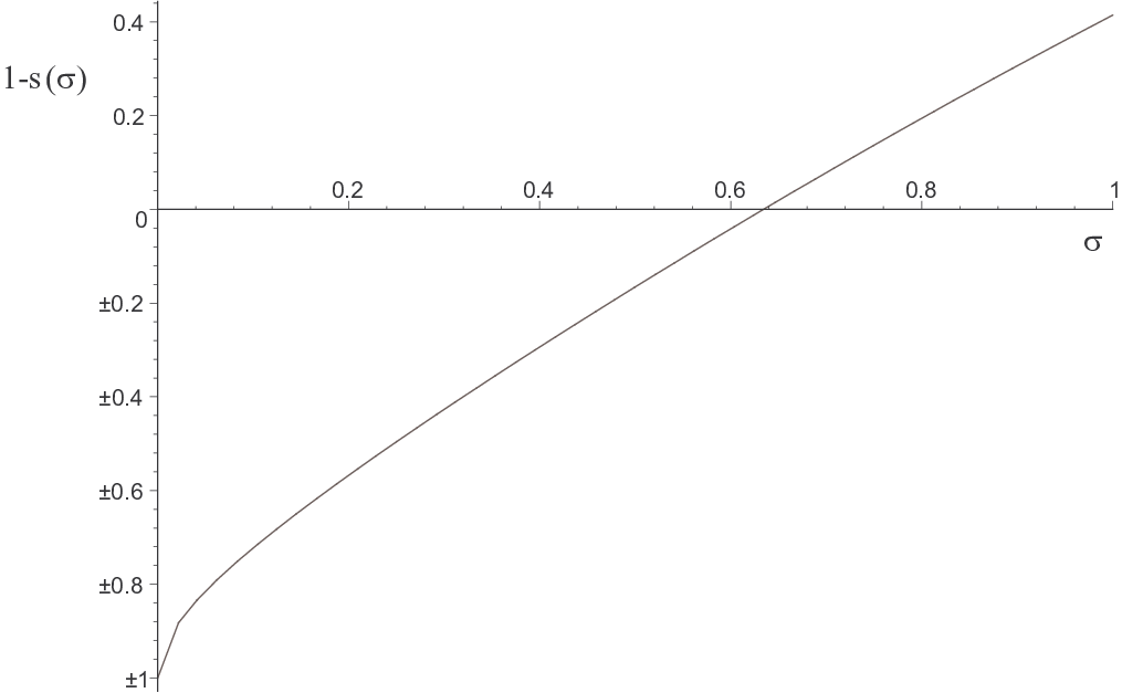
We can now characterize our lightlike shock-wave solution which we do in the following theorem.

Theorem 4.5.

Assume an equation of state of the form $\bar{p}=\bar{p}(\bar{\rho})$ for the TOV metric, and $p=\sigma\rho$ for the FRW metric. Also, assume that relation between $\sigma$ and $\bar{\sigma}$ , given by

\bar{\sigma}=\frac{1}{2}\sqrt{9\sigma^{2}-18\sigma+25}+\frac{3}{2}\sigma-\frac{5}{2}=H(\sigma)

holds, where we have taken $k=0$ . Then the TOV solution given by

\bar{\rho}=\gamma/\bar{r}^{2},

M(\bar{r})=4\pi\gamma\bar{r},

A=1-8\pi\mathcal{G}\gamma,

and

B=B_{0}\left(\frac{\bar{r}}{\bar{r}_{0}}\right)^{4\bar{\sigma}_{2}/(1+\bar{\sigma}_{2})}

will match the FRW solution given by

\rho(t)=\frac{3\gamma}{[\pm\sqrt{18\pi\mathcal{G}\gamma}(1+\sigma_{2})(t-t_{0})+\bar{r}_{0}]^{2}},

and

R(t)=R_{0}\left(\frac{\bar{r}(t)}{\bar{r}_{0}}\right)^{2/3(1+\sigma_{2})}

across the shock surface

\bar{r}(t)=\pm\sqrt{18\pi\mathcal{G}\gamma}(1+\sigma_{2})(t-t_{0})+\bar{r}_{0},

such that conservation of energy and momentum hold across the surface. We have used $\sigma_{2}$ , and $H(\sigma_{2})=\bar{\sigma}_{2}$ , where $\sigma_{2}$ is the solution of $s(\sigma)=1$ , and $s(\sigma)$ denotes the shock speed given in (4.92).

The Lax Shock Conditions

The final question we would like to answer is how do we classify the shock solution given in Theorem 4.5 with respect to the shock conditions first given by Smoller and Temple in [15]? As in [15] we only consider the case when the pressure and density are greater behind the shock wave. Since $\rho=3\bar{\rho}$ this means that the FRW region is behind the shock, the TOV region is in front of the shock. Therefore, for our solution we take the plus sign for expression of $\dot{R}$ in (4.9), and the corresponding signs in equations (4.10), (4.11), and (4.12).

The shock speed given in (4.92) is coordinate dependent, and is computed in a locally Minkowskian frame [4, 15, 16]. A coordinate system is called locally Minkowskian at a point $p$ if $g_{\alpha\beta}(p)=\mbox{diag}(-1,1,1,1)$ , but not necessarily Lorentzian where it is also required that $g_{\alpha\beta,\gamma}(p)=0.$ Also, note that since we are working with the radial component exclusively we only need to consider a locally Minkowskian frame in the $(t,r)$ -coordinates. We denote our locally Minkowskian coordinates by $(t,\tilde{r}),$ and they can be obtained by letting $r=\varphi(\tilde{r})$ and choosing $\varphi$ so that $\varphi^{\prime}=1/R^{2},$ which implies

ds^{2}=-dt^{2}+R^{2}dr^{2}\longrightarrow d\tilde{s}^{2}=-dt^{2}+d\tilde{r}^{2}.

The shock speed $s(\sigma)$ is determined in a locally Minkowskian frame comoving with the FRW metric.

Recall that we have chosen $\sigma=\sigma_{2}\approx 0.63442$ to satisfy $\dot{r}=1/R$ , and since

\dot{r}=\frac{dr}{dt}=\frac{1}{R}\frac{d\tilde{r}}{dt},

it follows that

s(\sigma_{2})=1,

in $(t,\tilde{r})$ -coordinates. The characteristic speeds behind the shock are equal to the sound speed $\pm\sqrt{\sigma}$ in the $(t,\tilde{r})$ -coordinate system, since the FRW fluid is comoving with respect to $(t,\tilde{r})$ -coordinates [15]. That is, the speeds of the characteristics relative to the FRW fluid are given by

\tilde{\lambda}^{\pm}_{FRW}\equiv\pm\frac{d\tilde{r}}{dt}=\pm\sqrt{\sigma}.

In our case, with the shock moving outward with respect to $r$ and $\bar{r}$ , the Lax characteristic condition, which says that the characteristic curves of the shock family impinge on the shock from both sides and all other characteristics cross the shock, hold if and only if

(4.95)

\tilde{\lambda}^{+}_{TOV}<s<\tilde{\lambda}^{+}_{FRW},

where $\tilde{\lambda}^{+}_{TOV}$ denotes the corresponding characteristic speed on the TOV side, or the front side, of the shock. Then in our lightlike case we have,

\tilde{\lambda}^{+}_{FRW}=\sqrt{\sigma_{2}}\approx\sqrt{0.63442}=.79650<1=s(\sigma_{2}),

which means that our shock solution does not satisfy the Lax characteristic condition. We can also conclude that

(4.96)

\tilde{\lambda}^{-}_{FRW}<\tilde{\lambda}^{+}_{FRW}<s(\sigma_{2}).

Now we would like to know how $s(\sigma_{2})$ relates to the characteristics $\tilde{\lambda}^{\pm}_{TOV}$ . In [15] Smoller and Temple show that

(4.97)

\tilde{\lambda}^{+}_{TOV}(\sigma)\equiv-\frac{2-\sqrt{\bar{\sigma}^{2}+6\bar{\sigma}+1}}{\sqrt{\bar{\sigma}^{2}+6\bar{\sigma}+1}-2\bar{\sigma}}\sqrt{\bar{\sigma}}.

Then for $\sigma=\sigma_{2}\approx 0.63442$ we have

\tilde{\lambda}^{+}_{TOV}(\sigma_{2})\approx-0.45040<1=s(\sigma_{2}),

see figure 4.3.

Therefore, we have that

\tilde{\lambda}^{-}_{FRW}<\tilde{\lambda}^{+}_{FRW}<s(\sigma_{2}),

and

\tilde{\lambda}^{-}_{TOV}<\tilde{\lambda}^{+}_{TOV}<s(\sigma_{2}).

Thus both sets of characteristics cross the shock since its speed is greater than the characteristic speeds on each side of the shock.

4.6. Comparison with the Smoller-Temple Sublight Shocks

In [15] Smoller and Temple show that in the limit as their subluminal shock solutions tend to the speed of light,

\sigma\longrightarrow\sigma_{2}=0.745

However, we have shown that an actual shock solution moving at the speed of light the value $\sigma_{2}=0.63442$ . This yields the unexpected result that the solution is not equal to the limit of Smoller-Temple subluminous solutions as they tend to the speed of light.

Chapter 5 Conclusions and Summary of Contributions

We have generalized the work of Smoller and Temple given in [14] and [15] in the sense that we can include lightlike shock surfaces. In defining a more general second fundamental form, by replacing the normal vector with a transverse vector satisfying the jump conditions (3.4) and (3.5), we were able to overcome the breakdown of the standard second fundamental form for lightlike hypersurfaces. Then we used this generalized second fundamental form, in an analogous way to how Smoller and Temple applied the standard second fundamental form in [14], to obtain a theory for the lightlike case. In the process, we introduced a modified Gaussian Skew coordinate system. This theory yielded the unexpected result of having to include the condition that the metric be $C^{2}$ on the spacelike subspace of $T_{p}\Sigma$ .

Then we were able to construct the an exact, spherically symmetric shock-wave solution of the Einstein equations which propagates at the speed of light. No quantities are moving at the speed of light except the shock. Although, our solution was consistent with Smoller and Temple’s results in [15], there was the unexpected difference in the value of $\sigma_{2}$ . In the non-lightlike computation given [15] the value for $\sigma$ in the lightlike limit was

\sigma_{2}\approx 0.745,

while our lightlike computations yielded

\sigma_{2}\approx 0.63442.

From this we conclude that the limit of the Smoller-Temple subluminal solution as it tends to the speed of light is not equal to our solution propagating at the speed of light.

Furthermore, we showed that in this exact solution the pressure and density are finite on each side of the shock throughout the solution, the sound speeds, on each side of the shock, are constant and subluminous. Moreover, the pressure and density are smaller at the leading edge of the shock which is consistent with the entropy conditions in classical gas dynamics [7, 13].

5.1. Summary of Contributions

In the lightlike shock matching theory of Chapter 3 we applied the notion of a generalized second fundamental form given by Barrabès and Israel in [1] into the shock matching framework of Smoller and Temple [14, 15]. The generalized second fundamental form $\mathcal{K}$ in [1] was given in a scalar form, and we modified it so that $\mathcal{K}$ is mapping that takes tangent vectors on the surface to tangent vectors on surface. Then we based the analysis on a Gaussian skew type coordinate system which we had to modify so that we could incorporate the generalized second fundamental form into the shock matching theory. Most of the supporting lemmas, and each of the theorems in [14] had to be modified and proved again in the context of this new Modified Gaussian Skew (MGS) coordinate system and the generalized second fundamental form. This yielded the unexpected result of adding the extra condition in our main result, Theorem 3.9, that the metric inner product on the spacelike subspace of $T_{p}\Sigma$ to be $C^{2}$ in order for the Rankine-Hugoniot jump conditions to hold. This condition was already satisfied for the spherically case in Theorem 3.24.

Then in Chapter 4 we constructed a new exact shock-wave solution moving at the speed of light. In order to do this we had to construct appropriate transverse vectors $N$ , and apply our extension of the subluminal theory to the specific example of the matched FRW/TOV metrics. This included significant modification of the equations expressing the Rankine-Hugoniot jump conditions given in equation (4.76). This yielded the difference in the limit of the Smoller-Temple subluminal solutions as they tended to the speed of light with the actual solution propagating at the speed of light. Lastly, we incorporated the modifications of the subluminal shock solutions to show that our new exact solution was a crossing shock.

General Relativistic Shock-Waves Propagating at the Speed of Light

Acknowledgements

Abstract

Notation and Conventions

Chapter 1 Introduction

1.1. The Central Problem: Lightlike Shock-Waves

The Two Difficulties of the Lightlike Case

1.2. How This Document is Organized

Chapter 2 General Relativity and the Second Fundamental Form

2.1. The Geometry of Spacetime

Special Relativity

Postulate 1 (Principle of Relativity).

Postulate 2 (Propagation of light).

Measuring Distance in a Special Relativistic Spacetime

Definition 2.1.

Summary 2.2 (Special Relativity).

General Relativity

The Metric in a Curved Spacetime

Tensors in Spacetime

Parallel Transport and the Derivative Operator

The Curvature Tensor

Proposition 2.3.

Einstein Tensor

2.2. Describing Matter in Spacetime

The Stress-Energy Tensor

Conservation of Energy and Momentum

2.3. The Einstein Equations

2.4. The Second Fundamental Form

The Induced Connection

Definition 2.4.

Definition 2.5.

Lemma 2.6.

Proof.

Chapter 3 Lightlike Shock-Wave Solutions of the Einstein Equations

3.1. Generalizing the Second Fundamental Form

The failure of the Second Fundamental Form in the Lightlike Case

Generalized Second Fundamental Form

Lemma 3.1.

Proof.

Modified Gaussian Skew (MGS) Coordinates

Lemma 3.2.

Lemma 3.3.

Proof.

Remark 3.4.

Lemma 3.5.

Proof.

Remark 3.6.

The Main Result of the Generalized Second Fundamental Form

Lemma 3.7.

Proof.

Corollary 3.8.

Proof.

3.2. The Main Theorem

Theorem 3.9.

3.3. Supporting Results

The Rankine-Hugoniot Jump conditions

Lemma 3.10.

Proof.

Lemma 3.11.

Proof.

Remark 3.12.

Lemma 3.13.

Proof.

Lemma 3.14.

Proof.

Lemma 3.15.

Proof.

Lemma 3.16.

Proof.

Theorem 3.17.

Proof.

Curvature Tensor Components as Delta Functions

Lemma 3.18.

Proof.

Corollary 3.19.

Proof.

Lemma 3.20.

Proof.

Theorem 3.21.

Proof.

General Relativistic Shock-Waves
Propagating at the Speed of Light

Relating to a $C^{1,1}$ metric by a $C^{1,1}$ transformation

Existence of Local Lorentzian Frame Via a $C^{1,1}$ Transformation

Bibliography

- [1] C. Barrabès and W. Israel, Thin shells in general relativity and cosmology: The Lightlike limit, Physical Review D 43 (1991), no. 4, 1129–1142.
- [2] Albert Einstein, The Meaning of Relativity, fifth ed., Princeton University Press, Princeton, New Jersey, 1922.
- [3] Lawrence C. Evans, Partial Differential Equations, Graduate Studies in Mathematics, vol. 19, American Mathematical Society, Providence, Rhode Island, 1998.
- [4] Jeff Groah, Joel Smoller, and Blake Temple, Solving the Einstein Equations by Lipschitz Continuous Metrics: Shock Waves in General Relativity, Handbuch der Physik, Germany, 2001, (to appear).
- [5] S.W. Hawking and G.F.R. Ellis, The Large Scale Structure of Space-Time, Cambridge University Press, New York, 1973.
- [6] W. Israel, Singular Hypersurfaces and Thin Shells in General Relativity, Nuovo Cimento B (11) 44 (1966), no. 1, 1–14.
- [7] Peter D. Lax, Hyperbolic systems of conservation laws and the mathematical theory of shock waves, Conference board of the mathematical sciences, Regional conference series in applied mathematics, vol. 11, Society for Industrial and Applied Mathematics, 1973.
- [8] John M. Lee, Riemannian Manifolds: An Introduction to Curvature, Graduate Texts in Mathematics, vol. 176, Springer-Verlag, New York, 1997.
- [9] Charles W. Misner, Kip S. Thorne, and John A. Wheeler, Gravitation, W. H. Freeman and Company, New York, 1973.
- [10] Barrett O’Neill, Semi-Riemannian Geometry with Applications to Relativity, Pure and Applied Mathematics, vol. 103, Academic Press, San Diego, 1983.
- [11] J. Robert Oppenheimer and Hartland Snyder, On Continued Gravitational Contraction, Physical Review 56 (1939), 455–459.
- [12] Bernard F. Schutz, A First Course in General Relativity, Cambridge University Press, Cambridge, 1985.
- [13] Joel Smoller, Shock Waves and Reaction-Diffusion Equations, second ed., Springer-Verlag, New York, 1983.
- [14] Joel Smoller and Blake Temple, Shock-wave solutions of the Einstein equations: The Oppenheimer-Snyder model of gravitational collapse extended to the case of non-zero pressure, Arch. Rational Mech. Anal. 128 (1994), 249–297.
- [15] by same author, Astophysical shock-wave solutions of the Einstein Equations, Physical Review D 51 (1995), 2733–2743.
- [16] by same author, Shock-Wave Solutions of the Einstein Equations: A General Theory with Examples, May 16-22 1999, Proceedings of the European Union Research Network’s Third Annual Summer School Training and Mobility of Researchers Program, Lambrecht (Pfalz) Germany, (to appear).
- [17] Blake Temple, Shock-Waves and Geometry, March 1998, Grant Proposal-NSF Applied Math, UC Davis Math 1998.
- [18] Robert M. Wald, General Relativity, University of Chicago Press, Chicago, 1984.
- [19] Frank W. Warner, Foundations of Differentiable Manifolds and Lie Groups, Graduate Texts in Mathematics, vol. 94, Springer-Verlag, New York, 1983.
- [20] Steven Weinberg, Gravitation and Cosmology: Principles and Applications of the General Theory of Relativity, John Wiley & Sons, Inc., New York, 1972.
Index
- Bianchi Identities §2.1
- coordinate transformation Theorem 3.23, Theorem 3.9
- causal structure §2.1
- Christoffel symbol §2.1, §2.1, §3.1
- comoving §2.1, §2.2
- connection §2.1, §2.4
- connection coefficients §2.1
- contact discontinuity §1.1
- cosmological principle §4.1
- covariant item 2
- covariant derivative §2.1
- delta function singularity §3.3, Corollary 3.19, Theorem 3.21, Theorem 3.9
- Einstein equations Chapter 2, §2.3, §2.4, §4.2
- Einstein summation convention §2.1, §2.1
- Einstein tensor §2.1, §2.3, §3.3
- energy §2.2
- Equivalence Principle §2.1, §2.1
- event §2.1
- first fundamental form §2.4
- four-momentum §2.2
- four-velocity §2.2
- General Covariance Principle §2.1
- geodesic §2.1
- geodesic equation §2.1
- homogeneous §4.1
- hypersurface §2.4, §2.4, §2.4, §3.1, Theorem 3.9
- isotropic §4.1
- jump conditions §3.3
- Rankine-Hugoniot Theorem 3.9, Theorem 3.9
- lightlike curve §2.2
- lightlike hypersurface Chapter 3, §3.1
- lightlike vector Definition 2.1
- local extension §2.4
- locally inertial §2.1, §2.1, §2.1
- locally Lorentzian §2.1, §2.1, Theorem 3.23, Theorem 3.9
- Lorentzian frame §2.2
- Lorentzian signature §2.1
- metric §2.1, Theorem 3.9
- Lipschitz continuous Theorem 3.9
- MGS coordinates §3.1
- Minkowski metric §2.1, §2.1
- Modified Gaussian Skew coordinates §3.1
- parallel transport §2.1
- perfect fluid §2.2
- Principle of Relativity Postulate 1
- Propagation of light Postulate 2
- proper time §2.2
- rest frame §2.2
- rest mass §2.2
- Ricci scalar §2.1, §3.3
- Ricci tensor §2.1, §3.3
- Riemann curvature tensor §2.1, §2.1, §3.3
- second fundamental form §2.4, §2.4
- definition Definition 2.5
- generalized Chapter 3, §3.1, §3.1, §3.1, §3.3, §3.3, Theorem 3.9
- tensor Definition 2.4
- shape operator Definition 2.5
- shock surface §3.1
- slice coordinates §2.4, §3.1
- spacelike curve §2.2
- spacelike vector Definition 2.1
- spacetime §2.1
- surface layer §1.1, §3.1, §3.3
- tensor §2.1
- curvature Corollary 3.19, Theorem 3.21, Theorem 3.9
- tensor transformation law §2.1
- timelike curve §2.2
- timelike vector Definition 2.1