Uniform Infinite Planar Triangulations
Abstract
The existence of the weak limit as of the uniform measure on rooted triangulations of the sphere with vertices is proved. Some properties of the limit are studied. In particular, the limit is a probability measure on random triangulations of the plane.
Subject classification: Primary 60C05; Secondary 05C30, 05C80, 81T40.
1 Introduction
1.1 Motivation
What is a generic planar geometry?
There are many different planar geometries. The most commonly used one is the Euclidean plane, but is it generic? Is it more natural than, say, the hyperbolic plane?
For simplicity, consider discrete planar geometries (realized as planar graphs). Now there are still many choices. The lattice is the graph most commonly associated with planar geometry, but there is no a priori reason to prefer it over the triangular lattice, or any other lattice. One possible approach is based on convenience, preferring at each time the most convenient framework to work with. Even by that criterion no single geometry is always the best. Thus, some recent results are naturally adapted to the triangular lattice [31].
When we use a lattice, we force much more structure into our geometry than the topological condition of planarity necessitates. Random planar graphs, such as Delaunay triangulations, have less enforced structure, but they still arise from the underlying Euclidean geometry. Is there a clear reason to prefer the Euclidean over the hyperbolic plane?
The approach used here is to consider a probability measure — in some sense a uniform measure — on planar geometries. Then we can ask what properties does a typical sample of that measure have. The way this is done is by considering discrete geometries, realized in the form of infinite planar triangulations, and finding an interesting distribution on them. Over finite planar triangulations the uniform measure is a natural choice. We prove the existence of a probability measure on infinite planar triangulations which is the limit of the uniform distributions on finite planar triangulations as their size tends to infinity. A sample of this measure is called the uniform infinite planar triangulation (UIPT). This model was suggested in [8], where Benjamini and Schramm show a.s. parabolicity of a wide class of distributions on infinite planar graphs under the condition of a uniform bound on the vertex degrees. Alas, the results there require the vertex degrees to be bounded, and hence do not apply to the UIPT.
The uniform finite planar triangulation and related objects have been studied by both combinatorists and physicists. Mathematical study is traced back to the 1960’s with Tutte’s attempts at the four color problem. In a series of papers Tutte was able to count the number of planar maps of a given size of various classes, including triangulations [32, 33, 34, 35]. One of the conjectures he raised is that almost all planar maps are asymmetric, i.e., have no non-trivial automorphisms.
Tutte later proved his conjecture for a specific class of planar maps [36]. Random planar maps (and triangulations among them) have been studied extensively since then by others, proving Tutte’s conjecture in a more general setting [29].
Previous research here focused on finite triangulations, but many of the results are about the asymptotic properties of planar maps and can be translated directly into claims about the infinite triangulations we study. Thus, there are results about the distribution of degrees in a uniformly chosen triangulation [18], the size of 3-connected components [7], and probabilistic 0-1 laws [6]. A key novel feature of this paper is that we consider instead a distribution on infinite maps. As it turns out, in some respects it is easier to work with the infinite object than it is with the finite maps.
Schaeffer found a bijection between certain types planar maps and labeled trees [30]. Chassaing and Schaeffer [12] recently used that bijection to show a connection between the asymptotic distribution of the radius of a random map and the integrated super-Brownian excursion. They deduce from this connection that the diameter of such a map of size scales as . While they work with planar quadrangulations and we with triangulations, it appears that such local differences are insignificant when large scale observations such as diameter, growth, separation, etc. are concerned. This phenomenon is referred to as universality.
The physicists study such triangulations under the titles of dynamic triangulations, closely related to 2-dimensional quantum gravity. There, the essential idea is to develop a quantum theory of gravity by extending to higher dimensions the concept of Feynman integrals on paths. Triangulations are used as a discretized version of a 2 dimensional manifold, and a function is averaged over all of them [3, 9]. Physicists are more interested in a continuous scaling limit of the discrete model, which is believed to exist.
Physicists introduced here the methods of random matrix models [14]. Through these methods and other heuristics many conjectures were made on the structure of such triangulations. In particular, it is believed that the Hausdorff dimension of the scaling limit of 2-dimensional quantum gravity is 4 [3]. For a good general exposition of quantum gravity see [2], as well as [1, 13].
Of particular interest is the KPZ relation [22] which relates critical exponents for a number of models on the plane and in 2 dimensional quantum gravity. This relation has been used to predict various exponents such as non intersection exponents for Brownian motion in the plane [16, 17]. Later a rigorous derivation of the same values was found using the process [24, 25, 26].
It is hoped that this work will be the foundation for a rigorous study into the scaling limit of random planar maps, and thereby enable a better understanding of the relation between random surfaces and critical models on smooth surfaces.
Section 2 summarizes some results on counting triangulations which are the basis for much of what follows. Section 3 describes some properties of the UIPT that follow directly from the formulas for counting triangulations. In particular, is shown that a.s. the UIPT has one end, i.e., the limiting process does not add any topological complications to the triangulation.
In Section 4 the existence of the limit distribution is proved. In Section 5 we gives another characterization of the UIPT by a locality property. This roughly means that different regions in the triangulation are independent of one another and that each region is uniformly distributed among all triangulations of a given size (and hence the name uniform triangulation for the infinite graph). Section 6 describes a multi-type Galton-Watson tree naturally associated with a UIPT.
In Section 7 we show a relation between two types of infinite planar triangulations that demonstrates the universality principle. Through this relation we also get an infinite form of the main result of [7] (see also [5]).
In a forthcoming paper (by the first author) [4], an alternative method of constructing and sampling the UIPT is given. Using this method, it is shown there that up to polylogarithmic factors the UIPT has growth rate , agreeing both with the heuristics for the Hausdorff dimension [3] and with the asymptotics for the radius of finite maps [12]. That paper also proves that the component of the boundary of the ball of radius separating it from infinity has size roughly . The method also enables an analysis of site percolation on the UIPT.
We proceed now to give formal definitions of the types of triangulations we study. An exact formulation of our main results will follow.
1.2 Definitions
The notion of a triangulation is very similar to the topological notion of a simplicial complex, although since we deal with the combinatorial aspects rather then the topological ones we will use a graph theoretic approach.
The notion of a triangulation has a bit of ambiguity around it. There are several variations on the definition, and they have much in common although there are some minor differences between them. The common thread to all variations is that a triangulation is a graph embedded in the sphere so that all faces are triangles. We will work with two types of triangulations.
Definition 1.1.
Consider a finite connected graph embedded in the sphere . A face is a connected component of . The face is a triangle if its boundary meets precisely three edges of the graph. Similarly, a face is an -gon if it meets edges. An embedded triangulation is such a graph together with a subset of the triangular faces of .
Let the support of be the union of and the triangles in . Two embedded triangulations are considered equivalent if there is a homeomorphism of and that corresponds and . is a triangulation of the sphere if . It is a triangulation of an -gon if is a single -gon.
For convenience, we usually abbreviate “equivalence class of embedded triangulations” to “triangulation”. This should not cause much confusion. The definition extends naturally to other manifolds, though we will not be concerned with that generality here.
Following the terminology found in [2] for types of triangulations, we define three classes of triangulations, types I, II and III. These differ according to which graphs are permitted in 1.1. In type I, there may be more than one edge connecting a pair of vertices, and loops (i.e., edges with both endpoints attached to the same vertex) are allowed as well. Type I triangulations will not be considered here, though some of the results (and proofs) apply to them as well.
Definition 1.2.
A type II triangulation is a triangulation where the underlying graph has no loops, but may have multiple edges.
Definition 1.3.
A type III triangulation is a triangulation where the underlying graph is a simple graph (having no multiple edges or loops).
Type II (resp. type III) triangulations are also referred to as 2-connected (resp. 3-connected) triangulations, since they are the triangulations with 2 or 3 connected underlying graphs.
If is a triangulation of a domain in the plane which may have several holes (i.e., several boundary components), we will refer to the holes of the domain as external or outer faces of . An external face may have 3 vertices on its boundary and then it is a triangle in itself. In that case that face is still distinguished from the triangles of . In the case of type II, an external face can also have only 2 vertices on its boundary.
It is worthwhile noting that the circle packing theorem [23] gives a canonical embedding in the sphere (up to Moebius transformations) of a type III triangulation of the sphere.
The vertices of lying on the boundary of its support are called boundary vertices, and those in the interior of are internal vertices. When we consider triangulations of a domain in the sphere with a number of boundary components we will usually fix the number of boundary vertices in each component as part of the domain. Thus, for example, a disc with boundary vertices will be distinguished from a disc with boundary vertices. Such a disc is referred to as an -gon.
The size of a triangulation , denoted , is defined as the number of internal vertices. Since all faces are triangles, by Euler’s characteristic formula, if (resp. ) is the number of edges (resp. faces) of , then (resp. ) is determined by the number and size of the boundary components of . In particular, for a sphere all vertices are internal, and so and .
Note that for a type III triangulation of the sphere (and even slightly more generally) the underlying graph determines the triangulation, i.e., whether any three edges form a triangle or not. When multiple edges are allowed there may be several distinct embeddings of the graph in the sphere giving distinct triangulations. E.g., in Figure 1.1 (c) and (d) are distinct triangulations that have the same underlying graph.

A fundamental problem encountered when studying planar maps (triangulations included) is that of symmetries, namely that some maps have non trivial automorphism groups. It seems plausible that most triangulations are asymmetric. While this has been proved [36, 29], we dispose of this problem in another manner. A simple way of eliminating any symmetries there are is by adding a root to the triangulation.
Definition 1.4.
A root in a triangulation consists of a triangle of called the root face, with an ordering of its vertices . The vertex is the root vertex and the directed edge is the root edge.
Note that in type II triangulations there may be more then one triangle with the same three vertices, so marking only the three vertices does not generally suffice. In a triangulation of the sphere, if the root edge is given, then there are exactly two possibilities for the root. We will usually mark only the root edge as in Figure 1.1, by an arrow.
When has a boundary we will usually assume that the root edge lies on the boundary. Since a disc with boundary vertices is referred to as an -gon, triangulations (a) and (b) of Figure 1.1 are of a square, while (c) and (d) are of a pentagon.
There are many possible variation on the definition of triangulation. Restricting to 2 or 3-connected underlying graphs (or even 4 or 5-connected) gives slightly different definitions. It is possible to restrict the degrees of vertices, or to allow faces that are not triangles. Thus quadrangulations as well as convex polytopes in general, can be described as a variation on the notion of triangulation. Most of the results proved below should have analogues for such generalizations, though the proofs do not always carry through and some complications are incurred in the transition. For convenience and brevity, we will deal with type II and type III triangulations here.
The definition of an embedded infinite triangulations is identical to that of finite triangulations, except that in that case is infinite, of course. However, we will generally require of our infinite triangulations to be locally finite, in the following sense.
Definition 1.5.
A triangulation embedded in the sphere is locally finite if every point in has a neighborhood in that intersects only a finite number of elements of (i.e., edges, vertices, triangles).
We will henceforth require all the triangulations under discussion to be locally finite. In particular this implies that the graph of is locally finite (each vertex is incident only to finitely many edges). However, this also requires that the embedding of is faithful to the combinatorial structure in the following sense: if is a sequence in belonging to distinct edges of , then accumulation points of must be outside of . The condition on the embedding is needed only so that the definition of equivalence of embeddings, as stated in the finite case, will also be useful in the infinite setting. It is possible to define triangulations from a completely combinatorial standpoint, and then embeddings may be ignored. However, the definitions are tricky, and it is convenient to think of triangulations as embedded in the plane or sphere.
A triangulation of the plane is a triangulation with for some . The sphere may be identified with the plane with mapped to a point at infinity. Thus this definition is equivalent to having with no accumulation points in .
A triangulation may be endowed with a metric in a number of ways. We will rather use a metric on the vertices of a triangulation — the graph metric induced by the underlying graph. It is also interesting to consider a triangulation as a metric space by having each face be isometric to an equilateral triangle with the shortest path metric on the whole triangulation. Then a triangulation of the sphere is a metric space homeomorphic to the sphere.
For either type, the space of finite and infinite (equivalence classes of) connected planar rooted triangulations is endowed with a natural topology described in [8]. (Note however, that there the root was only a vertex, leading to a closely related but slightly different notion). A sequence of rooted triangulations converges to a triangulation if eventually they are equivalent with on arbitrarily large combinatorial balls around the root. This is a metric topology: e.g., set , where is the maximal radius such that the combinatorial balls of radius around the roots are equivalent. In this topology, all finite triangulations are isolated points, and infinite triangulations are their accumulation points. It is not hard to check that is a metric; i.e., if , then is equivalent to (even when and are infinite).
Given a Cauchy sequence of locally finite embedded rooted triangulations it is easy to see that it is possible to choose for them embeddings that eventually agree on the ball of any fixed radius about the root. Thus, the limit of the sequence exists (as a locally finite embedded triangulation). In other words, the space of (locally finite embedded rooted) triangulations is complete.
This metric is non-Archimedean, i.e. which implies that if two balls in intersect, then one is a subset of the other.
Unlike in the setup of [8], the triangulation space is not compact. Consider the sequence of triangulations where contains two vertices of degree with the same neighbors forming a cycle (i.e., a double pyramid). Since are distinct and all have diameter 2, has no convergent subsequence.
We will be interested in the uniform distributions on triangulations:
Definition 1.6.
(resp. ) is the uniform distribution on rooted type II (resp. type III) triangulations of the sphere of size (i.e., having vertices).
The topology on the triangulation space induces a weak topology on the linear space of measures supported on planar triangulations. We study the distribution on infinite planar triangulations which is the weak limit of as :
Definition 1.7.
A measure on is the limit of if for every bounded continuous function
Since for any radius and triangulation the characteristic function of the event is continuous, implies convergence with respect to neighborhoods of the root; that is, for any and
| (1.1) |
However, since is not compact, the existence of for every and is not sufficient for convergence. Indeed, if are distributions on triangulations where the degree of the root vertex in is a.s. , then the probability of observing any given triangulation as the ball of radius tends to 0, but the weak limit does not exist in the sense of Definition 1.7. (It would not even be correct to say that , since .)
While the existence of the limits is not in itself sufficient for existence of a weak limit of , it follows from the equivalence of Definition 1.7 to convergence with respect to the Prohorov metric (see [15, §11.3]) that if is a probability measure satisfying (1.1) for every and , then . Indeed, for and let denote the set of all such that for some . Then is just the set of triangulations such that the ball in is the same as the ball in some . Given , we may find distinct such that . For all sufficiently large and for , we have . Given a Borel set , let be the set of such that . Then
holds for all sufficiently large and for all Borel sets . Consequently, in the Prohorov metric, and therefore also in the sense of Definition 1.7. Thus, understanding the limiting probabilities of balls is one of the key ingredients in proving that exists.
If and are rooted triangulations, we say that is contained in (and write ) if the two roots are the same and is contained in as unrooted triangulations. Sometimes we may also write to mean that there is a triangulation isomorphic to contained in .
Finally, a word on notation. By we mean that . By we mean that . We use to signify constants, whose actual value may change from one formula to another.
1.3 Main Results
We will first prove that
Theorem 1.8.
There exists a probability measure (resp. ) supported on infinite planar triangulations of type II (resp. type III) such that
Note. The proof of this theorem basically has two parts. The first is to show that for every and every finite triangulation , the limits exist. This part is based on the exact enumeration results, (and is not entirely new). Existence of these limits is a consequence of the well behaved asymptotic forms for the enumeration results, and can be extended to other classes of planar structures.
The second necessary ingredient is to prove tightness (Lemma 4.4), which is needed since the space is not compact. To see why tightness is necessary, the reader may wish to consider the sequence of probability measures on where . This sequence does not converge to any measure. However, for every . Similarly, it is easy to come up with examples of probability measures on where exists for every but the limit of does not exist.
Having established the existence of the limit measure (we will often drop the type notation when results hold for either type) we turn to study the a.s. properties of a sample of . Denote such a sample by UIPT. A basic geometric property, one endedness, will show that the limit structure maintains the plane’s topology. Recall the definition:
Definition 1.9.
A graph is said to have one end (is one-ended) if for any finite subgraph , contains exactly one infinite connected component.
Theorem 1.10.
The UIPT is a.s. one ended, and is therefore a triangulation of the plane.
We also ask about the electrical type of the underlying graph. In [8] it is shown that for any sequence of distributions on planar graphs with degrees uniformly bounded by , if a root is marked uniformly in each graph then every subsequential limit is a.s. recurrent. This holds, for example, for planar triangulations with uniformly bounded degrees. However, for those distributions it is not clear how to prove that the limit exists (simulations support this [10]). The following conjectures appear in [8]:
Conjecture 1.11.
For every , the distributions conditioned to have degrees uniformly bounded by are weakly convergent.
Conjecture 1.12.
The UIPT is a.s. recurrent.
VEL parabolicity (for vertex extremal length) is a property of infinite graphs, closely related to circle packings for planar graphs. In graphs with bounded degrees it is equivalent to recurrence [21]. The proof in [8] of a.s. VEL parabolicity for uniform infinite triangulations with bounded degrees is still valid for the UIPT, with tightness (Lemma 4.4) filling the role of bounded degrees.
Acknowledgments: We thank Itai Benjamini and Bálint Virág for inspiring conversations. Part of this research was done during visits of the first author to Microsoft Research. The first author thanks his hosts for these visits.
2 Counting
2.1 Classical Results
Much of the analysis of triangulations is based on counting them. This is true both for finite triangulations and for infinite triangulations where the asymptotics of the finite triangulations come into play. The following counting results go back to Tutte [32] who counted various types of planar maps and triangulations. The results we use here are not due to Tutte but are derived using the same technique he uses. More details can be found in [11]. A good account of the technique including all results given here can be found in [20].
Theorem 2.1.
- 1.
For , not both 0, the number of type II triangulations of a disc with boundary vertices and internal vertices that are rooted on a boundary edge is
- 2.
For , the number of rooted type III triangulations of a disc with boundary vertices and internal vertices that are rooted on a boundary edge is
The case for type II triangulations warrants special attention. A triangulation of a 2-gon must have at least one internal vertex so there are no triangulations with , yet the above formula gives . It will be convenient to use this value rather then 0 for the following reason. Typically, a triangulation of an -gon is used not in itself but is used to close an external face of size of some other triangulation by “gluing” the boundaries together. When the external face is a 2-gon, there is a further possibility of closing the hole by gluing the two edges to each other with no additional vertices. Setting takes this possibility into account.
Since we will consider the asymptotics of large triangulations we will need the following estimates of these numbers. Using the Stirling formula, as we have the following:
where and
For type III triangulations we have similar estimates:
where and as :
Much of the time we will not distinguish between type II and type III triangulations. The type index will be dropped either when the stated results hold for both types or when it is be clear which type is discussed.
We are interested in triangulations of the sphere that have no predefined boundary. The number of those is given by:
Proposition 2.2.
For either type, the number of rooted triangulations of the sphere with vertices is .
Proof.
Adding a triangle that closes the outer face of a triangulation of a triangle makes a triangulation of the sphere. Alternatively, removing the triangle incident on the root edge that is not the root triangle gives a triangulation of a triangle rooted on the boundary. Thus, there is a bijection between triangulations of the sphere with vertices and triangulations of a triangle with internal vertices. ∎
We will also be interested in triangulations of discs where the number of internal vertices is not prescribed. The following measure is of particular interest:
Definition 2.3.
The free distribution on rooted triangulations of an -gon, denoted , is the probability measure that assigns weight
to each rooted triangulation of the -gon having internal vertices, where
As before, (resp. ) will denote free type II (resp. type III) triangulations, and similarly for the partition functions and . Thus, the probability of a triangulation , is proportional to , and acts as a normalizing factor.
Note that by the asymptotics of as we see that the sum defining converges for any and for no larger . The value of the partition functions will be useful. For this we have:
Proposition 2.4.
- 1.
For type II triangulations, if :
- 2.
For type III triangulations, if :
At the critical point we will omit . There takes the values:
and
The proof can be found as intermediate steps in the derivation of in [20]. The above form may be deduced after a suitable reparametrization of the form given there.
2.2 Universality
While the exponential term in the asymptotics of is different for type II and III, the next term of is the same. Similarities also occur in the asymptotics of and of for the two types. Those similarities are not coincidental. It turns out that the asymptotic form is quite common when counting 2 dimensional structures. That form of the asymptotics is not dependent on the manifold, and is valid for any 2-dimensional manifold with or without boundaries. The same forms also appear when instead of triangulations other types of maps are considered, and was found to hold for a large variety of map types ([10, 9] and also the result of [12], related to our growth results). We therefore believe that many of the results on the UIPT hold in a much more general context. In this, infinite planar objects are similar to random walks, critical percolation and many other critical models where the large scale properties are independent of the local lattice.
This universality is related to the basic property of the -sphere that a cycle partitions it into two parts, i.e., the Jordan Curve Theorem. This leads to a similarity between recurrence relations for different types of structures and through them to similar asymptotics for the solutions. For another instance of universality and some explanation see [5].
It turns out that the exponential part of the asymptotics will cancel out often and when finer properties of infinite triangulations are considered the power term will come into play and determine the observed behavior.
2.3 Some Estimates
We will need the following estimates throughout the paper.
Lemma 2.5.
Let
then for any there is a such that for any :
Proof.
Clearly
since each term in the sum over ordered -tuples corresponds to at most terms in the original sum, and less if there are any repetitions. Since each possible choice of determines a unique value for and always we can replace by the smaller and extend the range of summation.
∎
3 Basic Properties
3.1 Invariance with respect to the Random Walk
If we are given a finite triangulation, but not the location of the root, what can we say about the location of the root? The following proposition says that not much. For a triangulation and a possible root in let denote the triangulation with marked as root (if is rooted then the old root is no longer marked).
Proposition 3.1.
Let be a sphere triangulation chosen by , and be a root in chosen uniformly among all possible roots. Then is uniformly distributed among all rooted triangulations (of size ).
Proof.
At first glance this seems trivial: since all rooted triangulations are equally likely no triangle in should be more likely to be the root than any other. However, there is a subtlety here since there may be several triangles such that the triangulations are isomorphic. This occurs whenever has a non trivial automorphism.
The key fact here is that any automorphism of that preserves a root is necessarily the identity automorphism. If is the set of possible roots and is the automorphism group of as an unrooted triangulation, then acts naturally on and a non identity element of has no fixed points in . Thus, the size of the orbit of a triangle is just the size of , regardless of .
Since each of the orbits in the action of on corresponds to a distinct rooted triangulation, and each orbit has the same size, each possible triangulation is equally likely to result after a new root is selected. ∎
Note that since each directed edge can be completed in two ways to a root each directed edge is equally likely to be the root edge. From this we see that the UIPT must be invariant with respect to a random walk:
Theorem 3.2.
Let be a triangulation chosen by for some or by a subsequential limit . If is the root vertex of , is a uniformly chosen neighbor of , and is a triangle in uniformly chosen among all triangles including , then has the same law as .
Proof.
For finite , if a vertex of degree is the root vertex, then there are possibilities for the root edge (and options for the root). It follows that the probability that is the root is proportional to its degree. This is the stable distribution for the random walk on the graph of , so as a consequence of Proposition 3.1 we see that has the same law as .
Since this is true for every , the same holds for any subsequential limit. ∎
3.2 One Endedness
We start with a lemma describing the behavior of a triangulation on a disjoint union of discs.
Lemma 3.3.
Given disjoint polygons (with given boundary sizes) and a triangulation of the polygons, let be the number of internal vertices in the ’th polygon. Then
where depends only on the number and sizes of the boundaries of the polygons.
Proof.
We prove that the number of triangulations where is small, as required. By symmetry, the number for any other pair has the same bound. Since the number of such pairs, , does not depend on or on , this suffices.
We use the upper bound ( is only necessary to account for , and is not essential). Assume the ’th domain has boundary size . The number of triangulations we wish to bound is:
where at the end we used Lemma 2.5. ∎
Generally a limit of a sequence of finite sphere triangulations need not have support which is homeomorphic to the sphere or even the plane. While the limit is still planar, when embedded in the sphere may have any number of accumulation points. One accumulation point gives a punctured sphere, i.e., the plane. More than one means that has a more complicated topological structure; it is no longer simply-connected.
Corollary 3.4.
Every subsequential limit of a.s. has one end.
Proof.
Suppose that a subsequential limit has more then one end with positive probability. Then for some and some the probability that a loop of length including the root partitions a sample of into two infinite parts is at least . This implies that for any for infinitely many the -probability of having a loop of length including the root that has at least vertices on either side is at least . Call such a loop a separating loop.
Count pairs with a triangulation of size and a separating loop included in . From Lemma 3.3 we know that the total number of such pairs is . However, the total number of sphere triangulations with vertices is , and by dividing we deduce that the expected number of separating loops is . In particular as so does the probability that a separating loop exists. ∎
4 Existence of the Limit
4.1 Tightness
Given the formula for the number of disc triangulations (or even its asymptotics), it is simple to verify that the probability of observing any given ball around the root converges to some limit. However, since is not compact this is not sufficient to guarantee convergence of the measures. The missing factor is a tightness result for the measures.
Recall that a family of random variables is tight with respect to if
uniformly with respect to . More generally, a family of probability measures on a topological space is tight if for any there is a compact set with for all .
We first need to prove that the uniform measures on finite triangulations are a tight family. To this end, we first prove the following estimates for the degree of the root in either type of triangulation. While the lemmas are very similar in nature, the methods of proof given here are different. This demonstrates the underlying unity of the different models, while local differences make some techniques applicable in one and others in another. The following two Lemmas appear in similar form in [18].
Lemma 4.1.
Denote the degree of the root vertex by . For any there is a such that
uniformly for all and
Proof.
A type III triangulation of the sphere where the root vertex has degree is the union of two triangulations, whose intersection is a -gon: contains the root vertex and triangles connecting it to the sides of the -gon, and contains all other triangles. The root triangle has one edge in the intersection of and . Choose this edge to be the root edge of . Now is a bijection between rooted triangulations of the sphere with and rooted triangulations of a -gon with the root edge on the boundary.
If , then , and we know the number of such triangulations. Dividing by the number sphere triangulations, we get:
To prove the uniform exponential bound consider the ratio
for any sufficiently large . ∎
For type II, since multiple edges are present, there are two notions of degree. The vertex degree of is the number of neighbors it has, while the edge degree of is the number of edges incident on it. For our purposes bounding the vertex degree is sufficient, but in what follows we bound the larger edge degree.
Lemma 4.2.
Denote the edge degree of the root vertex by , then for any there is a such that
uniformly for all .
Proof.
Let be the triangles incident with the root vertex, ordered counterclockwise starting with the root triangle . For let be the sub-triangulation including triangles . Adding one at a time, we consider the distribution of conditioned on , and show that for any there is a probability bounded away from 0 that .
may have several external faces. One of those, say , includes the root vertex, and is in . In order for to be the last triangle adjacent to the root vertex it must include the two edges of on either side of the root vertex. Thus, in Figure 4.1(a), the triangles incident with the root vertex are numbered. The triangle is the final triangle, and it includes both the edge from and the edge from the root triangle . Note that when triangle is added, an unknown part of the triangulation is enclosed, but this will not effect the bounds we get.

To bound from below the probability that is the last triangle conditioned on , assume that the boundary of has size . At first condition on the event that the part of the triangulation inside has vertices. The number of possible ways to triangulate under these constraints is . If is the last triangle around the root, then adding it leaves a face of boundary size with internal vertices. Thus the probability of the next triangle being the last one is:
If , then this is at least 2/27, so the probability that is at most 25/27. Since this bound is uniform it also holds when conditioning only on and not on the number of internal vertices in .
Thus, as new triangles are revealed, each triangle has a probability of at least 25/27 of being the last one, unless . If , as for in Figure 4.1(b), then after a triangle is added we must have and so out of every two consecutive , at least one has . It follows that the probability of having more than edges leaving the root vertex is at most , as claimed. ∎
Note. For type III triangulations, Lemma 4.1 gives the exact probability of any given degree in the UIPT. To a large extent, this is possible because the radius 1 neighborhood of the root has a simple structure. When multiple edges are allowed, even the ball of radius 1 around the root can have a complicated structure, making an exact calculation harder to get. On the other hand, for type II triangulations, we can calculate the exact probability that a certain triangle is present in the triangulation conditioned on some sub-triangulation (e.g., the probability that is the last triangle around the root conditioned on , as in the proof). This is much harder to do for type III triangulations, because we need to keep track of which pairs of vertices already have edges between them, whereas in type II triangulations adding another edge is always legal.
At this point we will rigorously define the ball of radius around the root (or any other vertex, for that matter). This ball is a sub-triangulation, but there is some subtlety in its definition. The vertices of are all those vertices at distance at most from the root vertex, but not all edges and triangles between these vertices are necessarily part of .
Definition 4.3.
is just the root vertex itself. is composed of all triangles incident on any vertex of together with their vertices and edges.
Note that there may be edges between vertices on the boundary of that are not part of itself. Next, we turn our attention to the size of the ball . The following lemma holds for both types.
Lemma 4.4.
For any fixed the random variables (i.e., the maximal degree in ) defined on with measure are tight with respect to .
Proof.
For , is just the root, and Lemmas 4.1 and 4.2 show that the degree of the root is tight with respect to for either type.
We proceed by induction on . Suppose that is tight with respect to . To show that is also tight we use Theorem 3.2. Let denote a sample of , and let be a simple random walk on started at the root vertex . Denote by the resulting probability measure on triangulations with paths beginning at the root. It follows from Theorem 3.2 that for any the degree of has the same distribution as the degree of the root. Fixing we estimate the probability that and yet . Conditioned on this event, there is at east one vertex with . Since there is a path of length from the root vertex to , and all vertices on the path have degrees at most ,
and so
By Theorem 3.2 the LHS does not depend on and is simply . The RHS does not depend on the random walk either, so for any
By induction, for all we may choose such that for all . Then we take sufficiently large so that for all . This gives for all , and completes the proof. ∎
Corollary 4.5.
The family of probability measures is tight.
Proof.
Since for any there are only finitely many radius balls with , if is any sequence, then the set of triangulations with is compact. From tightness of it follows that for any there is a sequence so that for all . ∎
Since any tight family of probability measures on a complete separable space has a converging subsequence (see [15, Theorem 11.5.4]), this implies
Corollary 4.6.
Every subsequence of has a subsubsequence converging to a probability measure.
4.2 Taking the Limit
In [28] it is shown that for every finite triangulation there is a constant such that asymptotically, in almost every sphere triangulation of size the number of times appears is roughly . This is roughly the probability that a neighborhood of the root in the UIPT is isomorphic to . In fact, the result of [28] is stronger, since it gives not just an annealed probability of seeing but that the quenched probability is constant. We bring here a simpler calculation just for the annealed probability, since the results of the calculation are useful in what follows.
It will be easier to work with rooted triangulations having the property that if they are a sub-triangulation of the UIPT, then they appear in it exactly once. This is not only the case: a root triangle together with a cycle of some length may appear in the triangulation in several different ways.
Definition 4.7.
A rooted triangulation is rigid if it is connected and no triangulation includes two distinct copies of with coinciding roots.
The balls of a triangulation are rigid, as is evident from the following sufficient criterion for rigidity (the proof is left to the reader).
Lemma 4.8.
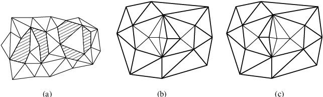
If in the dual graph of triangulation the vertices corresponding to the triangles form a connected set, and every vertex of is incident on a triangle, then is rigid.
This criterion is not necessary for rigidity, as is demonstrated by Figure 4.2(a), where there is an isolated triangle. In fact a sufficient and necessary criterion is that the support be 3-connected. In order to complete a planar triangulation to a sphere triangulation we need to fill each of its external faces with some triangulation. The advantage of rigid triangulations is that filling the external faces in different ways must lead to distinct sphere triangulations, whereas for non-rigid triangulations different ways of filling the faces may give rise to the same complete triangulation. Figure 4.2(b,c) give an example of a non-rigid triangulation and how two completions give rise to the same triangulation.
A second consequence of the construction of , whose proof (an application of the Jordan curve theorem) is left to the reader is:
Lemma 4.9.
In the ball there are no edges between two vertices of any external face except those making the face itself.
Proposition 4.10.
Let be a rigid rooted triangulation having no edges between two vertices of an external face except those making the face itself. Assume has vertices, some of which are on external boundary components of sizes . Then every subsequential limit of has:
Moreover, the probability that the ’th face is the infinite one corresponds to the ’th term in the sum, i.e.:
Note. For type II triangulations the restriction on edges between vertices of an external face is not necessary. For type III triangulations it is needed, since when such an edge exists it imposes restrictions on the component inside the face. In general, the probability that can be found using the proposition together with the inclusion-exclusion principle. The requested probability is a linear combination of a fixed number of terms and each of them has a limit as above.
Proof.
Let be a subsequential limit of . Denote by the event that (with the A’s root corresponding to ’s root) and that the part of in the ’th external face of contains internal vertices. This is defined in the finite as well is the infinite setting (though we keep ). In what follows denotes the number of vertices in the 1st external face, i.e., . The probability of is:
and is the sum over all possible vectors of this probability.
We first consider the limit:
Since the limit exists, it equals . This may be written as:
| (4.1) |
Of course, a similar expression holds when the role of the 1st face is filled by some other face, i.e., the sizes of all but the ’th face are fixed.
Proof of Theorem 1.8.
Corollary 4.6 tells us that a subsequential limit exists. It remains to prove that the limit does not depend on the subsequence. Since the balls are rigid, Proposition 4.10 shows that for every , does not depend on the subsequence. Since the sets form a basis for the topology on , this implies that does not depend on the subsequence. ∎
5 Locality
Next, we look at another basic property of the UIPT, namely locality. The meaning of locality is that isolated regions of the UIPT are almost independent. In the following, will denote the event defined in the proof of Proposition 4.10.
Theorem 5.1.
Let be a finite rigid triangulation (for type III, with no edges between vertices on external faces). Assume has external faces of sizes . Condition on the event , and let denote the component of the UIPT in the ’th face. Then:
- 1.
The triangulations are independent.
- 2.
has the same law as the UIPT of an -gon (that is, the limit of the uniform measure on rooted triangulations of an -gon with internal vertices).
- 3.
For , has the same law as the free triangulation of an -gon.
Proof.
Thus, we see that conditioned on the sizes of the ’s are independent, and is distributed like the free triangulation of an -gon. Consider . Conditioned on , since all possible triangulations of the sphere with the prescribed component sizes are equiprobable, the same holds for each component . Thus, for any the joint distribution of conditioned on their sizes is a product distribution. As , these joint distributions converge to the product distribution, where is uniform on triangulations with .
Finally, the marginal of has size tending to infinity, and so converges to the UIPT of an -gon. ∎
6 Ball Structure
Recall that Theorem 5.1 tells us that conditioned on a sub-triangulation , with some external faces, the probability that a face of size is the infinite one is proportional to . In the case of type II or III triangulations we have:
so in either case the probability of a face of size being the infinite face is roughly proportional to .
We wish to study the relation between the ball of radius and the ball of radius . The ball of radius is a finite triangulation with any number of external faces with any combination of boundary sizes. Moving to we add in each outer face some triangles around its circumference. These added triangles can fill up the face, or they can split that face up into a number of sub-faces of different sizes. Figure 6.1(a) shows a ball with several finite faces, and the layer of the triangulation between radius and in the finite faces. The shaded areas are some of the faces of the ball of radius . The infinite face may contain additional sub-faces.
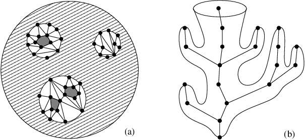
This gives rise to a tree-like structure for the triangulation, as in Figure 6.1(b). Each outer face of the ball of radius corresponds to a vertex in the ’th level of the tree. The face corresponding to a child is contained in the face of the parent vertex. An infinite triangulation will yield an infinite tree. Similarly, if a triangulation is one ended, then so is the corresponding tree, i.e., the tree is composed of a single infinite branch from the root with finite sub-trees growing from it. Note that while any triangulation determines a tree, the converse is false. The tree does not determine the triangulation.
A vertex in the tree corresponds to an external face of some triangulation, so there are different types of vertices depending on the face sizes. Labeling each vertex with the boundary size of the corresponding face, we see that the UIPT gives rise to a multi-type tree process.
From Theorem 5.1 we see that if we condition the first levels of the tree and on which vertex in the ’th level is in the infinite branch, then Theorem 5.1 tells us that the remaining sub-trees are independent. Thus, we see that at each level, one vertex, with a known distribution, has an infinite sub-tree above it, and the others have independent numbers of offspring of independent types. The tree process is thus just a multi-type Galton Watson process conditioned to survive. Without the conditioning we get the tree corresponding to a free triangulation of the sphere, which we know to be a.s. finite. However, since the free process has a power tail on its size, it is critical. Thus, the above description is just the construction of a critical Galton Watson process conditioned on survival (see [27]).
7 Type Relations
The two types of UIPT are part of a wider class of random planar object satisfying common properties. This was first hinted at by the universality of the asymptotic formulas for counting various planar objects. Between type II and type III triangulations there is a more fundamental relation, enabling us to find a direct transformation between type II and type III triangulations. A similar transformation also holds between type I and type II triangulations as well as other pairs of classes of planar objects.
Roughly, the idea for passing from a type II triangulation to a type III triangulation is to take each double edge and to remove all the triangles and vertices inside it. The two edges are then glued together to get again a triangulation of the plane or sphere as the case may be. Conversely, to get from a type III triangulation to a type II one, we will take each edge and replace it with a double (or multiple) edge with some distribution on the triangulation inside the resulting 2-gons. Recall that we allowed the triangulation of the 2-gon with no internal vertices, and gluing it in a 2-gonal outer face meant gluing the two edges together. Thus, with some probability ( actually) this empty triangulation is used and the edge remains a single edge.
Both directions pose some difficulties. A 2-gon partitions a triangulation to two components. How do we decide which is the inside and which the outside? In an infinite triangulation of the plane we wish to contract the finite side, but for a finite triangulation of the sphere it is not so clear. Also, there is the possibility that the root of the triangulation is deleted in this way, and then a new root is needed.
In the opposite direction, there is the question of the distribution for the triangulation of the 2-gon added. The natural candidate in the infinite case is the free triangulation of the 2-gon. Again, in the finite setting things are more delicate. Since we define the infinite triangulation measures as limits of the finite ones, we need to find some transformation of the finite measures first.
For a type II triangulation , when we contract 2-gons as described above, until no double edges remain, the result is a maximal (with respect to inclusion) 3-connected sub-triangulation, since the only way 2 vertices could separate the graph is by forming a 2-gon. Therefore, the transition can be summarized as taking a single maximal 3-connected subgraph of the triangulation. The natural choice for this is to take the 3-connected component containing the root triangle. This also saves us the trouble of choosing a new root in the case that the old root was in one of the contracted 2-gons. Note that the root vertex or even the root edge is not enough, since 2 vertices may be in the intersection of two distinct 3-connected components. However the 3 vertices of any triangle determine a unique 3-connected component.
Definition 7.1.
Let be a rooted type II triangulation. Define to be the type III triangulation composed of the 3-connected component of the root in , with all double edges identified into single edges. For a measure on rooted type II triangulations let be the resulting measure on type III triangulations, i.e., for any event :
This operation is known as taking the core of a structure [5]. In general, for two classes of rooted planar objects, one more restricted than the other, the core of a member of the wider class is its largest partial structure containing the root included in the smaller class (when it is unique).
Lemma 7.2.
For any finite , for some coefficients :
In the limit, for some constants :
In the infinite case this means that the 3-connected component of the root is either a finite sphere triangulation with some distribution on the size where all triangulations of the same size are equiprobable, or it is an infinite triangulation. Conditioned on the latter case it is just the infinite type III UIPT. The asymptotics of the coefficients are described in [5]
Proof.
Consider first the finite case. All we need to show is that any two type III triangulations have the same probability of appearing as the 3-connected component of the root in , i.e., that for any triangulation the number of triangulations with and depends only on .
This is clear, since any two triangulations of the same size have the same number of edges. Specifically, has edges. Formally, if is the generating function for triangulations of a 2-gon, then the number of ways can come about is the coefficient of in , which is, of course, determined by .
The infinite case follows from the finite case by taking a weak limit. The map is continuous with respect to the topology on the spaces of type II and III triangulations. Since is supported on triangulations with vertices, they have disjoint supports for distinct . Therefore, necessarily:
where must exist and
is the part of the measure that tends to infinity. In the infinite case, we can also give an explicit formula for . This is done in much the same way that we calculated the probability of a given ball when proving the limit of exists. Indeed, to find the probability for some type III triangulation with we just need to find the probability when each edge is replaced by an external face of size 2. By Proposition 4.10 this is:
(A sphere triangulation with vertices has edges). Substituting and the values of this translates to:
Since there are possible triangulations of size , the probability is:
In order to find we need to sum . Since is a linear combination of and , the generating function is a linear combination of and its derivative. Using that we find: and the remainder:
∎
Since we know that the UIPT is a.s. one ended, it has at most one infinite 3-connected component. The above calculations tell us more. We see that with probability 1/2 the root triangle is part of the infinite 3-connected component. In fact, if the root is in a finite 3-connected component, then this component has a number of 2-gonal external faces, and the infinite one contains a triangulation with the same LAW as the original UIPT. Iterating this we see that there is always a unique infinite 3-connected component, and with probability 1/2 the root is part of it. This is an infinite version of an asymptotic result on finite triangulations found in [19]. In fact, we know now the distribution of the size of the 3-connected component of the root, as is the asymptotic probability that the component has size .
How do we get back from the type III UIPT to the type II UIPT? We need to find the distribution of a UIPT conditioned on including an infinite triangulation. Theorem 5.1 deals with the UIPT conditioned on containing a finite sub-triangulation, and by conditioning on a growing subsequence of triangulations, we see that to get back from the infinite 3-connected component to the whole type II triangulation we need to replace each edge of with a free triangulation of a 2-gon.
Note that the expected number of triangles in a free triangulations of a 2-gon is twice the expected number of internal vertices and so is 2/3 (again, this is the derivative of at ). Since a triangulation contains 3/2 times as many edges as triangles, we see that in some sense in the resulting type II triangulation 1/2 the triangles were in the original type III triangulation and 1/2 were added.
As a consequence of this relation, some results on the type II UIPT are valid for type III as well. Those include the results on growth and on percolation derived in [4], among others.
References
- [1] J. Ambjørn. Quantization of Geometry. Lectures presented at the 1994 Les Houches Summer School “Fluctuating Geometries in Statistical Mechanics and Field Theory”. arXiv:hep-th/9411179.
- [2] J. Ambjørn, B. Durhuus and T. Jonsson. Quantum Gravity, a Statitstical Field Theory Approach. Cambridge Monographs on Mathematical Physics, 1997.
- [3] J. Ambjørn and Y. Watabiki. Scaling in quantum gravity. Nucl. Phys. B 445 (1995), no. 1, 129–142.
- [4] O. Angel. Growth and Percolation on the Uniform Infinite Planar Triangulation. submitted, arXiv:math.PR/0208123.
- [5] C. Banderier, P. Flajolet, G. Schaeffer and M. Soria. Random maps, coalescing saddles, singularity analysis, and Airy phenomena. Analysis of algorithms (Krynica Morska, 2000). Rand. Struc. Alg. 19 (2001), no. 3-4, 194–246.
- [6] E. A. Bender, K. J. Compton and B. L. Richmond 0-1 laws for maps. Random Struc. Alg. 14 (1999), no. 3, 215–237.
- [7] E. A. Bender, B. L. Richmond and N. C. Wormald. Largest 4-connected components of 3-connected planar triangulations. Random Struc. Alg. 7 (1995), no. 4, 273–285.
- [8] I. Benjamini and O. Schramm. Recurrence of Distributional Limits of Finite Planar Graphs. Elec. J. Prob., 6 (2001), paper no. 23.
- [9] D. V. Boulatov and V. A. Kazakov. The Ising Model on a Random Planar Lattice: the Structure of the Phase Transition and the Exact Critical Exponents. Phys. Lett. B 186 (1987), no. 3-4, 379–384.
- [10] M. J. Bowick, S. M. Catterall and G. Thorleifsson. Minimal Dynamical Triangulations of Random Surfaces. Phys. Lett. B 391 (1997), no. 3-4, 305–309.
- [11] W. G. Brown. Enumeration of triangulations of the disk. Proc. London Math. Soc. (3) 14 (1964) 746–768.
- [12] P. Chassaing and G. Schaeffer. Random Planar Lattices and Integrated Super-Brownian Excursion. arXiv:math.CO/0205226.
- [13] F. David. Simplicial Quantum Gravity and Random Lattices. Gravitation et quantifications (Les Houches, 1992), 679–749, North-Holland, Amsterdam, 1995. arXiv:hep-th/9303127.
- [14] P. Di Francesco, P. Ginsparg and J. Zinn-Justin. 2D Gravity and Random Matrices. Phys. Rep. 254 (1995), no. 1-2.
- [15] R. M. Dudley. Real analysis and probability. Wadsworth & Brooks/Cole Advanced Books & Software, Pacific Grove, CA, 1989.
- [16] B. Duplantier. Random walks, polymers, percolation, and quantum gravity in two dimensions. STATPHYS 20 (Paris, 1998). Phys. A 263 (1999), no. 1-4, 452–465.
- [17] B. Duplantier. Random walks and quantum gravity in two dimensions. Phys. Rev. Lett. 81 (1998), no. 25, 5489–5492.
- [18] Z. Gao and B. L. Richmond. Root vertex valency distributions of rooted maps and rooted triangulations. Europ. J. Comb. 15 (1994), no. 5, 483–490.
- [19] Z. Gao and N.C. Wormald. The size of the largest component in random planar maps. Siam J. Disc. Math. 12 (1999) no. 2, 217-228.
- [20] I.P. Goulden and D.M. Jackson. Combinatorial enumeration. New York, Wiley, 1983.
- [21] Z. X. He and O. Schramm. Hyperbolic and parabolic packings. Disc. Comp. Geom. 14 (1995), no. 2, 123–149.
- [22] V. G. Knizhnik, A. M. Polyakov and A. B. Zamolodchikov. Fractal structure of 2D-quantum gravity. Mod. Phys. Lett. A 3 (1988), no. 8, 819–826.
- [23] P. Koebe. Kontaktprobleme der konformen abbildung, Berichte Verhande. Sächs. Akad. Wiss. Leipzig, Math.-Phys. Klasse 88 (1936) 141–164.
- [24] G. Lawler, O. Schramm and W. Werner. Values of Brownian intersection exponents. I. Half-plane exponents. Acta Math. 187 (2001), no. 2, 237–273.
- [25] G. Lawler, O. Schramm and W. Werner. Values of Brownian intersection exponents. II. Plane exponents. Acta Math. 187 (2001), no. 2, 275–308.
- [26] G. Lawler, O. Schramm and W. Werner. Values of Brownian intersection exponents III: Two-sided exponents. Ann. Inst. H. Poincare Prob. Stat. 38 (2002), no. 1, 109–123.
- [27]
R. Lyons and Y. Peres.
Probability on Trees and Networks.
http://www.math.gatech.edu/~rdlyons/prbtree/prbtree.html. - [28] B. L. Richmond and N. C. Wormald. Random triangulations of the plane. Euro. J. Comb. 9 (1988), no. 1, 61–71.
- [29] B. L. Richmond and N. C. Wormald. Almost all maps are asymmetric. J. Comb. Theory Ser. B 63 (1995), no. 1, 1–7.
- [30] G. Schaeffer. Conjugaison d’arbres et cartes combinatoires aléatoires. PhD. thesis, Université Bordeaux I, 1998, Bordeaux.
- [31] S. Smirnov. Critical percolation in the plane: conformal invariance, Cardy’s formula, scaling limits. C. R. Acad. Sci. Paris Sé. I Math. 333 (2001), no. 3, 239–244.
- [32] W. T. Tutte. A census of planar triangulations. Canad. J. Math. 14 (1962), 21–38.
- [33] W. T. Tutte. A census of Hamiltonian polygons. Canad. J. Math. 14 (1962), 402–417.
- [34] W. T. Tutte. A census of slicings. Canad. J. Math. 14 (1962), 708–722.
- [35] W. T. Tutte. A census of planar maps. Canad. J. Math. 15 (1963), 249–271.
- [36] W. T. Tutte. On the enumeration of convex polyhedra. J. Comb. The. Ser. B 28 (1980), no. 2, 105–126.
Omer Angel
Department of Mathematics
Weizmann Institute of science
Rehovot, 76100, Israel
omer@math.weizmann.ac.il
Oded Schramm
Microsoft Corporation
One Microsoft Way
Redmond, WA 98052, USA
schramm@microsoft.com