Cubic Polyhedra
Chaim Goodman-Strauss11
1
Dept. Mathematics,
Univ. Arkansas, Fayetteville AR 72701, cgstraus@comp.uark.edu.
Research partially supported by NSF grant DMS-00-72573 and by the
Consejo Nacional de Ciencia y Tecnologia (CONACYT) of Mexico.
John M. Sullivan22
2
Dept. Mathematics,
Univ. Illinois, Urbana IL 61801, jms@math.uiuc.edu.
Research partially supported by NSF grant DMS-00-71520.
Dedicated to W. Kuperberg on the occasion of his sixtieth birthday,
and to the memory of Charles E. Peck.
Abstract
A cubic polyhedron is a polyhedral surface whose edges are exactly all the edges of the cubic lattice. Every such polyhedron is a discrete minimal surface, and it appears that many (but not all) of them can be relaxed to smooth minimal surfaces (under an appropriate smoothing flow, keeping their symmetries). Here we give a complete classification of the cubic polyhedra. Among these are five new infinite uniform polyhedra and an uncountable collection of new infinite semi-regular polyhedra. We also consider the somewhat larger class of all discrete minimal surfaces in the cubic lattice.
1 Introduction
We define a cubic polyhedron to be any polyhedron whose vertices and edges are exactly the vertices and edges of the cubic lattice in , and which forms an embedded topological surface (or -manifold) in . (We pick fixed orthonormal coordinates on ; and we view the cubic lattice as a cell-complex with vertices at .) It follows that cubic polyhedra are connected, non-compact and unbounded, and of course have faces that are among the square faces of the cubic lattice. Note that we allow adjacent coplanar squares, and still consider them to be distinct faces of the polyhedron.
A Hamiltonian path in a graph (1-complex) is a connected subcomplex which forms a 1-manifold and includes every vertex (0-cell) of the graph. By analogy, we could describe cubic polyhedra as the “Hamiltonian surfaces” in the 2-skeleton of the cubic lattice: they are the subcomplexes which form connected 2-manifolds including every edge of the lattice. (Banchoff [1] used such Hamiltonian surfaces in the 2-skeleton of the -cube as examples of tight polyhedral surfaces; for his example is a quotient of our cubic polyhedron .)
Note that we do not allow the configuration consisting of two touching cube corners (which would correspond to a pair of opposite triangular loops in the octahedron) because such a vertex would be a nonmanifold point.
Given a cubic polyhedron , every edge in the cubic lattice is incident to two faces of , and we call it a crease or a flange depending on whether these faces are perpendicular or coplanar. Similarly, every vertex has valence six, and we find that (up to isometry) there are only two possibilities for the configuration of incident squares, as shown in figure 1. To see this, consider the vertex figure of the cubic lattice, a regular octahedron. The two vertex configurations correspond to the two possible Hamiltonian cycles in the 1-skeleton of this octahedron.
In the first possible configuration, a monkey-saddle () vertex, all six incident edges are creases, alternating up and down, making the vertex indeed a (polyhedral) monkey-saddle. The normal vector at an vertex (meaning the average of the normals to the six incident faces) points along one of the four body-diagonals; the monkey-saddle configuration can occur in four possible orientations.

The second configuration, a screw vertex, has two incident flanges, in opposite directions along a common axis. This configuration comes in left- and right-handed versions, which we call and vertices, respectively. The normal vector at a screw vertex points along one of the two face-diagonal lines perpendicular to the axis. There are six orientations for an vertex or for a vertex, corresponding to the choice of axis and normal lines.
Our problem of classifying cubic polyhedra comes down to figuring out all the ways that these vertex configurations can be fit together to fill up all of space. An uncountable number of polyhedra can be built, with surprising variety; but there is also certain rigidity which aids our classification, culminating in our Main Theorem 4.5.
1.1 Basic Constructions
Before giving some examples, we prove two useful lemmas which let us extend a finite configuration to a complete polyhedron.
Lemma 1.1
Suppose we are given compatible configurations at the vertices within a rectangular box (which can be finite, infinite or bi-infinite in each of the coordinate directions). This can be extended to a complete cubic polyhedron, by repeated reflection in the sides of the box (which are planes at half-integer coordinate values).
Proof The edges meeting the boundary of the box do so perpendicularly (as do their incident faces) no matter whether they are creases or flanges. Thus the half of each such edge or face within the box reflects to the half outside; the fact that each vertex within the box has a legal configuration means the same is true at all reflected vertices.
Lemma 1.2
Given the configuration of faces along an edge , the configuration at either endpoint of that edge is determined uniquely by its type , or . In particular, if the vertex configurations at the ends of are and , or and , then these configurations are mirror images of each other.
Proof If is a flange, then its vertices must be screws with axis along , which (together with the flange normal) fixes their orientation. If is a crease, then there are four possible orientations of that crease. If is type , it has four possible orientations; if it is type (or ) it has four possible orientations with axis perpendicular to . In any case, the possibilities correspond bijectively to the four for the crease along .
These simple lemmas immediately give us the two symmetric cubic polyhedra shown in figure 2:


Proposition 1.3
Up to isometry, there is a unique cubic polyhedron with all monkey-saddle vertices, and there is a unique cubic polyhedron with all screw vertices whose types and alternate in checkerboard fashion.
Proof Existence follows from Lemma 1.1, starting with a single or vertex in a box. Rotating the configuration at will just rotate the entire polyhedron. Uniqueness then follows from Lemma 1.2, working outward from .
Of course, is the infinite regular polyhedron as described by Coxeter [3], with symmetry group transitive on flags. We can view as a new uniform polyhedron: its faces are all regular polygons and its symmetry group acts transitively on the vertices, but the faces or edges around a vertex fall into more than one transitivity class. Later we will see four more uniform examples among our cubic polyhedra.
1.2 Curvature and Topology of Cubic Polyhedra
Any cubic polyhedron has, by definition, six squares meeting at every vertex. Thus it has an equal quantum of total Gauss curvature at each vertex. The surface is an Alexandrov space with curvature bounded above by zero. This negative curvature spread uniformly throughout space suggests that should have nontrivial topology everywhere, whether or not is triply periodic.
To examine this, consider an arbitrary loop in the edges of (which are the edges of the lattice). It can be written (homologically) as a sum of square (four-edge) loops. Given a square loop , either is spanned by a square in and thus is trivial in , or is a closed geodesic in and thus (because of the nonpositive curvature) is nontrivial. In fact, the square loop is nontrivial in only if it is nontrivial in : Suppose there is a compact spanning surface for within . If is just the square convex hull of , then is nontrivial. Otherwise is not contained in the convex hull of , so it must have an extreme point away from . But neither kind of vertex in a cubic polyhedron can be an extreme point.
Incident to any vertex of the cubic lattice are twelve squares, four in each of the three directions. In a cubic polyhedron , independent of whether is a monkey-saddle or screw vertex, exactly two of the four squares in any direction are present in . The missing squares exhibit nontrivial loops in , which are thus equidistributed in space. (Note that these loops are not all independent.)
We note also that every cubic polyhedron is orientable. If not, there would necessarily be some orientation-reversing square loop. We merely need to check the nine possible planar diagrams (defined below in Section 1.4) with a missing central square, to see that this is impossible.
If a cubic polyhedron has orientation-preserving translational symmetry with respect to some index sublattice of the cubic lattice, then it projects to a compact orientable surface in the quotient torus (which has volume ). This surface has vertices (with total Gauss curvature ), edges and faces, so it must have Euler number and genus . (Note, however, that there are missing squares within this torus. They form loops that generate but are clearly not independent since has rank only .)
For example, and both have translational symmetry with respect to the even integer lattice , with , so they have quotients of genus three.
We can induce a smooth constant-curvature (hyperbolic) metric on a cubic polyhedron, by giving each square face the metric of a square in the hyperbolic plane sized to have internal angle .
1.3 Minimality of cubic polyhedra
Our interest in cubic polyhedra arose from the fact that the first two examples mentioned above were reminiscent of certain classical triply-periodic minimal surfaces of Schwarz (see [5]). Indeed, we expect that will relax to the P surface and to the CLP surface. (See figure 3).


We have performed numerical simulations to confirm this, using Brakke’s Evolver [2]. We subdivide the faces and let the geometry relax under a flow which decreases the Willmore bending energy [4]. (We use this rather than mean-curvature flow, since the minimal surfaces we flow towards are unstable.) Further experiments, starting from other cubic polyhedra, indicate that many, but not all, will relax to minimal surfaces in a similar way. (A typical example is shown in figure 4; we have used pictures like this on posters and in the first author’s Ptolemy mathcard series.) We plan to report on these experiments in a future paper.


Our cubic polyhedra themselves are discrete minimal surfaces, in the sense of Pinkall and Polthier [6]. Just as a smooth surface is minimal if it is critical for surface area, a triangulated surface is defined to be discrete minimal if the first variation of its area is zero, under motion of any interior vertex. For a more general polyhedral surface, we introduce diagonals to triangulate it, and note that the condition of discrete minimality is independent of the choice of these diagonals.
Given a surface made of squares, it is not hard to check that is discrete minimal at a vertex exactly when is the center of mass of the incident faces or edges. This happens whenever has valence six, as in our cubic polyhedra, but also for exactly one other configuration at : four coplanar squares. At the end of this paper, we briefly consider the calssification of this more general family of all discrete minimal surfaces within the cubic lattice.
1.4 Examples with both types of vertices
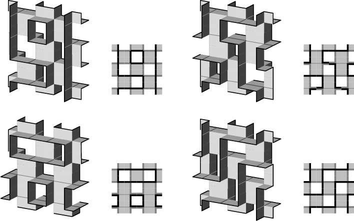
We can combine monkey-saddle and screw vertices in an astounding variety of ways. To generate a cubic polyhedron from any of the complexes in figure 5, we can repeatedly reflect across the front and back bounding planes, and translate vertically and to the right and left. These examples are meant to suggest that the full class of cubic polyhedra is quite large and varied.
We introduce some graphical notation to help discuss examples.
Given a cubic polyhedron , we use a planar diagram to
illustrate a slice through along some oriented plane in the cubic
lattice. A planar diagram will have shaded squares corresponding to
the faces of in , black edges corresponding to the faces of
incident to from above, and grey edges corresponding to the faces of
incident to from below. So for example,
a monkey-saddle vertex will always appear (up to congruence)
as
![[Uncaptioned image]](0205145v1/ad.png) , and a screw vertex will appear (up to congruence)
as either
, and a screw vertex will appear (up to congruence)
as either
![[Uncaptioned image]](0205145v1/bd1.png) or
or
![[Uncaptioned image]](0205145v1/bd2.png) ,
depending whether or not the axis of the vertex
is normal to the plane of the diagram.
Figure 5 also shows planar diagrams for the examples.
,
depending whether or not the axis of the vertex
is normal to the plane of the diagram.
Figure 5 also shows planar diagrams for the examples.
1.5 Configurations around a face in a cubic polyhedron
Let be a (square) face, which we think of as horizontal, in a cubic polyhedron . Each of the four edges of is either a crease or a flange, but successive edges cannot both be flanges, because the vertex between them would then have two perpendicular flanges. Furthermore, if there are successive creases, the neighboring squares across them have to alternate up and down (from the plane of ). We deduce that a (partial) planar diagram in the plane of must look like one of the four possibilities in figure 6.

We say that is a normal face of if no adjacent faces are coplanar with , that is, if all its edges are creases. The four adjacent faces across these creases must alternate up and down. (This is the first case in figure 6.) The complete configuration of in a neighborhood of is then given (up to isometry) by one of the six planar diagrams in figure 8.


To see this, consider how monkey-saddle and screw vertices (whose axes
must be vertical) occur in cyclic order around .
There are a priori six possibilities:
![[Uncaptioned image]](0205145v1/d1.png) ,
,
![[Uncaptioned image]](0205145v1/d2.png) ,
,
![[Uncaptioned image]](0205145v1/d3.png) ,
,
![[Uncaptioned image]](0205145v1/d4.png) ,
,
![[Uncaptioned image]](0205145v1/d5.png) , and
, and
![[Uncaptioned image]](0205145v1/d6.png) ,
where these dot diagrams record the types of vertices
in a slice through by dots on the integer lattice, with
unfilled dots
,
where these dot diagrams record the types of vertices
in a slice through by dots on the integer lattice, with
unfilled dots
![[Uncaptioned image]](0205145v1/adot.png) for vertices and filled dots
for vertices and filled dots
![[Uncaptioned image]](0205145v1/bdot.png) for screw vertices. For each of these six possibilities,
the fact that the central square is normal means that there is
a uniquely determined configuration as in figure 8.
for screw vertices. For each of these six possibilities,
the fact that the central square is normal means that there is
a uniquely determined configuration as in figure 8.
A face of which is not normal has, among its edges, either one flange or two opposite flanges. If there is one flange, it is the horizontal axis connecting two screw vertices. The other two vertices of can be either monkey-saddles or screws (with vertical axis); the three resulting configurations are shown in figure 8.
A face with two (opposite) flanges among its edges must be in one of the last two configurations shown in figure 6. Note that the second one, where each flange connects two screws of the same handedness, is the unique configuration of a face with two opposite creases bent to different sides:
Lemma 1.4
Suppose a face in a cubic polyhedron has two opposite edges which are creases, and the two adjacent faces across these edges lie on opposite sides of the plane containing . Then the other two edges of are flanges, and each of them is the common axis of two successive screw vertices of equal handedness.
We will not illustrate the nine possible diagrams around
a missing square in a cubic polyhedron. Note, however, that
if all four edges are creases, there are four configurations,
corresponding to the dot diagrams with even numbers of black (or white) dots.
In particular, the diagrams
and
cannot occur around a missing square.
The local configuration around a normal face is a box in one of the six configurations shown in figure 8. We define a tower to be one of the (six) configurations obtained from these by reflections.
Lemma 1.5
Given a configuration in a vertical box, if all the central horizontal squares are present as normal faces in , then is a tower.
Proof Each layer of is one of the six local configurations around a normal face. But each one of these can stack vertically only to its mirror image. So must be generated by reflections from any of its layers.
2 Screw vertices in cubic polyhedra
Because monkey-saddles do not have flanges, the flanges of any screw vertex in a cubic polyhedron must connect to further screws along the axis. Therefore, any screw vertex lies in a bi-infinite column of screws with a common axis line. Such a column is specified by a sequence specifying the handedness of each vertex. (Shifting or reversing the sequence results in a directly congruent column; interchanging and results in a reflected column.)
Lemma 2.1
There are uncountably many cubic polyhedra with all screw vertices.
Proof For any sequence , the column is a configuration in a box, which can be reflected to a complete cubic polyhedron by Lemma 1.1. (See figure 9.) These polyhedra are congruent only when the corresponding columns are.


When two adjacent vertices in a column have the same handedness, we say the column has a twist along the flange joining them; the normal of a twist is the normal direction to that flange (and the bi-axis is the direction perpendicular to both the axis and the normal).
Let be the alternating sequence . Then is the unique untwisted column, and is the polyhedron we saw in the introduction.
Note that each divides into two congruent regions. To see this, shift any by ; this interchanges the components of the complement of , but leaves invariant. (The polyhedron also divides space into two congruent regions, as seen by a body diagonal translation.)
If we (repeatedly) reflect a column in one coordinate direction but not the other, we get a box which we call the slab ; see figure 9. (We can also fill out a box with reflected monkey-saddles; we call this configuration a sheet.)
The axis of a slab is the direction of the axis line in any of its columns, and its normal is its direction of finite extent. (Again, the bi-axis is the direction perpendicular to both the axis and the normal.) Note that if two slabs in a cubic polyhedron intersect, they do so in a common column, and thus they have the same axis direction. Any slab is invariant under translation by two units along its bi-axis, because it was generated by reflections in planes a unit distance apart.
We now construct a second uncountable family of cubic polyhedra, indexed by a bi-infinite ternary sequence . The polyhedron is built from layers in horizontal planes. If , then there is a sheet of monkey-saddles in the plane ; otherwise there is an untwisted slab oriented to have normal and axis . (Because is untwisted, it fits against a copy of itself with or without a rotation, or against a sheet, as illustrated in figure 10.)

Lemma 2.2
Two adjacent parallel columns must be reflections of each other.
Proof If two adjacent screw vertices have the same handedness, then either they share an axis in a common column, or they have perpendicular axes. In two adjacent parallel columns, corresponding vertices thus have opposite handedness, and are mirror images by Lemma 1.2.
Lemma 2.3
Three mutually perpendicular untwisted columns cannot be mutually adjacent.
Proof Two adjacent perpendicular columns touch in screws of the same handedness, but handedness alternates along any untwisted column.
Lemma 2.4
Let be a column of screws in a cubic polyhedron . If has a twist, then lies in a slab with the same normal as that twist. Moreover, if has a pair of twists separated by an odd distance, is congruent to some , with all screw vertices.
Proof Suppose there are two successive screws of the same handedness in a column . The edge connecting them is their common axis, a flange between two coplanar faces and . (See figure 11.) But each is then of the type described by Lemma 1.4, so its opposite edge is similarly a twist in a column parallel to .
If a column has twists with odd separation distance, then their normals are perpendicular. Applying the argument above, adjacent to in any direction there must be a mirror-image column. Repeating, we see that our polyhedron must be .

Consequently, if is a slab in a polyhedron other than , the sequence must be formed by pairs and ; since twists correspond to consecutive vertices of the same handedness, this ensures all twists lie an even distance apart.
Lemma 2.5
Suppose is a cubic polyhedron containing a twisted slab . Unless , every slab in has the same normal as .
Proof Any slab with a different normal would intersect along a twisted column ; let be the normal direction to some twist in . Both slabs and have the same axis (along ) but distinct normals; let denote the one whose normal is not equal to . The consecutive columns in the slab are reflections of one another, so they all are twisted and have normal . By Lemma 2.4, each lies in a slab with normal , so .
Lemma 2.6
Let be a cubic polyhedron with all screw vertices such that there is some column in with a twist. Then all columns in are parallel, and is congruent to some .
Proof Let be a column with a twist between vertices and . By Lemma 2.4, lies in some slab with the same normal as that twist. Consider the vertices adjacent to in that normal direction. If either is , then it is a reflection of , with axis parallel to that of , so we get a parallel column. Then this column is also in a slab, and propogating this argument, we have the desired result.
But the cannot both be , for then each would have axis perpendicular to that of . But then and would be adjacent vertices with parallel axes, contradicting Lemma 2.2.
Theorem 2.7
Any polyhedron with all screw vertices is congruent to a or a .
Proof Let be a cubic polyhedron with all screw vertices. The vertices of the cubic lattice are partitioned into columns, which clearly can have axes in at most two directions. We may assume each column is untwisted, for otherwise the last lemma would apply. If all the axes are parallel, then is congruent to some by Lemma 2.2. Otherwise, we can at least partition the vertices into planes, within which all axes are parallel. Within each plane, the (untwisted) columns form a slab congruent to . The family includes all possible ways for these untwisted slabs to fit together, so we are done.
Note that any cubic polyhedron which is uniform in the sense of having regular faces and a symmetry acting transitively on the vertices must either be or have all screw vertices and be some or , where the sequences and must have transitive symmetry group. The possibilities (up to isometry) are exactly
Of course, is the uniform polyhedron already mentioned. The four others, , , and , are additional new uniform polyhedra, shown in figure 12. Of course, any all-screw polyhedron in the uncountable families and is semi-regular in the weaker sense of having regular faces and congruent vertex figures.

3 Operations on cubic polyhedra
In order to understand cubic polyhedra that mix monkey-saddle and screw vertices, we next define two operations. Pushing a tower changes monkey-saddle vertices to screw vertices (and vice versa) within the four columns of the tower. Inserting a slab cuts a polyhedron along an appropriate plane, moves the two pieces apart, and adds a new slab of screws between them. Our Main Theorem 4.5 will say that applying these operations in turn, starting from , suffices to create any generic cubic polyhedron.
3.1 Pushing towers
Remember that a tower is one of six possible configurations in a box obtained by mirror reflection from the local configuration around a normal face. Typical towers are shown in figure 13. Of course, a screw vertex in a tower is part of a column contained in the tower. Note also that the vertical faces within a tower are present or absent in checkerboard fashion.
Given a tower in a cubic polyhedron , we push the tower by moving each face within the tower one unit along the axis of the tower. Since all horizontal faces are present in the configuration, we need not worry about them. So we can equivalently describe the push as removing all the vertical faces within the tower and filling in vertical faces where before there were none. In figure 13 we show the result of pushing on each diagram from figure 8. The following lemma should be clear:
Lemma 3.1
The result of pushing any tower is again a cubic polyhedron. After pushing, monkey-saddle vertices in the tower become screw vertices and vice versa.

As an exercise, we note that each polyhedron in figure 5 can be created by applying tower pushes to , except the one in the upper right. (That one has no towers, and can be described instead by the techniques below.)
The columns within a tower are untwisted. Conversely, the following lemma shows that it is not hard to find towers around untwisted columns.
Lemma 3.2
Suppose is a cubic polyhedron, and is a normal face of at least one of whose vertices is a screw lying in an untwisted column. Then is in a tower with axis along the normal to .
Proof The local configuration around looks like one of the six configurations in figure 8. The first of the six is ruled out, as it has only vertices. Let be a screw vertex of , call its axis direction (normal to ) vertical, and assume without loss of generality that is an vertex. Above and below are vertices , since this column has no twists. Thus there are parallel faces in just above and below . Since the edges of incident to are both creases, the configuration near looks like one of the diagrams in figure 8 or 8. But none of the possibilities with flanges (figure 8) can fit above or below the normal face . Thus must also be normal, and in fact mirror images of . Continuing in this way, we find the configuration to be part of a tower.
Lemma 3.3
Let be any cubic polyhedron, and be any column of screw vertices in . If does not lie in a slab or in a tower, then lies sandwiched between two slabs whose parallel axes are perpendicular to the axis of .
Proof
If the column has a twist, it lies in a slab.
So suppose is untwisted, and call its axis direction vertical.
If, among the horizontal faces incident to , one is normal,
the previous lemma applies, and is part of a tower.
Thus, we may assume that every horizontal slice through is in
the configuration
![[Uncaptioned image]](0205145v1/tbetween.png) .
But then the screw vertices to either side of
must lie in slabs, for they lie in columns with axes
(the thin black lines) perpendicular to that of ,
and such columns must occur at every level of .
Therefore the column lies between two slabs, as desired.
(It is possible that is also part of a slab itself.)
.
But then the screw vertices to either side of
must lie in slabs, for they lie in columns with axes
(the thin black lines) perpendicular to that of ,
and such columns must occur at every level of .
Therefore the column lies between two slabs, as desired.
(It is possible that is also part of a slab itself.)
Our Main Theorem 4.5 will say that any cubic polyhedron either is a or is obtained from a by pushing some towers and then inserting slabs.
Let us consider how to apply tower pushes to a . The polyhedron has a checkerboard of towers in each coordinate direction. Any other has slabs with horizontal axis, and thus has no vertical towers. We find horizontal towers at any level except where alternates from to . The set of horizontal towers is always nonempty, except in .
If we are starting with , we first push any (infinite, finite or empty) subset of the vertical towers. (A nontrivial push will create some flanges and thus destroy some horizontal towers, but it may also create new ones.)
We now take the resulting polyhedron (or our starting ) and push any subset of its towers in the -direction. (Note that if we push a tower at a level where had a or , we will destroy the slab at that level.) Finally, we push any subset of the remaining towers in the -direction.
We call any cubic polyhedron resulting from this procedure a pushed-.
3.2 Removing and inserting slabs
Given a cubic polyhedron , we remove a slab by the following operation: delete the slab completely, and then join the two (half-space) components of the complement together by translating one of them by one unit along the slab normal (to bring them together) plus one unit along the slab bi-axis (to let them match). For example, in figure 14 we show the result of removing a slab from the cubic polyhedron partly indicated by the planar diagram. It is not hard, using such diagrams, to prove the following:
Lemma 3.4
Let be a cubic polyhedron containing a slab ; the result of removing is again a (well-defined) cubic polyhedron.

We define inserting a slab to be the inverse of this operation. After the next lemma, we will explain exactly what we mean by inserting an infinite sequence of slabs, but we note now that any can be obtained from by inserting (perhaps infintely many) untwisted slabs.
We will now examine the conditions under which a slab can be inserted into a pushed-, and will find that the slab to be inserted is usually uniquely determined.
Lemma 3.5
Let be a pushed-. If has columns in all three directions, no slab can be inserted in . If has no vertical columns, then slabs can be inserted at any horizontal plane , .

Proof If has columns in all three directions, then any plane is cut perpendicularly by the axis of some column, and thus cannot be a candidate for slab insertion.
If there are no vertical columns, consider a horizontal plane given by . We will refer to the intersection of with as the pattern of in . This shows us the set of faces in which are bisected by , and is always a union of squares. If we insert a slab along , the boundary of the slab must have the same pattern.
If is a , the pattern we see is always the trivial pattern consisting of a square array of squares, as in figure 15 (left). (This is why the three possible layers in a can fit together in any order.)
To determine the pattern of in , we need only look at which tower pushes in the plane have been performed. (Note that horizontal tower pushes which occur one layer higher or lower in will change the vertices just above and below , but won’t affect the faces cut by or thus what slab we can insert. Also, depending on , pushes in may or may not be possible.)
If any tower within has been pushed, then all tower pushes at that level (or at levels just above and below ) must have parallel axes. The only exception is that if all -towers within are pushed, then we again see the trivial pattern in (shifted by one unit), and any subset of the (new) -towers in can be pushed.
If the pattern of in is trivial (meaning that either no towers or all towers in have been pushed), we can insert an untwisted slab with axis or . Indeed, we can insert any finite number of untwisted slabs, indexed by a finite sequence of ’s and ’s, or we can delete the half-space of to one side of and insert a half-space of some corresponding to an infinite sequence of ’s and ’s. Of course, the result of such an insertion is merely another pushed-.
On the other hand, if the pattern is nontrivial, then all tower pushes have occurred with parallel axes, say along , and are at an even distance apart from one another within . We now define a bi-infinite sequence of letters : reading along the -direction in , each tower with axis in the -direction was either npushed or ushed. The substitution rules , convert to a sequence . Then the unique slab that can be inserted along is , as illustrated in figure 15. Moreover, we can insert any finite number of ’s, each a reflection of the next, or we can delete the half-space to one side of and insert a half-space of .
If is a pushed- with no vertical columns, we can now explain what we mean by insertion of a (possibly infinite) set of slabs. Beginning near the origin and working outwards, we examine the planes , for . If a given plane has the trivial pattern, we can insert any finite or infinite sequence of untwisted slabs, indexed by choice of axis, or . Otherwise, there is a sequence associated with the plane, as described in the proof of Lemma 3.5, and we can insert any finite or infinite number of copies of . (To insert an infinite sequence of slabs at one level, we throw out the half-space bounded by the plane away from the origin, and then stop the procedure on that side.) In our Main Theorem 4.5, we will show that any cubic polyhedron can be obtained from a pushed- in this way.
4 Classifying Cubic Polyhedra
We now show that, given any cubic polyhedron, we can apply the operations of the previous section in reverse to simplify it. First we consider cases where tower pushes alone can bring us back to .
Lemma 4.1
Let be a cubic polyhedron in which all columns (if there are any) are untwisted with vertical axis. Then can be obtained from by pushing some set of vertical towers.
Proof The polyhedron must be generated by reflection from any box around a horizontal plane , since the screws lie in untwisted vertical columns and the monkey-saddles also lie in infinite vertical lines. It follows that every horizontal face in is normal and part of a vertical tower.
We will assign a parity modulo to each tower as follows.
Arbitrarily assign parity to one tower, centered at some point .
We may assume that the planar diagram in at this tower
is
![[Uncaptioned image]](0205145v1/towdiag1.png) . Any other tower is centered at
some with .
To this tower we assign parity
if it has the same diagram
, and parity
if it has the other diagram
. Any other tower is centered at
some with .
To this tower we assign parity
if it has the same diagram
, and parity
if it has the other diagram
![[Uncaptioned image]](0205145v1/towdiag2.png) .
Note that two adjacent towers intersect in a column of screws
if they have opposite parity, as in
.
Note that two adjacent towers intersect in a column of screws
if they have opposite parity, as in
![[Uncaptioned image]](0205145v1/oppparity.png) ,
while they intersect in a line of monkey-saddles if they have
the same parity, as in
,
while they intersect in a line of monkey-saddles if they have
the same parity, as in
![[Uncaptioned image]](0205145v1/sameparity.png) .
.
Pushing a tower switches its parity and leaves all other towers unaffected. So we now simply push all towers of parity ; this leaves all towers with the same parity, so we now have all monkey-saddle vertices, as desired.
Lemma 4.2
Let be a cubic polyhedron with columns in all three coordinate directions. Then we can push some set of vertical towers to eliminate all vertical columns. All columns in the resulting polyhedron are untwisted and horizontal, and has at least one vertical tower (of monkey-saddles).
Proof There can be no slabs in , and thus all columns are untwisted. We will first find pushes to remove all vertical columns.
Choose any horizontal plane in the cubic lattice, and consider the set of all screw vertices in with horizontal axis. Since these lie in horizontal columns, the projection of to consists of infinite lines of vertices, including at least one line in each direction. Its complement (within the set of all vertices in ) is a (possibly infinite) union of rectangular regions. Each region is finite or singly infinite in each direction, and thus has connected boundary.
In figure 16 we illustrate a schematic of the slice in .
Somewhere above or below each occurence of the symbol
![[Uncaptioned image]](0205145v1/abovebdot.png) there is a screw vertex with horizontal axis.
At the locations marked
there is a screw vertex with horizontal axis.
At the locations marked
![[Uncaptioned image]](0205145v1/aorbdot.png) there is either a monkey-saddle
vertex
or a screw vertex with vertical axis
.
there is either a monkey-saddle
vertex
or a screw vertex with vertical axis
.

Now consider some rectangle of vertices in the complement of the projection of , and assume . The configuration around is a box which necessarily appears reflected in to fill out a box. (Indeed, any screw vertex in is part of an untwisted vertical column, and any monkey-saddle vertex lies above and below further monkey-saddles by the definition of .)
We will prove that we can push vertical towers within to eliminate all screw vertices in . Within , horizontal faces appear in a checkerboard pattern, as seen in figure 17. Those along the boundaries of (shown in lighter gray in the figure) are not in towers, since they are incident, at some level, to horizontal screws in . But all interior horizontal faces (in darker gray) lie in vertical towers, by Lemma 3.2 and the definition of .
Since has no slabs, by Lemma 3.3 any column of screws must be in a tower. If then there are no towers in , so there can be no screws in , and we are done.
We now assume ; we will return later to the case . Note that interior vertices of are incident to exactly two towers, while vertices along an edge are incident to exactly one. A corner vertex in is incident to either one tower or zero towers, depending on whether or not there is a horizontal face in that corner of .
We assign a parity modulo to each tower in exactly as in the proof of Lemma 4.1, and then push all towers of parity . Again, this leaves all towers within with the same parity, meaning that the interior of has only monkey-saddle vertices. (Beginning with any polyhedron represented by the first configuration in figure 17, we have now obtained the second one.)


If all boundary vertices of are also now monkey-saddles (as in the third configuration in figure 17), we have proved the claim, having eliminated all vertical columns from this portion of the cubic polyhedron.
Otherwise, we claim that each screw vertex in is incident to exactly one tower, while each monkey-saddle is incident to zero or two towers. (This is the case in the last configuration in figure 17.) Then pushing all towers in will remove all vertical columns, as desired. (In other words, if we originally had pushed the towers of parity instead of those of parity , we would have obtained all monkey-saddles.) The claim is equivalent to saying that there are screws along the edges of , and screws in corners where a horizontal face is present, but monkey-saddles in the other corners.
Suppose there is a screw in an inappropriate corner, that is,
we see the configuration
![[Uncaptioned image]](0205145v1/forbid3.png) .
At some levels above or below , there are horizontal
columns along one edge of ; at other levels there are perpendicular
horizontal columns along the other edge of .
But these two possibilities cannot happen at successive levels,
since then we would have
three mutually perpendicular and adjacent untwisted columns,
contradicting Lemma 2.3.
This means that at some intermediate levels, we have
monkey-saddles at all three positions marked
.
This means we see the configuration
.
At some levels above or below , there are horizontal
columns along one edge of ; at other levels there are perpendicular
horizontal columns along the other edge of .
But these two possibilities cannot happen at successive levels,
since then we would have
three mutually perpendicular and adjacent untwisted columns,
contradicting Lemma 2.3.
This means that at some intermediate levels, we have
monkey-saddles at all three positions marked
.
This means we see the configuration
![[Uncaptioned image]](0205145v1/forbid1.png) ,
which is impossible as we noted in Section 1.5.
,
which is impossible as we noted in Section 1.5.
Remember we have assumed there is at least one screw on the boundary of .
We cannot have the configuration
![[Uncaptioned image]](0205145v1/forbid7.png) , since, again,
at some level we will have monkey-saddle vertices at the positions
marked
and thus would have the forbidden
configuration . Similarly, we cannot have
the configuration
, since, again,
at some level we will have monkey-saddle vertices at the positions
marked
and thus would have the forbidden
configuration . Similarly, we cannot have
the configuration
![[Uncaptioned image]](0205145v1/forbid8.png) , for there are only monkey-saddles
in the (non-empty) interior of ,
and again we find the forbidden configuration .
Thus, along an edge of with one screw vertex,
we continue to see screws until we reach a corner.
, for there are only monkey-saddles
in the (non-empty) interior of ,
and again we find the forbidden configuration .
Thus, along an edge of with one screw vertex,
we continue to see screws until we reach a corner.
Finally, we check that we cannot have a monkey-saddle at an
inappropriate corner: we cannot see the configuration
![[Uncaptioned image]](0205145v1/forbid9.png) ,
for again at some level the positions marked
must be monkey-saddles, giving yet again.
,
for again at some level the positions marked
must be monkey-saddles, giving yet again.
So all corners must have the appropriate vertices,
either
![[Uncaptioned image]](0205145v1/bcorner.png) or
or
![[Uncaptioned image]](0205145v1/acorner.png) .
In the latter case, we cannot have the configuration
.
In the latter case, we cannot have the configuration
![[Uncaptioned image]](0205145v1/forbid10.png) ,
since we have only monkey-saddles
in the interior of , giving once again.
Therefore, since the boundary of is connected and
contains at least one screw,
it consists entirely of screws
(except monkey-saddles in the appropriate corners).
,
since we have only monkey-saddles
in the interior of , giving once again.
Therefore, since the boundary of is connected and
contains at least one screw,
it consists entirely of screws
(except monkey-saddles in the appropriate corners).
Finally, suppose . At the end of , we must see one of
the configurations at the left in figure 18.
Note that the configuration
![[Uncaptioned image]](0205145v1/forbid2.png) is forbidden
just like .
Since we cannot have either or , by induction the towers in the
interior of must consist of a sequence of the two configurations
in the middle in figure 18, and the vertices of each tower
are either all screws or all monkey-saddles. Moreover, each
vertex in belongs to just one tower. We simply push the towers
that consist of screw vertices and leave the others alone. We are
left with all monkey-saddles in .
is forbidden
just like .
Since we cannot have either or , by induction the towers in the
interior of must consist of a sequence of the two configurations
in the middle in figure 18, and the vertices of each tower
are either all screws or all monkey-saddles. Moreover, each
vertex in belongs to just one tower. We simply push the towers
that consist of screw vertices and leave the others alone. We are
left with all monkey-saddles in .

If we repeat the procedure described so far for each rectangle , we can push towers to eliminate all screws with vertical axis, and obtain the polyhedron . It contains no vertical columns, but does contain the vertical towers we pushed in order to obtain it from .
Lemma 4.3
Let is a cubic polyhedron with no vertical columns and no slabs. Then is a pushed-. If includes a vertical tower (of monkey-saddles), then it is actually a pushed-.
Proof If has columns only in a single direction, we can apply Lemma 4.1. So suppose has columns along both and . The proof will be very similar to the previous one.
Let be the -plane, and the set of screws with axis in the -direction. Projecting to , we now find that the complement is a union of horizontal strips . When , since has no slabs, Lemma 3.3 again guarantees that the region contains no screws. So we may assume .
First, we will suppose that does include a vertical tower. This tower gives a vertical strip (of width ) in which we see only monkey-saddles. The complement of in each is two semi-infinite strips . Each of these regions has corners and connected boundary, as in the previous proof.
The argument then proceeds as before, with the monkey saddles along playing the same role as the monkey-saddles we earlier found at some level along each boundary of . We assign parities to the towers in , and push the towers of parity . Then if any screws remain along the boundary, we push all towers. The same arguments guarantee that this removes all columns from .
Repeating for each region , we eventually remove all columns along . We can then use Lemma 4.1 to remove the remaining columns (along ).
If contains no vertical tower, the argument is a bit more difficult. We work directly on the strips of height . First assume . Assign parities to the towers in , and push those of parity . Fix one boundary component of ; the usual arguments imply that along this boundary now either all vertices are screws or all are monkey-saddles. If both boundary components have screws, push all towers in to eliminate all the screws. However, if one boundary has screws and the other has monkey-saddles, there is no way to push towers to get rid of all screws; we are left with a slab (untwisted, with axis and normal ) along this boundary of .
If , the situation is similar. Again, since we cannot have the configurations or , the towers in either are a sequence of the two configurations in figure 18 (center) or are a sequence of the two configurations figure 18 (right). In the first case, we push the towers consisting of all screw vertices as before, removing all columns from . In the second case, we push all copies of the far-right configuration. (In either case, the push we use is in fact the usual push of all towers of parity , although the accounting is more difficult here.)
In summary, within in each region , we push towers to eliminate all columns with axis except, perhaps, for a single untwisted slab along one boundary of . We arrange (by pushing all towers in if necessary) that these slabs are always at the top of each region . It follows that these slabs are separated by distance at least from each other (since each was at least units high, and they are separated by at least one layer). Call the resulting cubic polyhedron .
Because of these slabs, we cannot now apply Lemma 4.1 to . We could remove the slabs and then apply that lemma. This would show our original could be obtained from by a combination of tower pushes and slab insertions, but would not demonstrate that it is a pushed-.
Instead, we repeat the argument we have just given, but with the roles of and interchanged, starting from . We must be careful because does contain slabs. But we get for each strip directly, since the slabs (the only screws with axis ) are separated vertically by units.
We get rid of internal columns in by pushing towers of parity
as usual. Along a boundary of , we again claim that either all
vertices are screws or all are monkey-saddles. We can no longer
find some height above at which there are monkey-saddles
just outside , since is now bounded by slabs.
But these slabs are untwisted so the configuration
is still forbidden, and the argument goes through as before.
We can thus find tower pushes in the direction taking to a polyhedron with no columns except untwisted horizontal slabs. This is a . So , and then our original , is a pushed-.
Corollary 4.4
Let be a cubic polyhedron with no slabs. Then is a pushed-.
Proof The columns of must be untwisted. If they have parallel axes, apply Lemma 4.1. If they occur in two directions, apply Lemma 4.3. If they occur in all three directions, apply Lemma 4.2 and then Lemma 4.3.
Main Theorem 4.5
Any cubic polyhedron is a or is obtained by inserting slabs into some pushed-.
Proof If a cubic polyhedron has all screw vertices, then it is a or a , and we are done.
Otherwise, the slabs in do not fill out all of . Suppose there are two slabs in with different normals. They intersect along a column which we will call vertical. All columns must be vertical, since a horizontal column would cut one of the slabs. By Lemma 2.5 all columns are also untwisted (or we would have a ). Thus Lemma 4.1 applies to show is a pushed-.
Thus we may assume all slabs in have the same normal. Call this normal direction vertical and the slabs horizontal. We can remove all slabs; we are left with an box , with being bi-infinite, infinite or finite depending on whether there were originally zero, one or two half-spaces of slabs. We reflect if necessary to get a complete cubic polyhedron with no slabs, from which can be obtained by inserting slabs. Now Corollary 4.4 applies to , showing is a pushed-, as desired.
5 Discrete Minimal Surfaces in the Cubic Lattice
As we mentioned in the introduction, a complete surface built from faces of the cubic lattice is discrete minimal if and only if each vertex of the lattice has one of five possible configurations of faces. We call these , , , and , where , and are the vertex configurations of cubic polyhedra, represents a flat vertex with four coplanar squares, and is an empty vertex, not in the polyhedron. It would be interesting to extend our classification theorem to give a complete list of all such discrete minimal surfaces; we give a few partial results here.
First, let us give some examples. A trivial family, indexed by subsets of , contains any collection of horizontal planes. These surfaces are not connected, and do not include every vertex in the cubic lattice.
We can construct a more interesting example as follows: Attach infinite sequences of flat vertices to the two flanges of a screw vertex, and then extend this box to a complete surface by reflection. This is clearly a discrete version of Scherk’s doubly periodic minimal surface, and it does relax to that surface. (See figure 19.) In this polyhedron, there are two half-spaces containing stacked half-planes of flat vertices, separated by a layer of screw vertices which twist the half-planes 90 degrees. This polyhedron is connected, and does include every lattice vertex.


Lemma 5.1
Along the normal line of a flat vertex (or any coordinate line through an empty vertex) we find only empty vertices or flat vertices with that normal line.
Proof The empty and flat configurations are the only ones which omit edges, and they omit edges in colinear pairs. Thus all edges along any such line are omitted in the polyhedron.
Although this lemma constrains how flat vertices can appear, there is still more flexibility than for cubic polyhedra. For instance, a flat vertex can be surrounded on all four sides by screw vertices, as in figure 20. This block can be extended by reflection.


We will not attempt here to give a complete classification of all the discrete minimal surfaces in the cubic lattice.
References
- [1] T.F. Banchoff, Tightly Embedded -Dimensional Polyhedral Manifolds, Amer. J. Math., 87 (1965), 462–472.
- [2] K.A. Brakke, The Surface Evolver, Experimental Math. 1:2 (1992), 141–165.
- [3] H.S.M. Coxeter, Regular Polytopes, third edition, Dover (1973).
- [4] L. Hsu, R. Kusner and J.M. Sullivan, Minimizing the Squared Mean Curvature Integral for Surfaces in Space Forms, Experimental Math. 1:3 (1992), 191–207.
- [5] H. Karcher and K. Polthier, Construction of triply periodic minimal surfaces, Philos. Trans. Roy. Soc. London Ser. A 354 (1996), 2077–2104.
- [6] U. Pinkall and K. Polthier, Computing Discrete Minimal Surfaces and Their Conjugates, Experimental Math. 2:1 (1993), 15–36.