The Computational Complexity of Knot Genus and Spanning AreaThanks: Partially supported by ARC grant 420998.Thanks: This work was carried out while the second author was visiting the Institute for Advanced Study, partially supported by NSF grant DMS-0072348, and by a grant to the Institute for Advanced Study by AMIAS.Thanks: Third author partially supported by NSF grant DMS-9704286.
Abstract.
We show that the problem of deciding whether a polygonal knot in a closed three-dimensional manifold bounds a surface of genus at most , is NP-complete. We also show that the problem of deciding whether a curve in a PL manifold bounds a surface of area less than a given constant is NP-hard.
Key words and phrases:
Computational topology, complexity, knot, 3-manifold, NP-complete, normal surface, genus1991 Mathematics Subject Classification
Primary 11Y16, 57M50; Secondary 57M251. Introduction
In this paper we investigate the computational complexity of some problems in three-dimensional topology and geometry. We show that the problem of determining a bound on the genus of a knot in a 3-manifold, is NP-complete. Using similar ideas, we show that deciding whether a curve in a metrized PL 3-manifold bounds a surface of area less than a given constant is NP-hard.
Determining whether a given knot is trivial or not is one of the historically central questions in topology. The problem of finding an algorithm to determine knot triviality was posed by Dehn [1]. Dehn’s investigations into this area led to the formulation of the word and isomorphism problems, which played an important role in the development of the theory of algorithms. The first algorithm for the unknotting problem was given by Haken [3]. Haken’s procedure is based on normal surface theory, a method of representing surfaces introduced by Kneser [14]. Analysis of the computational complexity of this algorithm is more recent. Hass, Lagarias and Pippenger showed that Haken’s unknotting algorithm runs in time at most , where the knot is embedded in the 1-skeleton of a triangulated manifold with tetrahedra, and is a constant independent of or [5]. It was also shown in [5] that the unknotting problem is in NP.
The notion of genus was defined by Seifert [23] in 1935 for knots in the 3-sphere, and extends directly to knots in an arbitrary 3-manifold . Given a knot , consider the class of all orientable spanning surfaces for . These are surfaces embedded in with a single boundary component that coincides with . Seifert showed that this class is non-empty for any knot in the 3-sphere. For knots in a general manifold, is non-empty when represents a trivial element in the first integer homology group of . The genus of a knot is the minimum genus of a surface in , or if . The genus measures one aspect of the degree of “knottedness” of a curve.
The unknotting problem is a special case of the more general problem of determining the genus of a knot in a 3-manifold. Given a knot in an orientable 3-manifold and a positive integer , this problem asks for a procedure to determine whether the knot genus of , the minimal genus of an orientable spanning surface for in a 3-dimensional manifold, is at most . A knot is trivial, or unknotted, precisely when its genus is zero. We will show that the problem of determining the genus of a knot in a 3-manifold is NP-complete. Previous results on this problem were given in [5], where it was shown to lie in PSPACE, roughly the class of problems that run in polynomial space. No lower bounds on the running time were previously known.
We work with 3-manifolds that are triangulated and orientable, and with orientable embedded surfaces. This is not a significant restriction, since all compact 3-dimensional manifolds admit unique PL structures [15]. A knot in a triangulated 3-manifold is a connected simple (non self-intersecting) closed curve in the 1-skeleton of . Any smooth knot in a smooth manifold, or more generally any tame knot, is equivalent to a knot that lies in the 1-skeleton of some triangulation.
We formulate the problem of computing the genus as a language-recognition problem in the usual way, see [2]. In 1961 Schubert [21], in an extension of Haken’s work, showed the decidability of the problem:
| Problem: | 3-MANIFOLD KNOT GENUS |
| INSTANCE: | A triangulated 3-dimensional manifold , a knot in the |
| 1-skeleton of , and a natural number . | |
| QUESTION: | Does the knot have ? |
The size of an instance is measured by the sum of the number of tetrahedra in . In Section 3 we establish
Theorem 1.
3-MANIFOLD KNOT GENUS is NP-hard.
It was established in [5] that 3-MANIFOLD KNOT GENUS is in PSPACE. We improve this bound in Section 5 .
Theorem 2.
3-MANIFOLD KNOT GENUS is NP.
In combination these two results give:
Theorem 3.
3-MANIFOLD KNOT GENUS is NP-complete.
Theorem 1 is proved through a connection to ONE-IN-THREE SAT, a known NP-complete problem that will be reviewed in Section 3. The theorem carries out a construction that transforms an instance of ONE-IN-THREE SAT to an instance of 3-MANIFOLD KNOT GENUS. By “transform” we mean that an instance of one problem is changed to an instance of the second by a procedure that requires time polynomial in the size of the instance. To a boolean expression representing an instance of ONE-IN-THREE SAT we associate a positive integer and a certain knot in a triangulated, compact 3-manifold. This knot bounds a surface of genus at most exactly when there is a truth assignment to the boolean expression satisfying the requirements of ONE-IN-THREE SAT. Since ONE-IN-THREE SAT is NP-hard, this establishes that 3-MANIFOLD KNOT GENUS is also NP-hard.
In Section 5 we prove Theorem 2, giving a certificate which demonstrates in polynomial time that a genus knot bounds a surface of genus at most . The argument in [5] established that the unknotting problem is NP using the existence of a normal disk that lies along an extremal ray in the space of normal solutions, called a vertex surface in Jaco-Tollefson [11]. The existence of such an extremal normal surface of minimal genus spanning a knot is not known, so a new technique is needed (See [10] for known results here). This is provided in Theorem 12, which gives an algorithm to count the number of orbits of a type of pseudogroup action on a set. Theorem 12 seems likely to have more general applicability. In Section 4 we describe this algorithm and in Section 5 we apply it to a pseudogroup action that arises in the theory of normal surfaces. This allows us to determine in polynomial time the number of components in a normal surface described by an integer vector in . In particular we are able to certify that a normal surface is connected, orientable and has connected boundary. Since calculating the Euler characteristic of a normal surface can be done efficiently, establishing orientability and connectedness are the key steps in constructing a certificate of its genus.
In Section 6 we extend the orbit counting algorithm to allow the counting of additional integer weight sums associated to each orbit. This allows for the polynomial time calculation of the genus of all the components of a fundamental normal surface, as well as a count of the number of components.
The genus and the area of a surface are closely connected. In Section 7 we extend the methods developed in studying genus to study the problem of determining the smallest area of a spanning surface for a curve in a 3-manifold. We show that computing an upper bound on the area of a smallest area spanning surface is NP-hard.
We refer to [16] for a discussion of complexity classes such as NP and PSPACE and [25] for a discussion of complexity problems in low-dimensional topology.
Remarks:
- (1)
Knots are often studied in or rather than in a general manifold. Our methods show that determining knot genus in or , or any fixed manifold, is NP. It is not clear whether the corresponding problem remains NP-hard if one restricts consideration to knots in or .
- (2)
Casson has shown that a procedure to determine whether a 3-manifold is homeomorphic to the 3-sphere, following the 3-sphere recognition algorithm described in [18] and [24], runs in time less than , where is a polynomial. In the direction of lower bounds, it was shown in [13] that determining certain values of the Jones polynomial of alternating links is #P-hard.
We are grateful to the referee for numerous suggestions on the exposition of this paper.
2. Normal Surfaces
General surfaces in 3-manifolds can wind and twist around the manifold in complicated ways. Kneser described a procedure in which surfaces can be “pulled taut”, until they take a simple and rigid position [14]. In this normal position, they have very succinct algebraic descriptions. We use an approach to normal surfaces in triangulated 3-manifolds based on work of Jaco-Rubinstein [12] and Jaco-Tollefson [11]. A normal surface in a triangulated compact 3-manifold is a -surface whose intersection with each tetrahedron in consists of a finite number of disjoint elementary disks. These are properly embedded disks that are isotopic to either triangles or quadrilaterals as shown in Figure 1, by an isotopy preserving each face of the tetrahedron.
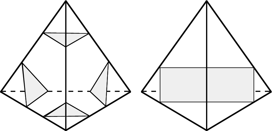
Within each tetrahedron of there are four possible triangles and three possible quadrilaterals, up to a normal isotopy of , an isotopy which leaves each cell of the triangulation of invariant. W. Haken observed that a normal surface is determined up to such isotopies by the number of pieces of each of the seven kinds of elementary disks that occur in each tetrahedron, or a vector in . A normal surface is described by a non-negative integer vector , that gives the normal coordinates of . There is a homogeneous rational cone in , called the Haken normal cone, that contains the vectors for all normal surfaces in .
If , then the Haken normal cone is specified by linear equations and inequalities of the form
The first set of equations expresses matching conditions, which say that the number of edges on a common triangular face of two adjacent tetrahedra, coming from a collection of elementary disks in each of the tetrahedra, must match. For each triangular face there are three types of edges (specified by a pair of edges on the triangle), which yield 3 matching conditions per face. Triangular faces in the boundary give no matching equations. The second set are called the positivity conditions. The cone is rational, because the above equations have integer coefficients. We let denote the set of integral vectors in the cone . An additional set of conditions, the quadrilateral conditions, is required for an integral vector in the cone to correspond to the normal coordinates of an embedded surface. This condition states that of the three types of quadrilateral found in each tetrahedron, only one can occur in the vector with non-zero coefficient. The quadrilateral conditions are required because two distinct types of quadrilateral in a single tetrahedron necessarily intersect, and we are interested in embedded, non-self-intersecting surfaces. A vector in the Haken normal cone that satisfies the quadrilateral conditions corresponds to an embedded normal surface. This surface is unique up to a normal isotopy. However it is important to note that the surface corresponding to a given vector in the cone may not be connected. A normal surface meets each edge of a triangulation in a finite number of points. The sum of these intersection numbers over all the edges of a triangulation is called the weight of the normal surface.
A fundamental normal surface is a normal surface such that
In the terminology of integer programming, such a vector is an element of the minimal Hilbert basis of , see Schrijver [20, Theorem 16.4]. A fundamental normal surface is always connected, but connected normal surfaces need not be fundamental. A vertex minimal solution is a special kind of fundamental surface, one that corresponds to a solution of the normal surface equations that lies along an extremal ray of the cone of solutions and is not a multiple of another such extremal solution. Hass, Lagarias and Pippenger [5, Lemma 6.1] gave a bound for the size of the vectors corresponding to any fundamental surface.
Theorem 4.
Let be a triangulated compact 3-manifold, possibly with boundary, that contains tetrahedra.
- •
Any vertex minimal solution of the Haken normal cone in has
- •
Any minimal Hilbert basis element of the Haken fundamental cone has
Schubert [21] showed that a surface of smallest genus spanning can be found among the fundamental surfaces.
Theorem 5.
There is a minimal genus spanning surface for which is a fundamental normal surface.
Similar to the theory of normal surfaces, though somewhat easier, is the theory of normal curves. These are curves on a surface that intersect each triangle in a collection of normal arcs, arcs that have endpoints on distinct edges. Normal curves arise as the boundaries of normal surfaces in a manifold with boundary. Since there are three such arcs in each triangle, normal isotopy classes of normal curves in a surface that contains triangles are described by integer vectors in .
3. 3-MANIFOLD KNOT GENUS is NP-hard
In this section we show how to reduce an instance of ONE-IN-THREE SAT to an instance of 3-MANIFOLD KNOT GENUS. Since ONE-IN-THREE SAT is known to be NP-hard, this establishes that 3-MANIFOLD KNOT GENUS is also NP-hard. The problem ONE-IN-THREE SAT concerns logical expressions involving collections of literals (boolean variables or their negations) gathered in clauses consisting of three literals connected with ’s. The logical expression contains a collection of clauses connected with ’s.
| Problem: ONE-IN-THREE SAT | |
| INSTANCE: A set of variables and a collection of clauses over | |
| such that each clause contains 3 literals. | |
| QUESTION: | Is there a truth assignment for such that each clause in |
| has exactly one true literal? |
Schaefer [19] established that ONE-IN-THREE SAT is NP-complete. To prove Theorem 1, establishing that 3-MANIFOLD KNOT GENUS is NP-hard, we show that an arbitrary problem in ONE-IN-THREE SAT can be reduced in polynomial time to a problem in 3-MANIFOLD KNOT GENUS. See Garey and Johnson [2] for a discussion and many examples of such reductions.
Let be a set of variables and be a set of clauses in an arbitrary instance of ONE-IN-THREE SAT. We will describe a knot in a compact 3-dimensional manifold (with no boundary) and an integer such that bounds a surface of genus smaller or equal to if and only if is satisfiable so that each clause in contains exactly one true literal. We construct the 3-manifold in stages. First we construct a 2-dimensional simplicial complex, then we thicken this complex, replacing triangles with subdivided triangular prisms, getting a triangulated, 3-dimensional manifold with boundary, as indicated in Figure 2. Finally we use a doubling construction, taking two copies of the manifold with boundary and gluing their boundaries together, to obtain a closed 3-manifold.

To begin, we form a type of singular surface , that we call a branching surface, by identifying boundary curves of a collection of surfaces with boundary, each forming what we refer to as a piece of the branching surface. We construct this collection of surfaces as follows. Let be the number of times that the variable appears in the collection of clauses, and be the number of times that the negation of appears. For , let and be genus one surfaces with and boundary curves respectively. Also set to be a planar surface with boundary curves. One of these boundary curves will later become the knot . The branching surface is constructed by identifying these surfaces along appropriate boundary components as indicated in Figure 3.

Branching occurs when more than two boundary curves are identified along a single curve. We identify pairs of boundary curves by giving a homeomorphism between them. Up to isotopy, this is determined by specifying an orientation on the curves and setting the homeomorphism to be orientation reversing. We first fix an orientation on each of and . This induces an orientation on each boundary curve. All identifications will involve gluing a boundary component of or to a boundary component of , and we require this gluing to be an orientation reversing homeomorphism. Label by the boundary components of . The boundary component of , which will become our knot, has nothing identified to it. For each , , one boundary curve from the surface is identified to . The remaining boundary components of are identified with of the curves on , with one component of identified with for each occurrence of the literal in the clause in . Similarly, one curve of is identified to the component of labeled , and the remaining boundary components are glued to , with a component glued to for each occurrence of the literal in the clause of . A total of three surface boundaries are identified along each of , and exactly four surface boundaries are identified along each of , as in Figure 3.
Lemma 6.
There is a truth assignment for such that each clause in has exactly one true literal if and only if there is a surface with connected boundary and genus at most and a continuous map such that is a homeomorphism onto .
Proof.
Suppose there is a truth assignment for such that each clause in contains exactly one true literal. Form a surface inside by taking the union of and either if is true, or if is false. Then exactly two boundary components will be identified along each of the boundary components of other than itself, and becomes the boundary of the resulting embedded surface . There is a contribution of one to the genus from each of the literals, since and each have genus one, and a contribution of one to the genus from each handle formed when a boundary component of a surface or is glued to along a curve . The genus of is therefore equal to .
Now suppose there is a surface of genus mapped continuously into that has a single boundary component mapped homeomorphically to the boundary curve . We will show in this case that there is a surface with the same boundary, consisting of certain pieces of identified along their boundaries, having genus precisely , and containing, along each curve , exactly one of the three pieces of surface joining .
The map of into may be quite complicated, winding back and forth across , but by standard transversality arguments we can homotop so that it is a union of homeomorphisms of subsurfaces of mapped homeomorphically to one of the pieces , , forming . More precisely, we can perturb by a small homotopy so that its intersection with the boundary components of is transverse, and pulls back to a collection of simple closed curves on . If any of these curves bounds a disk in , then the disk is mapped into some subsurface of while the boundary curve is mapped to . Since is not itself a disk, the disk can be homotoped into , and we can therefore homotop in a neighborhood of this disk to remove a component of . After repeating finitely many times, each component of the complement of in has non-positive Euler characteristic. The image of in each piece , , has an algebraic degree, which is either even or odd. This degree equals the number of pre-images in of a generic point in the piece. The degree of the map from on is odd, since is the boundary of and therefore maps an odd number of times to points near . The sum of the degrees along each of the pieces meeting a curve or is even, since has no boundary along these curves. In particular, for each , exactly one of , has odd multiplicity in . Form a new surface by taking the union of and each of the pieces , which have odd multiplicity in . We will show that . The surface is obtained from by a series of operations that either discard a subsurface with non-positive Euler characteristic or replace a subsurface of that maps with odd degree to some piece with a subsurface mapping homeomorphically to . The Euler characteristic of a discarded subsurface of is smaller or equal to that of the subsurface that replaces it, so in either case.
The collection of pieces among , that are in the image of can be attached to along common boundary curves among , forming a connected surface of genus . Finally, a connected surface with boundary is obtained by identifying pairs of curves in that are mapped to the boundary components . Each then has either two or four curves in mapped to it, so there are either one or two identifications made along each . The choice of which pairs to identify, in case there are four curves mapped to , is not important. The Euler characteristic of is the same as that of and , and therefore greater or equal to that of . So the genus of is at most that of , genus. Each identification of a pair of surface boundaries along contributes one to the genus of . There is at least one such identification along each of the curves , though there may be two if each of the three surfaces meeting along has multiplicity one in . So identification of curves along adds at least to the genus of , and it follows that genus(. Since we have seen that genus, equality must hold. Equality holds when exactly one of the three surface pieces meeting along has odd multiplicity for each . We then assign the value “TRUE” to a literal if is used in , and the value “FALSE” to if is used in . This gives a truth assignment to in which each clause in has exactly one true literal. ∎
To show that 3-MANIFOLD KNOT GENUS is NP-hard we reduce in polynomial time an instance of the NP-hard problem ONE-IN-THREE SAT to an instance of 3-MANIFOLD KNOT GENUS.
Proof of Theorem 1. Given an instance of ONE-IN-THREE SAT form as in Lemma 6. Then there is a truth assignment for such that each clause in has exactly one true literal if and only if is the boundary of a surface of genus mapped continuously into . Form a 3-manifold by thickening so that it is embedded inside a triangulated 3-dimensional manifold with boundary. The thickening process replaces each subsurface forming by a product of a surface with an interval, and then glues these surfaces together along portions of their boundaries, as indicated in Figure 2. The curve remains on the boundary of , and there is a projection map which fixes . Form a closed manifold by doubling along its boundary, namely by taking two copies of and identifying them along their boundaries by the identity map. Then admits an involution that fixes , and has quotient .
To find a triangulation of , we first describe an explicit triangulation of the branching surface . An orientable surface with boundary has a triangulation with one vertex on each boundary component and no vertices in the interior. The number of triangles is , where is the genus and is the number of boundary components. We choose such triangulations for each of the subsurfaces in the branching surface, and we match them together along boundary components to get a triangulation of . So has a triangulation in which the number of triangles is linearly bounded in . We thicken the surfaces and , by taking their product with an interval. We form a cell structure of the thickened surface by dividing the product into prisms, products of a triangle and an interval. For the thickening of , we start by doing the same and then go on to divide each interval into five subintervals. The top, middle and bottom subintervals are identified with the intervals from the three thickened surfaces meeting each thickened boundary component of corresponding to a curve . Only the top and bottom intervals are identified with thickened surfaces from the other boundary components. We can therefore now glue these thickened surfaces together to get a 3-cell structure on . Each cell in this structure is a prism. We form a closed 3-manifold by doubling along its boundary, gluing two copies of together along their boundaries to obtain a 3-manifold with no boundary.
Finally, we stellar subdivide the cell structure to get a triangulation. Each prism is divided into 14 tetrahedra, by dividing each rectangular face into four triangles by coning to a vertex in the center of each such face, and then coning the 14 triangles of the boundary of the prism to a vertex added to its center. The number of resulting simplices in is linearly bounded by .
We now check that if bounds a surface of genus with interior in then it bounds a surface of the same genus in . Suppose that is an embedded surface in with boundary . If does not already lie in , then perturb it slightly so that the interior of meets transversely in a finite number of simple closed curves and arcs. Using the involution , reflect the portion of not in into , forming an immersed surface lying in and with the same boundary as . The interior of remains disjoint from since is fixed by the involution. The projection is a surface of genus mapped into with boundary . So if bounds an embedded surface of genus at most in then it bounds a surface of genus at most mapped into . The converse was shown in the proof of Lemma 6. It then follows from Lemma 6 that bounds an embedded surface of genus at most in if and only if is satisfiable with each clause containing exactly one true literal.
The construction of and described above each requires only a linear number of steps in the size of the instance of ONE-IN-THREE SAT with which we started, so that the reduction requires polynomial time. ∎
4. Orbits of interval isometries
In this section we develop a combinatorial procedure that will allow us to count the components of a normal surface. The procedure computes the number of orbits of a collection of isometries between subintervals of an interval in time polynomial in . By lining up the intersections of a normal surface with the edges of a triangulation, we obtain such subintervals. Arcs of the normal surface on the faces of the triangulation give rise to correspondences of these intersection points which are subinterval isometries. We can then apply the algorithm developed here to count the number of components of a normal surface.
Assume that we have a set of integers and a collection of bijections, , , either increasing or decreasing, that are called pairings. If a pairing identifies two intervals and by sending to and to , we call it an orientation preserving pairing, and if it sends to and to , we call it orientation reversing. If we refer to as the domain and as the range of the pairing. We work only with integers, and use the term “connected interval” to refer to the integers in a connected real interval. The width of an interval with integer endpoints is , the number of integers it contains. The width of a pairing is the width of its domain or range, . If the pairing preserves orientation, its translation distance measures how far it moves points, so . We can compose two pairings if the range of the first lies in the domain or range of the second. The collection of pairings generates a pseudogroup, under the operations of composition where defined, inverses, and restriction to subintervals.
The interval is divided into equivalence classes by the action of the pairings, which are called orbits. We are interested in the orbit structure of the collection of pairings, since with appropriate interpretation an orbit corresponds to a connected component of a normal surface. We introduce several simplification processes on the set of pairings in order to analyze the structure of the set of orbits.
We introduce some terminology to describe the behavior of pairings. An interval is called static if it is in neither the domain nor the range of any pairing, so that its points are identified to no other points by pairings. Given a collection of pairings acting on the integers , a pairing is said to be maximal if its range contains both and the range of any other pairing containing . More precisely, define a linear order on pairings using the lexicographical order , so that the maximal pairing has the highest upper endpoint, and among those with that endpoint the widest range, and among those with that range the biggest translation distance (if orientable). Finally, we say that a pairing is periodic with period if it is orientation preserving with translation distance and , so there is no gap between the domain and range. The combined interval is then called a periodic interval of period .
The following lemma describes the orbits of a periodic pairing.
Lemma 7.
A periodic pairing has orbits on .
Proof.
Each point in greater or equal to lies in the range of and can be mapped to a smaller point in by a power of . So each orbit on has a representative in . Since the congruence class modulo of a point is preserved by , each of the integers in lies in a distinct orbit. These points uniquely represent the orbits. ∎
We now show how to merge two pairings with sufficient overlap into a single pairing with the same orbits.
Lemma 8.
Let be a periodic interval with pairing of period . Suppose that there exists an orientation preserving pairing with translation distance and an interval such that has width and . Then the orbits of on are the same as those of a single periodic action on of period .
Proof.
Let be an interval in of width that is in the domain of and which is paired by to an interval in . Each point in has a unique orbit representative in under the action of on . The interval lies in by assumption. For let be the unique point in obtained by carrying back to a point in by a power of or . The effect of on is a shift of . The orbits of on divide the points of into congruence classes modulo . Neither nor change the congruence class of a point mod , so a subinterval of width in contains exactly one representative of each orbit of under the action of . The same orbits arise from a periodic action of period . ∎
The following is a special case of Lemma 8 that applies when both and are periodic pairings.
Lemma 9.
Let and be overlapping periodic intervals, associated with pairings having periods and . Suppose that width(. Then the orbits of on are the same as those of a single periodic pairing on of period .
Proof.
The leftmost interval of width in is translated by a distance of to the right, to an interval which lies in . Lemma 8 then states that the action of on is the same as those of a single periodic pairing on of period . By symmetry the same result holds for the action of on . Thus the orbits of on are the same as those of a single periodic pairing on of period . ∎
We state a consequence in a form which will be convenient for our applications.
Lemma 10.
Let be periodic pairings with periods and let be intervals with and . Suppose that is contained in the union . Then the hypothesis of Lemma 9 is satisfied and the orbits of are the same as those of a single periodic pairing of period , acting on the union of the periodic intervals of .
Proof.
Let and . We have and . Since is a connected interval, we have that . Note that and . Then . The width of is and we have seen above that . So the width of is at least and Lemma 9 implies the conclusion of the lemma. ∎
The orbit counting algorithm applies a series of modifications to a collection of pairings. We now describe these modifications.
- •
Periodic merger
The periodic merger operation replaces and by a single periodic action on of period , as in Lemma 9.
- •
Contraction
The operation of contraction is performed on a static interval . We eliminate this interval, replace by , and alter each by replacing any point in a domain or range which lies entirely to the right of by . (This operation will lead to a decrease of in the number of orbits, since the eliminated points are each unique representatives of an orbit.)
- •
Trimming
The trimming operation simplifies an orientation reversing pairing whose domain and range overlap. Suppose that is a pairing with and . Define a new pairing by restricting the domain and range of , and say that is obtained from by trimming. The domain and range of a trimmed pairing are disjoint.
- •
Truncation
If an interval lies in the domain and range of exactly one pairing, then the interval can be “peeled off” without changing the orbit structure, in a way we now describe. The algorithm applies this operation to strip off points from the right of the interval .
When there is a pairing and a value with , such that all points in the interval are in the range of no pairing other than , then we can perform an operation called truncation of . Truncation shortens the interval to the interval , and similarly shortens the domain and range of . If is orientation preserving, pairings other than are unchanged, while is eliminated entirely if , or replaced by a shortened pairing if . We can perform this operation even if the interval intersects both the range and the domain of .
If is orientation reversing, truncation is applied only when has disjoint domain and range (i.e. after trimming), and is contained in the range. Suppose is a pairing with and , that is disjoint from the domains and ranges of all pairings other then and that . If then we eliminate . Otherwise replace by a shortened orientation reversing pairing, formed by restricting its domain to and its range to .
- •
Transmission
Transmission is an operation in which two pairings are composed. A pairing used to shift down the domain and range of a second pairing as much as possible. This operation will allow us to shift pairings leftwards from the right end of the interval and subsequently apply truncation.
If is orientation reversing and has overlapping domain and range, then as a first step in transmission we trim . Now consider a pairing , either orientation preserving or orientation reversing, and a second pairing whose range is contained in the range of . If the domain of is not contained in the range of , form the composite map , where if is orientation reversing and otherwise is the largest integer such that is contained in the range of . The domain of is the same as that of in this case. If the domain of is also contained in the range of then form the composite map , where is as above, if is orientation reversing, and otherwise is the largest integer such that is contained in the range of . The domain of is then that of shifted left by . The process of replacing by is called a transmission of by .
We now construct a sequence of pseudogroups of pairings, terminating with the trivial pseudogroup acting on the empty set. At each stage, each orbit is associated to a unique orbit in the previous set of pairings, though the number of orbits may decrease. A counter is kept at each stage that records the total decrease in the number of orbits. Since the final pseudogroup has no orbits, the final value of this counter gives the initial number of orbits.
Lemma 11.
A contraction decreases the number of orbits by the width of the contracted interval. Altering a collection of pairings by any of the operations of periodic merger, trimming, truncation and transmission preserves the number of orbits.
Proof.
We refer to the collection of pairings as and to the new collection of pairings produced by one of the operations as .
The effect of a contraction is to shorten the interval by removing points which are fixed by the entire collection of pairings. The number of orbits removed equals to the width of the contracted interval.
A periodic merger joins two periodic intervals and and their pairings into one. Lemma 9 shows that the orbits in of are the same as those produced by a single periodic pairing . Suppose that and are points in in the same orbit of the action of . Then , where is some finite word in the elements of and their inverses. Wherever a or occurs in this word we can replace it by a power of , since translates by an amount that divides the translation distance of and . So and are in the same orbit of . Conversely suppose that that and are in the same orbit under . Then , where is some finite word in . Lemma 9 implies that wherever a occurs in we can replace it by some word in and , since the orbits of and coincide on the periodic interval of . So periodic mergers preserve orbits.
Suppose next that is an orientation reversing pairing with , and that is obtained by trimming . If and are in the same orbit of , then there is a sequence of points where each is the image of under a pairing in . We can replace an occurrence of or by if the point is smaller than and by otherwise. So and remain in the same orbit under the action of . Conversely if and are in the same orbit under then replacing each occurrence of by and of by gives a word in taking to . We conclude that trimming preserves orbits.
Next consider the effect of a truncation. Suppose that all points in are in the range of exactly one pairing , and we truncate, shortening to an interval and either eliminating or shortening it to in the orientation preserving case, or to in the orientation reversing case. Suppose that where is a reduced product of pairings (a product that does not contain a subproduct of the form ). We can assume that , as otherwise we can replace by its inverse. Let be obtained from by replacing all occurrences of with . The successive images of under the subwords of can never enter and leave the interval , since they can only enter it under the action of some positive power of , and only leave it under a negative power of . These don’t occur in succession in a reduced product. The image of a point under is unchanged unless , and . So the image of under is the same as its image under unless . In that case is of the form where , , and . So two points in are in the same orbit under if and only if they are in the same orbit under . But each point in is in the same orbit as a point in . It follows that the number of orbits is unchanged by truncation.
Finally suppose that a transmission of by replaces the pairing in by . If where is a word in , then where is obtained by replacing every occurrence of with . Similarly if where is a word in , then where is obtained by replacing every occurrence of with . So transmissions preserve the collection of orbits and don’t change their number. ∎
We now describe an algorithm which uses these operations to count the number
of orbits of a pseudogroup of pairings acting on .
We initially set a counter for the number of orbits to zero.
A pairing is said to be maximal if
and contains the range of any other pairing with
an endpoint at .
Let and let
be a collection of pairings between subintervals of .
The algorithm will contract and reduce the number of pairings.
It keeps a running count of the number of orbits detected in an integer
referred to as the orbit counter.
Denote by the current size of the interval as we proceed.
The algorithm repeats
the following steps, reducing and , until there are no
points remaining.
Orbit counting algorithm:
- (1)
Delete any pairings that are restrictions of the identity.
- (2)
Make any possible contractions and, if any exist, increment the orbit counter by the sum of the number of points deleted by the contractions. If the number of pairings remaining is zero, output the number of orbits and stop.
- (3)
Trim all orientation reversing pairings whose domain and range overlap.
- (4)
Search for pairs of periodic pairings and whose domains and ranges satisfy the condition of Lemma 9. If any such pair exists then perform a merger as in Lemma 9, replacing and by a single periodic pairing, with translation distance . The new pairing acts on the union of the domains and ranges of and . Repeat until no mergers can be performed.
- (5)
Find a maximal . For each whose range is contained in , transmit by .
- (6)
Find the smallest value of such that the interval intersects the range of exactly one pairing. Truncate the pairing whose range contains the interval .
Theorem 12.
The orbit counting algorithm gives the number of orbits of the action of the pairings on in time bounded by a polynomial in .
Proof.
We first check that the orbit counting algorithm correctly counts the number of orbits. In Step (1), deleting a pairing which is the identity on its domain does not change the number of orbits. In Step (2), contracting a static interval removes a number of points that are unique orbit representatives, and the count of these is added to the running total kept in the orbit counter. If all the points have been removed, then there are no more orbits to count and the orbit count is complete. Lemma 11 shows that the operations of transmission, trimming, truncation and merger occurring in Steps (3),(5) and (6) do not change the number of orbits of the collection of pairings.
Mergers carried out in Step (4) occur when the conditions of Lemma 9 are satisfied, and Lemma 9 shows that they preserve the orbit structure of the collection of pairings. A merger reduces the number of pairings by one, replacing two pairings and by a single periodic pairing acting on the union of their periodic intervals.
In each cycle through these steps the interval width decreases by at least one, either in Step (2) or in Step(6). It follows that the algorithm terminates, yielding a count of the number of orbits after a number of steps bounded by the width of the interval. We will obtain a much better bound. To do so, we define a complexity which decreases as we iterate the above steps. Recall that and is the number of pairings. The complexity is defined to be
The process of executing Steps (1)-(7) in turn is called a cycle. We will show that when we run through cycles, is reduced by a factor of at least two. See the remark at the end of this section for a geometric interpretation of this complexity.
Call an interval a -close interval if it is the domain or range of a pairing of subintervals of and if , or equivalently, if . Being -close corresponds to being relatively close to . It means that there is no room for another interval of the same size to the right of . The value of is initially set to , and as the algorithm proceeds it is reset to the current interval width each time the number of pairings is decreased. The number of pairings decreases when a merger occurs, or when a pairing is truncated to zero width, or when a pairing is transmitted to become trivial (a restriction of the identity) and then eliminated.
Claim 1.
The union of two -close intervals of equal width is a connected interval.
Proof.
Suppose that and are equal width -close intervals with . Then , and , so implying that and is connected. ∎
Claim 2.
Suppose that the domain of a pairing is not -close. Then the image of an interval under is not -close.
Proof.
Suppose that is the image of under , where . By assumption we have that . The interval is contained in so . Then and is not -close. ∎
Claim 3.
After a series of five cycles either the number of -close intervals decreases or the number of pairings decreases.
Proof.
In each cycle at least one maximal pairing is truncated. Suppose that during a series of five cycles, five successive maximal pairings occur in turn in the orbit counting algorithm. The initial maximal pairing is truncated in the first cycle. Eventually stops being maximal, and it is then transmitted by the new maximal pairing in the next cycle. The cycle is then itself truncated until no longer maximal and it in turn is then transmitted by and so on. When transmits , the pairing of with is replaced by a pairing of with and one of the following three cases occurs.
- (1)
The range of is transmitted to a non -close interval by .
- (2)
The range is transmitted to a -close interval by , and the domain of the transmitted pairing is -close.
- (3)
The range is transmitted to a -close interval by , and the domain of the transmitted pairing is not -close.
We first consider the case where each of is orientation preserving. Setting to the initial interval width and noting that is initially maximal, we see that the range of is initially -close, with . Truncation reduces the range to of to , at which point the pairing becomes maximal. We can assume the range of is still -close, or we are done. In the next cycle the interval is transmitted by to an interval . If Case (1) applies, this new interval is not -close and the number of -close intervals has decreased. If Case (2), the three intervals and are all -close and of equal width, and therefore satisfy the hypothesis of Claim 1. Lemma 10 then implies that two pairings can be merged, and the number of pairings decreases during the execution of Step (4) in the next cycle. If Case (3) occurs, the maximal pairing is truncated in the second cycle. We can assume its domain remains -close, or we are done. When the next pairing becomes maximal and transmits in the third cycle, we must fall into one of the first two cases. So the number of -close intervals is decreased in the third cycle or the number of pairings decreases in a merger during a subsequent application of Step (4) in the fourth cycle.
Now we consider the possibility that one of is orientation reversing. The domain and range of a trimmed orientation reversing pairing are disjoint, and hence any interval transmitted by an orientation reversing pairing is not -close. If any of are orientation reversing then it transmits the previously maximal pairing’s range to an interval that is not -close and the number of -close pairings decreases. If non is orientation reversing then there is a sequence of three successive orientation preserving pairings and the previous argument applies. ∎
Claim 4.
Suppose that is set to the current interval size and that after a series of truncations in which the maximal pairings are successively , no -close intervals remain. Then the complexity is reduced by a factor of at least two.
Proof.
Truncation of a maximal pairing results in its range , of width , being reduced to a shorter interval of width . This reduces the complexity by a factor of
The maximal pairing changes after a truncation if the range of has truncated sufficiently so that it is contained in the range of , so that and . Define by
and define
Differentiation shows that the function
is increasing with for , since . So
After a series of truncations of the pairings , the complexity is multiplied by a factor of
Now , since was the first maximal pairing truncated, so . By assumption, there are no -close intervals remaining after is truncated, so that is not -close. We then have by the definition of -close that
It follows that is multiplied by a factor smaller than 1/2. ∎
Proof of Theorem 12: The operations involved in one cycle consist of comparisons, additions, subtractions and computing greatest common divisors of the pairings of . The number of these operations occurring in each cycle is linear in . Pairings are described by pairs of intervals, whose boundary points are integers of size at most . So the running time of each cycle is polynomial in .
If the number of pairings decreases during a cycle, then a pairing has been eliminated because its width has truncated to zero, because it has been transmitted and become the identity on its domain, or because two pairings have merged. When two pairings merge, the value of decreases by one. The product which occurs in is replaced by the width of the new pairing, which is at most . Therefore decreases by a factor of at least two after a merger.
Since each pairing has width at most , the initial complexity is bounded above by . By Claim 3, each time we run through five cycles either the number of pairings decreases or the number of -close intervals decreases. There are at most -close intervals initially, so after cycles either there is a reduction in the number of pairings or there are no -close intervals remaining. In the second case the complexity has decreased by a factor of at least two, by Claim 4.
So decreases by a factor of at least two after cycles, and the complexity reduces to zero after at most successive series of cycles, or after at most cycles. Each cycle runs in time polynomial in , so the total running time is also polynomial in . ∎
We now apply Theorem 12 to count the number of components of a normal curve or normal surface. An obvious algorithm to count components proceeds by marking vertices connected by common edges until all vertices in a component are reached. This procedure takes time linear in the number of edges of the curve. This is equal to the sum of the normal coordinates (called below), but we can achieve an exponential improvement. We first look at normal curves.
Corollary 13.
Let be a surface with a triangulation containing triangles and let be a normal curve in with normal coordinates summing to . There is a procedure for counting the number of components of that runs in time polynomial in .
Proof.
The 1-skeleton of contains edges, where . Fix once and for all an ordering of these edges. A normal curve intersects each edge of in a finite number of points. Set to be the weight of , the sum of the number of intersection points of with all the edges of . Label the intersections of and the first edge of the 1-skeleton by the integers , the intersections of and the th edge by , and the intersection of and the edge of by . Then . Each triangular face of has three sets of arcs pairing points of , with one set running between each pair of edges of the face. To each set of arcs we associate a pairing between the intervals at either end of the arcs, as in Figure 4. All the pairings are orientation reversing in this example. In general some will be orientation preserving, as the edge orientations on any triangle can be arbitrary.

The number of connected components of is the same as the number of orbits of an action of a collection of pairings on , where two points are paired if they are connected by an edge of lying in a triangle. This is precisely the number returned by the orbit counting algorithm. The number of pairings is at most and the interval size is . Applying Theorem 12, we can determine the number of components of the normal curve in time polynomial in . ∎
A similar argument applies to normal surfaces.
Corollary 14.
Let be a 3-manifold with a triangulation containing tetrahedra and let be a normal surface in whose normal coordinates sum to . There is a procedure for counting the number of components of which runs in time polynomial in .
Proof.
The 2-skeleton of contains at most faces and the 1-skeleton contains edges. Set to equal the weight of , the total number of points in which it intersects the 1-skeleton. Order the edges of in an arbitrary way and label the intersections of and the th edge of by . Again we have . To a pair of edges on a triangular face of the 2-skeleton we associate a pairing between the intervals at either end of the corresponding set of arcs. There are at most three pairings for each face, and the number of faces is at most , so the number of pairings is bounded above by . These pairings are determined by the normal coordinates of .
For a normal surface, the number of connected components of is the same as the number of components of , since every component of intersects the 1-skeleton of , and if two points on can be joined by a path then that path can be homotoped into the 2-skeleton of the triangulation. So the the number of components equals the number of orbits of under pairings that identify two points connected by an edge of contained in a face of the 2-skeleton. This number is precisely what is computed by the orbit counting algorithm. Therefore we can determine the number of components of the normal surface in time polynomial in . ∎
Remark: There is a motivating geometrical construction behind the combinatorics of the orbit counting algorithm which we informally explain. We can associate to each pairing a pair of “transmission towers” in the upper half-plane, with one tower being the vertical line segment from to and the other the vertical segment from to . These towers capture the information contained in the pairings. Points in the domain and range of a pairing beam up to the tower leftward at a 45 degree angle, then beam to the paired tower (either straight across, if the pairing preserves orientation, or crossing if not) then down again. Assign a “cost” to each transmission tower equal to the hyperbolic length in the upper half space model from to the top of the tower. This cost equals , and the sum of all these costs is essentially the logarithm of the complexity used above.
The counting algorithm starts with a Euclidean line emerging from the right endpoint of a -close interval and going upward at a 45 degree angle. In hyperbolic terms, this is an equidistant curve from the geodesic from the right endpoint to the point at infinity. Initially, we may assume that this sweep line hits the top of at least one transmission tower. We make the highest of these the -close tower, and use it to beam all the other towers to its paired interval. If the two domains overlap, we use the highest power of the transmission that can be applied. Eventually the triangle between the current tower and the sweep line is vacant. We sweep leftward with this equidistant curve. As long as the sweep line hits only one tower, we truncate it.
Consider a second equidistant curve through a point on , with slope -1/2. The hyperbolic distance between the slope -1 and slope -1/2 lines is a constant equal to about 0.49. Call the region between these two lines a zone. If two paired towers have their tops in a single zone, their domains overlap. If no towers are completely truncated away between the time when the sweep line hits a point and when there are no towers intersecting the zone above , each equidistant curve between the two given ones hits a transmission tower based at a point that will be removed by truncation. So in this time either the number of towers has decreased or the sum of all the tower costs has decreased by at least 0.49.
If we merge transmission towers when possible, a complexity based on the cost decreases sufficiently fast to give a polynomial time algorithm. The calculations in Theorem 12 implemented this geometric picture.
5. 3-MANIFOLD KNOT GENUS is NP.
In this section we establish that 3-MANIFOLD KNOT GENUS is NP.
Proof of Theorem 2: We begin with a simplicial complex consisting of tetrahedra whose faces are identified in pairs, and a collection of edges in the 1-skeleton of this complex. While there are alternate formats in which a knot and a 3-manifold may be presented, all reasonable ones appear to be transformable to one another in polynomial time.
In time polynomial in we can check that the link of each vertex is connected and has Euler characteristic two, which means that it is a sphere, and that the link of each edge is a connected curve. These are the necessary conditions to ensure that the underlying space of the complex is a 3-manifold . Similarly we can check in time polynomial in that the edges of form a simple closed curve in , and that this curve represents a trivial element of the first homology group of with integer coefficients. We then form the second barycentric subdivision of the triangulation of , replacing each tetrahedron by 576 tetrahedra. Removing all closed tetrahedra that meet results in a 3-manifold with a single torus boundary component, the “peripheral torus” that surrounds the knot . The knot bounds a surface of genus in if and only if there is a surface in of genus with a single boundary component that is an essential curve on . We restate our problem in the triangulated manifold as the question of whether there exists in an orientable surface of genus with a single essential boundary component on . By Schubert [21], if such a surface exists, then such a surface exists among the fundamental normal surfaces in . The certificate consists of an integer vector in giving the normal surface coordinates of this surface.
Recall that not all vectors in correspond to normal surfaces. It is necessary that satisfies the matching, positivity and quadrilateral conditions. These conditions can be checked in time which is linear in . So we can verify that there is a normal surface with .
To verify that is essential on the peripheral torus, we include in the certificate a non-trivial cycle in the 1-skeleton of that intersects in an odd number of points. Such a cycle can be found in the 1-skeleton of , since curves embedded in the 1-skeleton generate its first homology. Odd intersections with such a cycle implies that is non-separating on , and in particular does not bound a disk on , ensuring that corresponds to a longitude curve parallel to in . Using the orbit counting algorithm, we can count the number of components of the normal surface and verify that is connected in time polynomial in , where is the weight of the number of points in which meets the 1-skeleton of . We apply Corollary 14 to verify that is connected in time bounded by a polynomial in . (This last step can be avoided. The number of essential boundary components must be odd, since represents a non-trivial element in , and an even number of them can be removed by joining adjacent pairs of curves with annuli on . This gives a surface with one boundary component and the same Euler characteristic. Inessential boundary curves can be capped while increasing Euler characteristic, which gives lower genus.)
To check that is orientable, we take the vector that doubles each coordinate of the normal surface , and apply the orbit counting algorithm to determine if the corresponding normal surface is connected. Since is orientable, is connected if is connected and non-orientable, and has two components if is connected and orientable. Thus we can verify if is orientable in time which is linear in .
The Euler Characteristic is determined by the number of vertices, edges and faces of , which are computable from its normal coordinates in time which is linear in . Following [11], we let be the number of tetrahedra containing edge and set if the edge meets the normal disk. Then the normal surface with coordinates has where and . The values of are determined by the triangulation and are independent of . They can be computed in time polynomial in . Since is a connected orientable surface with one boundary component the genus of is . Thus we can determine the genus of in time which is linear in .
Theorem 4 implies that the normal coordinates of this surface are at most . There are normal coordinates, and each represents a triangle or quadrilateral, so that the total number of intersections with the 1-skeleton satisfies . In particular, is bounded above by a polynomial in . So the fact that is a spanning surface for can be verified in time polynomial in . ∎
6. An extended counting algorithm
In this section we develop a generalized version of the orbit counting algorithm, that counts not only the number of orbits of a collection of isometries between subintervals of an interval, but also more general quantities which are useful in applications. For example, we can use the extended algorithm to answer the following question: Given a normal surface and a triangulation, how many times does each component of the surface intersect a fixed edged of the triangulation? The extended algorithm allows one to effectively compute the normal coordinates and the Euler characteristic of each connected component of the surface, hence the genus, even when there are exponentially many components. To carry out such computations, we extend the previous analysis to pairings of weighted intervals, in which each point of the interval has associated to it a vector in . We are interested in the sum of these vectors over an orbit, the orbit weights.
Consider again a pseudogroup of interval isometries acting on . We will assume that there is given as input a nonnegative weight function , associating to each element of a vector in satisfying the following condition: the weight at successive points and changes at most times. In our application, will be the initial number of pairings, and gives an upper bound on how many times an endpoint of a domain or range of a pairing is reached as one moves across . The algorithm proceeds as before, while maintaining data on the orbit weights. We keep track of the orbit weights by maintaining two lists of weighted subintervals. The first
records the current weight values at each point in , with initially equal to . This list is updated as the algorithm proceeds. Points in the interval have constant weight , and there are at most such intervals. A second list of subintervals
consists of a collection of intervals paired with a vector . This pair represents orbits, one for each point in the interval , and to each of these orbits is assigned the orbit weight . Initially empty, at the algorithm’s conclusion records the total number of orbits , along with the orbit weight assigned to each of the orbits in the interval .
We define an additional operation, called transferring weights by a pairing . Suppose that is a pairing and that carries different weights, given by the list
The weight function can be split into constant functions on subintervals of , where .
The transfer operation sets the weights on to zero and keeps the orbit weights the same by translating the weight vectors of to smaller orbit representatives, as below:
Case 1: is orientation preserving and . Set the weights on to zero and for each , add to .
Case 2: is orientation preserving and . Then is a periodic pairing of period . We set the weights of points in to zero and adjust weights in to preserve the orbit weight. The points in have weights given by the intersection of with intervals in . These weights are described by
For each interval , of width and constant weight , add to the weight of each point in , and add an additional to the weight of each point in that is congruent mod to a point in , if any such point exists.
Case 3: is orientation reversing. We first trim . This does not affect the orbits or the orbit weights. For a trimmed, orientation reversing pairing , set the weights on to zero and for each add to .
Lemma 15.
The operation of transfer sets the weights on to zero and preserves the orbit weights of a collection of pairings. The number of distinct weights taken by the weight function on increases by at most four following a transfer operation.
Proof.
In Cases (1) and (3), the decrease in the weight function at one point in an orbit is exactly offset by an equal increase at the point in the same orbit.
In Case (2), each point in is in the orbit of a unique point in under the iterates of . The total weight of an orbit within a periodic pairing is transferred to the orbit representative in this initial subinterval by applying powers of . Adding weight to an orbit representative in of each point in while setting the weight at that point to zero, preserves the orbit weight. The resulting weights on are gotten by adding appropriate multiples of , with the factor being the number of orbits of a point in that lie in . The number of orbits under of a point in that lie in is or one more than this for points whose orbit hits the last points of . It follows that the transfer operation in Case (2) preserves the number of orbits and the orbit weight.
Setting the weights on to zero can cause at most two new points where a weight change occurs. The transferred weights from a constant weight interval result in a net increase of at most two pairs of successive points where the weight changes, at the preimages of its two endpoints. In Cases (1) and (3), transferred weights from an interval with non-constant weights results in an increase in the number of weight changes in the domain of . The increase in the number of weight changes in the domain is exactly canceled by the decrease in the number of weight changes in the range of , except possibly for two extra weight changes at the boundary points of the domain. In Case (2) the same holds, but with replacing the domain. In each case the number of constant weight intervals is increased by at most four during a transfer operation. ∎
We now describe the modified algorithm. Again represents
the current interval length, and we set to be the
current number of constant weight intervals.
Weighted orbit counting algorithm: Let be a collection of pairings between subintervals of , and let
be a list representing a collection of weights on , with the weight on equal to . Initialize a second weight list to be empty. The algorithm proceeds as before, reducing the interval size until it reaches zero, but this time keeping track of orbit weights by maintaining the lists .
- (1)
Search through the pairings and delete any pairings which are restrictions of the identity. Leave the weight lists unchanged.
- (2)
Search for and contract static intervals. If the interval is contracted, has constant weight , and is not contained in a larger contracted interval with the same weight , add an interval of width to the end of , with associated weight . Alter by replacing by , and altering each by replacing any point in the domain or range of with by . Replace the weight function by a new weight function , which at points satisfies and agrees with at points .
- (3)
Trim all orientation reversing pairings whose domain and range overlap. Leave the weight lists unchanged.
- (4)
Search for pairs of periodic pairings and whose domains and ranges satisfy the condition of Lemma 9. If any such pair exists then perform a merger as in Lemma 9, replacing and by a single periodic pairing, with translation distance , acting on the union of the domains and ranges of and . Leave the weight lists unchanged. Repeat until not mergers can be performed.
- (5)
Find a maximal . For each with , if the range of is contained in , transmit by . Leave the weight lists unchanged.
- (6)
Find the smallest value of such that the interval intersects the range of at most one pairing , with . Transfer the weights on by , and then truncate the pairing .
- (7)
If the interval size has decreased to zero, output the list and stop. Otherwise start again with Step (1).
For a -valued function on whose values are given by the list , define the total weight of to be .
Theorem 16.
Suppose there is a pseudogroup generated by pairings with -valued weights, on such that there is a partition of into disjoint subintervals in which the weights are constant, and such that the total weight is at most . Then the weighted orbit counting algorithm outputs a list with one point for each orbit and corresponding orbit weights, and runs in time polynomial in .
Proof.
We will check that the running time of the algorithm is larger than that of the previous unweighted version by a factor which is a polynomial in .
The proof that the algorithm terminates is the same as that given for Theorem 12. There is some extra overhead involved in keeping track of weights that modifies the calculation of the running time. We indicate these additional calculations below. We now check that at each step in the algorithm the orbit weight is unchanged for any orbit remaining in , and that eliminated orbits have their orbit weights correctly recorded in .
As we run through the steps of the algorithm, Steps (1),(3),(4),(5) and (7) preserve the orbit structure, the weight function and the interval , so neither of the lists are changed. The number of constant weight sub-intervals is also unchanged.
Step (2), contraction, does change the orbit structure, and also shortens . In Step (2) the procedure adds the eliminated orbits and their weights to . The number of constant weight intervals is not increased, and may be decreased. Maintaining the two lists requires at most additional steps.
In Step (6), truncation, points are eliminated from the end of the interval . However since we first transfer the weights of these points, the eliminated points all have weight zero and the weight of an orbit is unaffected.
The number of steps involved in resetting the weights in for a transfer operation is given by a polynomial in . Since increases by at most four at each of the polynomially many steps of the algorithm, is bounded by a polynomial in .
Combining the running time of each of the steps, whose number is given by a polynomial in , gives a polynomial in for the total running time. ∎
Corollary 17.
Let be a 3-manifold with a triangulation containing tetrahedra and let be a normal surface in of total weight . There is a procedure for counting the number of components of and determining the topology of each component which runs in time polynomial in .
Proof.
We begin as in Corollary 14 by assigning an integer in to each point of intersection between the normal surface and an edge of the triangulation, where is the total number of intersections of with the 1-skeleton, and again associate three pairings to each face of the triangulation, one to each pair of edges in the face. The number of pairings that results is bounded above by .
We next define a weight function which assigns integer weights to each point in . Initially is set to zero for all at all points . A tetrahedron can have as many as five distinct elementary disk types with non-zero coefficients, four triangles and one quadrilateral. If the elementary disk type occurs, then fix one of the edges that it meets, and add to the component of the weight vector at each of the indices that the elementary disk meets on that edge. The orbit weights are then the normal coordinates of the components of the normal surface . Each point in the output list corresponds to a component of the normal surface with normal coordinates given by the corresponding weight in . Theorem 16 tells us that the list is computed in time polynomial in . We now bound these constants in terms of .
Since each edge of a tetrahedron meets at most three disk types in that tetrahedron, each edge of a tetrahedron can contribute at most six points at which the weight vector changes. Given six edges to each tetrahedron, we have . As before we have a bound for the number of pairings and the number of normal coordinates is given by . The total weight bounds the normal coordinates, and with we get a bound on the running time that is polynomial in . ∎
Corollary 18.
Let be a 3-manifold with a triangulation containing tetrahedra and let be a fundamental normal surface in . There is a procedure for counting the number of components of and the topology of each component which runs in time polynomial in .
Proof.
Theorem 4 gives a bound for the normal coordinates of of . Recall that there are normal coordinates, and each represents a triangle or quadrilateral, so the total number of intersections with the 1-skeleton satisfies . In particular, is bounded above by a polynomial in . Plugging this in for in Corollary 17 we get a bound for the running time which is a polynomial in . ∎
7. The complexity of minimal spanning area
In this section we examine the complexity of the problem of determining the smallest area of a spanning surface for a curve in a 3-dimensional manifold. Such an area calculation problem seems at first to be ill suited to a complexity analysis, since it has real solutions depending on a choice of Riemannian metric.
We recast the area calculation problem into a discretized form where its complexity can be analyzed. Given a curve in a suitably discretized Riemannian 3-manifold, we ask whether it bounds a surface of area less than , where is an integer. To describe a metric on a 3-manifold with a finite amount of data, we restrict to piecewise flat metrics, and manifolds constructed from collections of flat tetrahedra and triangular prisms whose faces are identified by isometries. The curvature of such PL metrics can be defined as a limit of smooth curvatures, and is concentrated along their edges and vertices. A particular manifold in this class is described by a decomposition into tetrahedra or triangular prisms with a rational (or integer) length assigned to each edge. The metric on this tetrahedron or prism is then taken as the metric on the Euclidean tetrahedron or prism with those edge lengths. In the case of a prism we also set the angles of quadrilateral faces to be right angles. Prisms are allowed in this construction in order to form metrics with rational lengths on spaces that are products. Identified 2-dimensional faces are required to be isometric. We do not require that the total angle around an edge is , nor do we make any metric conditions at a vertex. This type of metric is described by a finite set of data, and can be used to approximate Riemannian metrics on a manifold. Up to scaling, we can take all the edge lengths to be integers. We call these objects metrized PL 3-manifolds. A curve is given as a collection of edges in the 1-skeleton of . We will show that given an integer , determining whether the smallest spanning surface for a curve in such a 3-manifold has area less than is NP-hard.
| Problem: MINIMAL-SPANNING-AREA | |
| INSTANCE: A 3-dimensional metrized PL manifold , a 1-dimensional | |
| curve in the 1-skeleton of , and a natural number . | |
| QUESTION: | Does the curve bound a surface of area ? |
The size of an instance is given by the number of bits needed to describe all the edge lengths and .
Theorem 19.
MINIMAL-SPANNING-AREA is NP-hard.
Proof.
We reduce in polynomial time an instance of the NP-hard problem ONE-IN-THREE SAT to an instance of MINIMAL-SPANNING-AREA. This shows that MINIMAL-SPANNING-AREA is at least as hard, up to polynomial time reduction, as ONE-IN-THREE SAT.
As a first step, we set up a 2-dimensional version of MINIMAL-SPANNING-AREA. We then construct a 3-manifold by a thickening process, with the property that a minimizing surface must remain within the 2-complex.
Given a boolean expression representing an instance of ONE-IN-THREE SAT, we construct a triangulated metrized 2-complex and an integer . This complex contains a curve with the property that the expression admits a satisfying assignment if and only if bounds a surface of area less than . This metrized complex is shown in Figure 5 for the expression .

The branching surface is similar to the one used in the proof of Theorem 1, but carries the additional structure of a metrized triangulation, whose triangles have flat metrics of prescribed edge length. The metrized triangles are constructed so that near each of the boundary components corresponding to clauses of the boolean expression there are three triangulated disks of area close to one, one on each of the three handles coming into the punctured sphere near the boundary component. These disks are shaded in Figure 5. Each of these shaded disks is chosen to have area between 1 and . The surface is constructed so that the union of all triangles in the rest of the surface has total area less than 1/2.
We saw in Theorem 1 that a spanning surface which has minimal genus goes over each of the shaded disks at most once and goes over exactly one shaded disk for each of the clauses. It follows that such a surface has total area . Furthermore, a satisfying assignment for ONE-IN-THREE SAT leads to an embedded spanning surface, with the satisfying values of the variables selecting branches of the surface, and such a spanning surface has area less than . So an instance of ONE-IN-THREE SAT can be reduced to an instance of MINIMAL-SPANNING-AREA for this 2-complex.
To pass to a 3-manifold, thicken each triangle in the branching surface to a triangular prism, triangulated as in the proof of Theorem 1, and with a product metric. This produces a 3-manifold which is a thickened up version of the 2-complex. Projection to the branching surface is area non-increasing, and area decreasing for a surface with boundary on the branching surface but not contained in it. Therefore a least area surface spanning must lie on the branching surface. A closed manifold with a piecewise-smooth metric can be obtained by a doubling construction as in Theorem 1. The doubling involution is an isometry, so that reflecting a surface meeting into does not increase area. It follows that the embedded spanning surface on the branching surface is a least area surface in . ∎
8. Open questions
Among many unresolved questions are:
1. Does determining knot genus remain NP-hard if we restrict to knots in the 3-sphere?
2. Is determining the genus of a knot in a 3-manifold NP? This amounts to showing that finding a lower bound to the knot’s genus is an NP problem, in contrast to the upper bound we have investigated. Recall that the genus of a knot is the least possible genus of all spanning surfaces. We have shown that certifying that the genus is at most is NP, but left open the possibility that the genus may be smaller than . If the answer to this question is yes, then we can certify that a non-trivial knot has positive genus, and it would follow that UNKNOTTING is both NP and coNP.
References
- [1] M. Dehn, “Uber die Topologie des dreidimensional Raumes”, Math. Annalen, 69 (1910), 137–168.
- [2] M.R. Garey and D.S. Johnson, “Computers and intractability. A guide to the theory of NP-completeness”, W. H. Freeman and Co., San Francisco, 1979.
- [3] W. Haken, “Theorie der Normalflächen: Ein Isotopiekriterium für den Kreisknoten”, Acta Math., 105 (1961) 245–375.
- [4] J. Hass, “Algorithms for recognizing knots and 3-manifolds”, Chaos, Solitons and Fractals, 9 (1998) 569–581.
- [5] J. Hass, J. C. Lagarias and N. Pippenger, “The computational complexity of Knot and Link problems”, Journal of the ACM, 46 (1999) 185–211.
- [6] J. Hass and J. C. Lagarias, “The number of Reidemeister moves needed for unknotting”, J. Amer. Math. Soc. 14 (2001), no. 2, 399–428
- [7] G. Hemion, The Classification of Knots and -Dimensional Spaces, Oxford University Press, 1992.
- [8] J. Hempel, 3-Manifolds, Princeton University Press, Princeton, NJ 1976.
- [9] W. Jaco, Lectures on three-manifold topology, CBMS Regional conference series in mathematics, 43 AMS, Providence, RI, 1980.
- [10] W. Jaco and U. Oertel, “An Algorithm to Decide If a -Manifold Is a Haken Manifold”, Topology, 23 (1984) 195–209.
- [11] W. Jaco and J. L. Tollefson, “Algorithms for the Complete Decomposition of a Closed -Manifold”, Illinois J. Math., 39 (1995) 358–406.
- [12] W. Jaco and J. H. Rubinstein, “PL Equivariant Surgery and Invariant Decompositions of -Manifolds”, Advances in Math., 73 (1989) 149–191.
- [13] F. Jaeger, D. L. Vertigan and D. J. A. Welsh, “On the Computational Complexity of the Jones and Tutte Polynomials”, Math. Proc. Cambridge Phil. Soc., 108 (1990) 35–53.
- [14] H. Kneser, “Geschlossene Flächen in dreidimensionalen Mannigfaltigkeiten”, Jahresbericht Math. Verein., 28 (1929) 248–260.
- [15] E. E. Moise, “Affine Structures in -Manifolds, V: The Triangulation Theorem and Hauptvermutung”, Ann. Math., 56 (1952) 96–114.
- [16] C.H. Papadimitriou, Computational complexity. Addison-Wesley Publishing Company, Reading, MA, 1994.
- [17] M. O. Rabin, “Recursive Unsolvability of Group-Theoretic Problems”, Ann. Math., 67 (1958) 172–194.
- [18] J.H. Rubinstein, “An algorithm to recognize the -sphere”, Proceedings of the International Congress of Mathematicians, Vol. 1, 2 (Zurich, 1994), Birkhauser, Basel, 601–611.
- [19] Schaefer, T.J. “The complexity of satisfiability problems”, Proc 10th Ann. ACM. Symp. on Theory of Computing, ACM, NY, (1978) 216-226.
- [20] A. Schrijver, Theory of Linear and Integer Programming, John Wiley and Sons, 1986.
- [21] H. Schubert, “Bestimmung der Primfaktorzerlegung von Verkettungen”, Math. Zeitschr., 76 (1961) 116–148.
- [22] A. Sebö, “Hilbert Bases, Caratheodory’s Theorem and Combinatorial Optimization”, in: R. Kannan and W. R. Pulleyblank (Eds.), Integer Programming and Combinatorial Optimization, University of Waterloo Press, 1990, pp. 431–455.
- [23] H. Seifert, “Über das Geschlecht von Knoten”, Math. Annalen, 110 (1935) 571–592.
- [24] A. Thompson, Thin position and the recognition problem for . Math. Res. Lett. 1 (1994), 613–630.
- [25] D. J. A. Welsh, Complexity: Knots, Colourings and Counting, Cambridge University Press, 1993.
- [26] D. J. A. Welsh, “The Complexity of Knots”, Ann. Discr. Math., 55 (1993) 159–173.
- [27] D. J. A. Welsh, “Knots and Braids”, Contemp. Math., 147 (1993) 109–123.