Dehn filling of the “magic” 3-manifold

Bruno Martelli Carlo Petronio

Abstract

We classify all the non-hyperbolic Dehn fillings of the complement of the chain-link with 3 components, conjectured to be the smallest hyperbolic 3-manifold with 3 cusps. We deduce the classification of all non-hyperbolic Dehn fillings of infinitely many 1-cusped and 2-cusped hyperbolic manifolds, including most of those with smallest known volume.

Among other consequences of this classification, we mention the following:

•

For every integer $n$ we can prove that there are infinitely many hyperbolic knots in $S^{3}$ having exceptional surgeries $\{n,n+1,n+2,n+3\}$ , with $n+1,n+2$ giving small Seifert manifolds and $n,n+3$ giving toroidal manifolds;
•

We exhibit a 2-cusped hyperbolic manifold that contains a pair of inequivalent knots having homeomorphic complements;
•

We exhibit a chiral $3$ -manifold containing a pair of inequivalent hyperbolic knots with orientation-preservingly homeomorphic complements;
•

We give explicit lower bounds for the maximal distance between small Seifert fillings and any other kind of exceptional filling.

MSC (2000): 57M27 (primary), 57M20, 57M50 (secondary).

Refer to caption — Figure 1: The chain link.

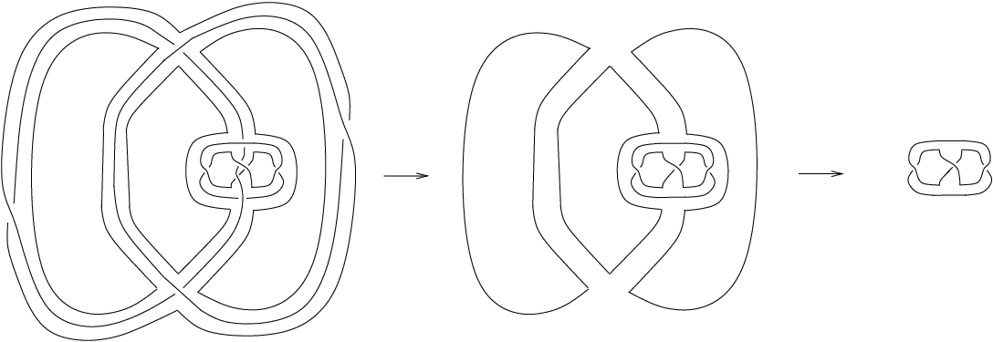
We study in this paper the Dehn fillings of the complement $N$ of the chain-link with 3 components in $S^{3}$ , shown in Fig. 1.

The hyperbolic structure of $N$ was first constructed by Thurston in his notes [27], and it was also noted there that the volume of $N$ is particularly small. The relevance of $N$ to 3-dimensional topology comes from the fact that filling $N$ one gets most of the hyperbolic manifolds known and most of the interesting non-hyperbolic fillings of cusped hyperbolic manifolds. For these reasons $N$ was called the “magic manifold” by Gordon and Wu [16, 13]. It appears as $M6_{1}^{3}$ in [6] and it is the hyperbolic manifold with $3$ cusps of smallest known volume and of smallest complexity [1]. (We refer here to the complexity defined by Matveev in [22], and we mean that $N$ has an ideal triangulation with $6$ tetrahedra, while all other hyperbolic manifolds with $3$ cusps need more than $6$ tetrahedra).

The main results of this paper, stated in Section 1, provide a complete classification (with prime and JSJ decomposition) of all non-hyperbolic Dehn fillings of $N$ , including partial ones. Quite some energy has been devoted in the literature to the understanding of exceptional slopes on hyperbolic manifolds, i.e. slopes giving non-hyperbolic fillings, but a complete description of the actual filled manifolds is seldom available. Our tables provide a complete description of the exceptional fillings for many hyperbolic manifolds with $1$ and $2$ cusps: for this reason we hope that our results will prove useful. We now list some consequences of this classification.

Surgery along knots in $S^{3}$

If the complement of a knot arises by filling two cusps of $N$ , its exceptional surgeries can be recovered from our tables. Every such knot has at least $4$ exceptional surgeries. In particular, we prove the following:

Theorem 1.

For every integer $n$ there are infinitely many hyperbolic knots in $S^{3}$ whose exceptional surgeries are $\{n,n+1,n+2,n+3\}$ , with $n$ and $n+3$ giving toroidal manifolds, and $n+1,n+2$ giving small Seifert manifolds.

Motegi and Song recently proved that for every $n$ there is a hyperbolic knot whose $n$ -surgery is small Seifert [23], and Teragaito proved the same result for toroidal surgeries [26]. Theorem 1 exhibits infinitely many examples for each $n$ . Other knots in $S^{3}$ with Seifert surgeries are also described in [7, 8, 21].

Seifert fillings

Following Gordon [13], let us say that a manifold is of type $D$ , $A$ , $S$ , or $T$ if it contains respectively an essential disc, annulus, sphere, or torus, and of type $S^{H}$ or $T^{H}$ if it contains a Heegaard sphere or torus. An exceptional filling of a hyperbolic $3$ -manifold is either of one of these types, or a small closed Seifert manifold, or a counterexample to the Geometrization Conjecture (which seems ruled out by Perelman). Detecting small Seifert fillings is the most difficult task, since these manifolds do not contain any small essential embedded surface (they only contain immersed essential tori).

Denoting by $\Delta$ the minimal geometric intersection between slopes on a torus, for $X_{0},X_{1}\in\{D,A,S,T,S^{H},T^{H}\}$ we define as in [13] the number $\Delta(X_{0},X_{1})$ as the maximum of $\Delta(\alpha_{0},\alpha_{1})$ over $M,\alpha_{0},\alpha_{1}$ , where $M$ is cusped hyperbolic, $\alpha_{0},\alpha_{1}$ are slopes on the same cusp of $M$ , and $M(\alpha_{i})$ is of type $X_{i}$ . All values of $\Delta(X_{0},X_{1})$ are known, except $\Delta(S,S^{H})$ and $\Delta(T,T^{H})$ , which are conjectured to be respectively $-\infty$ (this is the Cabling Conjecture) and $3$ . Our tables support both these conjectures.

Let us now say that a small Seifert manifold is of type $Z$ . As opposed to most values of $\Delta(X_{0},X_{1})$ for $X_{0},X_{1}\in\{D,S,A,T,S^{H},T^{H}\}$ , no value $\Delta(X,Z)$ seems to be known for $X\in\{S,T,S^{H},T^{H},Z\}$ . Our tables imply the following lower bounds:

	$S$	$T$	$S^{H}$	$T^{H}$	$Z$
$Z$	$2$	$7$	$1$	$2$	$6$

Infinitely many hyperbolic manifolds realize the following values:

	$S$	$T$	$S^{H}$	$T^{H}$	$Z$
$Z$	$2$	$5$	$1$	$2$	$4$

We have not found in the literature examples realizing greater values than those given by these tables.

Inequivalent knots with homeomorphic complements

The celebrated result of Gordon and Luecke [14] states that inequivalent knots in $S^{3}$ have non-homeomorphic complements. Here, two knots are equivalent when there is a self-homeomorphism of the ambient $3$ -manifold sending one to the other. Bleiler, Hodgson, and Weeks found two inequivalent hyperbolic knots in $L({\scriptstyle 49},{\scriptstyle 18})$ with homeomorphic complements (but the homeomorphism reverses the orientation). This example can be seen in our tables, and is still the only one known inside a closed manifold.

More examples arise in manifolds with boundary. There are infinitely many pairs of inequivalent hyperbolic knots with homeomorphic complements in the solid torus (their construction, due to Berge [2] and Gabai [12], led to the example in $L({\scriptstyle 49},{\scriptstyle 18})$ mentioned above) and in handlebodies of arbitrary genus [11]. We find in this paper some examples inside other manifolds:

Theorem 2.

The Whitehead sister link complement contains a pair of inequivalent hyperbolic knots with homeomorphic complements.

Theorem 3.

There exists a chiral Seifert manifold fibred over the disc with two exceptional fibres that contains a pair of inequivalent hyperbolic knots with orientation-preservingly homeomorphic complements.

The example provided by Theorem 2 is probably the first one discovered in a hyperbolic manifold. We note that the two inequivalent knots are geodesics of distinct length both having $N$ as a complement (but the homeomorphism between the complements reverses the orientation). The example provided by Theorem 3 is probably the first one of knots with orientation-preservingly homeomorphic complements in a chiral manifold (all other known examples are inside handlebodies).

Structure of the paper

The list of all non-hyperbolic Dehn fillings of $N$ is presented and discussed in Section 1, where we state several theorems and deduce from them some of the results announced in the present Introduction, and a few more. Section 2 contains the proofs of the classification theorems. The Appendix contains more tables (deduced from the lists in Section 1) showing the non-hyperbolic fillings of some notable classes of manifolds with one or two cusps. These further tables are used to prove the rest of the results stated above.

We warmly thank Jeff Weeks for very helpful suggestions on how to use SnapPea for the last step of the proof of Theorem 1.3.

1 Non-hyperbolic fillings of the chain-link complement

We state here the main results of the paper, namely Theorems 1.1, 1.2, and 1.3 which classify all non-hyperbolic fillings of the chain-link complement $N$ . We then use these results to prove the theorems stated in the Introduction.

1.1 Main results

To give our statements, we first make some conventions.

Homology bases

We fix the standard (meridian, longitude) homology basis on each component of $\partial N$ . Using it, we identify a slope $\alpha$ with a number in $\mathbb{Q}\cup\{\infty\}$ , and we denote by $N(\alpha)$ the Dehn filling of $N$ along $\alpha$ . Any two components of $\partial N$ can be interchanged by an automorphism which preserves the bases, so $N(\alpha)$ depends on $\alpha$ only. On each partial filling $N(\alpha)$ or $N(\alpha,\beta)$ we take the induced homology bases, and we note that the two components of $N(\alpha)$ are still symmetric.

Lens spaces

For simplicity we employ a more flexible notation for lens spaces than the usual one. We write $L({\scriptstyle 2},{\scriptstyle q})$ for $\mathbb{RP}^{3}$ , $L({\scriptstyle 1},{\scriptstyle q})$ for $S^{3}$ , $L({\scriptstyle 0},{\scriptstyle q})$ for $S^{2}\times S^{1}$ , and $L({\scriptstyle p},{\scriptstyle q})$ for $L({\scriptstyle|p|},{\scriptstyle q^{\prime}})$ with $q\equiv q^{\prime}\ (\textrm{mod }p)$ and $0<q^{\prime}<|p|$ , for any coprime $p,q$ .

Torus bundles

We denote by $T_{X}$ the torus bundle with monodromy $X\in{\rm GL}_{2}(\mathbb{Z})$ .

Seifert manifolds

If $F$ is a surface, $k\in\mathbb{N}$ , $b\in\mathbb{Z}$ and $\{(p_{i},q_{i})\}_{i=1}^{k}$ are coprime pairs with $|p_{i}|\geqslant 2$ , we define a Seifert manifold $\big(F,({\scriptstyle p_{1}},{\scriptstyle q_{1}}),\ldots,({\scriptstyle p_{k}},{\scriptstyle q_{k}}),b\big)$ as follows. Let $\Sigma$ be $F$ minus $k+1$ open discs and let $W$ be the orientable $S^{1}$ -bundle over $\Sigma$ . Give $W$ any orientation, pick a section $\sigma$ of $W$ , and choose positive homology bases $\{(\mu_{i},\lambda_{i})\}_{i=0}^{k}$ on the components of $\partial W$ arising from the punctures of $F$ , with $\mu_{i}\subset\partial\sigma$ and a fibre as $\lambda_{i}$ . Then $\big(F,({\scriptstyle p_{1}},{\scriptstyle q_{1}}),\ldots,({\scriptstyle p_{k}},{\scriptstyle q_{k}}),b\big)$ is the Dehn filling of $W$ along $p_{1}\mu_{1}+q_{1}\lambda_{1},\ldots,p_{k}\mu_{k}+q_{k}\lambda_{k},\mu_{0}+b\lambda_{0}$ .

We say the parameters are normalized if $p_{i}>q_{i}>0$ . In our statements we will allow parameters to be non-normalized only when they depend on some variable. Note that $b$ can be dismissed when $F$ has boundary and that our “filling parameters” $(p_{i},q_{i})$ are not the usual Seifert orbital parameters $(a_{i},b_{i})$ , which are computed as $a_{i}=|p_{i}|$ and $b_{i}\equiv q_{1}^{-1}\cdot{p_{i}}/{|p_{i}|}\ ({\rm mod}\ |p_{i}|)$ .

We denote by $D$ , $A$ , $S$ , $P$ , and $T$ respectively the disc, the annulus, the Möbius strip, the pair of pants, and the torus.

Graph manifolds

If $F$ is an orientable surface with $h\geqslant 1$ boundary components and $\Sigma$ is $F$ minus $k$ discs, we proceed as above to construct homology bases $\{(\mu_{i},\lambda_{i})\}_{i=1}^{h+k}$ on $\partial(\Sigma\times S^{1})$ , with the extra requirement that the $\mu_{i}$ ’s should be oriented as components of $\partial\Sigma$ . For coprime pairs $\{(p_{i},q_{i})\}_{i=1}^{k}$ with $|p_{i}|\geqslant 2$ we then get a Seifert manifold $\big(F,({\scriptstyle p_{1}},{\scriptstyle q_{1}}),\ldots,({\scriptstyle p_{k}},{\scriptstyle q_{k}})\big)$ with fixed homology bases on its $h$ boundary components. If $M,M^{\prime}$ are Seifert manifolds with boundary and orientable base surfaces, and $X\in{\rm GL}_{2}(\mathbb{Z})$ , we can then define without ambiguity $M\cup_{X}M^{\prime}$ to mean $M\cup_{f}M^{\prime}$ with $f:T\to T^{\prime}$ , where $T$ and $T^{\prime}$ are arbitrary boundary tori of $M$ and $M^{\prime}$ , respectively, and $f$ acts on homology as $X$ with respect to the fixed bases. Similarly we can define $M\big/_{X}$ when $M$ has at least 2 components.

We are now ready to give our statements, which correspond to the filling of 1, 2, or all 3 components of $\partial N$ , respectively. Throughout this paper ‘hyperbolic’ means ‘finite-volume complete hyperbolic,’ and the symbol $N$ is only used to denote the complement of the 3-components chain-link in $S^{3}$ , shown in Fig. 1.

Theorem 1.1.

$N(\alpha)$ is hyperbolic unless $\alpha\in\{\infty,-3,-2,-1,0\}$ , and:

•

$N(\infty)=T\times I$ ;
•

$N(-3)=\big(A,({\scriptstyle 2},{\scriptstyle 1})\big)\bigcup\nolimits_{{\tiny{\left(\begin{array}[]{@{}c@{\ }c@{}}0&1\\ 1&0\\ \end{array}\right)}}\phantom{\Big|}\!\!}\big(A,({\scriptstyle 2},{\scriptstyle 1})\big)$ ;
•

$N(-2)=\big(P,({\scriptstyle 3},{\scriptstyle 1})\big)$ ;
•

$N(-1)=\big(P,({\scriptstyle 2},{\scriptstyle 1})\big)$ ;
•

$N(0)=\big(D,({\scriptstyle 2},{\scriptstyle 1}),({\scriptstyle 3},{\scriptstyle 1})\big)\bigcup\nolimits_{{\tiny{\left(\begin{array}[]{@{}c@{\ }c@{}}1&1\\ -1&0\\ \end{array}\right)}}\phantom{\Big|}\!\!}\big(P\times S^{1}\big)$ .

Theorem 1.2.

$M=N(p/q,r/s)$ is hyperbolic except if one of the following occurs up to permutation:

•

$p/q\in\{\infty,-3,-2,-1,0\}$ ;
•

$(p/q,r/s)\in\{(1,1),(-4,-1/2),(-3/2,-5/2)\}$ .

In all cases $M$ is as shown in Table 1, where $n$ stands for a generic integer and $r/s\neq\infty$ unless $p/q=\infty$ .

$p/q$	$r/s$	$M$
$\infty$	any	$D\times S^{1}$
$-3$	$-1$	$\mathbb{RP}^{3}\#(D\times S^{1})$
	$-2$	$D\times S^{1}$
	$-3$	$\big(S,({\scriptstyle 2},{\scriptstyle 1})\big)$
	$-1+\frac{1}{n},\neq-2$	$\big(D,({\scriptstyle 2},{\scriptstyle 1}),({\scriptstyle 2n+1},{\scriptstyle 2})\big)$
	$\neq-1,\neq-1+\frac{1}{n}$	$\big(D,({\scriptstyle 2},{\scriptstyle 1}),({\scriptstyle r+s},{\scriptstyle s})\big)\bigcup\nolimits_{{\tiny{\left(\begin{array}[]{@{}c@{\ }c@{}}0&1\\ 1&0\\ \end{array}\right)}}\phantom{\Big\|}\!\!}\big(A,({\scriptstyle 2},{\scriptstyle 1})\big)$
$-2$	$-2$	$L({\scriptstyle 3},{\scriptstyle 1})\#(D\times S^{1})$
	$-2+\frac{1}{n}$	$D\times S^{1}$
	$\neq-2,\neq-2+\frac{1}{n}$	$\big(D,({\scriptstyle 3},{\scriptstyle 1}),({\scriptstyle r+2s},{\scriptstyle s})\big)$
$-1$	$-3$	$\mathbb{RP}^{3}\#(D\times S^{1})$
	$-3+\frac{1}{n}$	$D\times S^{1}$
	$\neq-3,\neq-3+\frac{1}{n}$	$\big(D,({\scriptstyle 2},{\scriptstyle 1}),({\scriptstyle r+3s},{\scriptstyle s})\big)$
$0$	$\in\mathbb{Z}$	$\big(D,({\scriptstyle 2},{\scriptstyle 1}),({\scriptstyle 3},{\scriptstyle 1})\big)$
	$\not\in\mathbb{Z}$	$\big(D,({\scriptstyle 2},{\scriptstyle 1}),({\scriptstyle 3},{\scriptstyle 1})\big)\bigcup\nolimits_{{\tiny{\left(\begin{array}[]{@{}c@{\ }c@{}}1&1\\ -1&0\\ \end{array}\right)}}\phantom{\Big\|}\!\!}\big(A,({\scriptstyle s},{\scriptstyle r})\big)$
$1$	$1$	$\big(P\times S^{1}\big)\big/_{{\tiny{\left(\begin{array}[]{@{}c@{\ }c@{}}0&1\\ 1&0\\ \end{array}\right)}}\phantom{\Big\|}\!\!}$
$-\frac{3}{2}$	$-\frac{5}{2}$	$\big(D,({\scriptstyle 2},{\scriptstyle 1}),({\scriptstyle 3},{\scriptstyle 1})\big)\bigcup\nolimits_{{\tiny{\left(\begin{array}[]{@{}c@{\ }c@{}}1&1\\ -1&0\\ \end{array}\right)}}\phantom{\Big\|}\!\!}\big(A,({\scriptstyle 2},{\scriptstyle 1})\big)$
$-4$	$-\frac{1}{2}$	$\big(D,({\scriptstyle 2},{\scriptstyle 1}),({\scriptstyle 3},{\scriptstyle 1})\big)\bigcup\nolimits_{{\tiny{\left(\begin{array}[]{@{}c@{\ }c@{}}1&1\\ -1&0\\ \end{array}\right)}}\phantom{\Big\|}\!\!}\big(A,({\scriptstyle 2},{\scriptstyle 1})\big)$

Table 1: Classification of non-hyperbolic fillings of

N

with 1 boundary component

Theorem 1.3.

$M=N(p/q,r/s,t/u)$ is hyperbolic except if one the following occurs up to permutation:

•

$p/q=\infty$ , in which case $M=L({\scriptstyle tr-us},{\scriptstyle tr^{\prime}-us^{\prime}})$ , where $r^{\prime},s^{\prime}\in\mathbb{Z}$ are such that $rs^{\prime}-sr^{\prime}=\pm 1$ ;
•

$p/q\in\{-3,-2,-1,0\}$ , in which case $M$ is as described in Table 2 (with $n$ and $m$ standing for generic integers);
•

$(p/q,r/s)\in\{(1,1),(-4,-1/2),(-3/2,-5/2)\}$ , in which case $M$ is as described in Table 3;
•

$(p/q,r/s,t/u)$ is one of the 14 triples listed in Table 4, together with a description of the corresponding $M$ .

$p/q$	$r/s$	$t/u$	$M$
$-3$	$1$ or $-\frac{5}{3}$	$r/s$	$(K,1)\phantom{\Big\|}$
	$-1$	any	$\mathbb{RP}^{3}\#L({\scriptstyle t+3u},{\scriptstyle u})\phantom{\Big\|}$
	$-2$	any	$L({\scriptstyle 5t+7u},{\scriptstyle 2t+3u})\phantom{\Big\|}$
	$-1+\frac{1}{n}\phantom{\Big\|}$	$-1+\frac{1}{m}$	$L({\scriptstyle(2n+1)(2m+1)-4},{\scriptstyle(2n+1)m-2})$
	$\neq-2$	$\neq-1,\ \neq-1+\frac{1}{m}\phantom{\Big\|}\!\!$	$\big(S^{2},({\scriptstyle 2},{\scriptstyle 1}),({\scriptstyle 2n+1},{\scriptstyle-2}),({\scriptstyle t+u},{\scriptstyle u})\big)$
	$-3$	$\neq-1,\ \neq-1+\frac{1}{m}\phantom{\Big\|}\!\!$	$\big(\mathbb{RP}^{2},({\scriptstyle 2},{\scriptstyle 1}),({\scriptstyle t+u},{\scriptstyle u})\big)$
	$\begin{array}[]{c}\neq-1,\ \neq-3\\ \neq-1+\frac{1}{n}\end{array}$	$\begin{array}[]{c}\neq-1,\ \neq-3\\ \neq-1+\frac{1}{m}\\ \neq\frac{r}{s}\ {\rm if}\ \frac{r}{s}\in\{1,-\frac{5}{3}\}\end{array}$	$\begin{array}[]{l}\big(D,({\scriptstyle 2},{\scriptstyle 1}),({\scriptstyle r+s},{\scriptstyle s})\big)\bigcup\nolimits_{\tiny{\left(\begin{array}[]{@{}c@{\ }c@{}}0&1\\ 1&0\\ \end{array}\right)}}\\ \big(D,({\scriptstyle 2},{\scriptstyle 1}),({\scriptstyle t+u},{\scriptstyle u})\big)\end{array}$
$-2$	$-2$	any	$L({\scriptstyle 3},{\scriptstyle 1})\#L({\scriptstyle t+2u},{\scriptstyle u})\phantom{\Big\|}$
	$-2+\frac{1}{n}$	any	$L({\scriptstyle 3n(t+2u)-2t-u},{\scriptstyle n(t+2u)-t-u})\phantom{\Big\|}$
	$\begin{array}[]{c}\neq-2\\ \neq-2+\frac{1}{n}\end{array}$	$\begin{array}[]{c}\neq-2\\ \neq-2+\frac{1}{m}\end{array}$	$\big(S^{2},({\scriptstyle 3},{\scriptstyle 2}),({\scriptstyle r+2s},{\scriptstyle-s}),({\scriptstyle t+2u},{\scriptstyle-u})\big)$
$-1$	$-3$	any	$\mathbb{RP}^{3}\#L({\scriptstyle t+3u},{\scriptstyle u})\phantom{\Big\|}$
	$-3+\frac{1}{n}$	any	$L({\scriptstyle 2n(t+3u)-t-u},{\scriptstyle n(t+3u)+u})\phantom{\Big\|}$
	$\begin{array}[]{c}\neq-3\\ \neq-3+\frac{1}{n}\end{array}$	$\begin{array}[]{c}\neq-3\\ \neq-3+\frac{1}{m}\end{array}$	$\big(S^{2},({\scriptstyle 2},{\scriptstyle 1}),({\scriptstyle r+3s},{\scriptstyle-s}),({\scriptstyle t+3u},{\scriptstyle-u})\big)$
$0$	$n$	$-4-n$	$\mathbb{RP}^{3}\#L({\scriptstyle 3},{\scriptstyle 1})\phantom{\Big\|}$
		$-4-n+\frac{1}{m}$	$L({\scriptstyle 6m-1},{\scriptstyle 2m-1})\phantom{\Big\|}$
		$\begin{array}[]{c}\neq-4-n\\ \neq-4-n+\frac{1}{m}\end{array}$	$\big(S^{2},({\scriptstyle 2},{\scriptstyle-1}),({\scriptstyle 3},{\scriptstyle 1}),({\scriptstyle t+(n+4)u},{\scriptstyle u})\big)$
	$\frac{1}{2}+n$	$-\frac{9}{2}-n$	$\big(\mathbb{RP}^{2},({\scriptstyle 2},{\scriptstyle 1}),({\scriptstyle 3},{\scriptstyle 1}),-1\big)\phantom{\Big\|}$
	$\not\in\mathbb{Z}$	$\begin{array}[]{c}\not\in\mathbb{Z}\\ \neq-\frac{r}{s}-4\ {\rm if}\ \|s\|=2\end{array}$	$\begin{array}[]{l}\big(D,({\scriptstyle s},{\scriptstyle r+2s}),({\scriptstyle u},{\scriptstyle t+2u})\big)\bigcup\nolimits_{\tiny{\left(\begin{array}[]{@{}c@{\ }c@{}}0&1\\ -1&-1\\ \end{array}\right)}}\\ \big(D,({\scriptstyle 2},{\scriptstyle 1}),({\scriptstyle 3},{\scriptstyle 1})\big)\end{array}$

Table 2: Classification of closed non-hyperbolic fillings of

N

$p/q$	$r/s$	$t/u$	$M$
$1$	$1$	$n$	$T_{{\tiny{\left(\begin{array}[]{@{}c@{\ }c@{}}n+1&1\\ -1&0\\ \end{array}\right)}}\phantom{\Big\|}}\phantom{\Big\|}$
		$\not\in\mathbb{Z}$	$\big(A,({\scriptstyle u},{\scriptstyle t+u})\big)\big/_{{\tiny{\left(\begin{array}[]{@{}c@{\ }c@{}}0&1\\ 1&0\\ \end{array}\right)}}\phantom{\Big\|}}\phantom{\Big\|}$
$-3/2$	$-5/2$	$-2$	$\mathbb{RP}^{3}\phantom{\Big\|}$
		$-1$	$L({\scriptstyle 13},{\scriptstyle 5})\phantom{\Big\|}$
		$0$	$\big(\mathbb{RP}^{2},({\scriptstyle 2},{\scriptstyle 1}),({\scriptstyle 3},{\scriptstyle 1}),-1\big)\phantom{\Big\|}$
		$\begin{array}[]{c}-2+\frac{1}{n}\\ \neq-1\end{array}$	$\big(S^{2},({\scriptstyle 2},{\scriptstyle 1}),({\scriptstyle 3},{\scriptstyle-1}),({\scriptstyle 2n-1},{\scriptstyle 2})\big)$
		$\begin{array}[]{c}\neq 0\\ \neq-2\\ \neq-2+\frac{1}{n}\end{array}$	$\begin{array}[]{l}\big(D,({\scriptstyle 2},{\scriptstyle 1}),({\scriptstyle 3},{\scriptstyle 1})\big)\bigcup\nolimits_{\tiny{\left(\begin{array}[]{@{}c@{\ }c@{}}1&1\\ 0&-1\\ \end{array}\right)}}\\ \big(D,({\scriptstyle 2},{\scriptstyle 1}),({\scriptstyle t+2u},{\scriptstyle u})\big)\end{array}$
$-4$	$-1/2$	$-1$	$L({\scriptstyle 11},{\scriptstyle 3})\phantom{\Big\|}$
		$-\frac{1}{2}$	$\big(\mathbb{RP}^{2},({\scriptstyle 2},{\scriptstyle 1}),({\scriptstyle 3},{\scriptstyle 1}),-1\big)\phantom{\Big\|}$
		$0$	$L({\scriptstyle 13},{\scriptstyle 5})\phantom{\Big\|}$
		$\begin{array}[]{c}n\\ \neq-1\\ \neq 0\end{array}$	$\big(S^{2},({\scriptstyle 2},{\scriptstyle 1}),({\scriptstyle 3},{\scriptstyle-1}),({\scriptstyle 2n+1},{\scriptstyle 2})\big)$
		$\not\in\mathbb{Z}\cup\{-\frac{1}{2}\}$	$\begin{array}[]{l}\big(D,({\scriptstyle 2},{\scriptstyle 1}),({\scriptstyle 3},{\scriptstyle 1})\big)\bigcup\nolimits_{\tiny{\left(\begin{array}[]{@{}c@{\ }c@{}}1&1\\ 1&0\\ \end{array}\right)}}\\ \big(D,({\scriptstyle 2},{\scriptstyle 1}),({\scriptstyle u},{\scriptstyle t})\big)\end{array}$

Table 3: Classification of closed non-hyperbolic fillings of

N

(continued)

$p/q$	$r/s$	$t/u$	$M$
$-5$	$-5$	$-1/2$	$\big(A,({\scriptstyle 2},{\scriptstyle 1})\big)\big/_{{\tiny{\left(\begin{array}[]{@{}c@{\ }c@{}}0&1\\ 1&0\\ \end{array}\right)}}\phantom{\Big\|}}\phantom{\Big\|}$
$-4$	$-4$	$-2/3$	$\big(A,({\scriptstyle 2},{\scriptstyle 1})\big)\big/_{{\tiny{\left(\begin{array}[]{@{}c@{\ }c@{}}1&1\\ 1&0\\ \end{array}\right)}}\phantom{\Big\|}}\phantom{\Big\|}$
$-4$	$-3/2$	$-3/2$	$T_{{\tiny{\left(\begin{array}[]{@{}c@{\ }c@{}}-3&1\\ -1&0\\ \end{array}\right)}}\phantom{\Big\|}}\phantom{\Big\|}$
$-4$	$-1/3$	$1$	$\big(D,({\scriptstyle 2},{\scriptstyle 1}),({\scriptstyle 2},{\scriptstyle 1})\big)\bigcup\nolimits_{{\tiny{\left(\begin{array}[]{@{}c@{\ }c@{}}0&1\\ -1&-1\\ \end{array}\right)}}\phantom{\Big\|}\!\!}\big(D,({\scriptstyle 2},{\scriptstyle 1}),({\scriptstyle 3},{\scriptstyle 1})\big)\phantom{\Big\|}$
$-8/3$	$-3/2$	$-3/2$	$\big(D,({\scriptstyle 2},{\scriptstyle 1}),({\scriptstyle 2},{\scriptstyle 1})\big)\bigcup\nolimits_{{\tiny{\left(\begin{array}[]{@{}c@{\ }c@{}}0&1\\ -1&-1\\ \end{array}\right)}}\phantom{\Big\|}\!\!}\big(D,({\scriptstyle 2},{\scriptstyle 1}),({\scriptstyle 3},{\scriptstyle 1})\big)\phantom{\Big\|}$
$-5/2$	$-5/2$	$-4/3$	$\big(A,({\scriptstyle 2},{\scriptstyle 1})\big)\big/_{{\tiny{\left(\begin{array}[]{@{}c@{\ }c@{}}2&1\\ 1&0\\ \end{array}\right)}}\phantom{\Big\|}}\phantom{\Big\|}$
$-5/2$	$-5/3$	$-5/3$	$\big(D,({\scriptstyle 2},{\scriptstyle 1}),({\scriptstyle 2},{\scriptstyle 1})\big)\bigcup\nolimits_{{\tiny{\left(\begin{array}[]{@{}c@{\ }c@{}}-1&1\\ 0&-1\\ \end{array}\right)}}\phantom{\Big\|}\!\!}\big(D,({\scriptstyle 2},{\scriptstyle 1}),({\scriptstyle 3},{\scriptstyle 1})\big)\phantom{\Big\|}$
$-7/3$	$-7/3$	$-3/2$	$\big(A,({\scriptstyle 2},{\scriptstyle 1})\big)\big/_{{\tiny{\left(\begin{array}[]{@{}c@{\ }c@{}}1&1\\ 1&0\\ \end{array}\right)}}\phantom{\Big\|}}\phantom{\Big\|}$
$1$	$2$	$2$	$\big(S^{2},({\scriptstyle 2},{\scriptstyle 1}),({\scriptstyle 3},{\scriptstyle 1}),({\scriptstyle 7},{\scriptstyle 1}),-1\big)\phantom{\Big\|}$
$1$	$2$	$3$	$\big(S^{2},({\scriptstyle 2},{\scriptstyle 1}),({\scriptstyle 4},{\scriptstyle 1}),({\scriptstyle 5},{\scriptstyle 1}),-1\big)\phantom{\Big\|}$
$1$	$2$	$4$	$\big(S^{2},({\scriptstyle 3},{\scriptstyle 1}),({\scriptstyle 3},{\scriptstyle 1}),({\scriptstyle 4},{\scriptstyle 1}),-1\big)\phantom{\Big\|}$
$1$	$2$	$5$	$\big(D,({\scriptstyle 2},{\scriptstyle 1}),({\scriptstyle 2},{\scriptstyle 1})\big)\bigcup\nolimits_{{\tiny{\left(\begin{array}[]{@{}c@{\ }c@{}}0&1\\ 1&0\\ \end{array}\right)}}\phantom{\Big\|}\!\!}\big(D,({\scriptstyle 2},{\scriptstyle 1}),({\scriptstyle 3},{\scriptstyle 1})\big)\phantom{\Big\|}$
$1$	$3$	$3$	$\big(D,({\scriptstyle 2},{\scriptstyle 1}),({\scriptstyle 2},{\scriptstyle 1})\big)\bigcup\nolimits_{{\tiny{\left(\begin{array}[]{@{}c@{\ }c@{}}1&2\\ 0&-1\\ \end{array}\right)}}\phantom{\Big\|}\!\!}\big(D,({\scriptstyle 2},{\scriptstyle 1}),({\scriptstyle 3},{\scriptstyle 1})\big)\phantom{\Big\|}$
$2$	$2$	$2$	$\big(D,({\scriptstyle 2},{\scriptstyle 1}),({\scriptstyle 2},{\scriptstyle 1})\big)\bigcup\nolimits_{{\tiny{\left(\begin{array}[]{@{}c@{\ }c@{}}2&3\\ -1&-2\\ \end{array}\right)}}\phantom{\Big\|}\!\!}\big(D,({\scriptstyle 2},{\scriptstyle 1}),({\scriptstyle 3},{\scriptstyle 1})\big)\phantom{\Big\|}$

Table 4: Classification of closed non-hyperbolic fillings of

N

(continued)

The next remark is important to understand the statement of Theorem 1.3.

Remark 1.4.

We have compiled Tables 2 to 4 trying to keep them concise but easily usable. In particular:

•

we have always excluded the case where one of the filling coefficients is $\infty$ , because the first point of Theorem 1.3 is already sufficient in this case to determine which lens space the result is;
•

whenever a certain value $p/q\in\{-3,-2,-1,0\}$ is chosen, the corresponding set of lines in Table 2 contains a complete classification of the resulting $M$ , but one may have to permute $r/s$ and $t/u$ to get the result;
•

the tables always provide the decomposition of $M$ into prime connected summands and the JSJ decomposition of these summands, except when a connected sum involves a lens space and the parameters are such that the lens space is $S^{3}$ ;
•

the triples listed in Table 4 do not appear in Tables 2 and 3;
•

there is some overlapping between the cases covered in Tables 2 and 3. The recognition of $M$ is of course coherent (note for instance that $N(1,1,n)=T_{\tiny\left(\begin{array}[]{@{}c@{\ }c@{}}n+1&1\\ -1&0\\ \end{array}\right)}$ is also a Seifert manifold for $n\in\{-3,-2,-1,0\}$ , see Lemma 2.1);
•

in Table 3 the elements of each triple are arranged in increasing order, and the triples themselves are arranged in a lexicographically increasing order.

Sketch of the proofs

The proof of Theorems 1.1 to 1.3 goes as follows: we first prove Theorem 1.1 using spines. Actually, we prove a more refined version of it, in which we determine the image in $N(\alpha)$ of the bases of the non-filled boundary tori. Using spines, we also recognize $N(1,1),$ $N(2,2,2),$ and $N(1,3,3)$ . We then use Proposition 1.5 below (discussed in Section 2) to recognize all the other fillings listed in Tables 1 to 4. Next, we use the Gromov-Thurston $2\pi$ theorem to show that if $M$ is a filling of $N$ , but not one of those already recognized to be non-hyperbolic, then $M$ admits a complete metric with negative sectional curvature. An application of the orbifold theorem [4] then implies that $M$ is actually hyperbolic. This is because our chain-link complement $N$ admits an orientation-preserving order- $2$ involution, given by a rotation of angle $\pi$ around a horizontal circle in Fig. 1. Its effect on the homology of each cusp is given by multiplication by $-1$ , therefore the involution extends to every Dehn filling of $N$ . The orbifold theorem then guarantees that each filling of $N$ satisfies the geometrization conjecture.

Proposition 1.5.

$N(-3/2)=N(-4)$ and the following holds for all $\alpha,\beta\in\mathbb{Q}\cup\{\infty\}$ :

$\displaystyle N\left(-\frac{3}{2},\alpha,\beta\right)$	$\displaystyle=$	$\displaystyle N\left(-4,-\frac{\alpha+1}{\alpha+2},-\beta-3\right)$	(1)
$\displaystyle N\left(-\frac{5}{2},\alpha,\beta\right)$	$\displaystyle=$	$\displaystyle N\left(-\frac{5}{2},-\frac{\alpha+3}{\alpha+2},-\frac{2\beta+3}{\beta+1}\right)$	(2)
$\displaystyle N\left(-\frac{3}{2},\alpha,\beta\right)$	$\displaystyle=$	$\displaystyle N\left(-\frac{3}{2},-\frac{2\alpha+5}{\alpha+2},-\frac{2\beta+5}{\beta+2}\right)$	(3)
$\displaystyle N\left(-\frac{1}{2},\alpha,\beta\right)$	$\displaystyle=$	$\displaystyle N\left(-\frac{1}{2},-\alpha-4,-\beta-4\right)$	(4)
$\displaystyle N\left(1,2,\alpha\right)$	$\displaystyle=$	$\displaystyle N\left(1,2,-\alpha+2\right)$	(5)
$\displaystyle N\left(1,-4,\alpha\right)$	$\displaystyle=$	$\displaystyle N\left(1,-4,\frac{1}{\alpha}\right)$	(6)

Relations (2) to (6) are induced by automorphisms of $N(-5/2)$ , $N(-3/2)$ , $N(-1/2)$ , $N(1,2)$ , and $N(1,-4)$ , respectively. Moreover (2) has order $3$ , while (3)-(6) have order $2$ .

We note that $N$ and the manifolds involved in Proposition 1.5 are well-known hyperbolic ones. Using SnapPea one sees that $N$ is the manifold called the “magic” one in [16] and listed as $M6_{1}^{3}$ in [6].

Some important fillings of $N$ are link complements in the 3-sphere: $N(-4)=N(-3/2)$ of the Whitehead sister link, $N(-5/2)$ of the Berge link, $N(-1/2)$ of the $3/10$ -bridge link, $N(1)$ of the Whitehead link. In addition $N(1,2)$ is the figure-8 knot complement and $N(1,-4)$ is the figure-8 knot sister. See the Appendix for more details on these manifolds and their fillings. We show the slopes involved in these fillings in Fig. 2 where we arrange them on $\partial\mathbb{H}^{2}=\mathbb{Q}\cup\{\infty\}$ using the disc model of $\mathbb{H}^{2}$ , and we connect by lines slopes having distance $1$ , thus showing a partial picture of the so-called Farey tessellation.

1.2 Some consequences

We illustrate here some facts that can be deduced from our main statements.

Seifert fillings

We begin by proving Theorem 1 as a consequence of the following:

Proposition 1.6.

For every integer $k\neq 0$ , among the manifolds of the form $N\left(1+\frac{1}{h},\frac{kh+1}{k(h+1)+1}\right)$ , with $h\in\mathbb{Z}$ , there are infinitely many distinct hyperbolic ones whose exceptional slopes are precisely $\infty,-3,-2,-1,0$ . Moreover

•

The $\infty$ -filling is $S^{3}$ ;
•

The $(-3)$ -filling and the $0$ -filling are toroidal;
•

The $(-2)$ -filling and the $(-1)$ -filling are small Seifert manifolds with first homology respectively $\mathbb{Z}/_{(k+3)\mathbb{Z}}$ and $\mathbb{Z}/_{(k+2)\mathbb{Z}}$ .

Proof.

A manifold $M$ as described is hyperbolic by Theorem 1.2, except for finitely many values of $h$ . Moreover as $h$ goes to $\infty$ the volume of $M$ tends to the volume of $N$ from below, so there are infinitely many different $M$ ’s. For the other assertions, setting $r/s=(h+1)/h$ and $t/u=(kh+1)/(k(h+1)+1)$ , we have

tr-us=\det\left(\begin{array}[]{@{}c@{\ }c@{}}r&u\\ s&t\\ \end{array}\right)=\det\left(\begin{array}[]{@{}c@{\ }c@{}}h+1&1+k(h+1)\\ h&1+kh\\ \end{array}\right)=\det\left(\begin{array}[]{@{}c@{\ }c@{}}h+1&1\\ h&1\\ \end{array}\right)=1

which implies (by the first assertion of Theorem 1.3) that $M(\infty)=S^{3}$ . As $h$ tends to $\infty$ (while $k$ stays fixed) both $r/s$ and $t/u$ tend to $1$ , and it easily follows from Table 2 that only finitely many values of $h$ can yield manifolds of non-generic type for $M(-3),M(-2),M(-1)$ , and $M(0)$ . Then for infinitely many $h$ ’s the topology of the fillings is as required. We are left to prove the assertion concerning homology.

It is easy to see that the number $\nu=|q_{1}p_{2}p_{3}+q_{2}p_{3}p_{1}+q_{3}p_{1}p_{2}|$ equals the cardinality of $H_{1}\big(S^{2},(p_{1},q_{1}),(p_{2},q_{2}),(p_{3},q_{3})\big)$ except when $\nu=0$ , in which case the group is infinite. When the Seifert manifold is obtained from surgery on a knot in $S^{3}$ , its first homology group must be $\mathbb{Z}/_{\nu\mathbb{Z}}$ . Therefore:

$\displaystyle H_{1}\big(M(-2)\big)$	$\displaystyle=$	$\displaystyle H_{1}\big(S^{2},(3,2),(r+2s,-s),(t+2u,-u)\big)$
	$\displaystyle=$	$\displaystyle\mathbb{Z}/_{(2(r+2s)(t+2u)-3s(t+2u)-3u(r+2s))\mathbb{Z}}$
	$\displaystyle=$	$\displaystyle\mathbb{Z}/_{(2rt+ru+st-4su)\mathbb{Z}}=\mathbb{Z}/_{((r-s)(u-t)+3(rt-su))\mathbb{Z}}=\mathbb{Z}/_{(k+3)\mathbb{Z}}$

and similarly $H_{1}\big(M(-1)\big)=\mathbb{Z}_{(k+2)\mathbb{Z}}$ . ∎

Proof of Theorem 1. Fix $n$ , assume first $n\neq-4$ , and apply Proposition 1.6 with $k=-n-4$ . Each of the manifolds given by the proposition is the complement of a knot having 4 consecutive integer exceptional slopes, say $a,a+1,a+2,a+3$ . Since the first homology of a $b$ -surgery on a knot is $\mathbb{Z}/_{b\mathbb{Z}}$ , we deduce that

\mathbb{Z}/_{(a+1)\mathbb{Z}}=\mathbb{Z}/_{(k+3)\mathbb{Z}},\qquad\mathbb{Z}/_{(a+2)\mathbb{Z}}=\mathbb{Z}/_{(k+2)\mathbb{Z}}.

Now $k+3=-(n+1)$ and $k+2=-(n+2)$ , whence $a+1=\pm(n+1)$ and $a+2=\pm(n+2)$ , whose only solution is $a=n$ . This implies that we have infinitely many knots with exceptional slopes $n,n+1,n+2,n+3$ as required. For $n=-4$ it is sufficient to take the knots for $n=1$ and consider their mirror images. $\square$

Knots with homeomorphic complements

We discuss here Theorems 2 and 3. As usual, we translate them into a statement about Dehn fillings: two inequivalent knots in $M$ having the same $M^{\prime}$ as their complement correspond to inequivalent slopes in $\partial M^{\prime}$ both giving $M$ via Dehn filling. Two slopes are equivalent if there is an automorphism of $M^{\prime}$ sending one to the other.

We also recall some other definitions from [5]. Two slopes $\alpha$ and $\beta$ such that $M^{\prime}(\alpha)$ is homeomorphic to $M^{\prime}(\beta)$ are called cosmetic. Taking on $M^{\prime}(\alpha)$ and $M^{\prime}(\beta)$ an orientation that extends one and the same orientation of $M^{\prime}$ , we say that $\alpha$ and $\beta$ are truly cosmetic if there is an orientation-preserving homeomorphism from $M^{\prime}(\alpha)$ to $M^{\prime}(\beta)$ , and reflectively cosmetic if there is an orientation-reversing one (both possibilities can hold).

The only known $1$ -cusped hyperbolic $M$ with a pair of inequivalent cosmetic slopes was found in [5] and it is $M=N(-5/2,-2/5)$ which admits the cosmetic pair of slopes $-2,-1$ giving $L({\scriptstyle 49},{\scriptstyle 18})$ , as one sees from Table 2 or Table 13 in the Appendix. The two slopes are not truly cosmetic. In fact, it is conjectured [5, 18] that inequivalent slopes on a $1$ -cusped $M$ are never truly cosmetic.

Cosmetic phenomena seem to be more frequent on manifolds with more cusps. All the $2$ -cusped $M$ ’s with distinct slopes $\alpha,\beta$ on a torus $T\subset\partial M$ such that $M(\alpha)=M(\beta)$ is a solid torus are described by Berge and Gabai in [2, 12]. Infinitely many such pairs of slopes are inequivalent. This also follows from the next result, proved in Subsection A.1 of the Appendix, which implies Theorem 2 and 3 too.

Theorem 1.7.

Let $M$ be $N$ or a hyperbolic $N(\gamma)$ , and let $\alpha,\beta$ be a cosmetic pair of inequivalent slopes on $M$ . Then $M,\alpha,\beta$ are as in Table 5.

$M$	$\alpha$	$\beta$	$M(\alpha)$	truly	reflectively
$N$	$-4$	$-3/2$	Whitehead sister	no	yes
$\begin{array}[]{c}N(-3+1/n)\\ n\in\mathbb{Z}\setminus\{0,\pm 1,2\}\end{array}$	$\infty$	$-1$	$D\times S^{1}$	yes	yes
$\begin{array}[]{c}N(-2+1/n)\\ n\in\mathbb{Z}\setminus\{0,\pm 1,\pm 2\}\end{array}$	$\infty$	$-2$	$D\times S^{1}$	yes	yes
$N(-12/5)$	$-2$	$-1$	$\big(D,({\scriptstyle 2},{\scriptstyle 1}),({\scriptstyle 3},{\scriptstyle 1})\big)$	yes	no
$N(-6)$	$-1$	$0$	$\big(D,({\scriptstyle 2},{\scriptstyle 1}),({\scriptstyle 3},{\scriptstyle 1})\big)$	no	yes
$N(-4/3)$	$-3$	$-1$	$\big(D,({\scriptstyle 2},{\scriptstyle 1}),({\scriptstyle 5},{\scriptstyle 2})\big)$	no	yes

Table 5: Cosmetic slopes on

N

and

N(\gamma)

Using SnapPea, one sees that the two cosmetic knots in the Whitehead link sister corresponding to the first line of Table 5 are the two shortest geodesics, with lengths $0.96242\ldots$ and $1.06128\ldots$ .

Non-hyperbolic closed fillings

The following result is easily proved as a consequence of Theorem 1.3 and Lemma 2.1:

Corollary 1.8.

The set of all non-hyperbolic closed manifolds obtained by Dehn surgery on the chain-link consists of:

•

$S^{3}$ , $S^{2}\times S^{1}$ , $L({\scriptstyle p},{\scriptstyle q})$ ,
•

$\mathbb{RP}^{3}\#L({\scriptstyle p},{\scriptstyle q})$ , $L({\scriptstyle 3},{\scriptstyle 1})\#L({\scriptstyle p},{\scriptstyle q})$ , $\mathbb{RP}^{3}\#(S^{2}\times S^{1})$ , $L({\scriptstyle 3},{\scriptstyle 1})\#(S^{2}\times S^{1})$ ,
•

$\big(S^{2},({\scriptstyle 2},{\scriptstyle 1}),({\scriptstyle p},{\scriptstyle q}),({\scriptstyle r},{\scriptstyle s}),b\big),\big(S^{2},({\scriptstyle 3},{\scriptstyle 1}),({\scriptstyle p},{\scriptstyle q}),({\scriptstyle r},{\scriptstyle s}),b\big),\big(\mathbb{RP}^{2},({\scriptstyle 2},{\scriptstyle 1}),({\scriptstyle p},{\scriptstyle q}),b\big)$ ,
•

$\big(D,({\scriptstyle 2},{\scriptstyle 1}),({\scriptstyle p},{\scriptstyle q})\big)\bigcup_{X}\big(D,({\scriptstyle 2},{\scriptstyle 1}),({\scriptstyle r},{\scriptstyle s})\big)$ ,
•

$\big(D,({\scriptstyle 2},{\scriptstyle 1}),({\scriptstyle 3},{\scriptstyle 1})\big)\bigcup\nolimits_{{\tiny{\left(\begin{array}[]{@{}c@{\ }c@{}}1&1\\ n&n\pm 1\\ \end{array}\right)}}}\big(D,({\scriptstyle p},{\scriptstyle q}),({\scriptstyle r},{\scriptstyle s})\big)$ ,
•

$T_{\tiny{\left(\begin{array}[]{@{}c@{\ }c@{}}n&1\\ -1&0\\ \end{array}\right)}}$ ,
•

$\big(A,({\scriptstyle p},{\scriptstyle q})\big)/_{Y}$ ,
•

$\big(D,({\scriptstyle 2},{\scriptstyle 1}),({\scriptstyle 2},{\scriptstyle 1})\big)\bigcup\nolimits_{{\tiny{\left(\begin{array}[]{@{}c@{\ }c@{}}1&2\\ 0&-1\\ \end{array}\right)}}}\big(D,({\scriptstyle 2},{\scriptstyle 1}),({\scriptstyle 3},{\scriptstyle 1})\big)$ ,
•

$\big(D,({\scriptstyle 2},{\scriptstyle 1}),({\scriptstyle 2},{\scriptstyle 1})\big)\bigcup\nolimits_{{\tiny{\left(\begin{array}[]{@{}c@{\ }c@{}}2&3\\ -1&-2\\ \end{array}\right)}}}\big(D,({\scriptstyle 2},{\scriptstyle 1}),({\scriptstyle 3},{\scriptstyle 1})\big)$ ,

where $(p,q)$ and $(r,s)$ are any coprime pairs with $p>q>0$ and $r>s>0$ , $b,n$ are any integers, and $X,Y\in{\rm GL}_{2}(\mathbb{Z})$ are any matrices whose top-right entry equals $\pm 1$ , with ${\rm det}(Y)=-1$ .

Concerning this corollary, note that the top-right entry of a matrix $X$ or $Y$ as in the statement is the geometric intersection number of the fibres of the Seifert fibrations that are glued together. The only graph manifolds of the list for which this intersection number is not $\pm 1$ are $N(2,2,2)$ and $N(1,3,3)$ . We also note that not all the manifolds listed can be obtained as fillings of a hyperbolic 1-cusped $N(\alpha,\beta)$ . For instance, the only reducible manifolds thus obtained are $S^{2}\times S^{1}$ (with $\alpha=1/\beta$ and $\alpha,\beta\in\mathbb{Q}\setminus\{-3,-2,-1,1\}$ ) and $\mathbb{RP}^{3}\#L({\scriptstyle 3},{\scriptstyle 1})$ (with $\alpha=n$ , $\beta=-4-n$ and $n\in\mathbb{Z}\setminus\{-4,-3,-2,-1,0\}$ ).

Chirality

The following result confirms the experimental fact [6] that amphichiral manifolds are quite sporadic, at least among those with small volume.

Proposition 1.9.

The only amphichiral hyperbolic manifolds with boundary obtained as fillings of $N$ are $N(-1/2)$ , $N(1,2)$ , and $N(1,-4)$ .

The three manifolds are the figure- $8$ knot complement, its sister, and the $3/10$ -bridge link complement, see Fig. 2 above. The proof is contained in Subsection A.1 of the Appendix.

2 Proofs of the main results

We give here a unified proof of Theorems 1.1, 1.2, and 1.3. As already mentioned, the ingredients we use are Proposition 1.5, a certain refined version of Theorem 1.1 (proved below as Proposition 2.2), and then an elaborate argument which uses the Gromov-Thurston $2\pi$ -theorem and SnapPea for a finite enumeration.

Hyperbolic fillings with symmetries

One can see using SnapPea (and check by hand) that the partial Dehn fillings

N(-3/2)\qquad N(-4)\qquad N(-5/2)\qquad N(-1/2)\qquad N(1,2)\qquad N(1,-4)

are all hyperbolic, that the first two of them are isometric to each other, and that in all cases the symmetry group contains a non-trivial cyclic subgroup that leaves invariant each boundary component. Using the precise form of these non-trivial isometries and their action on the homology bases on the boundary, one can with some patience deduce the identities of Proposition 1.5.

Identities between graph manifolds

We slightly relax in this section our notation $\big(F,({\scriptstyle p_{1}},{\scriptstyle q_{1}}),\ldots,({\scriptstyle p_{k}},{\scriptstyle q_{k}}),b\big)$ for Seifert manifolds, allowing also $|p_{i}|\leqslant 1$ , which can lead to lens spaces or to connected sums of lens spaces and/or Seifert manifolds. We will always use the conventions of Section 1 on homology bases to encode gluings. The following lemma, which collects well-known [10] or easy properties of graph manifolds, is repeatedly (and often tacitly) used below.

Lemma 2.1.

Suppose $F$ is a surface, $(i,j)$ and $(i_{n},j_{n})$ are coprime pairs, $k\in\mathbb{Z}$ , $X$ is any graph manifold, and $\tiny\left(\begin{array}[]{@{}c@{\ }c@{}}a&b\\ c&d\\ \end{array}\right)\in{\rm GL}_{2}(\mathbb{Z})$ . Let $(i^{\prime},j^{\prime})$ be such that $ij^{\prime}-ji^{\prime}=\pm 1$ and, when $\partial F\neq\emptyset$ , denote by $F^{\prime}$ the surface obtained from $F$ by capping off one boundary circle. Then the following equalities hold:

(Seifert manifolds)

$\displaystyle\big(F,({\scriptstyle i_{1}},{\scriptstyle j_{1}}),({\scriptstyle i_{2}},{\scriptstyle j_{2}}),\ldots\big)$	$\displaystyle=$	$\displaystyle\big(F,({\scriptstyle i_{1}},{\scriptstyle-j_{1}}),({\scriptstyle i_{2}},{\scriptstyle-j_{2}}),\ldots\big)$	(7)
$\displaystyle\big(F,({\scriptstyle i_{1}},{\scriptstyle j_{1}}),({\scriptstyle i_{1}},{\scriptstyle j_{2}}),\ldots\big)$	$\displaystyle=$	$\displaystyle\big(F,({\scriptstyle i_{1}},{\scriptstyle j_{1}+ki_{1}}),({\scriptstyle i_{2}},{\scriptstyle j_{2}-ki_{2}}),\ldots\big)$	(8)
$\displaystyle\big(F,({\scriptstyle i_{1}},{\scriptstyle j_{1}}),({\scriptstyle i_{2}},{\scriptstyle j_{2}}),\ldots\big)$	$\displaystyle=$	$\displaystyle\big(F,({\scriptstyle i_{1}},{\scriptstyle j_{1}+ki_{1}}),({\scriptstyle i_{2}},{\scriptstyle j_{2}}),\ldots\big)\quad{\rm if\ }\partial F\neq\emptyset$	(9)
$\displaystyle\big(S^{2},({\scriptstyle i},{\scriptstyle j}),({\scriptstyle i_{1}},{\scriptstyle j_{1}})\big)$	$\displaystyle=$	$\displaystyle L({\scriptstyle i_{1}j+j_{1}i},{\scriptstyle i_{1}j^{\prime}+j_{1}i^{\prime}})$	(10)
$\displaystyle\big(F,({\scriptstyle 1},{\scriptstyle k}),({\scriptstyle i},{\scriptstyle j}),\ldots\big)$	$\displaystyle=$	$\displaystyle\big(F,({\scriptstyle i},{\scriptstyle j+ki}),\ldots\big)$	(11)

(Graph manifolds)

$\displaystyle\big(F,({\scriptstyle i},{\scriptstyle j}),\ldots\big)\bigcup\nolimits_{{\tiny{\left(\begin{array}[]{@{}c@{\ }c@{}}a&b\\ c&d\\ \end{array}\right)}}\phantom{\Big\|}\!\!}X$	$\displaystyle=$	$\displaystyle\big(F,({\scriptstyle i},{\scriptstyle j+ki}),\ldots\big)\bigcup\nolimits_{{\tiny{\left(\begin{array}[]{@{}c@{\ }c@{}}a+kb&b\\ c+kd&d\\ \end{array}\right)}}\phantom{\Big\|}\!\!}X$
$\displaystyle X\bigcup\nolimits_{{\tiny{\left(\begin{array}[]{@{}c@{\ }c@{}}a&b\\ c&d\\ \end{array}\right)}}\phantom{\Big\|}\!\!}\big(F,({\scriptstyle i},{\scriptstyle j}),\ldots\big)$	$\displaystyle=$	$\displaystyle X\bigcup\nolimits_{{\tiny{\left(\begin{array}[]{@{}c@{\ }c@{}}a&b\\ c-ka&d-kb\\ \end{array}\right)}}\phantom{\Big\|}\!\!}\big(F,({\scriptstyle i},{\scriptstyle j+ki}),\ldots\big)$
$\displaystyle\big(D,({\scriptstyle i},{\scriptstyle j})\big)\bigcup\nolimits_{{\tiny{\left(\begin{array}[]{@{}c@{\ }c@{}}a&b\\ c&d\\ \end{array}\right)}}\phantom{\Big\|}\!\!}\big(F,\ldots\big)$	$\displaystyle=$	$\displaystyle\big(F^{\prime},({\scriptstyle ai-bj},{\scriptstyle ci-dj}),\ldots\big)$

(Double fibrations)

	$\displaystyle\big(D,({\scriptstyle 2},{\scriptstyle 1}),({\scriptstyle 2},{\scriptstyle 1})\big)\bigcup\nolimits_{{\tiny{\left(\begin{array}[]{@{}c@{\ }c@{}}a&b\\ c&d\\ \end{array}\right)}}\phantom{\Big\|}\!\!}X$	$\displaystyle=$	$\displaystyle(S\begin{picture}\put(2.0,0.0){$\times$}\put(2.0,4.5){$\sim$}\end{picture}S^{1})\bigcup\nolimits_{{\tiny{\left(\begin{array}[]{@{}c@{\ }c@{}}b&b-a\\ d&d-c\\ \end{array}\right)}}\phantom{\Big\|}\!\!}X$
	$\displaystyle X\bigcup\nolimits_{{\tiny{\left(\begin{array}[]{@{}c@{\ }c@{}}a&b\\ c&d\\ \end{array}\right)}}\phantom{\Big\|}\!\!}\big(D,({\scriptstyle 2},{\scriptstyle 1}),({\scriptstyle 2},{\scriptstyle 1})\big)$	$\displaystyle=$	$\displaystyle X\bigcup\nolimits_{{\tiny{\left(\begin{array}[]{@{}c@{\ }c@{}}a+c&b+d\\ -a&-b\\ \end{array}\right)}}\phantom{\Big\|}\!\!}S\begin{picture}\put(2.0,0.0){$\times$}\put(2.0,4.5){$\sim$}\end{picture}S^{1}$

(Reducible manifolds)

	$\displaystyle\big(S^{2},({\scriptstyle i_{1}},{\scriptstyle j_{1}}),({\scriptstyle i_{2}},{\scriptstyle j_{2}}),({\scriptstyle 0},{\scriptstyle 1})\big)$	$\displaystyle=$	$\displaystyle L({\scriptstyle i_{1}},{\scriptstyle j_{1}})\#L({\scriptstyle i_{2}},{\scriptstyle j_{2}})$		(35)
	$\displaystyle\big(D,({\scriptstyle 0},{\scriptstyle 1}),({\scriptstyle i},{\scriptstyle j})\big)\bigcup\nolimits_{{\tiny{\left(\begin{array}[]{@{}c@{\ }c@{}}a&b\\ c&d\\ \end{array}\right)}}\phantom{\Big\|}\!\!}\big(F,\ldots\big)$	$\displaystyle=$	$\displaystyle L({\scriptstyle i},{\scriptstyle j})\#\big(F^{\prime},({\scriptstyle b},{\scriptstyle d}),\ldots\big)$

(Torus bundles)

$\displaystyle\big(A\times S^{1}\big)\big/_{{\tiny{\left(\begin{array}[]{@{}c@{\ }c@{}}a&b\\ c&d\\ \end{array}\right)}}\phantom{\Big\|}\!\!}$	$\displaystyle=$	$\displaystyle T\big/_{{\tiny{\left(\begin{array}[]{@{}c@{\ }c@{}}-a&-b\\ c&d\\ \end{array}\right)}}\phantom{\Big\|}\!\!}$
$\displaystyle\big(S^{2},({\scriptstyle 2},{\scriptstyle 1}),({\scriptstyle 3},{\scriptstyle 1}),({\scriptstyle 6},{\scriptstyle 1}),-1\big)$	$\displaystyle=$	$\displaystyle T\big/_{{\tiny{\left(\begin{array}[]{@{}c@{\ }c@{}}1&1\\ -1&0\\ \end{array}\right)}}\phantom{\Big\|}\!\!}$
$\displaystyle\big(S^{2},({\scriptstyle 2},{\scriptstyle 1}),({\scriptstyle 4},{\scriptstyle 1}),({\scriptstyle 4},{\scriptstyle 1}),-1\big)$	$\displaystyle=$	$\displaystyle T\big/_{{\tiny{\left(\begin{array}[]{@{}c@{\ }c@{}}0&1\\ -1&0\\ \end{array}\right)}}\phantom{\Big\|}\!\!}$
$\displaystyle\big(S^{2},({\scriptstyle 3},{\scriptstyle 1}),({\scriptstyle 3},{\scriptstyle 1}),({\scriptstyle 3},{\scriptstyle 1}),-1\big)$	$\displaystyle=$	$\displaystyle T\big/_{{\tiny{\left(\begin{array}[]{@{}c@{\ }c@{}}-1&1\\ -1&0\\ \end{array}\right)}}\phantom{\Big\|}\!\!}$
$\displaystyle\big(K,1\big)$	$\displaystyle=$	$\displaystyle T\big/_{{\tiny{\left(\begin{array}[]{@{}c@{\ }c@{}}-2&1\\ -1&0\\ \end{array}\right)}}\phantom{\Big\|}\!\!}.$

The homeomorphisms proving these equalities respect the homology bases on the boundary, except in formulae (7) and (9). Relations ((Graph manifolds)) and ((Graph manifolds)) are also valid if $\tiny\left(\begin{array}[]{@{}c@{\ }c@{}}a&b\\ c&d\\ \end{array}\right)$ is used to glue together two boundary components of the same Seifert block $\big(F,({\scriptstyle i},{\scriptstyle j}),\ldots\big)$ .

Basic recognition result

Recall that we are always denoting by $N$ the complement of the chain-link with 3 components. We establish now the following:

Proposition 2.2.

The following homeomorphisms hold:

$\displaystyle N\left(\infty,\frac{r}{s},\frac{t}{u}\right)$	$\displaystyle=$	$\displaystyle\big(S^{2},({\scriptstyle r},{\scriptstyle s}),({\scriptstyle-u},{\scriptstyle t})\big)$	(56)
$\displaystyle N\left(-3,\frac{r}{s},\frac{t}{u}\right)$	$\displaystyle=$	$\displaystyle\big(D,({\scriptstyle 2},{\scriptstyle 1}),({\scriptstyle r+s},{\scriptstyle s})\big)\bigcup\nolimits_{{\tiny{\left(\begin{array}[]{@{}c@{\ }c@{}}0&1\\ 1&0\\ \end{array}\right)}}\phantom{\Big\|}\!\!}\big(D,({\scriptstyle 2},{\scriptstyle 1}),({\scriptstyle t+u},{\scriptstyle u})\big)$
$\displaystyle N\left(-2,\frac{r}{s},\frac{t}{u}\right)$	$\displaystyle=$	$\displaystyle\big(S^{2},({\scriptstyle 3},{\scriptstyle 2}),({\scriptstyle r+2s},{\scriptstyle-s}),({\scriptstyle t+2u},{\scriptstyle-u})\big)$	(60)
$\displaystyle N\left(-1,\frac{r}{s},\frac{t}{u}\right)$	$\displaystyle=$	$\displaystyle\big(S^{2},({\scriptstyle 2},{\scriptstyle 1}),({\scriptstyle r+3s},{\scriptstyle-s}),({\scriptstyle t+3u},{\scriptstyle-u})\big)$	(61)

$\displaystyle N\left(0,\frac{r}{s},\frac{t}{u}\right)$	$\displaystyle=$	$\displaystyle\big(D,({\scriptstyle s},{\scriptstyle r+2s}),({\scriptstyle u},{\scriptstyle t+2u})\big)\bigcup\nolimits_{{\tiny{\left(\begin{array}[]{@{}c@{\ }c@{}}0&1\\ -1&-1\\ \end{array}\right)}}\phantom{\Big\|}\!\!}\big(D,({\scriptstyle 2},{\scriptstyle 1}),({\scriptstyle 3},{\scriptstyle 1})\big)$
$\displaystyle N\left(1,1,\frac{t}{u}\right)$	$\displaystyle=$	$\displaystyle\big(A,({\scriptstyle u},{\scriptstyle t+u})\big)\big/_{{\tiny{\left(\begin{array}[]{@{}c@{\ }c@{}}0&1\\ 1&0\\ \end{array}\right)}}\phantom{\Big\|}\!\!}$
$\displaystyle N\left(1,3,3\right)$	$\displaystyle=$	$\displaystyle\big(D,({\scriptstyle 2},{\scriptstyle 1}),({\scriptstyle 2},{\scriptstyle 1})\big)\bigcup\nolimits_{{\tiny{\left(\begin{array}[]{@{}c@{\ }c@{}}1&2\\ 0&-1\\ \end{array}\right)}}\phantom{\Big\|}\!\!}\big(D,({\scriptstyle 2},{\scriptstyle 1}),({\scriptstyle 3},{\scriptstyle 1})\big)$
$\displaystyle N\left(2,2,2\right)$	$\displaystyle=$	$\displaystyle\big(D,({\scriptstyle 2},{\scriptstyle 1}),({\scriptstyle 2},{\scriptstyle 1})\big)\bigcup\nolimits_{{\tiny{\left(\begin{array}[]{@{}c@{\ }c@{}}2&3\\ -1&-2\\ \end{array}\right)}}\phantom{\Big\|}\!\!}\big(D,({\scriptstyle 2},{\scriptstyle 1}),({\scriptstyle 3},{\scriptstyle 1})\big)$

Equalities (56) to (2.2) also hold for partial fillings: if a symbol $r/s$ or $t/u$ is missing on the left-hand side (so the relative cusp is not filled), an open neighborhood of the corresponding fibre on the right-hand side should be removed.

Proof.

The first equality is easy: doing $\infty$ -surgery on a component of a link means canceling this component. So $N(\infty)$ is the complement of the Hopf link, which is homeomorphic to $T\times I$ , and it is easy to see that the actual homeomorphism leads to relation (56).

The other equalities are proved using spines. Recall that a spine of a PL manifold $M$ is a subpolyhedron onto which $M$ collapses. Moreover, if $M$ is cusped, the 2-skeleton of the cellularization dual to an ideal triangulation of $M$ is always a spine $P$ of $M$ . The singular (non-surface) points of $P$ give a 4-valent graph $S(P)$ such that $P\setminus S(P)$ consists of discs (called the faces of $P$ ). A spine of this sort is called standard, and it is known to determine $M$ . Moreover, $P$ itself can be reconstructed by a neighbourhood of $S(P)$ in $P$ . Below we will employ also many non-standard spines.

The usual triangulation technique for complements of alternating links shows that our chain-link complement $N$ is obtained by pairing the faces of two triangular prisms. Subdividing the prism and dualizing we see that $N$ has a standard spine with $6$ vertices. One can actually show that $6$ is the minimal number of vertices for a spine of $N$ , and that there are several spines with $6$ vertices, related to the original one by the moves of the Matveev-Piergallini calculus. One such spine, denoted by $P$ and shown in Fig. 3, is particularly suitable for the recognition of fillings. We could give a constructive proof of the fact that $P$ is a spine of $N$ , but we confine ourselves to a quick indirect proof.

Lemma 2.3.

Let $P$ be the standard polyhedron with a neighbourhood of $S(P)$ as in Fig. 3-(1). Then:

1.

$P$ is a spine of $N$ ;
2.

$P$ has two faces $F_{1}$ and $F_{2}$ such that $\overline{F_{i}}$ is a torus parallel to a component $T_{i}$ of $\partial N$ , and the rest of $P$ is attached to $\overline{F_{i}}$ along a $\theta$ -shaped graph as shown in Fig. 3-(2); the attachment takes place on the side of $\overline{F_{i}}$ opposite to the parallelism with $T_{i}$ ;
3.

There are $4$ other faces in $P$ ; a hexagon $E$ and a decagon $C$ , each incident to both $\overline{F_{i}}$ ’s along an edge, and two squares $Q_{1}$ and $Q_{2}$ , with $Q_{i}$ incident to $\overline{F_{i}}$ along an edge.

Proof.

Points (2) and (3) are proved by direct inspection. Let $M$ be the manifold $P$ is a spine of. By point (2) $M$ has at least 3 boundary components, and dual to $P$ there is an ideal triangulation of $M$ involving 6 tetrahedra. We now claim $M$ is (complete, finite-volume) hyperbolic. This is sufficient to prove that $M=N$ , because $N$ is the unique hyperbolic manifold with at least three cusps which can be triangulated with at most 6 tetrahedra [6].

We prove the claim recalling that Thurston has associated certain hyperbolicity equations to each triangulated manifold, and that Casson has shown that a solution of the angle part of the consistency equations is already sufficient to ensure hyperbolicity [19]. In terms of spines, we must assign angles to the corners of the faces, and we do this as follows: (1) We put $\pi/3$ on the corners of $E$ , and on the 6 corners opposite to those of $E$ ; (2) We put $\pi/2$ on the corners of the $Q_{i}$ ’s and on those opposite to them; (3) We put $\pi/6$ on all other corners. One readily sees that angles at opposite corners are always the same and the sum is $2\pi$ on all faces, so we have solved the angle equations. ∎

Let us resume the proof of Proposition 2.2.

Homology bases

We now isotope $\overline{F_{i}}$ so that it coincides with $T_{i}\subset\partial N$ , and note that the complement in $T_{i}$ of the $\theta$ -graph $\partial F_{i}$ is a disc, so $\partial F_{i}$ contains three unoriented loops giving three slopes on $T_{i}$ with mutual distance $1$ . We can therefore choose a basis of $H_{1}(T_{i})$ so that $\partial F_{i}$ contains the slopes $-1$ , $-2$ , and $\infty$ . More precisely, we arrange so that $-1$ (respectively, $-2$ and $\infty$ ) is the slope obtained by erasing from $\partial F_{i}$ the edge which belongs to $Q_{i}$ (respectively, $E$ and $C$ ). We will also say that $-1$ (respectively, $-2$ and $\infty$ ) is the slope associated to $Q_{i}$ (respectively, $E$ and $C$ ).

We will now proceed using these homology bases, recognize many fillings of $N$ , and only later show that these bases are actually (up to sign) the natural ones. For this reason we recognize again $N(\infty)$ , because it is not obvious at this stage that $\infty$ represents the same slope it did with respect to the meridian-longitude basis.

General recognition strategy

Our recognition of $N(\alpha)$ for $\alpha\in\{\infty,-3,-2,-1,$ $0\}$ is based on the construction of a spine $P(\alpha)$ . We first illustrate here how to build $P(\alpha)$ for arbitrary $\alpha$ . The same method also gives a spine of $N(\alpha,\beta)$ , that we will use to recognize $N(1,1)$ , but it does not apply to the closed fillings $N(\alpha,\beta,\gamma)$ . To recognize $N(1,3,3)$ and $N(2,2,2)$ we have constructed spines of the punctured manifolds via a slightly different technique, sketched below.

The spine $P(\alpha)$ of $N(\alpha)$ is constructed from $P$ by removing the (open) hexagon $F_{1}$ , thus getting a $\theta$ -shaped “boundary,” and attaching a polyhedron $Q(\alpha)$ having $\theta$ -shaped boundary too, with a map matching the two $\theta$ ’s. More precisely: consider $N(\alpha)=N\cup V$ where $V$ is an open solid torus, glued to $N$ along $T_{1}\subset\partial N$ . Since $\overline{F_{1}}=T_{1}$ , then $N(\alpha)\setminus P$ is the union of $V$ and two copies of $T\times(0,1]$ ’s. Suppose we have a polyhedron $Q(\alpha)\subset\overline{V}$ so that (i) $Q(\alpha)\cap\partial V$ is contained in the $\theta$ -shaped graph $\partial F_{1}$ , (ii) $V\setminus Q(\alpha)$ is an open ball. By (i), the complement of $P\cup Q(\alpha)$ inside $N(\alpha)$ is the union of two $T\times(0,1]$ ’s and one open ball. By (ii), $F_{1}$ is again an (open) face of $P\cup Q(\alpha)$ , which separates the ball from one $T\times(0,1]$ . Therefore $(P\cup Q(\alpha))\setminus F_{1}$ is a spine of $N(\alpha)$ , which we call $P(\alpha)$ .

We explain now how to construct $Q(\alpha)$ for all $\alpha$ (even if we will only be using the construction for a few $\alpha$ ’s). If $\alpha\in\{-2,-1,\infty\}$ then the meridian of $V$ is isotopic to one of the three loops in $\partial F_{1}$ , and we are in a “degenerate” case, because $Q(\alpha)$ can be taken to be just a meridinal disc of $V$ , as in Fig. 4-(1), so $P(\alpha)$ is not standard. If $\alpha\in\{-3,-3/2,0\}$ , the $\theta$ -shaped graph $\partial F_{1}$ does not contain the meridian of $V$ , but it intersects the meridian in two points. We can then take as $Q(\alpha)$ the Möbius triplet shown in Fig. 4-(2). For all remaining $\alpha$ ’s the $\theta$ -shaped graph intersects the meridian in more than two points. Therefore we change the $\theta$ -shaped boundary of the Möbius triplet via some flips (see Fig. 4-(3,4)) in order to get a $\theta$ -shaped graph which matches $\partial F_{1}$ , each flip adding a vertex to $Q(\alpha)$ as shown in Fig. 4-(5). (This $Q(\alpha)$ is dual to a layered triangulation.)

The same technique, applied to both $F_{1}$ and $F_{2}$ , allows to get a spine of any $N(\alpha,\beta)$ , as we will do below for $N(1,1)$ , while for $N(\alpha,\beta,\gamma)$ we will use a slightly different method.

Recognition of degenerate fillings

As we said, if $\alpha\in\{-2,-1,\infty\}$ we are in a special case, because $Q(\alpha)$ does not contain the whole $\theta$ -graph $\partial F_{1}$ , but only a circle in it. The edge in $\partial F_{1}$ not contained in $Q(\alpha)$ is therefore adjacent to a single face $\Sigma$ in $P(\alpha)$ , namely the face ( $Q_{1}$ , $E$ or $C$ ) of $P$ associated to $\alpha$ . We can therefore collapse $\Sigma$ and then further collapse as much as possible, getting a polyhedron $P^{\prime}(\alpha)$ which is still a spine of $N(\alpha)$ . Along the collapse we kill some vertices of $P$ , so $P^{\prime}(\alpha)$ has less than $6$ vertices and can be easily analyzed.

To construct $P^{\prime}(\alpha)$ we must first replace by three parallel strands the portion of Fig. 3-(1) within a dotted rectangle and then remove the attaching circle of the face $\Sigma$ . If $\Sigma$ is doubly incident to some edge $e$ then, after collapsing $\Sigma$ , $e$ is again incident to one face $\Sigma^{\prime}$ only, so we can collapse $\Sigma^{\prime}$ too, and so on. The spine $P^{\prime}(\alpha)$ we get here at the end of the process has a (maybe empty) singular set $S(P^{\prime}(\alpha))$ which again is $4$ -valent, but $P^{\prime}(\alpha)\setminus S(P^{\prime}(\alpha))$ may not consist of discs only, because some of the original discs of $P$ have been glued together, maybe producing annuli, Möbius strips, or even more complicated surfaces.

For $\alpha=\infty$ , everything collapses to the torus $T_{2}=\overline{F_{2}}$ , as shown in Fig. 5, so $N(\infty)=T_{2}\times I$ . For $\alpha=-1$ , it is shown in Fig. 6-(1, 2) how $P^{\prime}(-1)$ , which has two vertices, can be transformed via an inverse “lune move” into a spine without vertices of the same manifold. This spine consists of a torus with a Möbius strip attached, and it is a spine of $\big(A,({\scriptstyle 2},{\scriptstyle 1})\big)$ , since it is the inverse image in the Seifert fibration of $\big(A,({\scriptstyle 2},{\scriptstyle 1})\big)$ of the graph contained in the base annulus, as shown in Fig. 6-(3). Note that the endpoint of corresponds to the singular fibre.

The spine $P^{\prime}(-2)$ is shown in Fig. 7-(1,2). It is made of one circle, one torus, and one annulus having one boundary component on the torus, and the other one turning three times along the circle. This is a spine of $\big(A,({\scriptstyle 3},{\scriptstyle 1})\big)$ since it is the inverse image of the graph in the base annulus of the fibration as in Fig. 7-(3).

Next-to-degenerate fillings

If $\alpha\in\{-3,-3/2,0\}$ , the polyhedron $P^{\prime}(\alpha)$ is constructed by attaching the Möbius triplet to $P\setminus F_{1}$ along their $\theta$ -shaped boundaries. Drawing $P^{\prime}(\alpha)$ is easy: just replace the portion of Fig. 3-(1) within a dotted rectangle by three “monotonic” strands. Two of these strands must cross each other, while the other one must be straight vertical: the straight one is that representing the face associated to the slope in $\{-2,-1,\infty\}$ which is opposite to $\alpha$ (i.e. the only slope having distance $2$ from $\alpha$ ).

The polyhedron $P^{\prime}(-3)$ is as shown in Fig. 8-(1), because $-3$ is opposite to $-1$ , which corresponds to $Q_{1}$ . Since $P^{\prime}(-3)$ has one face with two vertices, we can apply to $P^{\prime}(-3)$ a negative lune move, getting a polyhedron which consists of a torus, a disc, and a Möbius strip, as shown in Fig. 8-(2). Actually, if we remove the Möbius strip we get a torus and another Möbius strip, as for $\alpha=-1$ , whence a spine of $\big(A,({\scriptstyle 2},{\scriptstyle 1})\big)$ . The boundary loop of the removed Möbius strip intersects the fibre of $\big(A,({\scriptstyle 2},{\scriptstyle 1})\big)$ in one point, so it contributes with a $\big(D,({\scriptstyle 2},{\scriptstyle 1})\big)$ , with a vertical strip of $\big(D,({\scriptstyle 2},{\scriptstyle 1})\big)$ glued to a horizontal strip of $\big(A,({\scriptstyle 2},{\scriptstyle 1})\big)$ , as suggested by Fig. 8-(3). The result is $N(-3)=\big(A,({\scriptstyle 2},{\scriptstyle 1})\big)\bigcup\nolimits_{{\tiny{\left(\begin{array}[]{@{}c@{\ }c@{}}0&1\\ 1&0\\ \end{array}\right)}}\phantom{\Big|}\!\!}\big(A,({\scriptstyle 2},{\scriptstyle 1})\big)$ .

The polyhedron $P^{\prime}(0)$ is shown in Fig. 9-(1) and also in the top of part (2) of the same figure, where each boundary arc should be glued to some other one. We do not show all the gluings, but we note that the left is identified “straight across” with the on the right. The union of the two squares $U$ and $V$ gives an annulus in $P^{\prime}(0)$ . We can now modify $P^{\prime}(0)$ as suggested in Fig. 9-(2), i.e. we imagine $\overline{U\cup V}$ to be made of two annular films glued together, and we blow air between the films from the front of the figure. The effect of this move on left and right boundary graphs is given by $\to$ . Using the exact identifications one sees that the new spine $R$ , which has two vertices, consists of one annulus and two discs. By removing the annulus, we get a polyhedron $Q$ without vertices, with $S(Q)=S^{1}$ , and $Q\setminus S(Q)$ consisting of one Möbius strip whose boundary turns $3$ times along the circle $S(Q)$ . This is a spine of $\big(D,({\scriptstyle 2},{\scriptstyle 1}),({\scriptstyle 3},{\scriptstyle 1})\big)$ , since it is the inverse image of a segment connecting the two singular points in the base disc, as suggested by Fig. 9-(3). The annulus $R\setminus Q$ we have removed will contribute with a $D\times S^{1}$ with two “vertical” (i.e. fibrewise) strips on $\partial(D\times S^{1})$ glued to $\partial\big(D,({\scriptstyle 2},{\scriptstyle 1}),({\scriptstyle 3},{\scriptstyle 1})\big)$ . To analyze the gluing we must find which curves on $\partial\big(D,({\scriptstyle 2},{\scriptstyle 1}),({\scriptstyle 3},{\scriptstyle 1})\big)$ project in $Q$ to the boundary curves $\gamma_{0},\gamma_{1}$ of the annulus $R\setminus Q$ . Now $\gamma_{0}$ and $\gamma_{1}$ appear in the unfolded version of $Q$ as in Fig. 9-(3), and it is easy to see that a curve on $\partial\big(D,({\scriptstyle 2},{\scriptstyle 1}),({\scriptstyle 3},{\scriptstyle 1})\big)$ projecting in $Q$ to $\gamma_{i}$ must intersect the fibre once, so it has slope $1/k$ for some $k\in\mathbb{Z}$ with respect to the natural homology basis. We deduce that

N(0)=\big(P\times S^{1}\big)\bigcup\nolimits_{{\tiny{\left(\begin{array}[]{@{}c@{\ }c@{}}0&1\\ -1&k\\ \end{array}\right)}}\phantom{\Big|}\!\!}\big(D,({\scriptstyle 2},{\scriptstyle 1}),({\scriptstyle 3},{\scriptstyle 1})\big).

Note that we cannot modify $k$ by changing bases, because there is no free boundary component on the right block. A more detailed analysis of $R$ would allow to compute the exact value of $k$ , but we will compute it later by an easier indirect argument.

Double filling

Note that so far we have not used the flip of Fig. 4-(3,4,5), but we do use it now to get a spine $P(1,1)$ for $N(1,1)$ . A neighbourhood of the singular set of $P(1,1)$ is obtained from Fig. 3-(1) by removing both the portions within the dotted boxes and replacing them by a “curl,” as shown in Fig. 10-(1).

The curl arises because the flip adds a vertex to the spine. Parts (2) and (3) of Fig. 10 show how to transform $P(1,1)$ into another spine $Q$ of $N(1,1)$ having only one vertex and two faces (a disc and an annulus). The closure of the disc is a surface, which is easily seen to be a torus. Therefore $Q$ is a torus with an annulus glued to it, and the two boundary circles of the annulus intersect in one point on the torus (giving the single vertex of $Q$ ). This implies that $N(1,1)=\big(P\times S^{1}\big)\big/_{{\tiny{\left(\begin{array}[]{@{}c@{\ }c@{}}0&1\\ 1&0\\ \end{array}\right)}}\phantom{\Big|}\!\!}$ .

Recognition of $N(1,3,3)$ and $N(2,2,2)$

To get a spine for $N(\alpha,\beta,\gamma)$ , the above method based on the spine $P$ of $N$ does not work. We have used instead a polyhedron $\widetilde{P}\subset N$ which is a spine of $N$ minus a ball (not of $N$ ), and has $3$ hexagonal faces $\widetilde{F}_{1},\widetilde{F}_{2},\widetilde{F}_{3}$ appearing in $\widetilde{P}$ as $F_{1}$ and $F_{2}$ appear in $P$ . Now the construction leading from $P$ to $P(\alpha)$ can be repeated for all the $\widetilde{F}_{i}$ ’s and gives a spine $\widetilde{P}(\alpha,\beta,\gamma)$ of $N(\alpha,\beta,\gamma)$ . The polyhedron $\widetilde{P}$ is more complicated than $P$ , and it is shown in [20] as a “skeleton” of the “brick” $B_{9}$ . Since $\widetilde{P}$ has $9$ vertices, $\widetilde{P}(1,3,3)$ has $9+1+3+3=16$ , while $\widetilde{P}(2,2,2)$ has $9+2+2+2=13$ . Recognizing $N(1,3,3)$ and $N(2,2,2)$ has therefore required several steps, that we have decided to omit here.

Naturality of bases

To show that the homology bases used so far in the proof are (up to sign) the meridian-longitude bases, we state the following:

Lemma 2.4.

With respect to the natural homology bases on $\partial N$ , the slopes $\alpha$ such that $N(\alpha)$ is non-hyperbolic are $\infty,-3,-2,-1,0$ .

This result can (and will) be proved very easily, using SnapPea for a finite enumeration and the Gromov-Thurston $2\pi$ -theorem. Since these tools are part of a more elaborate argument that we use to conclude the proof of Theorems 1.1 to 1.3, we defer the proof of Lemma 2.4 to that argument, presented at the end of the paper.

Back to naturality, let $h:\mathbb{Q}\cup\{\infty\}\to\mathbb{Q}\cup\{\infty\}$ be the map which describes how the slopes change under the change of basis. Lemma 2.4 implies that $h$ sends the set $\{\infty,-3,-2,-1,0\}$ to itself. Therefore it fixes $\infty$ , and it maps $t/u$ either to $t/u$ or to $-3-t/u$ . The above recognition of $N(0)$ and $N(-3)$ , with coefficients with respect to the basis coming from the spine $P$ , easily implies that $N(0)$ contains an incompressible annulus connecting two distinct boundary components, while $N(-3)$ does not. It is now easy to see that, with respect to the meridian-longitude basis, $N(0)$ does contain such an annulus: a spanning disc of a component $C$ of the chain-link of Fig. 1 gives a pair of pants $P$ in $N$ and, if we $0$ -fill $C$ , the union of $P$ and a filling disc gives the desired annulus. Therefore $h(0)=0$ , and $h$ is the identity, as required.

Conclusion for the slopes $-$ 1 and $-$ 2

We will now deduce relations (2.2) to (2.2) from (56) and the topological informations on the fillings of $N$ just discovered. We start by proving (61). Since $N(-1)=\big(A,({\scriptstyle 2},{\scriptstyle 1})\big)$ , using the fact that the boundary components of $N(-1)$ are symmetric, we deduce that there exists $\tiny\left(\begin{array}[]{@{}c@{\ }c@{}}m&n\\ p&q\\ \end{array}\right)\in{\rm GL}_{2}(\mathbb{Z})$ such that

N\left(-1,\frac{r}{s},\frac{t}{u}\right)=\big(S^{2},({\scriptstyle 2},{\scriptstyle 1}),({\scriptstyle mr+ns},{\scriptstyle pr+qs}),({\scriptstyle mt+nu},{\scriptstyle pt+qu})\big).

Without loss of generality we can also assume $m\geqslant 0$ . Since $N(-1,\infty,\infty)$ equals $\big(S^{2},({\scriptstyle 1},{\scriptstyle 0}),({\scriptstyle 1},{\scriptstyle 1})\big)=S^{3}$ , we have $\big(S^{2},({\scriptstyle 2},{\scriptstyle 1}),({\scriptstyle m},{\scriptstyle p}),({\scriptstyle m},{\scriptstyle p})\big)=S^{3}$ , which implies that $m=1$ and $p=0$ .

Now recall that, among Seifert fibrations over $S^{2}$ with at most $3$ singular fibres, only $3$ contain non-separating tori, namely those described in ((Torus bundles)), ((Torus bundles)), and ((Torus bundles)). We have shown that $N(1,1)$ contains a non-separating torus, so $N(-1,1,1)=\big(S^{2},({\scriptstyle 2},{\scriptstyle 1}),({\scriptstyle 1+n},{\scriptstyle q}),({\scriptstyle 1+n},{\scriptstyle q})\big)$ also does, therefore it must be (up to orientation) one of the $3$ manifolds just mentioned. We easily deduce that either $1+n=4$ and $q=-1$ , whence relation (61), or $1+n=-4$ and $q=1$ . The latter possibility is however absurd, because it would imply that $N(-1,-2)$ is $\big(D,({\scriptstyle 2},{\scriptstyle 1}),({\scriptstyle 7},{\scriptstyle-1})\big)$ , but we know that $N(-2)=\big(A,({\scriptstyle 3},{\scriptstyle 1})\big)$ .

Relation (60) is proved in the same way. We first note that

N\left(-2,\frac{r}{s},\frac{t}{u}\right)=\big(S^{2},({\scriptstyle 3},{\scriptstyle 2}),({\scriptstyle mr+ns},{\scriptstyle pr+qs}),({\scriptstyle mt+nu},{\scriptstyle pt+qu})\big).

Using the identity $N(-2,\infty,\infty)=S^{3}$ we then get $m=1$ and $p=0$ . Moreover $N(-2,1,1)$ contains a non-separating torus, so $1+n=3$ and $q=-1$ .

Conclusion for the slope $-$ 3

Concerning (2.2), we have

N\left(-3,\frac{r}{s},\frac{t}{u}\right)=\big(D,({\scriptstyle 2},{\scriptstyle 1}),({\scriptstyle mr+ns},{\scriptstyle pr+qs})\big)\bigcup\nolimits_{{\tiny{\left(\begin{array}[]{@{}c@{\ }c@{}}0&1\\ 1&0\\ \end{array}\right)}}\phantom{\Big|}\!\!}\big(D,({\scriptstyle 2},{\scriptstyle 1}),({\scriptstyle mt+nu},{\scriptstyle pt+qu})\big)

for some $\tiny\left(\begin{array}[]{@{}c@{\ }c@{}}m&n\\ p&q\\ \end{array}\right)\in{\rm GL}_{2}(\mathbb{Z})$ with $m\geqslant 0$ . We first note that by reversing orientations we get two blocks of type

\big(D,({\scriptstyle 2},{\scriptstyle-1}),({\scriptstyle mr+ns},{\scriptstyle-pr-qs})\big)=\big(D,({\scriptstyle 2},{\scriptstyle 1}),({\scriptstyle mr+ns},{\scriptstyle-(m+p)r-(n+q)s})\big),

glued along the same $\tiny\left(\begin{array}[]{@{}c@{\ }c@{}}0&1\\ 1&0\\ \end{array}\right)$ . Since $\det\tiny\left(\begin{array}[]{@{}c@{\ }c@{}}m&n\\ -(m+p)&-(n+q)\\ \end{array}\right)=-\det\tiny\left(\begin{array}[]{@{}c@{\ }c@{}}m&n\\ p&q\\ \end{array}\right)$ , we can suppose $\det\tiny\left(\begin{array}[]{@{}c@{\ }c@{}}m&n\\ p&q\\ \end{array}\right)=1$ . Now, we know that

L({\scriptstyle 3},{\scriptstyle 1})=N(-3,\infty,\infty)=\big(D,({\scriptstyle 2},{\scriptstyle 1}),({\scriptstyle m},{\scriptstyle p})\big)\bigcup\nolimits_{{\tiny{\left(\begin{array}[]{@{}c@{\ }c@{}}0&1\\ 1&0\\ \end{array}\right)}}\phantom{\Big|}\!\!}\big(D,({\scriptstyle 2},{\scriptstyle 1}),({\scriptstyle m},{\scriptstyle p})\big).

An obviously necessary condition for this to hold is that $m=1$ . In addition $\big(D,({\scriptstyle 2},{\scriptstyle 1+2p})\big)\bigcup\nolimits_{{\tiny{\left(\begin{array}[]{@{}c@{\ }c@{}}0&1\\ 1&0\\ \end{array}\right)}}\phantom{\Big|}\!\!}\big(D,({\scriptstyle 2},{\scriptstyle 1+2p})\big)=\big(S^{2},({\scriptstyle 2},{\scriptstyle 1+2p}),({\scriptstyle-1-2p},{\scriptstyle 2})\big)=L({\scriptstyle 4-(1+2p)^{2}},{\scriptstyle p(1+2p)-2})$ must be equal to $L(3,1)$ , whence $4-(1+2p)^{2}=\pm 3$ . This implies that $p\in\{0,-1\}$ .

Now we use the fact that $N(-3,-2)$ and $N(-3,-1)$ , being single fillings of $\big(A,({\scriptstyle 2},{\scriptstyle 1})\big)$ and $\big(A,({\scriptstyle 3},{\scriptstyle 1})\big)$ respectively, are either reducible or atoroidal. However

	$\displaystyle N(-3,-2)$	$\displaystyle=$	$\displaystyle\big(D,({\scriptstyle 2},{\scriptstyle 1}),({\scriptstyle 2-n},{\scriptstyle 2p-q})\big)\bigcup\nolimits_{{\tiny{\left(\begin{array}[]{@{}c@{\ }c@{}}0&1\\ 1&0\\ \end{array}\right)}}\phantom{\Big\|}\!\!}\big(A,({\scriptstyle 2},{\scriptstyle 1})\big)$
	$\displaystyle N(-3,-1)$	$\displaystyle=$	$\displaystyle\big(D,({\scriptstyle 2},{\scriptstyle 1}),({\scriptstyle 1-n},{\scriptstyle p-q})\big)\bigcup\nolimits_{{\tiny{\left(\begin{array}[]{@{}c@{\ }c@{}}0&1\\ 1&0\\ \end{array}\right)}}\phantom{\Big\|}\!\!}\big(A,({\scriptstyle 2},{\scriptstyle 1})\big)$

so in both these expressions the block on the right-hand side must be either reducible or a solid torus. This implies that $|2-n|\leqslant 1$ and $|1-n|\leqslant 1$ , whence $n\in\{1,2\}$ .

To conclude we examine $N(-3,1,1)$ and note that it can be expressed both as $\big(A,({\scriptstyle a},{\scriptstyle b})\big)\big/_{{\tiny{\left(\begin{array}[]{@{}c@{\ }c@{}}0&1\\ 1&0\\ \end{array}\right)}}\phantom{\Big|}\!\!}$ , for suitable $a$ and $b$ , and as

\big(D,({\scriptstyle 2},{\scriptstyle 1}),({\scriptstyle 1+n},{\scriptstyle p+q})\big)\bigcup\nolimits_{{\tiny{\left(\begin{array}[]{@{}c@{\ }c@{}}0&1\\ 1&0\\ \end{array}\right)}}\phantom{\Big|}\!\!}\big(D,({\scriptstyle 2},{\scriptstyle 1}),({\scriptstyle 1+n},{\scriptstyle p+q})\big).

Uniqueness of the JSJ decomposition implies that one block of this expression, and hence also the other one, must have a non-unique fibration. So $n=1$ , in which case $\big(D,({\scriptstyle 2},{\scriptstyle 1}),({\scriptstyle 2},{\scriptstyle 1})\big)$ can be fibred also as $S\begin{picture}\put(2.0,0.0){$\times$}\put(2.0,4.5){$\sim$}\end{picture}S^{1}$ . In addition, the alternative fibration of one block must be matched to either the original or the alternative fibration of the other block. Using relations ((Graph manifolds)), ((Double fibrations)), and ((Double fibrations)) one sees that this can only happen for $(p,q)=(0,1)$ and $(p,q)=(-1,-2)$ , but ${\rm det}{\tiny\left(\begin{array}[]{@{}c@{\ }c@{}}1&1\\ p&q\\ \end{array}\right)}=1$ , so $(p,q)=(0,1)$ , as required. Even if not necessary, note that we have shown the equality $N(-3,1,1)=(K,1)$ , which is coherent with (2.2) and ((Torus bundles)).

Conclusion for the slope 0

Concerning (2.2), we have

N\left(0,\frac{r}{s},\frac{t}{u}\right)=\big(D,({\scriptstyle mr+ns},{\scriptstyle pr+qs}),({\scriptstyle mt+nu},{\scriptstyle pt+qu})\big)\bigcup\nolimits_{{\tiny{\left(\begin{array}[]{@{}c@{\ }c@{}}0&1\\ -1&k\\ \end{array}\right)}}\phantom{\Big|}\!\!}\big(D,({\scriptstyle 2},{\scriptstyle 1}),({\scriptstyle 3},{\scriptstyle 1})\big)

for some $\tiny\left(\begin{array}[]{@{}c@{\ }c@{}}m&n\\ p&q\\ \end{array}\right)\in{\rm GL}_{2}(\mathbb{Z})$ with $p\geqslant 0$ and some $k\in\mathbb{Z}$ . Since $S^{2}\times S^{1}=N(0,\infty,\infty)=\big(D,({\scriptstyle m},{\scriptstyle p}),({\scriptstyle m},{\scriptstyle p})\big)\bigcup\nolimits_{{\tiny{\left(\begin{array}[]{@{}c@{\ }c@{}}0&1\\ -1&k\\ \end{array}\right)}}\phantom{\Big|}\!\!}\big(D,({\scriptstyle 2},{\scriptstyle 1}),({\scriptstyle 3},{\scriptstyle 1})\big)$ , we have $m=0$ , $p=1$ , and

S^{2}\times S^{1}=(S^{2}\times S^{1})\#\big(S^{2},({\scriptstyle 2},{\scriptstyle 1}),({\scriptstyle 3},{\scriptstyle 1}),({\scriptstyle 1},{\scriptstyle k})\big).

Therefore $\big(S^{2},({\scriptstyle 2},{\scriptstyle 1+2k}),({\scriptstyle 3},{\scriptstyle 1})\big)=S^{3}$ , which implies that $5+6k=\pm 1$ , hence $k=-1$ .

Having shown that $p=1$ , we have $n=\pm 1$ . We prove by contradiction that $n=1$ . Assuming $n=-1$ we get

	$\displaystyle N(0,-2,t/u)$	$\displaystyle=$	$\displaystyle\big(D,({\scriptstyle 1},{\scriptstyle 2-q}),({\scriptstyle-u},{\scriptstyle t+qu})\big)\bigcup\nolimits_{{\tiny{\left(\begin{array}[]{@{}c@{\ }c@{}}0&1\\ -1&-1\\ \end{array}\right)}}\phantom{\Big\|}\!\!}\big(D,({\scriptstyle 2},{\scriptstyle 1}),({\scriptstyle 3},{\scriptstyle 1})\big)$
		$\displaystyle=$	$\displaystyle\big(S^{2},({\scriptstyle 2},{\scriptstyle-1}),({\scriptstyle 3},{\scriptstyle 1}),({\scriptstyle t+2(q-1)u},{\scriptstyle-u})\big).$

Equation (60), now proved, shows that for all $t/u$ this manifold must be equal to $\big(S^{2},({\scriptstyle 2},{\scriptstyle-1}),({\scriptstyle 3},{\scriptstyle 2}),({\scriptstyle t+2u},{\scriptstyle-u})\big)$ , which is clearly impossible whatever $q$ .

Having shown that $n=1$ , we determine $q$ noting that

	$\displaystyle N(0,1,1)$	$\displaystyle=$	$\displaystyle\big(D,({\scriptstyle 1},{\scriptstyle 1+q}),({\scriptstyle 1},{\scriptstyle 1+q})\big)\bigcup\nolimits_{{\tiny{\left(\begin{array}[]{@{}c@{\ }c@{}}0&1\\ -1&-1\\ \end{array}\right)}}\phantom{\Big\|}\!\!}\big(D,({\scriptstyle 2},{\scriptstyle 1}),({\scriptstyle 3},{\scriptstyle 1})\big)$
		$\displaystyle=$	$\displaystyle\big(S^{2},({\scriptstyle 2},{\scriptstyle 1}),({\scriptstyle 3},{\scriptstyle 1}),({\scriptstyle 2(1+q)},{\scriptstyle 1}),-1\big)$

contains a non-separating torus, hence $q=2$ , as required.

Conclusion for the slopes (1,1)

Finally, we prove (2.2). We have

N\left(1,1,\frac{t}{u}\right)=\big(A,({\scriptstyle mt+nu},{\scriptstyle pt+qu})\big)/_{\tiny\left(\begin{array}[]{@{}c@{\ }c@{}}0&1\\ 1&0\\ \end{array}\right)}

for some $\tiny\left(\begin{array}[]{@{}c@{\ }c@{}}m&n\\ p&q\\ \end{array}\right)\in{\rm GL}_{2}(\mathbb{Z})$ with $p\geqslant 0$ . First, $S^{2}\times S^{1}=N(1,1,\infty)$ $=\big(A,({\scriptstyle m},{\scriptstyle p})\big)/_{\tiny\left(\begin{array}[]{@{}c@{\ }c@{}}0&1\\ 1&0\\ \end{array}\right)}$ gives $m=0$ and $p=1$ , hence $n=\pm 1$ . We also deduce from relations (2.2) to (2.2) and ((Torus bundles)) to ((Torus bundles)) that $N(1,1,\alpha)=T_{\tiny\left(\begin{array}[]{@{}c@{\ }c@{}}\alpha+1&1\\ -1&0\\ \end{array}\right)}$ for $\alpha\in\{-3,-2,-1,0\}$ . Using ((Torus bundles)) we easily get $q=1$ and $n=1$ , as required. ∎

We can now prove our main results.

Proof of 1.1, 1.2, and 1.3 The proof is divided in $4$ steps:

1.

we use Proposition 2.2 and Lemma 2.1 to recognize the JSJ decomposition of many non-hyperbolic fillings;
2.

we apply the symmetries listed in Proposition 1.5 finding more non-hyperbolic fillings;
3.

we use the Gromov-Thurston $2\pi$ -theorem to prove that $M$ is negatively curved except in the cases listed (up to permutation) in Steps 1 and 2 and in a finite number of other cases. As already mentioned, the orbifold theorem shows that $M$ is hyperbolic if it is negatively curved;
4.

using SnapPea, we examine the finite number of cases not covered by the previous steps, and we check that the corresponding $M$ is always hyperbolic.

Step 1: Recognition of non-hyperbolic fillings

The equalities listed in Theorem 1.1 are deduced from Proposition 2.2. We now prove most of the equalities listed in Tables 1, 2, and 3, by studying the “degenerate” cases in which the expressions in Proposition 2.2 do not describe the JSJ decomposition of the manifold. We say that $\big(F,(\scriptstyle{i_{1}},\scriptstyle{j_{1}}),\ldots,(\scriptstyle{i_{k}},\scriptstyle{j_{k}})\big)$ is genuine if it is irreducible and not a solid torus. Degenerate cases occur mostly in presence of non-genuine blocks.

1-cusped fillings

We first prove all the equalities listed in Table 1, except the last two. For $(p/q,r/s)=(1,1)$ the equality follows from Proposition 2.2 directly. For $p/q\in\{-3,-2,-1,0\}$ the argument is quite simple: we only spell it out here for $p/q=-3$ , the other cases being even easier.

So, assume $p/q=-3$ and $r/s\in\mathbb{Q}$ . By (2.2) we have

M=\big(D,({\scriptstyle 2},{\scriptstyle 1}),({\scriptstyle r+s},{\scriptstyle s})\big)\bigcup\nolimits_{{\tiny{\left(\begin{array}[]{@{}c@{\ }c@{}}0&1\\ 1&0\\ \end{array}\right)}}\phantom{\Big|}\!\!}\big(A,({\scriptstyle 2},{\scriptstyle 1})\big).

this formula describes the JSJ decomposition of $M$ except in the following cases:

(A): the block on the left-hand side is non-genuine;
(B): the block on the left-hand side admits an alternative fibration which is matched to the fibration of the block on the right-hand side.

Case (A) occurs for $|r+s|\leqslant 1$ . When $|r+s|=0$ , i.e. $r/s=-1$ , we have $M=\mathbb{RP}^{3}\#\big(D,({\scriptstyle 2},{\scriptstyle 1})\big)=\mathbb{RP}^{3}\#(D\times S^{1})$ by ((Reducible manifolds)). If $|r+s|=1$ , i.e. $r/s=-1+\frac{1}{n}$ for some $n\in\mathbb{Z}\setminus\{0\}$ , we have

M=\big(D,({\scriptstyle 1},{\scriptstyle 1+2n})\big)\bigcup\nolimits_{{\tiny{\left(\begin{array}[]{@{}c@{\ }c@{}}0&1\\ 1&0\\ \end{array}\right)}}\phantom{\Big|}\!\!}\big(A,({\scriptstyle 2},{\scriptstyle 1})\big)=\big(D,({\scriptstyle 1+2n},{\scriptstyle-2}),({\scriptstyle 2},{\scriptstyle 1})\big)=\big(D,({\scriptstyle 1+2n},{\scriptstyle 2}),({\scriptstyle 2},{\scriptstyle 1})\big)

by ((Graph manifolds)), (7), and (9), which is genuine except for $|1+2n|\leqslant 1$ , which only occurs for $n=-1$ , giving $D\times S^{1}$ .

Using Lemma 2.1 it is not hard to see that case (B) occurs only for $r/s=-3$ , in which case $M=\big(S,({\scriptstyle 2},{\scriptstyle 1})\big)$ .

We now prove all the equalities in Table 2, and the equalities in Table 3 corresponding to the case $(p/q,r/s)=(1,1)$

The slope $-$ 3

We start by considering the case where $p/q=-3$ . Relation (2.2) then shows that $M$ is homeomorphic to

\big(D,({\scriptstyle 2},{\scriptstyle 1}),({\scriptstyle r+s},{\scriptstyle s})\big)\bigcup\nolimits_{{\tiny{\left(\begin{array}[]{@{}c@{\ }c@{}}0&1\\ 1&0\\ \end{array}\right)}}\phantom{\Big|}\!\!}\big(D,({\scriptstyle 2},{\scriptstyle 1}),({\scriptstyle t+u},{\scriptstyle u})\big)

(78)

The first case where the block on the left-hand side is non-genuine occurs when $r/s=-1$ , in which case the block becomes $\big(D,({\scriptstyle 2},{\scriptstyle 1}),({\scriptstyle 0},{\scriptstyle 1})\big)$ and we deduce from ((Reducible manifolds)) and (11) that

M=\mathbb{RP}^{3}\#\big(S^{2},({\scriptstyle 2},{\scriptstyle 1}),({\scriptstyle t+u},{\scriptstyle u})\big).

Now we employ (10) to see that the second summand is $L({\scriptstyle t+3u},{\scriptstyle u})$ . Summing up, we have $M=\mathbb{RP}^{3}\#L({\scriptstyle t+3u},{\scriptstyle u})$ when $r/s=-1$ (and $p/q=-3$ ).

Another case where the block on left-hand side of (78) is non-genuine occurs when $|r+s|=1$ , namely when $r/s=-1+1/n$ for some $n\in\mathbb{Z}$ , $n\neq 0$ . In this case the block is $\big(D,({\scriptstyle 2},{\scriptstyle 1}),({\scriptstyle 1},{\scriptstyle n})\big)=\big(D,({\scriptstyle 2},{\scriptstyle 1+2n})\big)$ . We then use ((Graph manifolds)) to deduce that

M=\big(S^{2},({\scriptstyle 2n+1},{\scriptstyle-2}),({\scriptstyle 2},{\scriptstyle 1}),({\scriptstyle t+u},{\scriptstyle u})\big)

in this case. Now this manifold is Seifert with 3 exceptional fibres unless $|2n+1|\leqslant 1$ or $|t+u|\leqslant 1$ . The former inequality is only possible for $n=-1$ (recall that $n\neq 0$ ), i.e. for $r/s=-2$ , and $M=\big(S^{2},({\scriptstyle 2},{\scriptstyle 1}),({\scriptstyle t+u},{\scriptstyle u}),({\scriptstyle 1},{\scriptstyle 2})\big)=\big(S^{2},({\scriptstyle 2},{\scriptstyle 5}),({\scriptstyle t+u},{\scriptstyle u})\big)$ in this case. Now we apply (10) to see that

M=L({\scriptstyle 2u+5(t+u)},{\scriptstyle u+2(t+u)})=L({\scriptstyle 5t+7u},{\scriptstyle 2t+3u}).

Let us assume instead that $|t+u|\leqslant 1$ . We dismiss the case $t/u=-1$ which was already considered up to permutation, so we have $t/u=-1+1/m$ for $m\in\mathbb{Z}$ , $m\neq 0$ , and $M=\big(S^{2},({\scriptstyle 2},{\scriptstyle 1}),({\scriptstyle 1},{\scriptstyle m}),({\scriptstyle 2m+1},{\scriptstyle-2})\big)=\big(S^{2},({\scriptstyle 2},{\scriptstyle 2m+1}),({\scriptstyle 2m+1},{\scriptstyle-2})\big)$ . We now apply (10), eventually getting

M=L({\scriptstyle(2n+1)(2m+1)-4},{\scriptstyle(2n+1)m-2}).

We also note that the lack of symmetry in $n$ and $m$ is only apparent, because

(2nm+m-2)(2nm+n-2)\equiv 1\quad({\rm mod}\ (2n+1)(2m+1)-4).

We have now recognized $M$ whenever $r/s$ equals $-1$ or $-1+1/n$ (and $p/q=-3$ ). So we assume neither $r/s$ nor $t/u$ have this form, i.e. $|r+s|>1$ and $|t+u|>1$ . So (78) describes the gluing of two genuine Seifert blocks, and the gluing matrix does not match the fibres of the fibrations implicit in the expressions of the blocks. Therefore (78) gives the JSJ decomposition of $M$ except in the following cases (up to permutation):

(A)

the block on left-hand side has an alternative fibration which is matched to the original fibration of the block on the right-hand side;
(B)

both the blocks admit alternative fibrations, and these fibrations are matched.

Now the left-hand side has an alternative fibration precisely when $|r+s|=2$ , namely when $r/s=-1+\frac{2}{2n+1}$ for some $n\in\mathbb{Z}$ , and in this case we deduce from ((Graph manifolds)) and ((Double fibrations)) that

$\displaystyle M$	$\displaystyle=$	$\displaystyle\big(D,({\scriptstyle 2},{\scriptstyle 1}),({\scriptstyle 2},{\scriptstyle 2n+1})\big)\bigcup\nolimits_{{\tiny{\left(\begin{array}[]{@{}c@{\ }c@{}}0&1\\ 1&0\\ \end{array}\right)}}\phantom{\Big\|}\!\!}\big(D,({\scriptstyle 2},{\scriptstyle 1}),({\scriptstyle t+u},{\scriptstyle u})\big)$
	$\displaystyle=$	$\displaystyle\big(D,({\scriptstyle 2},{\scriptstyle 1}),({\scriptstyle 2},{\scriptstyle 1})\big)\bigcup\nolimits_{{\tiny{\left(\begin{array}[]{@{}c@{\ }c@{}}-n&1\\ 1&0\\ \end{array}\right)}}\phantom{\Big\|}\!\!}\big(D,({\scriptstyle 2},{\scriptstyle 1}),({\scriptstyle t+u},{\scriptstyle u})\big)$
	$\displaystyle=$	$\displaystyle\big(S\begin{picture}\put(2.0,0.0){$\times$}\put(2.0,4.5){$\sim$}\end{picture}S^{1}\big)\bigcup\nolimits_{{\tiny{\left(\begin{array}[]{@{}c@{\ }c@{}}1&n+1\\ 0&-1\\ \end{array}\right)}}\phantom{\Big\|}\!\!}\big(D,({\scriptstyle 2},{\scriptstyle 1}),({\scriptstyle t+u},{\scriptstyle u})\big).$

Now case (A) occurs precisely when $n+1=0$ , whence $r/s=-3$ , and

M=\big(S\begin{picture}\put(2.0,0.0){$\times$}\put(2.0,4.5){$\sim$}\end{picture}S^{1}\big)\bigcup\nolimits_{{\tiny{\left(\begin{array}[]{@{}c@{\ }c@{}}1&0\\ 0&-1\\ \end{array}\right)}}\phantom{\Big|}\!\!}\big(D,({\scriptstyle 2},{\scriptstyle 1}),({\scriptstyle t+u},{\scriptstyle u})\big).

Up to changing sign the gluing matrix is now properly matching both the sections and the fibres, so $M$ is Seifert fibred over the gluing of $S$ and $D$ , which gives

M=\big(\mathbb{RP}^{2},({\scriptstyle 2},{\scriptstyle 1}),({\scriptstyle t+u},{\scriptstyle u})\big)

for $r/s=-3$ (and $p/q=-3$ ).

Assume case (B) occurs. Then $t/u$ also has the form $-1+\frac{2}{2m+1}$ , and by ((Graph manifolds)) and ((Double fibrations)) we have

$\displaystyle M$	$\displaystyle=$	$\displaystyle\big(S\begin{picture}\put(2.0,0.0){$\times$}\put(2.0,4.5){$\sim$}\end{picture}S^{1}\big)\bigcup\nolimits_{{\tiny{\left(\begin{array}[]{@{}c@{\ }c@{}}1&n+1\\ 0&-1\\ \end{array}\right)}}\phantom{\Big\|}\!\!}\big(D,({\scriptstyle 2},{\scriptstyle 1}),({\scriptstyle 2},{\scriptstyle 2m+1})\big)$
	$\displaystyle=$	$\displaystyle\big(S\begin{picture}\put(2.0,0.0){$\times$}\put(2.0,4.5){$\sim$}\end{picture}S^{1}\big)\bigcup\nolimits_{{\tiny{\left(\begin{array}[]{@{}c@{\ }c@{}}1&n+1\\ m&mn+m-1\\ \end{array}\right)}}\phantom{\Big\|}\!\!}\big(D,({\scriptstyle 2},{\scriptstyle 1}),({\scriptstyle 2},{\scriptstyle 1})\big)$
	$\displaystyle=$	$\displaystyle\big(S\begin{picture}\put(2.0,0.0){$\times$}\put(2.0,4.5){$\sim$}\end{picture}S^{1}\big)\bigcup\nolimits_{{\tiny{\left(\begin{array}[]{@{}c@{\ }c@{}}m+1&m+n+mn\\ -1&-n-1\\ \end{array}\right)}}\phantom{\Big\|}\!\!}\big(S\begin{picture}\put(2.0,0.0){$\times$}\put(2.0,4.5){$\sim$}\end{picture}S^{1}\big).$

Moreover the fibres should match, so $m+n+mn=0$ . Therefore we have either $n=m=0$ or $n=m=-2$ , namely either $r/s=t/u=1$ or $r/s=t/u=-5/3$ . The two manifolds we get are

M=\big(S\begin{picture}\put(2.0,0.0){$\times$}\put(2.0,4.5){$\sim$}\end{picture}S^{1}\big)\bigcup\nolimits_{\tiny{\left(\begin{array}[]{@{}c@{\ }c@{}}-1&0\\ \pm 1&1\\ \end{array}\right)}}\big(S\begin{picture}\put(2.0,0.0){$\times$}\put(2.0,4.5){$\sim$}\end{picture}S^{1}\big)

which are easily seen to be $(K,\pm 1)$ , where $K$ is the Klein bottle. Finally, we have $(K,+1)=(K,-1)$ .

The slope $-$ 2

Let us consider now the case $p/q=-2$ , where equation (60) shows that $M$ is

\big(S^{2},({\scriptstyle 3},{\scriptstyle 2}),({\scriptstyle r+2s},{\scriptstyle-s}),({\scriptstyle t+2u},{\scriptstyle-u})\big).

There are three exceptional fibres unless $|r+2s|\leqslant 1$ (up to permutation). If $r/s=-2$ , we have $M=\big(S^{2},({\scriptstyle 3},{\scriptstyle 2}),({\scriptstyle 0},{\scriptstyle 1}),({\scriptstyle t+2u},{\scriptstyle-u})\big)$ , which is equal to $L({\scriptstyle 3},{\scriptstyle 1})\#L({\scriptstyle t+2u},{\scriptstyle u})$ by (35). If $|r+2s|=1$ , i.e. $r/s=-2+1/n$ , then $M=\big(S^{2},({\scriptstyle 3},{\scriptstyle 2}),({\scriptstyle 1},{\scriptstyle-n}),({\scriptstyle t+2u},{\scriptstyle-u})\big)=\big(S^{2},({\scriptstyle 3},{\scriptstyle 2-3n}),({\scriptstyle t+2u},{\scriptstyle-u})\big)$ . We apply (10), getting

M=L({\scriptstyle 3u-(2-3n)(t+2u)},{\scriptstyle u-(1-n)(t+2u)})=L({\scriptstyle 3n(t+2u)-2t-u},{\scriptstyle n(t+2u)-t-u}).

The slope $-$ 1

The case $p/q=-1$ is similar to the previous one. Relation (61) proves that $M$ is

\big(S^{2},({\scriptstyle 2},{\scriptstyle 1}),({\scriptstyle r+3s},{\scriptstyle-s}),({\scriptstyle t+3u},{\scriptstyle-u})\big).

This manifold is Seifert fibred over $S^{2}$ , and there are three exceptional fibres unless $|r+3s|\leqslant 1$ up to permutation. If $r/s=-3$ then $M=\big(S^{2},({\scriptstyle 2},{\scriptstyle 1}),({\scriptstyle 1},{\scriptstyle 0}),({\scriptstyle t+3u},{\scriptstyle-u})\big)$ , which is equal to $\mathbb{RP}^{3}\#L({\scriptstyle t+3u},{\scriptstyle u})$ by (35). If $|r+3s|=1$ , i.e. $r/s=-3+1/n$ , we have $M=\big(S^{2},({\scriptstyle 2},{\scriptstyle 1}),({\scriptstyle 1},{\scriptstyle-n}),({\scriptstyle t+3u},{\scriptstyle-u})\big)=\big(S^{2},({\scriptstyle 2},{\scriptstyle 1-2n}),({\scriptstyle t+3u},{\scriptstyle-u})\big)$ . Now we use (10), deducing that

M=L({\scriptstyle-2u+(1-2n)(t+3u)},{\scriptstyle u+n(t+3u)})=L({\scriptstyle 2n(t+3u)-t-u},{\scriptstyle n(t+3u)+u}).

The slope 0

Let us turn now to the case $p/q=0$ , where (2.2) shows that $M$ is

\big(D,({\scriptstyle s},{\scriptstyle r+2s}),({\scriptstyle u},{\scriptstyle t+2u})\big)\bigcup\nolimits_{{\tiny{\left(\begin{array}[]{@{}c@{\ }c@{}}0&-1\\ 1&1\\ \end{array}\right)}}\phantom{\Big|}\!\!}\big(D,({\scriptstyle 2},{\scriptstyle 1}),({\scriptstyle 3},{\scriptstyle 1})\big)

(85)

The right-hand side block is now always genuine, but the left-hand side block is not if $|s|=1$ (recall that $s\neq 0$ ), namely when $r/s=n\in\mathbb{Z}$ . In this case the block becomes $\big(D,({\scriptstyle 1},{\scriptstyle n+2}),({\scriptstyle u},{\scriptstyle t+2u})\big)=\big(D,({\scriptstyle u},{\scriptstyle t+(n+4)u})\big)$ . Now we use ((Graph manifolds)) to see that

M=\big(S^{2},({\scriptstyle 2},{\scriptstyle 1}),({\scriptstyle 3},{\scriptstyle 1}),({\scriptstyle t+(4+n)u},{\scriptstyle-t-(3+n)u})\big)=\big(S^{2},({\scriptstyle 2},{\scriptstyle-1}),({\scriptstyle 3},{\scriptstyle 1}),({\scriptstyle t+(4+n)u},{\scriptstyle u})\big).

So $M$ is Seifert with three exceptional fibres unless $|t+(4+n)u|\leqslant 1$ . If $t+(4+n)u=0$ , namely $t/u=-4-n$ , we use (35) and see that $M=\mathbb{RP}^{3}\#L({\scriptstyle 3},{\scriptstyle 1})$ . If $|t+(4+n)u|=1$ , i.e. $t/u=-4-n+1/m$ , we have $M=\big(S^{2},({\scriptstyle 2},{\scriptstyle 1}),({\scriptstyle 3},{\scriptstyle 1}),({\scriptstyle 1},{\scriptstyle m-1})\big)=\big(S^{2},({\scriptstyle 3},{\scriptstyle 1}),({\scriptstyle 2},{\scriptstyle 2m-1})\big)$ . We eventually use (10) and see that $M=L({\scriptstyle 6m-1},{\scriptstyle 2m-1})$ .

We consider now the case where $r/s,t/u\not\in\mathbb{Z}$ in (85), so both the blocks involved are genuine Seifert, and the gluing matrix does not match the fibrations. In addition, the right-hand side block has a unique fibration, so the JSJ decomposition of $M$ is given by

\big(D,({\scriptstyle s},{\scriptstyle r+2s}),({\scriptstyle u},{\scriptstyle t+2u})\big)\bigcup\nolimits_{\tiny{\left(\begin{array}[]{@{}c@{\ }c@{}}0&-1\\ 1&1\\ \end{array}\right)}}\big(D,({\scriptstyle 2},{\scriptstyle 1}),({\scriptstyle 3},{\scriptstyle 1})\big)

(86)

unless the left-hand side block has an alternative fibration whose fibre is matched to the fibre of $(D,(2,1),(3,1))$ . Assuming this happens, we must have $|s|=|u|=2$ , so $r/s=n+1/2$ and $t/u=m+1/2$ . By ((Graph manifolds)) and ((Double fibrations)) we then have

$\displaystyle M$	$\displaystyle=$	$\displaystyle\big(D,({\scriptstyle 2},{\scriptstyle 2n+5}),({\scriptstyle 2},{\scriptstyle 2m+5})\big)\bigcup\nolimits_{{\tiny{\left(\begin{array}[]{@{}c@{\ }c@{}}0&-1\\ 1&1\\ \end{array}\right)}}\phantom{\Big\|}\!\!}\big(D,({\scriptstyle 2},{\scriptstyle 1}),({\scriptstyle 3},{\scriptstyle 1})\big)$
	$\displaystyle=$	$\displaystyle\big(D,({\scriptstyle 2},{\scriptstyle 1}),({\scriptstyle 2},{\scriptstyle 1})\big)\bigcup\nolimits_{{\tiny{\left(\begin{array}[]{@{}c@{\ }c@{}}m+n+4&-1\\ -m-n-3&1\\ \end{array}\right)}}\phantom{\Big\|}\!\!}\big(D,({\scriptstyle 2},{\scriptstyle 1}),({\scriptstyle 3},{\scriptstyle 1})\big)$
	$\displaystyle=$	$\displaystyle\big(S\begin{picture}\put(2.0,0.0){$\times$}\put(2.0,4.5){$\sim$}\end{picture}S^{1}\big)\bigcup\nolimits_{{\tiny{\left(\begin{array}[]{@{}c@{\ }c@{}}-1&-m-n-5\\ 1&m+n+4\\ \end{array}\right)}}\phantom{\Big\|}\!\!}\big(D,({\scriptstyle 2},{\scriptstyle 1}),({\scriptstyle 3},{\scriptstyle 1})\big).$

Fibres match for $n+m+5=0$ , i.e. $m=-n-5$ . Summing up, we have shown that for $r/s,t/u\not\in\mathbb{Z}$ the JSJ decomposition of $M$ is given by (86) unless $r/s=n+1/2$ and $t/u=-n-9/2$ . In this case we have, using ((Graph manifolds)) with $l=-1$ and switching the orientation of $S\begin{picture}\put(2.0,0.0){$\times$}\put(2.0,4.5){$\sim$}\end{picture}S^{1}$ :

$\displaystyle M$	$\displaystyle=$	$\displaystyle\big(S\begin{picture}\put(2.0,0.0){$\times$}\put(2.0,4.5){$\sim$}\end{picture}S^{1}\big)\bigcup\nolimits_{\tiny{\left(\begin{array}[]{@{}c@{\ }c@{}}-1&0\\ 1&-1\\ \end{array}\right)}}\big(D,({\scriptstyle 2},{\scriptstyle 1}),({\scriptstyle 3},{\scriptstyle 1})\big)$
	$\displaystyle=$	$\displaystyle\big(S\begin{picture}\put(2.0,0.0){$\times$}\put(2.0,4.5){$\sim$}\end{picture}S^{1}\big)\bigcup\nolimits_{\tiny{\left(\begin{array}[]{@{}c@{\ }c@{}}-1&0\\ 0&-1\\ \end{array}\right)}}\big(D,({\scriptstyle 2},{\scriptstyle-1}),({\scriptstyle 3},{\scriptstyle 1})\big)$
	$\displaystyle=$	$\displaystyle\big(S\begin{picture}\put(2.0,0.0){$\times$}\put(2.0,4.5){$\sim$}\end{picture}S^{1}\big)\bigcup\nolimits_{\tiny{\left(\begin{array}[]{@{}c@{\ }c@{}}-1&0\\ 0&1\\ \end{array}\right)}}\big(D,({\scriptstyle 2},{\scriptstyle-1}),({\scriptstyle 3},{\scriptstyle 1})\big)$
	$\displaystyle=$	$\displaystyle\big(\mathbb{RP}^{2},({\scriptstyle 2},{\scriptstyle 1}),({\scriptstyle 3},{\scriptstyle 1}),-1\big).$

The slopes (1,1)

We now study the case $p/q=r/s=1$ , where equation (2.2) shows that

M=\big(A,({\scriptstyle u},{\scriptstyle t+u})\big)\big/_{{\tiny{\left(\begin{array}[]{@{}c@{\ }c@{}}0&1\\ 1&0\\ \end{array}\right)}}\phantom{\Big|}\!\!}.

The block which is being glued to itself is non-genuine if $t/u=n\in\mathbb{Z}$ . If this is the case the block becomes $\big(A,({\scriptstyle 1},{\scriptstyle n+1})\big)$ and we deduce from ((Graph manifolds)) and ((Torus bundles)) that

M=\big(A\times S^{1}\big)\Big/_{\tiny{\left(\begin{array}[]{@{}c@{\ }c@{}}-1-n&1\\ 1&0\\ \end{array}\right)}}\\ =T_{\tiny{\left(\begin{array}[]{@{}c@{\ }c@{}}n+1&1\\ -1&0\\ \end{array}\right)}}

If $t/u\not\in\mathbb{Z}$ then $\big(A,({\scriptstyle u},{\scriptstyle t+u})\big)$ is genuine Seifert with a unique fibration and the self-gluing does not match the fibres, so the JSJ decomposition of $M$ is as required.

Step 2: Recognition of more non-hyperbolic fillings

As announced, we use now relations (1) to (6) to find triples which were not listed in Step 1 but give the same fillings as triples listed in Step 1. This will complete the proof of all the equalities listed in Tables 1 to 4. We can immediately conclude with Table 1: Proposition 1.5 gives $N(-3/2,-5/2)=N(-3/2,0)=N(-4,-1/2)$ , therefore the last two lines of Table 1 are deduced from the case $(p/q,r/s)=(0,-3/2)$ in the same table.

All equalities of table 2 have already been proved. We therefore turn to Tables 3 and 4. For the sake of conciseness and clarity, we have organized our constructions in Table 6.

Original triple	Move	New triple
$-\frac{3}{2},-\frac{5}{2},\frac{t}{u}\phantom{\Big\|}$	(3)	$-\frac{3}{2},0,-\frac{u}{t+2u}-2$
$-4,-\frac{1}{2},\frac{t}{u}\phantom{\Big\|}$	inverse of (1)	$-\frac{3}{2},0,-\frac{t}{u}-3$
$-\frac{3}{2},-\frac{7}{3},-\frac{7}{3}\phantom{\Big\|}$	(3)	$-\frac{3}{2},1,1$
$-4,-4,-\frac{2}{3}\phantom{\Big\|}$	inverse of (1)	$-\frac{3}{2},1,1$
$-\frac{3}{2},-\frac{3}{2},-4\phantom{\Big\|}$	(1)	$-4,1,1$
$-\frac{5}{2},-\frac{5}{2},-\frac{4}{3}\phantom{\Big\|}$	(2)	$-\frac{5}{2},1,1$
$-\frac{1}{2},-5,-5\phantom{\Big\|}$	(4)	$-\frac{1}{2},1,1$
$\begin{array}[]{c}1,2,n\\ n=2,3,4,5\end{array}$	(5)	$1,2,2-n$
$1,-4,-\frac{1}{3}\phantom{\Big\|}$	(6)	$1,-4,-3$
$-\frac{3}{2},-\frac{3}{2},-\frac{8}{3}\phantom{\Big\|}$	(1)	$-4,-\frac{1}{3},1$
$-\frac{5}{2},-\frac{5}{3},-\frac{5}{3}\phantom{\Big\|}$	(2)	$-\frac{5}{2},-4,-\frac{1}{2}$

Table 6: Sporadic triples giving non-hyperbolic fillings

Let us first comment on the first nine lines of this table. Here we find on the first column a triple not found in Step 1 (except for $t/u\in\{-3,-2,-1,0\}$ in the first two lines). In the second column there is a reference to one of the symmetry relations listed in Proposition 1.5. We view this relation as a move acting on the triple to its left, and in the third column we give the triple resulting from this action; this triple is readily seen to be one of those of Step 1. The last two lines are similar, except that in the last column the triple is not one of those of Step 1. Instead, it appears in the first column of the ninth and second line respectively.

Let us now recognize $M$ in all the lines listed in the first column of Table 6. Of course this is trivial for all the lines except the first two, because for the other cases we only have to use Step 1 for the triple on the last column (but in Table 4 we have often simplified the expression using formulae (11), ((Graph manifolds)), and ((Graph manifolds)), and changes of orientation).

Then, let us start from the case $-\frac{3}{2},-\frac{5}{2},\frac{t}{u}$ , so $M$ is the same as the manifold obtained with the filling coefficients $0,-\frac{3}{2},-\frac{2t+5u}{t+2u}$ . First, if $t+2u=0$ , i.e. $t/u=-2$ , we easily get from the case $p/q=\infty$ that $M=L({\scriptstyle 2},{\scriptstyle 1})=\mathbb{RP}^{3}$ . Otherwise we have to refer to the case $p/q=0$ . Now $-\frac{2t+5u}{t+2u}$ is an integer when $|t+2u|=1$ , i.e. $t/u=-2+1/n$ , and in this case $-\frac{2t+5u}{t+2u}=-n-2$ . We further need to make distinctions depending on whether

-3+(4-(n+2))2=-2n+1

has value $0$ or $\pm 1$ . Of course $0$ cannot be attained, and $+1$ also cannot (because $n\neq 0$ ), so the only special case occurs for $n=1$ , namely for $t/u=-1$ , and $M=L({\scriptstyle 13},{\scriptstyle 5})$ , as we knew already from the discussion of slope $-1$ . We then deduce that for $t/u=-2+1/n$ but $n\neq 1$ we have

M=\big(S^{2},({\scriptstyle 2},{\scriptstyle-1}),({\scriptstyle 3},{\scriptstyle 1}),({\scriptstyle 3-(4-n-2)2},{\scriptstyle-2})\big)=\big(S^{2},({\scriptstyle 2},{\scriptstyle-1}),({\scriptstyle 3},{\scriptstyle 1}),({\scriptstyle 2n-1},{\scriptstyle-2})\big).

When $-\frac{2t+5u}{t+2u}$ is neither an integer nor infinity, i.e. when $t/u$ is not $-2$ or $-2+1/n$ , we will have, after easy calculations,

M=\big(D,({\scriptstyle 2},{\scriptstyle 1}),({\scriptstyle 3},{\scriptstyle 1})\big)\bigcup\nolimits_{\tiny{\left(\begin{array}[]{@{}c@{\ }c@{}}1&1\\ 0&-1\\ \end{array}\right)}}\big(D,({\scriptstyle 2},{\scriptstyle 1}),({\scriptstyle t+2u},{\scriptstyle u})\big)\big)

except in the special case where $-\frac{2t+5u}{t+2u}=-(-\frac{3}{2})-4$ , which occurs for $t/u=0$ , and

M=\big(\mathbb{RP}^{2},({\scriptstyle 2},{\scriptstyle 1}),({\scriptstyle 3},{\scriptstyle 1}),-1\big)

in this case, as we knew already.

The discussion of the cases $-4,-1/2,t/u$ is easier, because it reduces to that of $0,-3/2,-t/u-3$ . Namely, for $t/u=n$ we have to consider the special cases $n=0,-1$ , leading to $L({\scriptstyle 13},{\scriptstyle 5})$ and $L({\scriptstyle 11},{\scriptstyle 3})$ respectively (as we knew already), otherwise

M=\big(S^{2},({\scriptstyle 2},{\scriptstyle-1}),({\scriptstyle 3},{\scriptstyle 1}),({\scriptstyle 2n+1},{\scriptstyle-2})\big).

Moreover we have the exceptional case where $-t/u-3=-(-3/2)-4$ , which occurs for $t/u=-1/2$ and leads to

M=\big(\mathbb{RP}^{2},({\scriptstyle 2},{\scriptstyle 1}),({\scriptstyle 3},{\scriptstyle 1}),-1\big).

In all other cases we have

M=\big(D,({\scriptstyle 2},{\scriptstyle 1}),({\scriptstyle 3},{\scriptstyle 1})\big)\bigcup\nolimits_{{\tiny{\left(\begin{array}[]{@{}c@{\ }c@{}}1&1\\ 1&0\\ \end{array}\right)}}\phantom{\Big|}\!\!}\big(D,({\scriptstyle 2},{\scriptstyle 1}),({\scriptstyle u},{\scriptstyle t})\big).

Now that we have recognized the $M$ ’s arising from the triples on the first column of Table 6, we could show, with a little patience, that even a repeated application of the symmetries (1) to (6) to any of the triples found so far does not lead to new triples. This will actually be deduced from the rest of our argument, because we will see that all the triples, except those listed so far (up to permutation), give a hyperbolic $M$ .

Step 3: Application of the $2\pi$ -theorem

As announced, we will now use the Gromov-Thurston $2\pi$ -theorem [3] to show that a Dehn filling of $N$ is negatively curved for all fillings except those listed in Steps 1 and 2 and a finite number of other ones. More precisely, let us define $\mathcal{G}$ as the set of all slopes, pairs of slopes, and triples of slopes that were proved in Steps 1 and 2 to give a non hyperbolic filling of $N$ . The aim of Step 3 is to construct three finite sets of slopes $S_{1},S_{2},S_{3}$ such that if $\alpha,\beta,\gamma$ are slopes on $\partial N$ and $N(\alpha,\beta,\gamma)$ is not negatively curved then either $(\alpha,\beta,\gamma)\in\mathcal{G}$ or, up to permutation, $(\alpha,\beta,\gamma)\in S_{1}\times S_{2}\times S_{3}$ .

We begin by recalling the statement of the $2\pi$ -theorem, so we consider a cusped hyperbolic manifold $M$ and a horospherical cusp section $H$ of $M$ , that is an embedded surface parallel to $\partial M$ such that the metric of $M$ restricts to a Euclidean metric on $H$ . Then $H=\sqcup_{i=1}^{k}T^{\prime}_{i}$ , where $T^{\prime}_{i}$ is a Euclidean torus isotopic to the $i$ -th component $T_{i}$ of $\partial M$ . If $\alpha_{i}$ is a slope on $T_{i}$ we now define the length of $\alpha_{i}$ with respect to $H$ (or $H$ -length for short) as the shortest length of a curve in $T^{\prime}_{i}$ parallel to $\alpha_{i}$ . The Gromov-Thurston theorem now asserts that $M(\alpha_{i_{1}},\ldots,\alpha_{i_{h}})$ is negatively curved whenever all filling slopes $\alpha_{i_{j}}$ have $H$ -length larger than $2\pi$ .

Before proceeding we note that if a homology basis $(a,b)$ is fixed on a torus $T$ , the Euclidean structures on $T$ up to isotopy are determined by two parameters $x+iy\in\mathbb{C}$ with $y>0$ and $A\in\mathbb{R}$ with $A>0$ . Here $x+iy$ gives the shape of $T$ (i.e. the Euclidean structure up to scaling) while $A$ gives the area. The relation with the fixed basis $(a,b)$ comes from the fact that there should exist a locally isometric covering $\mathbb{C}\to T$ on which $a$ and $b$ act as the translations $z\mapsto z+\sqrt{A/y}$ and $z\mapsto z+(x+iy)\sqrt{A/y}$ respectively. It is now an easy exercise to show that the minimal length $\ell(p/q)$ of a slope $pa+qb$ on $T$ satisfies

\ell(p/q)^{2}=\frac{A}{y}\big((p+xq)^{2}+(yq)^{2}\big).

(93)

We now specialize to our chain-link exterior $N$ and note that it has symmetries realizing any permutation of the boundary components, so the shapes of its three cusps are actually the same. We describe this common shape using the homology bases $(a_{i},b_{i})$ chosen by SnapPea, where $a_{i}=\mu_{i}$ and $b_{i}=2\mu_{i}-\lambda_{i}$ for $i=1,2,3$ , with $(\mu_{i},\lambda_{i})$ being the meridian-longitude basis used above. The shape is then described by the parameter $1/2+i\sqrt{7}/2$ . Moreover, if we choose a maximal horospherical cusp section $H$ consisting of three tori having the same area, this area turns out to be $\sqrt{7}/2$ . Using this information and (93) it is now easy to prove that the slopes on any component of $\partial N$ having $H$ -length less that $2\pi$ are those in the following set:

	$\displaystyle\tilde{S}_{1}$	$\displaystyle=$	$\displaystyle\Big\{\infty,-6,-5,-4,-3,-\frac{5}{2},-2,-\frac{5}{3},-\frac{3}{2},-\frac{4}{3},-\frac{5}{4},-1,$
			$\displaystyle\hskip 14.22636pt-\frac{3}{4},-\frac{2}{3},-\frac{1}{2},-\frac{1}{3},-\frac{1}{4},0,\frac{1}{4},\frac{1}{3},\frac{1}{2},\frac{2}{3},1,\frac{3}{2},2,3,4,5\Big\}.$

Now we remark that $\tilde{S}_{1}\cap\mathcal{G}=\{\infty,-2,-1,0,1\}$ (recall that the homology bases are changed: a slope previously corresponding to $p/q$ is now given by $-2-p/q$ , and conversely). And we set $S_{1}=\tilde{S}_{1}\setminus\mathcal{G}$ , noting that $S_{1}$ has $23$ elements. Using SnapPea it is now easy to check that $N(\alpha)$ is actually hyperbolic for all $\alpha\in S_{1}$ . Moreover, since there is a symmetry of $N$ fixing any boundary component and exchanging the other two, the two cusps of $N(\alpha)$ have the same shape given by a certain $z_{\alpha}\in\mathbb{C}$ . Let us consider as above the maximal cusp section $H_{\alpha}$ in $N(\alpha)$ consisting of two tori of the same area, and let us denote by $A_{\alpha}$ this area. Again using SnapPea one can determine $z_{\alpha}$ and $A_{\alpha}$ for all $\alpha\in S_{1}$ , and correspondingly compute, via (93), the set $\tilde{S}_{2}(\alpha)$ of slopes on (any component of) $\partial N(\alpha)$ having $H_{\alpha}$ -length less than $2\pi$ . We now define

S_{2}(\alpha)=\big\{\beta\in\tilde{S}_{2}(\alpha):\ (\alpha,\beta)\not\in\mathcal{G}\big\},\qquad S_{2}=\bigcup\nolimits_{\alpha\in S_{1}}S_{2}(\alpha).

This set $S_{2}$ consists of $55$ elements. Again using SnapPea one can now check that $N(\alpha,\beta)$ is actually hyperbolic for all $(\alpha,\beta)\in(S_{1}\times S_{2})\setminus\mathcal{G}$ , and compute the shape $z_{\alpha,\beta}=x_{\alpha,\beta}+iy_{\alpha,\beta}$ and the area $A_{\alpha,\beta}$ of the maximal cusp $H_{\alpha,\beta}$ of $N(\alpha,\beta)$ . With the list of actual values at hand one can check that

-1\leqslant x_{\alpha,\beta}\leqslant 4,\quad 0.5\leqslant y_{\alpha,\beta}\leqslant 4,\quad A_{\alpha,\beta}\geqslant 1\qquad\forall(\alpha,\beta)\in(S_{1}\times S_{2})\setminus\mathcal{G}

(the last inequality is actually known from the theory, but one can also check it experimentally). Now let $p/q$ be a slope on $\partial N(\alpha,\beta)$ . Up to switching signs we can assume $q\geqslant 0$ , whence, by (93) and the previous inequalities,

\ell(p/q)^{2}=\frac{A_{\alpha,\beta}}{y_{\alpha,\beta}}\big((p+q\cdot x_{\alpha,\beta})^{2}+(q\cdot y_{\alpha,\beta})^{2}\big)\geqslant\frac{1}{4}\big(f(p,q)^{2}+q^{2}\cdot(0.5)^{2}\big)=:g(p,q)

where $f(p,q)$ is $0$ if $0\in(p-q,p+4q)$ , and $\min\{|p-q|,|p+4q|\}$ otherwise. We then define $S_{3}=\{p/q:\ g(p,q)\leqslant 4\pi^{2}\}$ , and note that $S_{3}$ has $200$ elements.

Having constructed $S_{1},S_{2},S_{3}$ , let us check that they work. If $N(\alpha,\beta,\gamma)$ is not negatively curved then, up to permutation, we have $\alpha\in\tilde{S}_{1}$ by the $2\pi$ -theorem. So either $\alpha\in S_{1}$ or $\alpha\in\mathcal{G}$ . And $(\alpha,\beta,\gamma)\in\mathcal{G}$ in the latter case. Assuming $\alpha\in S_{1}$ , we know $N(\alpha)$ is hyperbolic, so $\beta\in\tilde{S}_{2}(\alpha)$ up to permutation by the $2\pi$ -theorem. So either $\beta\in S_{2}$ , or $(\alpha,\beta)\in\mathcal{G}$ , or both. And $(\alpha,\beta,\gamma)\in\mathcal{G}$ if $(\alpha,\beta)\in\mathcal{G}$ . Assuming $(\alpha,\beta)\not\in\mathcal{G}$ we know that $N(\alpha,\beta)$ is hyperbolic, so $\gamma\in S_{3}$ by the $2\pi$ -theorem.

Step 4: Finite enumeration

To conclude we are left to investigate all the $23\cdot 55\cdot 200=253000$ triples of slopes in $S_{1}\times S_{2}\times S_{3}$ , and check that those not lying in $\mathcal{G}$ define hyperbolic fillings. We have done this using the scriptable Python version of SnapPea. Many of the triples in $(S_{1}\times S_{2}\times S_{3})\setminus\mathcal{G}$ turned out to give solutions of the hyperbolic Dehn filling equations with some inverted tetrahedra. For these triples we have tried with several alternative triangulations of $N$ and of some partial fillings of $N$ , getting a genuine solution after some attempts. The only triple resisting to this method was $\{1,-5,-1/2\}$ , which is known [17] to give the closed hyperbolic manifold with volume 1.0149416…(and complexity 9). $\square$

Appendix A Hyperbolic manifolds with of 1 or 2 cusps

Theorems 1.1, 1.2, and 1.3 can be used to list all the non-hyperbolic Dehn fillings of infinitely many hyperbolic manifolds with 1 or 2 cusps. We study in this section the most notable of these manifolds. Recall that $N$ always denotes the chain-link complement.

A.1 Number of exceptional slopes

If $M$ is a 1-cusped hyperbolic manifold, following [18], we denote by $E(M)$ the set of exceptional slopes on $\partial M$ (i.e the slopes giving non-hyperbolic filling), and we set $e(M)=|E(M)|$ , which is finite by [27]. If $M$ has more than one cusp, we pick one $T$ and define $E_{T}(M)$ as the set of exceptional slopes on $T$ . Then we define $e(M)$ as the maximum of $|E_{T}(M)|$ over all cusps $T$ . Theorem 1.1 readily implies the following:

Corollary A.1.

$E_{T}(N)=\{\infty,-3,-2,-1,0\}$ for all cusps $T$ , whence $e(N)=5$ .

We do not know if there is any other hyperbolic $M$ with at least 3 cusps and $e(M)\geqslant 5$ .

Exceptional slopes on 2-cusped manifolds

Since no filling of a graph manifold is hyperbolic, Theorem 1.1 gives $e(M)\geqslant 5$ for all hyperbolic partial fillings $M$ of $N$ . We carefully describe now the $M$ ’s such that $e(M)>5$ , starting from the 2-cusped ones. Theorems 1.1 and 1.2 and Proposition 1.5 imply the following:

Corollary A.2.

Assume $\alpha\not\in\{\infty,-3,-2,-1,0\}$ , so that $N(\alpha)$ is hyperbolic. Then $e(N(\alpha))=5$ except for $\alpha=-4,-5/2,-3/2,-1/2,1$ , in which case $e(N(\alpha))=6$ . There are $4$ distinct $N(\alpha)$ ’s corresponding to these $5$ slopes, because $N(-4)=N(-3/2)$ .

Many informations on the 4 manifolds described in the previous proposition and their non-hyperbolic fillings are contained in Table 7. All 4 manifolds are actually well-known ones, being the Whitehead link exterior, the Whitehead sister (or $(-2,3,8)$ pretzel) link exterior, the Berge manifold and the exterior of the 2-bridge link with parameter $3/10$ (Remarks A.3 and A.4 below show how to recognize each of them by looking at its fillings). We provide for each manifold its label $Mi_{j}^{k}$ in the Callahan-Hildebrand-Weeks census [6] (recall that $Mi_{j}^{k}$ is the $j$ -th manifold among those having $k$ cusps and an ideal triangulation with $i$ tetrahedra, ordered by increasing volume, and $k$ is omitted if it is $1$ ). We also show the relevant slopes, addressing the reader to Fig. 2 for an explanation of their pictorial description. Finally, we completely describe the non-hyperbolic fillings.

An important caveat concerning Table 7 is that, to express slopes on $\partial N(\alpha)$ , we are still using the homology bases induced from those of $N$ . In particular, when $N(\alpha)$ is a link complement, we are not using the natural (meridian, longitude) bases. In some cases switching from our basis to the natural one is easy (as an example, for the Whitehead link complement, using the natural basis each coefficient $\beta$ in Table 7 should be replaced by $\beta-1$ ), but in other cases it is harder. For $M4_{2}^{2}$ the list of exceptional slopes refers to its realization as $N(-3/2)$ , not as $N(-4)$ .

Remark A.3.

The Berge manifold $N(-5/2)$ is the unique manifold having $3$ fillings giving the solid torus [2]. As shown in Table 7, it also has $3$ annular and toroidal fillings. In [11] we have generalized this example, building an infinite class of hyperbolic manifolds $M$ with non-empty geodesic boundary and $e(M)=6$ , with 3 fillings giving a handlebody and 3 other ones giving an annular manifold.

Remark A.4.

The manifold $N(-3/2)$ is determined as the only one with two annular fillings at distance $5$ , while $N(1)$ and $N(-1/2)$ are the only two manifolds with two annular fillings at distance $4$ , see [13, 16]. They can be further distinguished because $N(1)$ has one filling containing a non-separating torus, while $N(-3/2)$ has not.

Remark A.5.

The $4$ manifolds of Table 7 are the 2-cusped ones with least known volume, and precisely the $4$ ones having smallest complexity $4$ (see [6]). The first 2 have canonical decomposition given by one regular ideal octahedron, the other 2 by $4$ regular ideal tetrahedra. Repetitions in Table 7 are the effect of the relations listed in Proposition 1.5.

[Uncaptioned image] — Table 7: Non-hyperbolic fillings of the 2-cusped $N(\alpha)$ ’s with $e(N(\alpha))>5$

Exceptional slopes on 1-cusped manifolds

We now concentrate on the hyperbolic $N(\alpha,\beta)$ ’s and describe those having more than 5 exceptional slopes. As above, we first provide a summarizing statement and then give many extra informations.

Corollary A.6.

Assume $\alpha,\beta$ do not appear (up to permutation) in Table 1, so $M=N(\alpha,\beta)$ is hyperbolic. Then:

(A): $e(M)\geqslant 7$ for the $11$ manifolds described in Tables 8 to 10 (where $e(M)$ attains once the value $10$ , twice the value $8$ , and $8$ times the value $7$ );
(B): $e(M)=6$ if $\alpha\in\{-4,-5/2,-3/2,-1/2,1\}$ and $\beta$ is arbitrary, provided $(\alpha,\beta)$ is not in Tables 8 to 10; the corresponding fillings are as in Tables 11 to 14; in all cases $E(N(\alpha,\beta))=E(N(\alpha))$ ;
(C): $e(M)=6$ for the $7$ manifolds described in Table 15;
(D): $e(M)=5$ in all other cases.

No $M$ is of both types (B) and (C); if it is of type (B) then it can be realized as $N(\alpha,\beta)$ for a unique $\alpha\in\{-5/2,-3/2,-1/2,1\}$ .

Proof.

The only non-trivial fact to be proved is the last sentence. Suppose $e(M)=6$ and $M=N(\alpha,\beta)$ is of type (B) with $\alpha\in\{-5/2,-3/2,-1/2,1\}$ . If $M$ is also of type (C), its non-hyperbolic fillings are listed in Table 15. It is not difficult to see from Tables 11 to 14 that no $M$ of type (B) can have these fillings, so $M$ is not of type (C). Assume $M=N(\alpha^{\prime},\beta^{\prime})$ for some $\alpha^{\prime}\in\{-5/2,-3/2,-1/2,1\}$ distinct from $\alpha$ . Since $E(N(\alpha,\beta))$ and $E(N(\alpha^{\prime},\beta^{\prime}))$ are the same, we must have $\{\alpha,\alpha^{\prime}\}=\{1,-1/2\}$ . But $N(1,\beta,1)$ contains a non-separating torus, whereas $N(-1/2,\beta^{\prime},\gamma)$ does not, whatever $\gamma$ . ∎

We warn the reader that, as above, the filling coefficients of each $N(\alpha,\beta)$ in Tables 8 to 15 are expressed using the homology bases induced from $N$ . When the same manifold admits several presentations as $N(\alpha,\beta)$ , the coefficients refer to the first presentation listed. In Tables 8 to 10, we also provide for each manifold a surgery presentation along on a link in $S^{3}$ , taken from [18]. Surgery coefficients on link diagrams always refer to the meridian-longitude homology bases.

Our next remark concerning Corollary A.6 is that the 11 manifolds of point (A) are precisely the 11 known $M$ ’s with $e(M)\geqslant 7$ , and they are conjectured [18] to be the only ones. Moreover:

•

precisely 2 of the 11 manifolds are knot complements, namely $N2_{1}=N(1,2)$ , the complement of the figure-8 knot, and $M3_{7}$ (obtained in 6 different ways as a filling of $N$ ), the complement of the $(-2,3,7)$ pretzel knot;
•

all the 11 manifolds except $M3_{7}$ and $M4_{10}=N(2,2)$ are fillings of the Whitehead link; $M3_{7}$ is a filling of any of the $4$ manifolds in Table 7 except the Whitehead link; $M4_{10}$ is not a filling of any of these manifolds.

Turning to the $M$ ’s with $e(M)=6$ in Corollary A.6, we note that point (B) of course gives infinitely many examples, thoroughly described in Tables 11 to 14 according to which of the $4$ manifolds in Table 7 they are a filling of. The captions of Tables 12 to 14 should be interpreted as shortened versions of the caption of Table 11.

$p/q$	$r/s$	$M$
$\infty$	any	$L({\scriptstyle r-s},{\scriptstyle s})$
$-3$	$-1+\frac{1}{n}$	$\big(S^{2},({\scriptstyle 2},{\scriptstyle 1}),({\scriptstyle 2},{\scriptstyle 1}),({\scriptstyle 2n+1},{\scriptstyle-2})\big)$
	$\neq-1+\frac{1}{n}$	$\big(D,({\scriptstyle 2},{\scriptstyle 1}),({\scriptstyle 2},{\scriptstyle 1})\big)\!\bigcup\nolimits_{\tiny{\left(\begin{array}[]{@{}c@{\ }c@{}}0&1\\ 1&0\\ \end{array}\right)}}\!\big(D,({\scriptstyle 2},{\scriptstyle 1}),({\scriptstyle r+s},{\scriptstyle s})\big)$
$-2$	$-2+\frac{1}{n}$	$L({\scriptstyle 9n-3},{\scriptstyle 3n-2})$
	$\neq-2+\frac{1}{n}$	$\big(S^{2},({\scriptstyle 3},{\scriptstyle-2}),({\scriptstyle 3},{\scriptstyle 1}),({\scriptstyle r+2s},{\scriptstyle s})\big)$
$-1$	$-3+\frac{1}{n}$	$L({\scriptstyle 8n-2},{\scriptstyle 4n+1})$
	$\neq-3+\frac{1}{n}$	$\big(S^{2},({\scriptstyle 2},{\scriptstyle-1}),({\scriptstyle 4},{\scriptstyle 1}),({\scriptstyle r+3s},{\scriptstyle s})\big)$
$0$	$-5$	$\mathbb{RP}^{3}\#L({\scriptstyle 3},{\scriptstyle 1})$
	$-5+\frac{1}{n}$	$L({\scriptstyle 6n-1},{\scriptstyle 2n-1})$
	$\neq-5,-5+\frac{1}{n}$	$\big(S^{2},({\scriptstyle 2},{\scriptstyle-1}),({\scriptstyle 3},{\scriptstyle 1}),({\scriptstyle r+5s},{\scriptstyle s})\big)$
$1$	$n$	$T_{\tiny{\left(\begin{array}[]{@{}c@{\ }c@{}}n+1&1\\ -1&0\\ \end{array}\right)}}$
	$\not\in\mathbb{Z}$	$\big(A,({\scriptstyle s},{\scriptstyle r+s})\big)/_{\tiny{\left(\begin{array}[]{@{}c@{\ }c@{}}0&1\\ 1&0\\ \end{array}\right)}}$

Table 11: If

M4_{1}^{2}=N(1)

is the Whitehead link exterior and

M=M4_{1}^{2}(r/s)=N(1,r/s)

then

M

is hyperbolic with

e(M)=6

if and only if

r/s\not\in\{\infty,-4,-3,

-5/2,-2,-3/2,-1,-1/2,-1/3,

0,1/2,0,1,2,3,4,5\}

. Under this assumption we have

E(M)=\{\infty,-3,-2,-1,0,1\}

in all cases, and the corresponding non-hyperbolic fillings are as described

$p/q$	$r/s$	$M$
$\infty$	any	$L({\scriptstyle 3r+2s},{\scriptstyle r+s})$
$-3$	$-1+\frac{1}{n}$	$L({\scriptstyle 6n+7},{\scriptstyle 3n+2})$
	$\neq-1+\frac{1}{n}$	$\big(S^{2},({\scriptstyle 2},{\scriptstyle 1}),({\scriptstyle 3},{\scriptstyle 2}),({\scriptstyle r+s},{\scriptstyle s})\big)$
$-5/2$	$-2+\frac{1}{n}$	$\big(S^{2},({\scriptstyle 2},{\scriptstyle 1}),({\scriptstyle 3},{\scriptstyle-1}),({\scriptstyle 2n-1},{\scriptstyle 2})\big)$
	$\neq-2+\frac{1}{n}$	$\big(D,({\scriptstyle 2},{\scriptstyle 1}),({\scriptstyle 3},{\scriptstyle 1})\big)\!\bigcup\nolimits_{\tiny{\left(\begin{array}[]{@{}c@{\ }c@{}}1&1\\ 0&-1\\ \end{array}\right)}}\!\big(D,({\scriptstyle 2},{\scriptstyle 1}),({\scriptstyle r+2s},{\scriptstyle s})\big)$
$-2$	any	$L({\scriptstyle 4r+11s},{\scriptstyle r+3s})$
$-1$	$-3+\frac{1}{n}$	$L({\scriptstyle 6n+1},{\scriptstyle 3n+2})$
	$\neq-3+\frac{1}{n}$	$\big(S^{2},({\scriptstyle 2},{\scriptstyle-1}),({\scriptstyle 3},{\scriptstyle 2}),({\scriptstyle r+3s},{\scriptstyle s})\big)$
$0$	$n$	$\big(S^{2},({\scriptstyle 2},{\scriptstyle-1}),({\scriptstyle 3},{\scriptstyle 1}),({\scriptstyle 2n+5},{\scriptstyle 2})\big)$
	$\not\in\mathbb{Z}$	$\big(D,({\scriptstyle 2},{\scriptstyle 1}),({\scriptstyle 3},{\scriptstyle 1})\big)\!\bigcup\nolimits_{\tiny{\left(\begin{array}[]{@{}c@{\ }c@{}}1&1\\ -1&0\\ \end{array}\right)}}\!\big(D,({\scriptstyle 2},{\scriptstyle 1}),({\scriptstyle s},{\scriptstyle r+2s})\big)$

Table 12: Fillings of

M4_{2}^{2}=N(-3/2)

for

r/s\not\in\{\infty,-4,-3,-8/3,-5/2,-7/3,-2,-3/2,-1,

-1/2,0,1\}

$p/q$	$r/s$	$M$
$\infty$	any	$L({\scriptstyle 5r+2s},{\scriptstyle 2r+s})$
$-3$	$-1+\frac{1}{n}$	$\big(S^{2},({\scriptstyle 2},{\scriptstyle-1}),({\scriptstyle 3},{\scriptstyle 2}),({\scriptstyle 2n+1},{\scriptstyle 2})\big)$
	$\neq-1+\frac{1}{n}$	$\big(D,({\scriptstyle 2},{\scriptstyle 1}),({\scriptstyle 3},{\scriptstyle 1})\big)\!\bigcup\nolimits_{\tiny{\left(\begin{array}[]{@{}c@{\ }c@{}}1&1\\ 1&0\\ \end{array}\right)}}\!\big(D,({\scriptstyle 2},{\scriptstyle 1}),({\scriptstyle r+s},{\scriptstyle s})\big)$
$-2$	any	$L({\scriptstyle 8r+13s},{\scriptstyle 3r+5s})$
$-3/2$	$-2+\frac{1}{n}$	$\big(S^{2},({\scriptstyle 2},{\scriptstyle-1}),({\scriptstyle 3},{\scriptstyle 2}),({\scriptstyle 2n-1},{\scriptstyle 2})\big)$
	$\neq-2+\frac{1}{n}$	$\big(D,({\scriptstyle 2},{\scriptstyle 1}),({\scriptstyle 3},{\scriptstyle 1})\big)\!\bigcup\nolimits_{\tiny{\left(\begin{array}[]{@{}c@{\ }c@{}}1&1\\ 0&-1\\ \end{array}\right)}}\!\big(D,({\scriptstyle 2},{\scriptstyle 1}),({\scriptstyle r+2s},{\scriptstyle s})\big)$
$-1$	any	$L({\scriptstyle 3r+11s},{\scriptstyle 2r+7s})$
$0$	$n$	$\big(S^{2},({\scriptstyle 2},{\scriptstyle-1}),({\scriptstyle 3},{\scriptstyle 1}),({\scriptstyle 2n+3},{\scriptstyle 2})\big)$
	$\not\in\mathbb{Z}$	$\big(D,({\scriptstyle 2},{\scriptstyle 1}),({\scriptstyle 3},{\scriptstyle 1})\big)\!\bigcup\nolimits_{\tiny{\left(\begin{array}[]{@{}c@{\ }c@{}}1&1\\ 0&1\\ \end{array}\right)}}\!\big(D,({\scriptstyle 2},{\scriptstyle 1}),({\scriptstyle s},{\scriptstyle r})\big)$

Table 13: Fillings of

M4_{3}^{2}=N(-5/2)

for

r/s\not\in\{\infty,-4,-3,-5/2,-2,-5/3,-3/2,-4/3,-1,

-1/2,0,1\}

$p/q$	$r/s$	$M$
$\infty$	any	$L({\scriptstyle r+2s},{\scriptstyle s})$
$-4$	$-\frac{1}{2}$	$\big(\mathbb{RP}^{2},({\scriptstyle 2},{\scriptstyle 1}),({\scriptstyle 3},{\scriptstyle 1}),-1\big)$
	$n$	$\big(S^{2},({\scriptstyle 2},{\scriptstyle-1}),({\scriptstyle 3},{\scriptstyle 2}),({\scriptstyle 2n+1},{\scriptstyle 2})\big)$
	$\not\in\mathbb{Z}\cup\{-\frac{1}{2}\}$	$\big(D,({\scriptstyle 2},{\scriptstyle 1}),({\scriptstyle 3},{\scriptstyle 1})\big)\!\bigcup\nolimits_{\tiny{\left(\begin{array}[]{@{}c@{\ }c@{}}1&1\\ 1&0\\ \end{array}\right)}}\!\big(D,({\scriptstyle 2},{\scriptstyle 1}),({\scriptstyle s},{\scriptstyle r})\big)$
$-3$	$-1+\frac{1}{n}$	$L({\scriptstyle 10n+1},{\scriptstyle 5n-2})$
	$\neq-1+\frac{1}{n}$	$\big(S^{2},({\scriptstyle 2},{\scriptstyle-1}),({\scriptstyle 5},{\scriptstyle 3}),({\scriptstyle r+s},{\scriptstyle s})\big)$
$-2$	$-2+\frac{1}{n}$	$L({\scriptstyle 9n},{\scriptstyle 3n-1})$
	$\neq-2+\frac{1}{n}$	$\big(S^{2},({\scriptstyle 3},{\scriptstyle-2}),({\scriptstyle 3},{\scriptstyle 2}),({\scriptstyle r+2s},{\scriptstyle s})\big)$
$-1$	$-3+\frac{1}{n}$	$L({\scriptstyle 10n-1},{\scriptstyle 5n+2})$
	$\neq-3+\frac{1}{n}$	$\big(S^{2},({\scriptstyle 2},{\scriptstyle-1}),({\scriptstyle 5},{\scriptstyle 2}),({\scriptstyle r+3s},{\scriptstyle s})\big)$
$0$	$-\frac{7}{2}$	$\big(\mathbb{RP}^{2},({\scriptstyle 2},{\scriptstyle 1}),({\scriptstyle 3},{\scriptstyle 1}),-1\big)$
	$n$	$\big(S^{2},({\scriptstyle 2},{\scriptstyle-1}),({\scriptstyle 3},{\scriptstyle 1}),({\scriptstyle 2n+7},{\scriptstyle 2})\big)$
	$\not\in\mathbb{Z}\cup\{-\frac{7}{2}\}$	$\big(D,({\scriptstyle 2},{\scriptstyle 1}),({\scriptstyle 3},{\scriptstyle 1})\big)\!\bigcup\nolimits_{\tiny{\left(\begin{array}[]{@{}c@{\ }c@{}}1&1\\ 2&3\\ \end{array}\right)}}\!\big(D,({\scriptstyle 2},{\scriptstyle 1}),({\scriptstyle s},{\scriptstyle r})\big)$

Table 14: Fillings of

M4_{4}^{2}=N(-1/2)

for

r/s\not\in\{\infty,-5,-4,-3,-5/2,-2,-3/2,-1,0,1\}

m139=N(-5,-5)

\begin{array}[]{r@{\ }lr@{\ }l}\infty:&L({\scriptstyle 24},{\scriptstyle 5})&-3:&\big(D,({\scriptstyle 2},{\scriptstyle 1}),({\scriptstyle 4},{\scriptstyle 1})\big)\!\bigcup\nolimits_{\tiny{\left(\begin{array}[]{@{}c@{\ }c@{}}1&1\\ 0&-1\\ \end{array}\right)}}\!\big(D,({\scriptstyle 2},{\scriptstyle 1}),({\scriptstyle 4},{\scriptstyle 1})\big)\\ -2:&\big(S^{2},({\scriptstyle 3},{\scriptstyle 1}),({\scriptstyle 3},{\scriptstyle 1}),({\scriptstyle 3},{\scriptstyle 2})\big)&-1:&\big(S^{2},({\scriptstyle 2},{\scriptstyle 1}),({\scriptstyle 2},{\scriptstyle 1}),({\scriptstyle 2},{\scriptstyle 1})\big)\\ -1/2:&\big(A,({\scriptstyle 2},{\scriptstyle 1})\big)/_{\tiny{\left(\begin{array}[]{@{}c@{\ }c@{}}0&1\\ 1&0\\ \end{array}\right)}}&0:&\big(S^{2},({\scriptstyle 2},{\scriptstyle 1}),({\scriptstyle 3},{\scriptstyle 2}),({\scriptstyle 6},{\scriptstyle 1}),-1\big)\\ \end{array}

M4_{35}=N(-5/3,-5/3)

\begin{array}[]{r@{\ }lr@{\ }l}\infty:&L({\scriptstyle 16},{\scriptstyle 7})&-5/2:&\big(D,({\scriptstyle 2},{\scriptstyle 1}),({\scriptstyle 2},{\scriptstyle 1})\big)\!\bigcup\nolimits_{\tiny{\left(\begin{array}[]{@{}c@{\ }c@{}}-1&1\\ 0&-1\\ \end{array}\right)}}\!\big(D,({\scriptstyle 2},{\scriptstyle 1}),({\scriptstyle 3},{\scriptstyle 1})\big)\\ -3:&(K,1)&-2:&L({\scriptstyle 16},{\scriptstyle 5})\\ -1:&\big(S^{2},({\scriptstyle 2},{\scriptstyle 1}),({\scriptstyle 4},{\scriptstyle 3}),({\scriptstyle 4},{\scriptstyle 3}),-1\big)&0:&\big(D,({\scriptstyle 2},{\scriptstyle 1}),({\scriptstyle 3},{\scriptstyle 1})\big)\!\bigcup\nolimits_{\tiny{\left(\begin{array}[]{@{}c@{\ }c@{}}1&1\\ -1&0\\ \end{array}\right)}}\!\big(D,({\scriptstyle 3},{\scriptstyle 1}),({\scriptstyle 3},{\scriptstyle 1})\big)\\ \end{array}

m208=N(-7/3,-7/3)

\begin{array}[]{r@{\ }lr@{\ }l}\infty:&L({\scriptstyle 40},{\scriptstyle 11})&-3:&\big(D,({\scriptstyle 2},{\scriptstyle 1}),({\scriptstyle 4},{\scriptstyle 1})\big)\!\bigcup\nolimits_{\tiny{\left(\begin{array}[]{@{}c@{\ }c@{}}1&1\\ 0&-1\\ \end{array}\right)}}\!\big(D,({\scriptstyle 2},{\scriptstyle 1}),({\scriptstyle 4},{\scriptstyle 1})\big)\\ -2:&L({\scriptstyle 20},{\scriptstyle 7})&-3/2:&\big(A,({\scriptstyle 2},{\scriptstyle 1})\big)/_{\tiny{\left(\begin{array}[]{@{}c@{\ }c@{}}1&1\\ 1&0\\ \end{array}\right)}}\\ -1:&\big(S^{2},({\scriptstyle 2},{\scriptstyle 1}),({\scriptstyle 2},{\scriptstyle 1}),({\scriptstyle 2},{\scriptstyle 1}),1\big)&0:&\big(D,({\scriptstyle 2},{\scriptstyle 1}),({\scriptstyle 3},{\scriptstyle 1})\big)\!\bigcup\nolimits_{\tiny{\left(\begin{array}[]{@{}c@{\ }c@{}}1&1\\ 1&0\\ \end{array}\right)}}\!\big(D,({\scriptstyle 3},{\scriptstyle 1}),({\scriptstyle 3},{\scriptstyle 1})\big)\\ \end{array}

m120=N(2,3)

\begin{array}[]{r@{\ }lr@{\ }l}\infty:&L({\scriptstyle 5},{\scriptstyle 2})&-3:&\big(D,({\scriptstyle 2},{\scriptstyle 1}),({\scriptstyle 3},{\scriptstyle 1})\big)\!\bigcup\nolimits_{\tiny{\left(\begin{array}[]{@{}c@{\ }c@{}}0&1\\ 1&0\\ \end{array}\right)}}\!\big(D,({\scriptstyle 2},{\scriptstyle 1}),({\scriptstyle 4},{\scriptstyle 1})\big)\\ -2:&\big(S^{2},({\scriptstyle 3},{\scriptstyle 1}),({\scriptstyle 4},{\scriptstyle 1}),({\scriptstyle 5},{\scriptstyle 1}),-1\big)&-1:&\big(S^{2},({\scriptstyle 2},{\scriptstyle 1}),({\scriptstyle 5},{\scriptstyle 1}),({\scriptstyle 6},{\scriptstyle 1}),-1\big)\\ 0:&\big(S^{2},({\scriptstyle 2},{\scriptstyle 1}),({\scriptstyle 3},{\scriptstyle 1}),({\scriptstyle 9},{\scriptstyle 1}),-1\big)&1:&\big(S^{2},({\scriptstyle 2},{\scriptstyle 1}),({\scriptstyle 4},{\scriptstyle 1}),({\scriptstyle 5},{\scriptstyle 1}),-1\big)\\ \end{array}

s90=N(2,4)

\begin{array}[]{r@{\ }lr@{\ }l}\infty:&L({\scriptstyle 7},{\scriptstyle 2})&-3:&\big(D,({\scriptstyle 2},{\scriptstyle 1}),({\scriptstyle 3},{\scriptstyle 1})\big)\!\bigcup\nolimits_{\tiny{\left(\begin{array}[]{@{}c@{\ }c@{}}0&1\\ 1&0\\ \end{array}\right)}}\!\big(D,({\scriptstyle 2},{\scriptstyle 1}),({\scriptstyle 5},{\scriptstyle 1})\big)\\ -2:&\big(S^{2},({\scriptstyle 3},{\scriptstyle 1}),({\scriptstyle 4},{\scriptstyle 1}),({\scriptstyle 6},{\scriptstyle 1}),-1\big)&-1:&\big(S^{2},({\scriptstyle 2},{\scriptstyle 1}),({\scriptstyle 5},{\scriptstyle 1}),({\scriptstyle 7},{\scriptstyle 1}),-1\big)\\ 0:&\big(S^{2},({\scriptstyle 2},{\scriptstyle 1}),({\scriptstyle 3},{\scriptstyle 1}),({\scriptstyle 10},{\scriptstyle 1}),-1\big)&1:&\big(S^{2},({\scriptstyle 3},{\scriptstyle 1}),({\scriptstyle 3},{\scriptstyle 1}),({\scriptstyle 4},{\scriptstyle 1}),-1\big)\\ \end{array}

v224=N(2,5)

\begin{array}[]{r@{\ }lr@{\ }l}\infty:&L({\scriptstyle 9},{\scriptstyle 2})&-3:&\big(D,({\scriptstyle 2},{\scriptstyle 1}),({\scriptstyle 3},{\scriptstyle 1})\big)\!\bigcup\nolimits_{\tiny{\left(\begin{array}[]{@{}c@{\ }c@{}}0&1\\ 1&0\\ \end{array}\right)}}\!\big(D,({\scriptstyle 2},{\scriptstyle 1}),({\scriptstyle 6},{\scriptstyle 1})\big)\\ -2:&\big(S^{2},({\scriptstyle 3},{\scriptstyle 1}),({\scriptstyle 4},{\scriptstyle 1}),({\scriptstyle 7},{\scriptstyle 1}),-1\big)&-1:&\big(S^{2},({\scriptstyle 2},{\scriptstyle 1}),({\scriptstyle 5},{\scriptstyle 1}),({\scriptstyle 8},{\scriptstyle 1}),-1\big)\\ 0:&\big(S^{2},({\scriptstyle 2},{\scriptstyle 1}),({\scriptstyle 3},{\scriptstyle 1}),({\scriptstyle 11},{\scriptstyle 1}),-1\big)&1:&\big(D,({\scriptstyle 2},{\scriptstyle 1}),({\scriptstyle 2},{\scriptstyle 1})\big)\!\bigcup\nolimits_{\tiny{\left(\begin{array}[]{@{}c@{\ }c@{}}0&1\\ 1&0\\ \end{array}\right)}}\!\big(D,({\scriptstyle 2},{\scriptstyle 1}),({\scriptstyle 3},{\scriptstyle 1})\big)\\ \end{array}

s118=N(3,3)

\begin{array}[]{r@{\ }lr@{\ }l}\infty:&L({\scriptstyle 8},{\scriptstyle 3})&-3:&\big(D,({\scriptstyle 2},{\scriptstyle 1}),({\scriptstyle 4},{\scriptstyle 1})\big)\!\bigcup\nolimits_{\tiny{\left(\begin{array}[]{@{}c@{\ }c@{}}0&1\\ 1&0\\ \end{array}\right)}}\!\big(D,({\scriptstyle 2},{\scriptstyle 1}),({\scriptstyle 4},{\scriptstyle 1})\big)\\ -2:&\big(S^{2},({\scriptstyle 3},{\scriptstyle 1}),({\scriptstyle 5},{\scriptstyle 1}),({\scriptstyle 5},{\scriptstyle 1}),-1\big)&-1:&\big(S^{2},({\scriptstyle 2},{\scriptstyle 1}),({\scriptstyle 6},{\scriptstyle 1}),({\scriptstyle 6},{\scriptstyle 1}),-1\big)\\ 0:&\big(S^{2},({\scriptstyle 2},{\scriptstyle 1}),({\scriptstyle 3},{\scriptstyle 1}),({\scriptstyle 10},{\scriptstyle 1}),-1\big)&1:&\big(D,({\scriptstyle 2},{\scriptstyle 1}),({\scriptstyle 2},{\scriptstyle 1})\big)\!\bigcup\nolimits_{\tiny{\left(\begin{array}[]{@{}c@{\ }c@{}}1&2\\ 0&-1\\ \end{array}\right)}}\!\big(D,({\scriptstyle 2},{\scriptstyle 1}),({\scriptstyle 3},{\scriptstyle 1})\big)\\ \end{array}

Table 15: Non-hyperbolic fillings of sporadic

M=N(\alpha,\beta)

’s with

e(M)=6

. The old SnapPea name of

M

is shown when

M

has complexity more than

4

Remark A.7.

There are $67$ hyperbolic manifolds with complexity at most $4$ , see [6]. Using SnapPea one sees that $60$ of them are fillings of $N$ , while the other $7$ , namely $M4_{i}$ for $i\in\{33,34,40,41,45,51,52\}$ , do not seem to be. Since $M4_{i}$ is amphichiral for $i\in\{33,34,51,52\}$ , Proposition 1.9 shows it is certainly not a filling of $N$ in these cases, but we do not know for $i\in\{40,41,45\}$ .

Automorphisms

We can now prove Theorem 1.7 and Proposition 1.9. We start with the following:

Theorem A.8.

Let $M$ be a hyperbolic $N(\alpha)$ or $N(\alpha,\beta)$ and let $f$ be an automorphism of $M$ which leaves a component $T$ of $\partial M$ invariant. Then $f$ acts on $H_{1}(T)$ as the multiplication by $\pm 1$ , except when $M$ and $f$ are as described in Proposition 1.5.

Proof.

We begin by noting that $f$ acts on the slopes on $T$ , and it leaves $E_{T}(M)$ invariant. Since $E_{T}(M)$ contains more than $2$ slopes, the action on $E_{T}(M)$ is trivial if and only if the action on $H_{1}(T)$ is the multiplication by $\pm 1$ . We suppose now that the action of $f$ on $E_{T}(M)$ is not trivial and, examining the various possibilities for $E_{T}(M)$ and the number of cusps of $M$ , we deduce either a contradiction or that the action of $f$ is as described in Proposition 1.5.

To begin, we note that the action of $f$ on $E_{T}(M)$ must preserve the filled manifolds and can have at most 2 fixed points. Using also the fact that $|E_{T}(M)|\geqslant 5$ , we deduce that, among the non-hyperbolic fillings of $M$ , either there is at least one appearing at least three times, or there are at least two appearing at least twice each. If $e(M)>6$ , Tables 8 to 10 show that this happens only for $N(1,2)$ and $N(1,-4)$ , and the action of $f$ is given by relations (5) and (6) respectively. If $e(M)=6$ and $M$ has two cusps, then $M$ is one of the $4$ manifolds listed in Table 7, and the action of $f$ is given by one of the relations (2) to (4).

Assume now $e(M)=6$ and $M$ has one cusp. By Corollary A.6, $M$ is one of the manifolds listed in Tables 11 to 15. It cannot be one of those in Table 15 because in this table the same filling never appears more than once. The other cases are discussed as follows:

•

If $M$ appears in Table 11 or in Table 14, we have $E(M)=\{\infty,a-2,a-1,a,a+1,a+2\}$ for $a=-1$ or $a=-2$ respectively. Since $\infty$ is the only slope with distance $1$ from all other ones in $E(M)$ , it is fixed by $f$ . The action is then given by $a+n\mapsto a-n$ , but one sees quite easily that $M(a-2)$ is never equal to $M(a+2)$ : a contradiction;
•

If $M$ appears in Table 12, one sees that $f$ is the unique non-trivial symmetry of the set $E(M)=\{\infty,-3,-5/2,-2,-1,0\}$ , which interchanges $\infty$ and $-2$ . But $L({\scriptstyle 3r+2s},{\scriptstyle r+s})$ never equals $L({\scriptstyle 4r+11s},{\scriptstyle r+3s})$ : a contradiction;
•

If $M$ appears in Table 13, one sees that $f$ permutes non-trivially each set $\{-2,-1,\infty\}$ and $\{-3,-3/2,0\}$ . The three lens spaces $M(\infty),M(-2),$ and $M(-1)$ are distinct except for $r/s\in\{-2/5,-11/3,-13/8\}$ , but in each of these cases (which give the cosmetic example found in [5] and mentioned in Subsection 1.2) the manifolds $M(-3),M(-3/2),$ and $M(0)$ are distinct, giving a contradiction.

We are left to discuss the case where $e(M)=5$ , so $E_{T}(M)=\{\infty,-3,-2,-1,0\}$ , and $f$ is the unique non-trivial symmetry of $E_{T}(M)$ , which fixes $\infty$ and maps $n$ to $-3-n$ . With some effort, one checks from Tables 1 and 2 that $M(0)$ and $M(3)$ are always distinct. ∎

Remark A.9.

If $M=N(\alpha,\beta)$ then the assumption $f(T)=T$ is empty. If $M=N(\alpha)$ there exists $\tau:M\to M$ switching the components of $\partial M$ , so either $f$ or $\tau\circ f$ satisfies the assumption.

Proof of 1.9. Let $M$ be amphichiral and let $\tau:M\to M$ be orientation-reversing. Since the components of $\partial M$ are symmetric, we can assume $\tau$ leaves them invariant. If $T\subset\partial M$ then $\tau$ acts on $H_{1}(T)$ as a matrix with determinant $-1$ , in particular not as multiplication by $\pm 1$ . Then $M$ and $\tau$ appear in Proposition 1.5. And the only orientation-reversing automorphisms in this proposition are those giving (4), (5), and (6). $\square$

Proof of 1.7. If $M=N$ , then $\alpha,\beta\not\in\{\infty,-3,-2,-1,0\}$ because the fillings listed in Theorem 1.1 are all distinct. Then $N(\alpha)=N(\beta)$ is hyperbolic. If $e(N(\alpha))=6$ , by Corollary A.2 we have $\{\alpha,\beta\}=\{-4,-3/2\}$ , and the homeomorphism is the orientation-reversing (1). Assume $e(N(\alpha))=5$ , so $E(N(\alpha))=E(N(\beta))=\{\infty,-3,-2,-1,0\}$ , and let $f:N(\alpha)\to N(\beta)$ be the homeomorphism. Note that $f$ acts on $\{\infty,-3,-2,-1,0\}$ . As in the previous proof, $\infty$ is the only exceptional slope having distance $1$ from all other ones, so $f(\infty)=\infty$ . Then $f(n)$ is either $n$ or $-3-n$ , so either $N(\alpha,n)=N(\beta,n)$ for $n=-3,-2,-1,0$ or $N(\alpha,n)=N(\beta,-3-n)$ for $n=-3,-2,-1,0$ , but Table 1 easily allows to conclude that this is impossible for $\alpha\neq\beta$ .

Suppose now $M=N(\gamma)$ . If $M(\alpha)=M(\beta)$ is not hyperbolic then $\alpha,\beta$ are found by examining the repetitions in the fillings in Table 1 and dismissing the pairs related by the automorphisms of Proposition 1.5. The resulting pairs are precisely those of Table 5. Of these pairs, those giving as a filling the solid torus, which is amphichiral, are both truly and reflectively cosmetic. In the other cases the filling is chiral, so the pair cannot be both truly and reflectively cosmetic. For $\gamma\in\{-12/5,-6,-4/3\}$ we now explain how to determine the type of the pair $\alpha,\beta$ by examining the fillings of $M(\alpha)=M(\beta)$ . In fact, using on $\partial M(\alpha)=\partial N(\gamma,\alpha)$ and $\partial M(\beta)=\partial N(\gamma,\beta)$ the homology bases induced by $N$ , we will have $M\big(\alpha,\frac{t}{u}\big)=M\big(\beta,\frac{at+bu}{ct+du}\big)$ for some ${\tiny\left(\begin{array}[]{@{}c@{\ }c@{}}a&b\\ c&d\\ \end{array}\right)}\in{\rm GL}_{2}(\mathbb{Z})$ , and the pair $\alpha,\beta$ is truly or reflectively cosmetic depending on whether ${\rm det}{\tiny\left(\begin{array}[]{@{}c@{\ }c@{}}a&b\\ c&d\\ \end{array}\right)}$ is $+1$ or $-1$ . For instance for $\gamma=-4/3$ we have from Table 2

	$\displaystyle M(-3,t/u)=N\big(-3,-4/3,t/u\big)$	$\displaystyle=$	$\displaystyle\big(S^{2},({\scriptstyle 2},{\scriptstyle 1}),({\scriptstyle 5},{\scriptstyle 2}),({\scriptstyle t+u},{\scriptstyle u})\big)$
	$\displaystyle M(-1,t/u)=N\big(-1,-4/3,t/u\big)$	$\displaystyle=$	$\displaystyle\big(S^{2},({\scriptstyle 2},{\scriptstyle 1}),({\scriptstyle 5},{\scriptstyle 2}),({\scriptstyle t+3u},{\scriptstyle-t-4u})\big)$

whence ${\tiny\left(\begin{array}[]{@{}c@{\ }c@{}}a&b\\ c&d\\ \end{array}\right)}=\pm{\tiny\left(\begin{array}[]{@{}c@{\ }c@{}}4&7\\ -1&-2\\ \end{array}\right)}$ , so $-3,-1$ are reflectively cosmetic.

To conclude we are left to show that $M(\alpha)=M(\beta)$ cannot be hyperbolic. Assume first $e(M(\alpha))>6$ , so $M(\alpha)$ appears in one of the Tables 8 to 10. By construction, the manifolds listed in these tables are distinct and appear with all their possible presentations as fillings of $N$ . Whenever multiple presentations exist one sees they are related by the symmetries of Proposition 1.5, so $\alpha$ and $\beta$ are equivalent.

Suppose now $e(M(\alpha))=6$ , so $M(\alpha)$ appears in one of the Tables 11 to 15. Each manifold in Table 15 has a unique presentation as a filling of $N$ , so $M(\alpha)$ cannot appear there. If $M(\alpha)$ appears in Table 11, so $\gamma=1$ , the only filling of $M(\alpha)$ admitting a non-separating torus is $M(\alpha,1)$ , and the topological type of $M(\alpha,1)$ determines $\alpha$ , whence $\alpha=\beta$ , a contradiction. If $M(\alpha)$ appears in Table 14, the only non-trivial symmetry of $E(M(\alpha))$ is $t/u\mapsto-t/u-4$ , so either $M(\alpha,t/u)=M(\beta,t/u)$ or $M(\alpha,t/u)=M(\beta,-t/u-4)$ for all $t/u$ . Looking at Table 14 itself, one easily sees that the former equality is impossible for $\alpha\neq\beta$ . If the latter equality holds, using (3) we get a slope $\beta^{\prime}$ equivalent to $\beta$ such that $M(\alpha,t/u)=M(\beta,-t/u-4)=M(\beta^{\prime},t/u)$ , giving $\alpha=\beta^{\prime}$ for what just said. Hence $\alpha$ and $\beta$ are equivalent, a contradiction. A similar argument applies if $M(\alpha)$ appears in Table 12 or 13.

If $e(M(\alpha))=5$ then $N(\gamma,\alpha,\delta)=N(\gamma,\beta,h(\delta))$ , where $h$ leaves $\{\infty,-3,-2,-1,0\}$ invariant, so either $h(\delta)=\delta$ or $h(\delta)=-3-\delta$ . With a little patience one sees from Table 2 that the latter possibility is actually absurd, while the former implies that $\alpha=\beta$ . $\square$

A.2 Distance between exceptional slopes

As stated in the Introduction, the maximal distance $\Delta(X_{0},X_{1})$ of exceptional slopes giving manifolds of some types $X_{0}$ and $X_{1}$ in $\{S,D,A,T,S^{H},T^{H},Z\}$ is known for most cases when both $X_{0},X_{1}$ are not $Z$ . It turns out that the partial fillings of our chain-link complement $N$ allow to realize many values of $\Delta(X_{0},X_{1})$ , as summarized in Table 16 and shown below. For this reason we think that most of the lower bounds for $\Delta(X,Z)$ stated in the Introduction (and shown below) should be optimal.

	$S$	$D$	$A$	$T$	$S^{H}$	$T^{H}$
$S\phantom{\Big\|}$	1 $(\geqslant 0)$	0 $(\geqslant-\infty)$	2 $(\geqslant-\infty)$	3 (3)	$\mathbf{-\infty}$ ? ( $\geqslant-\infty$ )	1 (1)
$D\phantom{\Big\|}$		1 (1)	2 (2)	2 (2)	—	—
$A\phantom{\Big\|}$			5 (5)	5 (5)	—	—
$T\phantom{\Big\|}$				8 (8)	2 (2)	3? ( $\geqslant 3$ )
$S^{H}\phantom{\Big\|}$					0 (0)	1 (1)
$T^{H}\phantom{\Big\|}$						1 (1)

Table 16: Known or conjectured values of

\Delta(X_{0},X_{1})

shown in boldface, and best lower bounds realized by fillings of

N

shown between brackets. Every known

\Delta(X_{0},X_{1})

with

X_{0},X_{1}\neq S

is realized

Table 17 describes some notable families of hyperbolic manifolds obtained from $N$ by filling one or two cusps. It gives the topological type of the fillings of these manifolds along the exceptional slopes $\infty$ , $-3$ , $-2$ , $-1$ , and $0$ . The table easily allows to prove most of the lower bounds $\Delta(X_{0},X_{1})$ stated in Table 16 and in the Introduction. The remaining bounds are given by the Whitehead link sister and figure-eight knot exteriors $N(1)$ and $N(1,2)$ , see Tables 7 and 8.

	$\infty$	$-3$	$-2$	$-1$	$0$
— $N(-2+\frac{1}{n})$	$D$	$A,T$	$D$	$A$	$A,T$
— $N(n,-4-n)$	$T^{H}$	$T$	$Z$	$Z$	$S$
— $N\left(n,-4-n+\frac{1}{k}\right)$	$T^{H}$	$T$	$Z$	$Z$	$T^{H}$
— $N\left(-3+\frac{1}{n},\frac{\pm(3n+1)+k(6n-1)}{\mp n-k(2n-1)}\right)$	$T^{H}$	$T$	$Z$	$S^{H}$	$T$
— $N\left(-2+\frac{1}{n},\frac{kn\pm 1}{k-2(kn\pm 1)}\right)$	$S^{H}$	$T$	$T^{H}$	$Z$	$T$
— $N\left(-1+\frac{1}{n},-1-\frac{1}{n}\right)$	$S^{H}$	$T^{H}$	$Z$	$Z$	$T$
— $N\left(-\frac{5}{2},\beta\right)$	$T^{H}$	$T$	$T^{H}$	$T^{H}$	$T$

Table 17: Exceptional fillings of some families

N(\alpha)

N(\alpha,\beta)

of cusped hyperbolic manifolds constructed from

N

. The parameters

n,k\in\mathbb{Z}

and

\beta\in\mathbb{Q}

vary in the complement of a finite set in

\mathbb{Z}

\mathbb{Q}

Some of the filled manifolds of Table 17 are noteworthy and particularly easy to describe. All boundary-reducible ( $D$ -type) manifolds in the first row are equal to the solid torus. The reducible ( $S$ -type) manifold in the second row is always $\mathbb{RP}^{3}\#L({\scriptstyle 3},{\scriptstyle 1})$ . The lens spaces ( $T^{H}$ -type) in row 2, row 3 last column, and row 6, are respectively $L({\scriptstyle n^{2}-4n-1},{\scriptstyle n})$ , $L({\scriptstyle 6k-1},{\scriptstyle 2k-1})$ , and $L({\scriptstyle 4n^{2}+3},{\scriptstyle 2n^{2}+n+2})$ . Note that the only $S^{H}$ -manifold is $S^{3}$ .

Most of the families shown in Table 17 have already appeared elsewhere: the first row consists of some complements of $1$ -bridge braids in the solid torus, classified by Berge [2] and Gabai [12], the third row probably shows a family already found by Gordon [13], and the fourth row must consist of the Eudave-Muñoz knot complements [9] by a result of Gordon and Luecke [15]. Finally, we do not know whether the fifth and sixth row give rise to Berge knots, as conjectured in [18].

References

[1] C. Adams – W. Sherman, Minimum ideal triangulations of hyperbolic $3$ -manifolds, Discrete Comput. Geom. 6 (1991), 135-153.
[2] J. Berge, The knots in $D^{2}\times S^{1}$ which have nontrivial Dehn surgeries that yield $D^{2}\times S^{1}$ , Topology Appl. 39 (1991), 1–19.
[3] S. A. Bleiler – C. D. Hodgson, Spherical space forms and Dehn filling, Topology 35 (1996), 809-833.
[4] M. Boileau – J. Porti, “Geometrization of 3-orbifolds of cyclic type,” Astérisque, 272.
[5] S. A. Bleiler – C. D. Hodgson – J. R. Weeks, Cosmetic surgery on knots, in “Proceedings of the Kirbyfest” (Berkeley, CA, 1998), pp. 23-34 (electronic), Geometry and Topology Monographs, Vol. 2, Coventry, 1999.
[6] P. J. Callahan – M. V. Hildebrand – J. R. Weeks, A census of cusped hyperbolic $3$ -manifolds, Math. Comp. 68 (1999), 321-332.
[7] J. C. Dean, Small Seifert-fibered Dehn surgery on hyperbolic knots, Alg. Geom. Top. 3 (2003), 435-472.
[8] M. Eudave-Muñoz, On hyperbolic knots with Seifert fibered Dehn surgeries, Topology Appl. 121 (2002), 119-141.
[9] M. Eudave-Muñoz, Non-hyperbolic manifolds obtained by Dehn surgery on hyperbolic knots, In “Geometric topology” (Athens, GA, 1993), AMS/IP Stud. Adv. Math., Amer. Math. Soc., Providence, RI, 1997, pp. 35-61.
[10] A. Fomenko – S. V. Matveev, “Algorithmic and computer methods for three-manifolds,” Mathematics and its Applications, Vol. 425, Kluwer Academic Publishers, Dordrecht, 1997.
[11] R. Frigerio – B. Martelli – C. Petronio, Dehn filling of cusped hyperbolic 3-manifolds with geodesic boundary, J. Differential Geom. 64 (2003), 425–455.
[12] D. Gabai, Surgery on knots in solid tori, Topology 28 (1989), 1–6.
[13] C. McA. Gordon, Small surfaces and Dehn filling, in “Proceedings of the Kirbyfest” (Berkeley, CA, 1998), pp. 177-199 (electronic), Geometry and Topology Monographs, Vol. 2, Coventry, 1999.
[14] C. McA. Gordon – J. Luecke, Knots are determined by their complements, J. Amer. Math. Soc. 2 (1989), 371-415.
[15] C. McA. Gordon – J. Luecke, Non-integral toroidal Dehn surgeries, Comm. Anal. Geom. 12 (2004), 417-485.
[16] C. McA. Gordon – Y. Q. Wu, Toroidal and annular Dehn fillings, Proc. London Math. Soc. 78 (1999), 662–700.
[17] C. D. Hodgson – J. R. Weeks, Symmetries, isometries and length spectra of closed hyperbolic three-manifolds, Experiment. Math. 3 (1994), 261-274.
[18] R. Kirby Problems in low-dimensional topology, available from math.berkeley.edu/ $\mathop{{\phantom{.}}}\limits^{\sim}$ kirby/.
[19] M. Lackenby, Word hyperbolic Dehn surgery, Invent. Math. 140 (2000), 243-282.
[20] B. Martelli – C. Petronio, Three-manifolds having complexity at most $9$ , Experiment. Math. 10 (2001), 207-237.
[21] T. Mattman – K. Miyazaki – K. Motegi, Seifert fibred surgeries which do not arise from primitive Seifert-fibered constructions, math.GT/0502303, to appear in Trans. Amer. Math. Soc.
[22] S. V. Matveev, Complexity theory of three-dimensional manifolds, Acta Appl. Math. 19 (1990), 101-130.
[23] K. Motegi – H. Song All integral slopes can be Seifert fibered slopes for hyperbolic knots Alg. Geom. Top. 5 (2005), 369-378.
[24] D. Rolfsen, “Knots and links,” Mathematics Lecture Series, Vol. 7, Publish or Perish, Berkeley, CA, 1976.
[25] P. Scott, The geometries of $3$ -manifolds, Bull. London Math. Soc. 15 (1983), 401-487.
[26] M. Teragaito, Toroidal surgeries on hyperbolic knots, Proc. Amer. Math. Soc. 130 (2002), 2803-2808.
[27] W. P. Thurston, “The geometry and topology of three-manifolds,” Princeton University Mathematics Department, 1979.
[28] J. R. Weeks, SnapPea: a computer program for creating and studying hyperbolic $3$ -manifolds, available from www.northnet.org/weeks.

$\displaystyle\big(F,({\scriptstyle i},{\scriptstyle j}),\ldots\big)\bigcup\nolimits_{{\tiny{\left(\begin{array}[]{@{}c@{\ }c@{}}a&b\\ c&d\\ \end{array}\right)}}\phantom{\Big\|}\!\!}X$	$\displaystyle=$	$\displaystyle\big(F,({\scriptstyle i},{\scriptstyle j+ki}),\ldots\big)\bigcup\nolimits_{{\tiny{\left(\begin{array}[]{@{}c@{\ }c@{}}a+kb&b\\ c+kd&d\\ \end{array}\right)}}\phantom{\Big\|}\!\!}X$
$\displaystyle X\bigcup\nolimits_{{\tiny{\left(\begin{array}[]{@{}c@{\ }c@{}}a&b\\ c&d\\ \end{array}\right)}}\phantom{\Big\|}\!\!}\big(F,({\scriptstyle i},{\scriptstyle j}),\ldots\big)$	$\displaystyle=$	$\displaystyle X\bigcup\nolimits_{{\tiny{\left(\begin{array}[]{@{}c@{\ }c@{}}a&b\\ c-ka&d-kb\\ \end{array}\right)}}\phantom{\Big\|}\!\!}\big(F,({\scriptstyle i},{\scriptstyle j+ki}),\ldots\big)$
$\displaystyle\big(D,({\scriptstyle i},{\scriptstyle j})\big)\bigcup\nolimits_{{\tiny{\left(\begin{array}[]{@{}c@{\ }c@{}}a&b\\ c&d\\ \end{array}\right)}}\phantom{\Big\|}\!\!}\big(F,\ldots\big)$	$\displaystyle=$	$\displaystyle\big(F^{\prime},({\scriptstyle ai-bj},{\scriptstyle ci-dj}),\ldots\big)$

	$\displaystyle\big(D,({\scriptstyle 2},{\scriptstyle 1}),({\scriptstyle 2},{\scriptstyle 1})\big)\bigcup\nolimits_{{\tiny{\left(\begin{array}[]{@{}c@{\ }c@{}}a&b\\ c&d\\ \end{array}\right)}}\phantom{\Big\|}\!\!}X$	$\displaystyle=$	$\displaystyle(S\begin{picture}\put(2.0,0.0){$\times$}\put(2.0,4.5){$\sim$}\end{picture}S^{1})\bigcup\nolimits_{{\tiny{\left(\begin{array}[]{@{}c@{\ }c@{}}b&b-a\\ d&d-c\\ \end{array}\right)}}\phantom{\Big\|}\!\!}X$
	$\displaystyle X\bigcup\nolimits_{{\tiny{\left(\begin{array}[]{@{}c@{\ }c@{}}a&b\\ c&d\\ \end{array}\right)}}\phantom{\Big\|}\!\!}\big(D,({\scriptstyle 2},{\scriptstyle 1}),({\scriptstyle 2},{\scriptstyle 1})\big)$	$\displaystyle=$	$\displaystyle X\bigcup\nolimits_{{\tiny{\left(\begin{array}[]{@{}c@{\ }c@{}}a+c&b+d\\ -a&-b\\ \end{array}\right)}}\phantom{\Big\|}\!\!}S\begin{picture}\put(2.0,0.0){$\times$}\put(2.0,4.5){$\sim$}\end{picture}S^{1}$

— The Whitehead link exterior $M4_{1}^{2}=N(1)$ —	$\begin{array}[]{rl}\infty:&D\times S^{1}\\ -3:&\big(D,({\scriptstyle 2},{\scriptstyle 1}),({\scriptstyle 2},{\scriptstyle 1})\big)\bigcup\nolimits_{{\tiny{\left(\begin{array}[]{@{}c@{\ }c@{}}0&1\\ 1&0\\ \end{array}\right)}}\phantom{\Big\|}\!\!}\!\!\big(A,({\scriptstyle 2},{\scriptstyle 1})\big)\\ -2:&\big(D,({\scriptstyle 3},{\scriptstyle 1}),({\scriptstyle 3},{\scriptstyle 1})\big)\\ -1:&\big(D,({\scriptstyle 2},{\scriptstyle 1}),({\scriptstyle 4},{\scriptstyle 1})\big)\\ 0:&\big(D,({\scriptstyle 2},{\scriptstyle 1}),({\scriptstyle 3},{\scriptstyle 1})\big)\\ 1:&\big(P\times S^{1}\big)\big/_{{\tiny{\left(\begin{array}[]{@{}c@{\ }c@{}}0&1\\ 1&0\\ \end{array}\right)}}\phantom{\Big\|}\!\!}\end{array}$
— The Whitehead sister link exterior $M4_{2}^{2}=N(-3/2)=N(-4)$ —	$\begin{array}[]{rl}\infty,-2:&D\times S^{1}\\ -3,-1:&\big(D,({\scriptstyle 2},{\scriptstyle 1}),({\scriptstyle 3},{\scriptstyle 1})\big)\\ -5/2,0:&\big(D,({\scriptstyle 2},{\scriptstyle 1}),({\scriptstyle 3},{\scriptstyle 1})\big)\bigcup\nolimits_{{\tiny{\left(\begin{array}[]{@{}c@{\ }c@{}}1&1\\ 1&0\\ \end{array}\right)}}\phantom{\Big\|}\!\!}\\ &\big(A,({\scriptstyle 2},{\scriptstyle 1})\big)\end{array}$
— The Berge manifold $M4_{3}^{2}=N(-5/2)$ —	$\begin{array}[]{rl}\infty,-2,-1:&D\times S^{1}\\ -3,-3/2,0:&\big(D,({\scriptstyle 2},{\scriptstyle 1}),({\scriptstyle 3},{\scriptstyle 1})\big)\bigcup\nolimits_{{\tiny{\left(\begin{array}[]{@{}c@{\ }c@{}}1&1\\ 1&0\\ \end{array}\right)}}\phantom{\Big\|}\!\!}\\ &\big(A,({\scriptstyle 2},{\scriptstyle 1})\big)\\ \end{array}$
— The $3/10$ -bridge link exterior $M4_{4}^{2}=N(-1/2)$ —	$\begin{array}[]{rl}\infty:&D\times S^{1}\\ -4,0:&\big(D,({\scriptstyle 2},{\scriptstyle 1}),({\scriptstyle 3},{\scriptstyle 1})\big)\bigcup\nolimits_{{\tiny{\left(\begin{array}[]{@{}c@{\ }c@{}}1&1\\ 1&0\\ \end{array}\right)}}\phantom{\Big\|}\!\!}\!\!\big(A,({\scriptstyle 2},{\scriptstyle 1})\big)\\ -3,-1:&\big(D,({\scriptstyle 2},{\scriptstyle 1}),({\scriptstyle 5},{\scriptstyle 2})\big)\\ -2:&\big(D,({\scriptstyle 3},{\scriptstyle 1}),({\scriptstyle 3},{\scriptstyle 2})\big)\end{array}$

— $M3_{1}=N(1,-3/2)=$ $N(-4,-4)=N(-4,-2/3)$ $=N(-3/2,-7/3)$ —	$\begin{array}[]{r@{\ }l}\infty:&L({\scriptstyle 5},{\scriptstyle 2})\\ -3:&\big(S^{2},({\scriptstyle 2},{\scriptstyle 1}),({\scriptstyle 2},{\scriptstyle 1}),({\scriptstyle 3},{\scriptstyle 2})\big)\\ -2:&L({\scriptstyle 15},{\scriptstyle 4})\\ -1:&\big(S^{2},({\scriptstyle 2},{\scriptstyle 1}),({\scriptstyle 3},{\scriptstyle 2}),({\scriptstyle 4},{\scriptstyle 1}),-1\big)\\ 0:&\big(S^{2},({\scriptstyle 2},{\scriptstyle 1}),({\scriptstyle 3},{\scriptstyle 1}),({\scriptstyle 7},{\scriptstyle 2}),-1\big)\\ 1:&\big(A,({\scriptstyle 2},{\scriptstyle 1})\big)/_{\tiny{\left(\begin{array}[]{@{}c@{\ }c@{}}1&1\\ 1&0\\ \end{array}\right)}}\\ -5/2:&\big(D,({\scriptstyle 2},{\scriptstyle 1}),({\scriptstyle 3},{\scriptstyle 1})\big)\!\bigcup\nolimits_{\tiny{\left(\begin{array}[]{@{}c@{\ }c@{}}1&1\\ 0&-1\\ \end{array}\right)}}\!\big(D,({\scriptstyle 2},{\scriptstyle 1}),({\scriptstyle 3},{\scriptstyle 1})\big)\phantom{\|}_{\phantom{\Big\|}}\\ \end{array}$
— $M3_{2}=N(1,-1/2)=N(-5,-1/2)$ —	$\begin{array}[]{r@{\ }l}\infty:&L({\scriptstyle 3},{\scriptstyle 1})\\ -4:&\big(S^{2},({\scriptstyle 2},{\scriptstyle 1}),({\scriptstyle 3},{\scriptstyle 2}),({\scriptstyle 3},{\scriptstyle 2}),-1\big)\\ -3:&\big(S^{2},({\scriptstyle 2},{\scriptstyle 1}),({\scriptstyle 2},{\scriptstyle 1}),({\scriptstyle 5},{\scriptstyle 3}),-1\big)\\ -2:&\big(S^{2},({\scriptstyle 3},{\scriptstyle 1}),({\scriptstyle 3},{\scriptstyle 1}),({\scriptstyle 3},{\scriptstyle 2}),-1\big)\\ -1:&\big(S^{2},({\scriptstyle 2},{\scriptstyle 1}),({\scriptstyle 4},{\scriptstyle 1}),({\scriptstyle 5},{\scriptstyle 2}),-1\big)\\ 0:&\big(S^{2},({\scriptstyle 2},{\scriptstyle 1}),({\scriptstyle 3},{\scriptstyle 1}),({\scriptstyle 9},{\scriptstyle 2}),-1\big)\\ 1:&\big(A,({\scriptstyle 2},{\scriptstyle 1})\big)/_{\tiny{\left(\begin{array}[]{@{}c@{\ }c@{}}0&1\\ 1&0\\ \end{array}\right)}}\end{array}$
— $M3_{8}=N(1,-5/2)=N(-5/2,-4/3)=N(-5/2,-5/2)$ —	$\begin{array}[]{r@{\ }l}\infty:&L({\scriptstyle 7},{\scriptstyle 2})\\ -3:&\big(D,({\scriptstyle 2},{\scriptstyle 1}),({\scriptstyle 2},{\scriptstyle 1})\big)\!\bigcup\nolimits_{\tiny{\left(\begin{array}[]{@{}c@{\ }c@{}}0&1\\ 1&-1\\ \end{array}\right)}}\!\big(D,({\scriptstyle 2},{\scriptstyle 1}),({\scriptstyle 3},{\scriptstyle 1})\big)\\ -2:&L({\scriptstyle 21},{\scriptstyle 8})\\ -3/2:&\big(D,({\scriptstyle 2},{\scriptstyle 1}),({\scriptstyle 3},{\scriptstyle 1})\big)\!\bigcup\nolimits_{\tiny{\left(\begin{array}[]{@{}c@{\ }c@{}}1&1\\ 0&-1\\ \end{array}\right)}}\!\big(D,({\scriptstyle 2},{\scriptstyle 1}),({\scriptstyle 3},{\scriptstyle 1})\big)\\ -1:&L({\scriptstyle 14},{\scriptstyle 3})\\ 0:&\big(S^{2},({\scriptstyle 2},{\scriptstyle 1}),({\scriptstyle 3},{\scriptstyle 1}),({\scriptstyle 5},{\scriptstyle 2}),-1\big)\\ 1:&\big(A,({\scriptstyle 2},{\scriptstyle 1})\big)/_{\tiny{\left(\begin{array}[]{@{}c@{\ }c@{}}2&1\\ 1&0\\ \end{array}\right)}}\\ \end{array}$
— $M4_{2}=N(1,4)$ —	$\begin{array}[]{r@{\ }l}\infty:&L({\scriptstyle 3},{\scriptstyle 1})\\ -3:&\big(D,({\scriptstyle 2},{\scriptstyle 1}),({\scriptstyle 2},{\scriptstyle 1})\big)\!\bigcup\nolimits_{\tiny{\left(\begin{array}[]{@{}c@{\ }c@{}}0&1\\ 1&0\\ \end{array}\right)}}\!\big(D,({\scriptstyle 2},{\scriptstyle 1}),({\scriptstyle 5},{\scriptstyle 1})\big)\\ -2:&\big(S^{2},({\scriptstyle 3},{\scriptstyle 1}),({\scriptstyle 3},{\scriptstyle 1}),({\scriptstyle 6},{\scriptstyle 1}),-1\big)\\ -1:&\big(S^{2},({\scriptstyle 2},{\scriptstyle 1}),({\scriptstyle 4},{\scriptstyle 1}),({\scriptstyle 7},{\scriptstyle 1}),-1\big)\\ 0:&\big(S^{2},({\scriptstyle 2},{\scriptstyle 1}),({\scriptstyle 3},{\scriptstyle 1}),({\scriptstyle 9},{\scriptstyle 1}),-1\big)\\ 1:&T_{\tiny{\left(\begin{array}[]{@{}c@{\ }c@{}}5&1\\ -1&0\\ \end{array}\right)}}\\ 2:&\big(S^{2},({\scriptstyle 3},{\scriptstyle 1}),({\scriptstyle 3},{\scriptstyle 1}),({\scriptstyle 4},{\scriptstyle 1}),-1\big)\\ \end{array}$

— $M5_{1}=N(1,5)$ —	$\begin{array}[]{r@{\ }l}\infty:&L({\scriptstyle 4},{\scriptstyle 1})\\ -3:&\big(D,({\scriptstyle 2},{\scriptstyle 1}),({\scriptstyle 2},{\scriptstyle 1})\big)\!\bigcup\nolimits_{\tiny{\left(\begin{array}[]{@{}c@{\ }c@{}}0&1\\ 1&0\\ \end{array}\right)}}\!\big(D,({\scriptstyle 2},{\scriptstyle 1}),({\scriptstyle 6},{\scriptstyle 1})\big)\\ -2:&\big(S^{2},({\scriptstyle 3},{\scriptstyle 1}),({\scriptstyle 3},{\scriptstyle 1}),({\scriptstyle 7},{\scriptstyle 1}),-1\big)\\ -1:&\big(S^{2},({\scriptstyle 2},{\scriptstyle 1}),({\scriptstyle 4},{\scriptstyle 1}),({\scriptstyle 8},{\scriptstyle 1}),-1\big)\\ 0:&\big(S^{2},({\scriptstyle 2},{\scriptstyle 1}),({\scriptstyle 3},{\scriptstyle 1}),({\scriptstyle 10},{\scriptstyle 1}),-1\big)\\ 1:&T_{\tiny{\left(\begin{array}[]{@{}c@{\ }c@{}}6&1\\ -1&0\\ \end{array}\right)}}\\ 2:&\big(D,({\scriptstyle 2},{\scriptstyle 1}),({\scriptstyle 2},{\scriptstyle 1})\big)\!\bigcup\nolimits_{\tiny{\left(\begin{array}[]{@{}c@{\ }c@{}}0&1\\ 1&0\\ \end{array}\right)}}\!\big(D,({\scriptstyle 2},{\scriptstyle 1}),({\scriptstyle 3},{\scriptstyle 1})\big)\phantom{\|}_{\phantom{\Big\|}}\\ \end{array}$
— $M4_{12}=N(1,-1/3)$ —	$\begin{array}[]{r@{\ }l}\infty:&L({\scriptstyle 4},{\scriptstyle 1})\\ -4:&\big(D,({\scriptstyle 2},{\scriptstyle 1}),({\scriptstyle 2},{\scriptstyle 1})\big)\!\bigcup\nolimits_{\tiny{\left(\begin{array}[]{@{}c@{\ }c@{}}0&1\\ -1&-1\\ \end{array}\right)}}\!\big(D,({\scriptstyle 2},{\scriptstyle 1}),({\scriptstyle 3},{\scriptstyle 1})\big)\\ -3:&\big(D,({\scriptstyle 2},{\scriptstyle 1}),({\scriptstyle 2},{\scriptstyle 1})\big)\!\bigcup\nolimits_{\tiny{\left(\begin{array}[]{@{}c@{\ }c@{}}0&1\\ 1&1\\ \end{array}\right)}}\!\big(D,({\scriptstyle 2},{\scriptstyle 1}),({\scriptstyle 2},{\scriptstyle 1})\big)\\ -2:&\big(S^{2},({\scriptstyle 3},{\scriptstyle 1}),({\scriptstyle 3},{\scriptstyle 1}),({\scriptstyle 5},{\scriptstyle 3}),-1\big)\\ -1:&\big(S^{2},({\scriptstyle 2},{\scriptstyle 1}),({\scriptstyle 4},{\scriptstyle 1}),({\scriptstyle 8},{\scriptstyle 3}),-1\big)\\ 0:&\big(S^{2},({\scriptstyle 2},{\scriptstyle 1}),({\scriptstyle 3},{\scriptstyle 1}),({\scriptstyle 14},{\scriptstyle 3}),-1\big)\\ 1:&\big(A,({\scriptstyle 3},{\scriptstyle 2})\big)/_{\tiny{\left(\begin{array}[]{@{}c@{\ }c@{}}0&1\\ 1&0\\ \end{array}\right)}}\phantom{\|}{}_{\phantom{\Big\|}}\\ \end{array}$
— $(-2,3,7)$ pretzel knot ${\scriptstyle M3_{7}=N(-4,-1/3)=N(-3/2,-1/2)}$ ${\scriptstyle=N(-3/2,-8/3)=N(-4,-5/2)}$ ${\scriptstyle=N(-1/2,-5/2)=N(-5/2,-5/3)}$ —	$\begin{array}[]{r@{\ }l}\infty:&S^{3}\\ -3:&\big(D,({\scriptstyle 2},{\scriptstyle 1}),({\scriptstyle 2},{\scriptstyle 1})\big)\!\bigcup\nolimits_{\tiny{\left(\begin{array}[]{@{}c@{\ }c@{}}-1&1\\ 0&-1\\ \end{array}\right)}}\!\big(D,({\scriptstyle 2},{\scriptstyle 1}),({\scriptstyle 3},{\scriptstyle 1})\big)\\ -2:&\big(S^{2},({\scriptstyle 2},{\scriptstyle 1}),({\scriptstyle 3},{\scriptstyle 2}),({\scriptstyle 5},{\scriptstyle 2}),-1\big)\\ -1:&L({\scriptstyle 18},{\scriptstyle 5})\\ -1/2:&\big(D,({\scriptstyle 2},{\scriptstyle 1}),({\scriptstyle 3},{\scriptstyle 1})\big)\!\bigcup\nolimits_{\tiny{\left(\begin{array}[]{@{}c@{\ }c@{}}1&1\\ -2&-1\\ \end{array}\right)}}\!\big(D,({\scriptstyle 2},{\scriptstyle 1}),({\scriptstyle 3},{\scriptstyle 1})\big)\\ 0:&L({\scriptstyle 19},{\scriptstyle 7})\\ 1:&\big(D,({\scriptstyle 2},{\scriptstyle 1}),({\scriptstyle 2},{\scriptstyle 1})\big)\!\bigcup\nolimits_{\tiny{\left(\begin{array}[]{@{}c@{\ }c@{}}0&1\\ -1&-1\\ \end{array}\right)}}\!\big(D,({\scriptstyle 2},{\scriptstyle 1}),({\scriptstyle 3},{\scriptstyle 1})\big)\\ \end{array}$
— $M4_{10}=N(2,2)$ —	$\begin{array}[]{r@{\ }l}\infty:&L({\scriptstyle 3},{\scriptstyle 1})\\ -3:&\big(D,({\scriptstyle 2},{\scriptstyle 1}),({\scriptstyle 3},{\scriptstyle 1})\big)\!\bigcup\nolimits_{\tiny{\left(\begin{array}[]{@{}c@{\ }c@{}}0&1\\ 1&0\\ \end{array}\right)}}\!\big(D,({\scriptstyle 2},{\scriptstyle 1}),({\scriptstyle 3},{\scriptstyle 1})\big)\\ -2:&\big(S^{2},({\scriptstyle 3},{\scriptstyle 1}),({\scriptstyle 4},{\scriptstyle 1}),({\scriptstyle 4},{\scriptstyle 1}),-1\big)\\ -1:&\big(S^{2},({\scriptstyle 2},{\scriptstyle 1}),({\scriptstyle 5},{\scriptstyle 1}),({\scriptstyle 5},{\scriptstyle 1}),-1\big)\\ 0:&\big(S^{2},({\scriptstyle 2},{\scriptstyle 1}),({\scriptstyle 3},{\scriptstyle 1}),({\scriptstyle 8},{\scriptstyle 1}),-1\big)\\ 1:&\big(S^{2},({\scriptstyle 2},{\scriptstyle 1}),({\scriptstyle 3},{\scriptstyle 1}),({\scriptstyle 7},{\scriptstyle 1}),-1\big)\\ 2:&\big(D,({\scriptstyle 2},{\scriptstyle 1}),({\scriptstyle 2},{\scriptstyle 1})\big)\!\bigcup\nolimits_{\tiny{\left(\begin{array}[]{@{}c@{\ }c@{}}2&3\\ -1&-2\\ \end{array}\right)}}\!\big(D,({\scriptstyle 2},{\scriptstyle 1}),({\scriptstyle 3},{\scriptstyle 1})\big)\phantom{\|}_{\phantom{\Big\|}}\\ \end{array}$

Dehn filling of the “magic” 3-manifold

Abstract

Surgery along knots in S3S^{3}

Theorem 1.

Seifert fillings

Inequivalent knots with homeomorphic complements

Theorem 2.

Theorem 3.

Structure of the paper

1 Non-hyperbolic fillings of the chain-link complement

1.1 Main results

Homology bases

Lens spaces

Torus bundles

Seifert manifolds

Graph manifolds

Theorem 1.1.

Theorem 1.2.

Theorem 1.3.

Remark 1.4.

Sketch of the proofs

Proposition 1.5.

1.2 Some consequences

Seifert fillings

Proposition 1.6.

Proof.

Knots with homeomorphic complements

Theorem 1.7.

Non-hyperbolic closed fillings

Corollary 1.8.

Chirality

Proposition 1.9.

2 Proofs of the main results

Hyperbolic fillings with symmetries

Identities between graph manifolds

Lemma 2.1.

Basic recognition result

Proposition 2.2.

Proof.

Lemma 2.3.

Proof.

Homology bases

General recognition strategy

Recognition of degenerate fillings

Next-to-degenerate fillings

Double filling

Recognition of N⁡(1,3,3)N(1,3,3) and N⁡(2,2,2)N(2,2,2)

Naturality of bases

Lemma 2.4.

Conclusion for the slopes −-1 and −-2

Conclusion for the slope −-3

Conclusion for the slope 0

Conclusion for the slopes (1,1)

Step 1: Recognition of non-hyperbolic fillings

1-cusped fillings

The slope −-3

The slope −-2

The slope −-1

The slope 0

The slopes (1,1)

Step 2: Recognition of more non-hyperbolic fillings

Step 3: Application of the 2​π2\pi-theorem

Step 4: Finite enumeration

Appendix A Hyperbolic manifolds with of 1 or 2 cusps

A.1 Number of exceptional slopes

Corollary A.1.

Exceptional slopes on 2-cusped manifolds

Corollary A.2.

Remark A.3.

Remark A.4.

Remark A.5.

Exceptional slopes on 1-cusped manifolds

Corollary A.6.

Proof.

Remark A.7.

Automorphisms

Theorem A.8.

Proof.

Remark A.9.

A.2 Distance between exceptional slopes

Surgery along knots in $S^{3}$

Recognition of $N(1,3,3)$ and $N(2,2,2)$

Conclusion for the slopes $-$ 1 and $-$ 2

Conclusion for the slope $-$ 3

The slope $-$ 3

The slope $-$ 2

The slope $-$ 1

Step 3: Application of the $2\pi$ -theorem