Range of the first three eigenvalues of the planar Dirichlet LaplacianThanks: The research of R.Y. was partially supported by ORS grant
Abstract
We conduct extensive numerical experiments aimed at finding the admissible range of the ratios of the first three eigenvalues of a planar Dirichlet Laplacian. The results improve the previously known theoretical estimates of M Ashbaugh and R Benguria. We also prove some properties of a maximizer of the ratio .
1 Introduction
Let be a bounded domain in , . We consider the eigenvalue problem for the Dirichlet Laplacian,
| (1.1) |
| (1.2) |
Let us denote the eigenvalues by , , …, (we will sometimes omit explicit dependence on when speaking about a generic domain), where . The corresponding orthonormal basis of real eigenfunctions will be denoted .
For the last fifty years, the problem of obtaining a priori estimates of the eigenvalues and their ratios has attracted a substantial attention. The existing results can be roughly divided into two groups — universal estimates, valid, as the name suggests, for all eigenvalues and all the domains in , which do not take into account any geometric information, and isoperimetric estimates for low eigenvalues. We briefly survey some known results below; the reader is referred to the very detailed survey paper [Ash] and references therein for a full discussion.
Universal estimates
Probably the first, and best known, estimate of this type is the Payne-Pólya-Weinberger inequality [PPW],
| (PPW) |
This was subsequently improved by Hile and Protter [HiPr], and, in 1990’s, by Hong Cang Yang [Yan], whose implicit estimate
| (HCY) |
remains the best universal estimate so far for the eigenvalues of the Dirichlet Laplacian.
The general method of obtaining (PPW) and (HCY), as well as of similar estimates for a variety of other operators, has been the use of variational principles with some ingenious choices of trial functions, see [Ash]. Recently, an alternative abstract scheme, based on the so-called commutator trace identities, which easily implies, in particular, (PPW) and (HCY), has been developed in [LevPar], see also [HarStu].
By their very nature, the universal estimates are generically non-sharp.
Isoperimetric estimates
Both (PPW) and (HCY) give, for , the estimate
This upper bound cannot, in fact, be attained. Already, Payne, Pólya, and Weinberger conjectured that the actual optimal upper bound on the ratio of the first two eigenvalues of the Dirichlet Laplacian is
| (AB0) |
(here stands for the -th zero of the Bessel function , so, in a planar case , compared with (PPW) bound ).
Statement of the problem
As mentioned, (AB0) gives the full description of the range of the possible values of ratio of the first two eigenvalues of the Dirichlet Laplacian, for domains in the Euclidean space (the obvious lower bound is ). In fact, similar results were also obtained for domains in and . A natural extension would be to find optimal upper bounds on the range of the ratios of the first three eigenvalues of the Dirichlet Laplacian, , in particular for planar domains. In other words, we would like to find, for and , the function
| (1.3) |
and the number
| (1.4) |
or their best possible estimates. We will use notation (1.3) and (1.4) when looking for maxima in particular classes of domains as well.
Despite an apparent simplicity of this problem, and a wide attention it has attracted, it turned out to be rather difficult. In [AshBen5, AshBen6], Ashbaugh and Benguria proved a complicated upper bound for and also demonstrated that
| (1.5) |
Their estimates improve upon previous results due to Payne, Pólya, and Weinberger, Brands, de Vries, Hile and Protter, Marcellini, Chiti, Hong Cang Yang, and themselves; see [AshBen5, AshBen6] and their earlier papers [AshBen2, AshBen4] for extensive bibliography and details of proofs. We present their estimates and other known facts in the next Section; just note at the moment that the lower bound in (1.5) is attained when is the rectangle with .
In the current paper, we describe extensive numerical experiments aimed at improving (1.5). We also show, using perturbation techniques, that the rectangle does not maximize the ratio and indicate a class of domains among which a possible maximizer could be found.
Acknowledgements
The original suggestion to conduct numerical experiments on the range of for planar domains came from Brian Davies; we would like to thank him, as well as Mark Ashbaugh and Leonid Parnovski, for valuable discussions and advice. It is the authors, nevertheless, who take full responsibility for the realization of this idea, and any criticism for possible shortcomings of this realization should be addressed to them.
2 Known results for the range of for planar domains
Explicit solutions
The spectral problem (1.1), (1.2) admits a full solution by separation of variables when is, for example, a disjoint union of a number of rectangles or circles. For a reference, we collect below the results on the range of in these cases.
- Rectangles
-
Let be a rectangle with the side ratio ; without loss of generality . Then
and
Thus, for rectangles, in notation (1.3) and (1.4),
(2.1) and the maximum value of is
attained when . Note that for this particular rectangle is a degenerate eigenvalue: , and it is the only for which is not simple.
In the -plane, (2.1) corresponds to the two straight lines intersecting at the point .
- Circles
-
For a single circle, . As easily checked, for a union of more than one disjoint circles of arbitrary radii,
(2.2) Its graph in the -plane is a straight line parallel to the -axis.
- Disjoint unions
-
The following easily checked fact shows that one cannot obtain higher values of by considering disjoint unions of sets from two different classes. Namely, let be two arbitrary classes of domains, with corresponding functions (not necessarily defined for all ). Then, for any domain with , we have, for and , the inequality .
- Other domains
-
There are other domains, like sectors of the annuli, ellipses, etc., for which the problem of funding the eigenvalues is reduced by separation of variables to the problem of solving some transcendental equations. However, the latter one is often not easier than the numerical solution of the original problem, so we do not treat these cases here.
The graphs of and are shown in Figure 1.
Ashbaugh-Benguria estimates
In [AshBen6], Ashbaugh and Benguria proved, using a wide variety of methods, the following upper bounds for :
| (AB1) |
| (AB2) |
| (AB3) |
| (AB4) |
and
| (AB5) |
where the functions and are defined by
with and , is the middle root of the cubic
and
with the infimum taken over values of satisfying and with
We remind that denotes the standard Bessel function of order zero and is its first positive zero. For the derivation of the bound (AB4) and more discussion of it, see [AshBen5]. The other bounds given above are due to Hong-Cang Yang (see [Yan] for (AB2)) and Ashbaugh and Benguria (see [AshBen2], [AshBen4] for (AB1), [AshBen5] for (AB5), and [AshBen6] for (AB3)).
The admissible region for defined by (AB0), obvious bounds and , and inequalities (AB1)–(AB5), is shown in Figure 1.

We make two remarks following [AshBen6]:
Remark 2.1.
3 Numerical analysis of random domains
To the best of our knowledge, there have been no large scale numerical experiments on low eigenvalues of the Dirichlet Laplacian for planar domain. In an attempt to improve the existing estimates on the range of , we conducted such experiments for a variety of domain classes.
General method
For each particular domain, the calculation of the first three eigenvalues has been conducted using a standard finite element method implementation via PDEToolbox [PDETool] and FEMLAB [FEMLAB] in Matlab, with two or three mesh refinements. For simple domains with relatively “high” values of the ratio , optimization with respect to the parameters describing domains of the particular class was performed in order to maximize this ratio. The results of calculations for some classes of domains are described below and summarized at the end of this Section.
For each class of the domains we represent the results in the following graphical form. The range of possible values of is split into subintervals of length (normally ). In each subinterval we choose, if it exists, a domain with maximal and plot the corresponding point . For comparison, the graphs of and/or are shown.
Triangles, quadrilaterals and ellipses
We start with cyclic calculations for all triangles, with angle step . For the triangles with relatively high ratio of we repeat the procedure in the local neighbourhood with angle step . The results are shown in Fig. 3.
The computational procedure for quadrilaterals is essentially the same as the one for triangles, with parameters , , and in the region (see Fig. 2).

We choose an angle step of . Note that quadrilaterals with negative and , or and do not have to be considered separately — they fit into the scheme above by choosing another diagonal as a starting point and re-scaling. In case of relatively high ratio () we repeated the calculation with an angle step in the local neighbourhood of that quadrilateral. The results are shown in Fig. 3.
The results of cyclic calculations for the ellipses, with axis ratio varying between and with step ( in the vicinity of the ellipse with highest ), are also shown in Fig. 3.

Annuli and random sectors of annuli
The calculations for annuli with with inner radius and outer radius demonstrated that the corresponding value is monotonically increasing from to as changes from to (although convergence, for large , is very slow — just logarithmic). These results are not very informative and we do not include them in the graphs or the summary table below.
In calculations for sectors of the annuli of angle , we choose randomly in the interval and randomly in the interval . The results of calculations are shown in Fig. 4
Pseudo-random polygons
For polygons with more than four vertices, cyclic calculations through all possible values of the geometric parameters with some reasonable step become impractical due to the time constraints. Instead, we choose to perform calculations for randomly generated polygons. We employ the following simple procedure for generating a pseudo-random polygon with vertices lying inside a square .
- Vertices
-
are chosen randomly using any pseudo-random generator.
- Vertices , .
-
We choose a possible vertex at random. If the interval intersects any of previously constructed sides , , then we make another random choice.
- Vertex
-
is constructed in the same manner, but we additionally check that the interval does not intersect any of the existing sides.
To avoid infinite loops, we abort the construction if the number of attempts at some stage exceeds some sufficiently big number (say, 200). We also put in place a restriction forbidding very small angles (which require special efforts in mesh generation).
The collated results of calculations for pseudo-random pentagons, hexagons and decagons are shown in Fig. 4. These results also include experiments on random perturbations of the rectangles constructed in the following way: points were randomly chosen on the sides of the rectangle , with , and , and these points and the four vertices of the original rectangle were randomly moved by a distance not exceeding to form an -gon.

Star-shaped domains (simply and non-simply connected)
The procedure described above for the polygons does not work very effectively for polygons with large number of vertices — it often takes a long time to generate a suitable vertex with . Thus, in these cases we restrict ourselves to star-shaped polygonal domains which are much easier to construct. Namely, for the vertices , we choose the angles randomly between and , and the radii randomly between given numbers and . We conducted a series of experiments with a fixed number of vertices (13, 17 and 23), as well as a series of runs where the number of vertices was chosen randomly between four and thirty.
Additionally, we conducted a series of experiments of non-simply connected domains of the types , , and , where are random star-shaped polygons such that , and is the rectangle with the maximum .
The results for pseudo-random star-shaped domains are collated in Fig. 5.

Dumbbells and Jigsaw pieces
By a dumbbell we understand a domain of the type
| (3.2) |
where are positive parameters, and denotes a circle with radius centred at . By a jigsaw piece we understand a domain of the type , where is a rectangle, and is a circle with a centre “near” the boundary of the rectangle. Typical dumbbell and jigsaw piece domains are shown in Fig. 6.

The results of numerical experiments on dumbbells and jigsaw pieces, with cyclical/random choice of the parameters, is shown in Fig. 7. For dumbbells, we also optimized over the parameters for domains with , allowing additionally the centres of the circles to move in the vertical direction along the sides of rectangles. However, this did not lead to the improvement of the results.

Summary of the numerical experiments
We summarize the results of our numerical experiments in the following table.
| Type of domains | No. of experiments | ||
|---|---|---|---|
| Triangles | 2145 | 2.827 | 0.016 |
| Quadrilaterals | 13222 | 3.183 | |
| Sectors | 360 | 3.149 | |
| Ellipses | 142 | 3.167 | |
| Random polygons | 26867 | 3.189 | |
| Random star-shaped domains | 18320 | 3.159 | 0.022 |
| Dumbbells | 2871 | 3.202 | |
| Jigsaw pieces | 1420 | 3.178 | 0.003 |
| Total | 65337 | 3.202 |
As seen in the last column of Table 1, in each class of domains the maximum of the ratio is attained, within the accuracy of computations, on a domain with degenerate eigenvalue . The same, of course, holds for rectangles, see (2.1). This allows us to conjecture that the absolute maximum and any local maxima of are also attained on domains with degenerate . We give a partial proof of this conjecture in the next Section.
The computed absolute maximum ratio is attained on the dumbbell-shaped domain (3.2) with , , , and , see Fig. 9. Note that the maximum value is only slightly higher than the corresponding value .
Remark 3.2.
Additional experiments were conducted in order to check whether a maximizer is likely to be a simply connected domain. Namely, for the dumbbell-shaped domain described above, we computed the eigenvalues for a number of domains obtained by removing a small hole from . In all the cases, the ratio of the third and the first eigenvalue for a perturbed problem was quite significantly less than that for .
The graph of the function built on the basis of all numerical experiments is shown in Fig. 8.
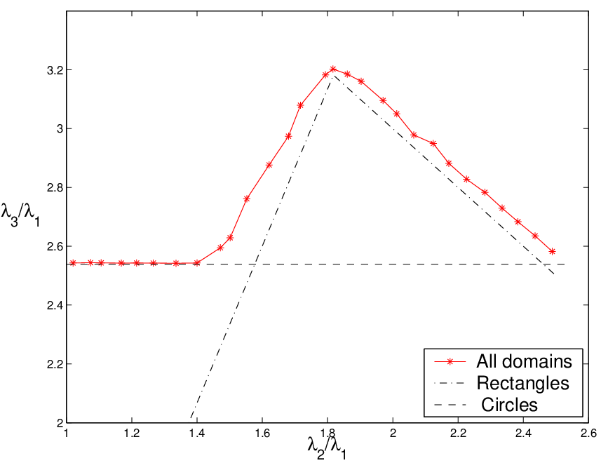
4 Asymptotic results
In this Section, using standard perturbation techniques, we establish several results which, although don’t give the full answer to the question of maximizing the ratio among all planar domains , give some indication which of the domains may or may not be a maximizer. We first proof the following
Theorem 4.1.
The rectangle does not maximize the among all planar domains.** * We were informed by Niculae Mandrache that he had independently obtained a similar result.
This should be compared, however, with Remark 4.6 below.
We also give a proof of the following more general result, which justifies the remark made at the end of last Section.
Theorem 4.2.
Suppose that is a local maximizer of among planar domains with sufficiently smooth boundary. Then .
We should emphasize here that neither the statement not the proof (found below) of Theorem 4.2 is fully rigorous. In the former, we do not discuss the requirements on the smoothness of the boundary and the concept of a local maximizer; we also do not prove that maximizers actually exist. In the latter, we rely on the following unproven, although very plausible, conjecture.
Conjecture 4.3.
Let be a simple eigenvalue of the Dirichlet Laplacian on a planar connected domain. Then not all nodal lines of the corresponding eigenfunction are closed.
Such a conjecture is not unreasonable since, in general, it is quite difficult to construct domains for which even one nodal line of a low eigenfunction is closed, see [HoHoNa].
Before giving the proofs of Theorems 4.1 and 4.2, we recall, without proof, some classical results from the domain perturbation theory. The details can be found, e.g., in [Rel, SHSP].
Domain perturbations
For simplicity, we restrict ourselves to domains in ; all the results stated here hold in any dimension.
Consider, for small values of real parameter , a family of bounded domains in of variable , which are transformed by the change of coordinates
| (4.1) |
into the domain in of variable . We assume that the boundary and the vector-function are sufficiently smooth.
Let be the outer unit normal to , and denote
(in fact, is a smooth function on which gives, up to the leading order for small , the normal distance between and ).
Denote by the eigenvalues of the Dirichlet Laplacian on and by the corresponding basis of normalized orthogonal eigenfunctions (which are chosen real). Also, denote by the eigenvalues of the Dirichlet Laplacian on . For sufficiently small , the are continuous functions of and tend to as .
The following two results go back to Rellich.
Proposition 4.4.
Let , , be a simple eigenvalue of the Dirichlet Laplacian on . Then has the asymptotic expansion
| (4.2) |
as , where
| (4.3) |
The situation is slightly more complicated when is an eigenvalue of multiplicity . For simplicity, we consider just the case .
Proposition 4.5.
Let be a double eigenvalue of the Dirichlet Laplacian on . Then, as , and still have the asymptotic expansions (4.2) () with
| (4.4) |
where , are two real roots of the quadratic equation
| (4.5) |
and
| (4.6) |
We will be in fact interested in the asymptotic expansion of , which follows from (4.2):
| (4.7) |
Proof of Theorem 4.1
Let be the rectangle . We shall construct an explicit perturbation using (4.1) such that the first correction term in the asymptotic formula (4.7) is positive for , and therefore for sufficiently small positive .
Let
where
We will choose the coefficients later.
The corresponding function appearing in the asymptotic formulae above is
Note that we shall use (4.3) for computing and (4.4) for computing and , since is a double eigenvalue of the unperturbed problem. Elementary but tedious calculations show that the correction terms , , depend only upon the parameters with . For brevity, we omit the explicit expressions.
Let us choose the parameters in such a way that (i.e., remains a double eigenvalue up to the linear terms in ). This, by Proposition 4.5, happens when and , which in turn leads to the following conditions on coefficients :
| (4.8) |
Under conditions (4.8), asymptotic formula (4.7) simplifies dramatically, and becomes
and we can choose and in such a way that its right-hand side is positive for sufficiently small positive . This proves Theorem 4.1.
Remark 4.6.
Let be any rectangle and consider the perturbations as above but with function linear in (and, naturally, replacing throughout). Thus, we are considering quadrilaterals which are small perturbations of the rectangle . The same elementary calculations then imply that, for and , we obtain, up to and inclusive of the terms of order , that
where is given by the right-hand side of (2.1). In other words, up to the terms of order the rectangles are local maximizers among all quadrilaterals which are sufficently “close” to them, cf. Remark 3.1.
Proof of Theorem 4.2
Suppose that is a planar domain with sufficiently smooth boundary which locally maximizes the ratio in the following sense: for any sufficiently smooth perturbation determined by (4.1) we have
| (4.9) |
Assume additionally that is a simple eigenvalue of the Dirichlet Laplacian in the unperturbed domain . We shall show that this assumption leads to the contradiction with Conjecture 4.3.
Since both and are simple eigenvalues, the asymptotic formula (4.7) becomes, in accordance with Proposition 4.4,
Now, as can be chosen both positive and negative, (4.9) can hold only if
and since is an arbitrary smooth function, this requires
everywhere on . But the normal derivative of the first eigenfunction of the Dirichlet Laplacian is non-zero everywhere on the boundary, so the last formula implies that the third eigenfunction has the same property, and therefore all its nodal lines are closed, in contradiction with Conjecture 4.3.
5 Final Remarks
On the basis of the numerical computations and the results proven above we make the following conjecture, most of which is still to be established (or disproved) rigorously:
The domain maximizing the ratio for planar domains is close in shape to the optimal computed dumbbell-shaped domain shown in Fig. 9, is simply-connected, and has a smooth boundary. The maximal admissible value is approximately equal to or is slightly greater than .

References
- [Ash] Ashbaugh, M S, Isoperimetric and universal inequalities for eigenvalues, in Spectral theory and geometry (Edinburgh, 1998), E B Davies and Yu Safarov, eds., London Math. Soc. Lecture Notes, vol. 273, Cambridge Univ. Press, Cambridge, 1999, pp. 95–139.
- [AshBen1] Ashbaugh, M S and Benguria, R D, Proof of the Payne-Pólya-Weinberger conjecture, Bull. Amer. Math. Soc. 25 (1991), 19–29.
- [AshBen2] Ashbaugh, M S and Benguria, R D, Isoperimetric bound for for the membrane problem, Duke Math. J. 63 (1991), 333–341.
- [AshBen3] Ashbaugh, M S and Benguria, R D, A sharp bound for the ratio of the first two eigenvalues of Dirichlet Laplacian and extensions, Annals of Math. 135 (1992), 601–628.
- [AshBen4] Ashbaugh, M S and Benguria, R D, Isoperimetric bounds for higher eigenvalue ratios for the -dimensional fixed membrane problem, Proc. Royal Soc. Edinburgh 123A (1993), 977–985.
- [AshBen5] Ashbaugh, M S and Benguria, R D, The range of values of and for the fixed membrane problem, Rev. in Math. Phys. 6 (1994), 999–1009.
- [AshBen6] Ashbaugh, M S and Benguria, R D, Bounds for ratios of first, second and third membrane eigenvalues, in Nonlinear Problems in Applied Mathematics: In Honor of Ivor Stakgold oh his Seventieth Birthday, T S Angell, L P Cook, R E Kleinmann, and W E Olmstead, eds., Society for Industrial and Applied Mathematics, Philadelphia, 1996, pp. 30–42.
- [FEMLAB] FEMLAB 2.0 User’s Guide and Introduction, Comsol AB, 2000, see also http://www.femlab.com.
- [Hae] Haeberly, J-P, On shape optimizing the ratio of the first two eigenvalues of the Laplacian, Computer Science, Technical Report 586, Courant Institute, New York University, 1991.
- [HaeOve] Haeberly, J-P and Overton, M L, A hybrid algorithm for optimizing eigenvalues of symmetric definite pencils, SIAM J. Matrix Anal. Appl. 15 (1994), 1141-1156.
- [HarStu] Harrell, E M, II and Stubbe, J, On trace identities and universal eigenvalue estimates for some partial differential operators, Trans. Amer. Math. Soc. 349 (1997), 2037-2055.
- [HiPr] Hile, G N and Protter, M H, Inequalities for eigenvalues of the Laplacian, Indiana Univ. Math. J. 29 (1980), 523-538.
- [HoHoNa] Hoffmann-Ostenhof, M, Hoffmann-Ostenhof, T and Nadirashvili, N, The nodal line of the second eigenfunction of the Laplacian in can be closed, Duke Math. J. 90 (1997), no. 3, 631–640.
- [LevPar] Levitin, M and Parnovski, L, Commutators, Spectral Trace Identities, and Universal Estimates for Eigenvalues, J. Funct. Anal. (2002), to appear.
- [PDETool] Partial Differential Equation Toolbox User’s Guide, The MathWorks, Inc., 1995, see also http://www.mathworks.com.
- [PPW] Payne, L E, Pólya, G, and Weinberger, H F, On the ratio of consecutive eigenvalues, J. Math. and Phys. 35 (1956), 289–298.
- [Rel] Rellich F, Perturbation Theory of Eigenvalue Problems, Gordon and Breach, New York, 1969.
- [SHSP] Sanchez-Hubert, J and Sanchez-Palencia E, Vibration and Coupling of Continuous Systems – Asymptotics Methods, Springer-Verlag, Berlin, 1989.
- [Yan] Yang, Hongcang, An estimate of the difference between consecutive eigenvalues, preprint IC/91/60 of the Intl. Centre for Theoretical Physics, Trieste, 1991 (revised preprint, Academia Sinica, 1995).