Laminations and groups of homeomorphisms of the circle
Abstract.
If is an atoroidal 3-manifold with a taut foliation, Thurston showed that acts on a circle. Here, we show that some other classes of essential laminations also give rise to actions on circles. In particular, we show this for tight essential laminations with solid torus guts. We also show that pseudo-Anosov flows induce actions on circles. In all cases, these actions can be made into faithful ones, so is isomorphic to a subgroup of . In addition, we show that the fundamental group of the Weeks manifold has no faithful action on . As a corollary, the Weeks manifold does not admit a tight essential lamination, a pseudo-Anosov flow, or a taut foliation. Finally, we give a proof of Thurston’s universal circle theorem for taut foliations based on a new, purely topological, proof of the Leaf Pocket Theorem.
1991 Mathematics Subject Classification
57M25, 57M501. Introduction
Let be an atoroidal 3-manifold with a taut foliation . The foliation gives rise to actions of on 1-manifolds in two ways: the action on the space of leaves in the universal cover, and the action on a universal circle. These actions are very useful for understanding . If is an atoroidal -manifold with an essential lamination, one still has an action of on the space of leaves in the universal cover, but this space is just an order tree, not a 1-manifold. Our main goal here is to give analogues of the second kind of action: we construct actions of fundamental groups of -manifolds on circles arising from certain kinds of essential laminations. Before giving precise statements, we’ll discuss the case of taut foliations.
Let denote the universal cover of , and the foliation of covering a taut foliation of . First, consider the leaf space of . The space is simply connected and locally homeomorphic to , but is typically non-Hausdorff. We will still refer to as a 1-manifold. There is a natural action of on , and this action has no global fixed point. In fact, after changing slightly by a monotone equivalence, we can ensure that the homomorphism is injective (see Theorem 7.10). Thus is isomorphic to a group of homeomorphisms of a 1-manifold.
Second, Thurston has shown that the foliation gives rise to another action of on a 1-manifold, namely on a universal circle. This circle, , is constructed by collating the circles at infinity of the leaves of . As in the previous case, the action on a universal circle is faithful (Theorem 6.3). Thurston’s paper [Thu] on this topic is largely unwritten, so we provide a complete proof here. The main technical tool for proving the existence of a universal circle is Thurston’s Leaf Pocket Theorem. This theorem says, very roughly, that the leaves of come together in many directions. Thurston’s proof of this theorem is analytic, and uses theorems of L. Garnett on the existence and quality of harmonic transverse measures for foliations. We give a new and purely topological proof of a slight variation of the Leaf Pocket Theorem, Theorem 5.2, which applies more generally to essential laminations. In Section 6, we use Theorem 5.2 to prove the existence of universal circles.
Now we will outline our results for essential laminations. For background and more detailed definitions see Section 2. An essential lamination of a 3-manifold is tight if the leaf space of is Hausdorff. Equivalently, leaves of are uniformly properly embedded in . The complementary regions of can be partitioned into interstitial regions and guts. The interstitial regions are (typically noncompact) -bundles whose -bundles lie on , and the compact guts make up the rest of the complement.
Our main result is
3.2 Theorem.
Let be an atoroidal 3-manifold containing an essential lamination . If is tight and all the gut regions are solid tori, then has a faithful action on .
Here’s an outline of the proof. We can assume that has non-empty guts (i.e. is genuine), as otherwise it can be blown down to a taut foliation which gives rise to an action on a universal circle. The first step in the proof is the following lemma, which is of independent interest:
4.1 Filling Lemma.
Let be a -manifold and a genuine lamination all of whose guts are solid tori. Then there is a genuine lamination containing , whose complementary regions are all ideal polygon bundles over . Moreover, if is tight, so is .
A lamination such as whose complementary regions are all ideal polygon bundles is said to be very full. A good example to keep in mind of a very full lamination is the suspension of the stable lamination of a pseudo-Anosov surface homeomorphism in the corresponding surface bundle.
The Filling Lemma 4.1 reduces the proof of Theorem 3.2 to the case where is tight and very full, which is handled in Theorem 3.1. The basic idea is to flatten out into a geodesic lamination of , taking care so that inherits a group action of which is equivariant with respect to the map . The action of on induces an action on the circle at infinity of , which is the desired circle action.
We can lessen the requirement that be tight somewhat, when the non-Hausdorff behavior of the lamination is not too bad. See Section 3.4 and Theorem 3.8. In particular Theorem 3.8 applies to the stable or unstable lamination of a pseudo-Anosov flow. Thus (Corollary 3.9) fundamental groups of 3-manifolds with pseudo-Anosov flows also act faithfully on the circle.
1.1. Nonexistence results
Given the results above, it is natural to ask the question: Which atoroidal 3-manifolds have faithful circle actions? We show that not every 3-manifold has such an action. In particular, for the closed hyperbolic 3-manifold with smallest known volume, we have:
9.2 Theorem.
The fundamental group of the Weeks manifold does not act faithfully on the circle.
As a corollary of this and the above theorems on the existence of circle actions, it follows that the Weeks manifold does not admit a tight essential lamination with solid torus guts, a pseudo-Anosov flow, or a taut foliation. Using Agol’s volume estimates for manifolds with tight laminations [Agol], one can show that any tight lamination in the Weeks manifold would have solid torus guts. So we have the stronger conclusion that the Weeks manifold contains no tight essential lamination (Corollary 9.4). We conjecture that the Weeks manifold contains no essential lamination at all, but this remains open. Also, the fundamental group of the Weeks manifold appears to be the first known example of a rank-1 lattice which cannot act faithfully on the circle. In contrast, Witte has shown that there are many higher rank lattices with this property [Wit].
Examples of hyperbolic manifolds without taut foliations were already known from the breakthrough work of Roberts, Shareshian, and Stein [RSS]. In fact, they constructed infinitely many such examples by looking at certain Dehn fillings of punctured torus bundles with negative trace. They showed the non-existence of taut foliations by proving that the fundamental groups of these manifolds can’t act on a simply-connected 1-manifold without a global fixed point. Given the multitude of non-Hausdorff 1-manifolds, it is remarkable that such a proof can be made to work. One of our original motivations for this paper was to reprove non-existence of taut foliations by studying only actions on Hausdorff 1-manifolds, in particular actions on .
The technique used for proving Theorem 9.2 is this. Let be the fundamental group of the Weeks manifold. First, we pass to a finite index subgroup where the action on lifts to an action on . A faithful action of on is equivalent to a left-invariant total order on (see Section 7). The non-existence of such an order is then shown by considering various possibilities for which elements of satisfy . For some -manifold groups this can be done algorithmically as discussed in Section 8. While the Weeks manifold was the only case where we managed to show that the fundamental group doesn’t act faithfully on the circle, we found many examples in the Hodgson-Weeks census whose fundamental groups can’t act faithfully on (see Section 10).
1.2. Further Questions
Because essential laminations are very common, these results show that many 3-manifold groups are subgroups of . So a natural question is: Suppose that is a subgroup of . What does this tell us about the algebraic properties of ? Of course, a general finitely generated subgroup of can be quite strange, e.g it can contain Thompson’s infinite simple group. However, the actions we construct have additional special properties; for instance, they preserve the endpoints of a special kind of geodesic lamination of . So one can hope that the existence of such an action implies something interesting about .
1.3. Acknowledgments
The first author was at Harvard University when this work was done, and was partially supported by an NSF VIGRE grant. The second author was partially supported by an NSF Postdoctoral Fellowship. We thank Bill Thurston, Rachel Roberts, and Ian Agol for useful conversations. We also thank Sergio Fenley and the referee for their comments and suggestions on an earlier draft of this paper. The main results in this paper were announced in a minicourse by the first author at a conference at P.U.C. in Rio de Janeiro in August 2001. The first author would like to thank the P.U.C. for their hospitality.
2. Background on essential laminations
In this section, we summarize the definitions and some of the basic results about taut foliations and essential laminations (for more detail see the references in [Gab]). Throughout, will be a closed 3-manifold. We’ll begin with taut foliations:
2.1 Definition.
Let be a foliation of by surfaces. The foliation is taut if there is a loop in transverse to which intersects every leaf.
We will use to denote the induced foliation of the universal cover of . The leaf space of is a simply-connected, not necessarily Hausdorff, -manifold. Some basic properties of manifolds with taut foliations are summarized in the following theorem:
2.2 Theorem (Novikov, Rosenberg, Reeb).
Let be a -manifold with a taut foliation . Then either is finitely covered by , and is finitely covered by the product foliation by spheres, or foliated by planes. In particular, every leaf of is incompressible, and every loop transverse to is homotopically essential.
A codimension one lamination of is a foliation of a closed subset, i.e. a closed union of complete embedded surfaces—the leaves of the lamination—which intersect small open charts of in products of the form , where is any closed subset of an interval, and each leaf locally intersects the open set as a horizontal slice . Globally, of course, a leaf might intersect a product chart in infinitely many horizontal slices. Typically, consists of a union of intervals, isolated points, and Cantor sets. Generalizing the notion of tautness for foliations is:
2.3 Definition.
A lamination is essential if each complementary region is irreducible and has boundary which is incompressible and end-incompressible. Moreover, we require that no leaf of is a 2-sphere, or a torus leaf bounding a Reeb component.
Here a leaf is end-compressible if it has an end-compressing monogon—that is, a monogon properly embedded in a complementary region which is not homotopic (rel boundary) into . An end-compressing monogon is an obstruction to finding a metric with respect to which leaves of are minimal surfaces; excluding such monogons ensures that essential laminations share many properties in common with taut foliations. In particular, manifolds with essential laminations have universal cover and any tight transversal is homotopically essential (see [GO]).
For an essential lamination, we can define the leaf space of , but this is now just an order tree, not a 1-manifold; the vertices of are the set of non-boundary leaves of together with the set of closed complementary regions. If this leaf space is Hausdorff, we say is tight. This is equivalent to the leaves of being uniformly properly embedded in . That is, there is a proper increasing function such that if and are distance apart in the path metric on , then and are at least distance apart in . When is a foliation, tightness is equivalent to the leaf space being .
Regardless of whether is tight, we have the following simple fact:
2.4 Lemma.
Let be an essential lamination. Then there is an such that every leaf of is quasi-isometrically embedded in its -neighborhood. Such an is called a separation constant for .
Proof.
By compactness of , we can pick an so that every ball of radius in is contained in a product chart. Here, by “product chart” we also require that every transverse arc without backtracking and with endpoints in is tight, that is, can’t be homotoped rel endpoints into a leaf. Note that in any leaf intersects a product chart at most once, as otherwise we can build a tight transversal loop to by starting with a transversal in the chart and an arc in .
Now consider the -neighborhood of a leaf in . We can cover the larger neighborhood by a product charts . As noted above, intersects each of these charts only once. Because is compact, each of these charts has bounded geometry. Therefore, is quasi-isometrically embedded in . ∎
2.5. Complementary regions
Let be a complementary region to an essential lamination . We will consider decompositions of along a union of properly embedded annuli into two kinds of pieces, guts and interstitial regions. By definition, gut regions are compact and interstitial regions are -bundles over (typically noncompact) surfaces. The annuli of the decomposition are called the interstitial annuli, and we require that no two of them are isotopic in a gut region. By convention, if is itself an -bundle over a closed surface, the only allowed decomposition is the trivial one with all of being the interstitial region.
Such a partition of into guts and interstices need not be unique: if is an interstitial region over a surface , and if is a compact subsurface of (possibly with boundary), then the subset can be included into the gut. Conversely, an -bundle over a compact surface which is contained in the gut can be included into the interstitial region. However, there exist several canonical (up to isotopy) partitions of into guts and interstices. One such canonical partition has the property that every interstitial region is an -bundle over a non-compact surface (see [GO] or [GK3] ).
Often, it’s useful to make the distinction between essential laminations and genuine ones:
2.6 Definition.
An essential lamination is genuine if some complementary region is not an -bundle. Equivalently, there is a decomposition of the complementary regions with non-empty guts.
An essential lamination which is not genuine can be filled in to a foliation by adding leaves in the complementary -bundles.
One way to think of the qualities essential and genuine for a lamination is in terms of the proper essential surfaces (with boundary) contained in a complementary region. A lamination is essential if the complement admits no essential sphere, disk or monogon; that is, it contains no essential surface of positive Euler characteristic. An essential lamination is genuine if some complementary region contains an essential surface of negative Euler characteristic.
The following is an example of a genuine lamination which is a good example to think about throughout this paper.
2.7 Example.
Let be a surface bundle over the circle with fiber and pseudo-Anosov monodromy . There are a pair of geodesic laminations of invariant under , the stable and unstable laminations . Since these are invariant, they suspend in the mapping torus to a pair of laminations of transverse to the surface fibration. The complementary regions of the geodesic laminations of suspend to complementary regions of . The complementary regions in are finite sided ideal polygons, each with at least sides. These suspend to ideal polygon bundles over . Such complementary regions decompose into compact neutered ideal polygon bundles over (the guts) and cusps (the interstitial regions). In particular, these laminations are genuine. In , the pair is a product . As is a geodesic lamination, the leaf space of is Hausdorff. Thus the leaf space of is also Hausdorff, and is tight.
2.8. Tangential geometry
The tangential geometry of an essential lamination is controlled by the following theorem of Candel [Can1], which can be thought of as a uniformization theorem for Riemann surface laminations:
2.9 Theorem (Candel).
Let be a Riemann surface lamination such that for every transverse measure we have:
Then there is a continuously varying leafwise metric on where the leaves are locally isometric to .
A lamination satisfying the conclusion of Candel’s Theorem is said to have hyperbolic leaves. For an essential lamination of an atoroidal -manifold, every transverse measure has negative Euler characteristic, and so has hyperbolic leaves.
Now we restrict attention to a taut foliation . Candel’s Theorem is very useful in understanding the following bundle:
2.10 Definition.
Let be a taut foliation. The circle bundle at infinity, , is the circle bundle over whose fiber over a leaf is the circle .
While the bundle is easy to understand as a set, its topology requires some discussion. We topologize it as follows. For each transversal to , the projection of to is an embedding, so it makes sense to talk about the restriction . Consider the restriction to of the unit tangent bundle of , denoted . For a point , every vector determines a point by taking the endpoint of the geodesic ray in starting at in direction . Thus there is a bijection
We topologize by declaring that this map is a homeomorphism for each .
We verify that this is well-defined. Suppose and are two transversals with the same projection to . For each leaf , the map
is determined by the geometry of a compact disk containing the points and . In particular, since the geometry of the leaves intersecting the varies continuously on compact subsets, the map
is a homeomorphism. Thus the topology of is well-defined.
This may seem like a tedious verification, but there actually is a subtle point here. This construction uses in an essential way the full power of Candel’s Theorem. If we merely knew that the leaves of were uniformly coarsely quasi-isometric to , the map between unit tangent circles would depend on the global geometry of the leaf , and not merely on the local geometry. But in general, the leaves do not vary continuously as subsets of in any reasonable sense. This is the very subtlety that makes Candel’s theorem nontrivial. There is an alternate construction of the topology of without invoking Candel’s theorem, but it is more involved, and uses the Leaf Pocket Theorem 5.2.
3. Tight laminations
In this section, we prove that certain kinds of tight genuine laminations give rise to faithful actions on the circle. Recall that a genuine lamination is very full if the complementary regions are all finite-sided ideal polygon bundles over . Our basic result here is:
3.1 Theorem.
Let be an orientable atoroidal -manifold containing a very full essential lamination which is tight. Then there is a faithful representation
Moreover, the image of preserves a dense lamination of .
Here, a lamination of is essentially just a geodesic lamination of . Intrinsically, is a closed, symmetric subset of so that no two pairs of points and in are linked on .
The hypothesis of very full is much stronger than just having solid torus guts; the former requires in addition that the interstitial regions have as little topology as possible. An typical example of a lamination with solid torus guts which is not very full is depicted in Figure 4.3. However, the Filling Lemma 4.1 shows that a lamination with solid torus guts can be included as a sublamination of a very full lamination. Moreover, this process preserves tightness. So as an immediate consequence of the Filling Lemma and Theorem 3.1 we have:
3.2 Theorem.
Let be an orientable atoroidal -manifold, and a tight lamination with solid torus guts. Then has a faithful representation into .
While the restriction of solid torus guts might initially seem quite strong, in fact many constructions of essential laminations yield examples of this type. Moreover, for non-Haken manifolds, the gut regions are always handlebodies of some sort [Bri1].
Now let’s prove Theorem 3.1.
Proof of Theorem 3.1.
For any essential lamination , the universal cover is topologically , and the lifted lamination is topologically a product of a lamination of with [GK1]. Moreover, the leaves of are proper. Thus is quite close to being a geodesic lamination of . As our is very full, the complementary regions of are all finite-sided ideal polygons. In essence, we’ll construct an action of on so that the map is equivariant, and from this we’ll get the required action on a circle. As is very full, the complementary regions of are all products for finite sided ideal polygons . When turning into a product, there are essentially two possible ways of flattening each into a complementary region of . The key to constructing the desired action on is to do this flattening in a consistent, equivariant way.
So let’s begin the actual construction, which involves fitting the together as ideal polygons in the unit disk. First, downstairs in , choose an orientation on the core curve of each complementary region of . Lifting upstairs, this defines a (dual) orientation on each which is preserved by the action of . As with any essential lamination, there is a natural leaf space associated to . The leaf space is an order tree associated to whose vertices are the set of non-boundary leaves of together with the set of closed complementary regions. This order tree can be canonically included in an -order tree (see e.g. [GK2]); this makes the explanation of the construction easier to follow, so we suppose this has been done. As is tight, is Hausdorff.
We will insert the as ideal polygons in the unit disk via a map which satisfies the following conditions:
- (1)
If , then the closed polygons and are disjoint.
- (2)
The circular ordering on the vertices of induced by agrees with that arising from the orientation on .
- (3)
Suppose is joined to by an embedded arc in joining a side of to a side of . Then the corresponding edges and separate the interiors of and in .
Here’s how to construct . Because the -order tree is Hausdorff, it is the union of a countable number of finite simplicial trees [GK2, §3]. Here, is subdivided and extended to get . Consider as a simplicial complex with no edges of valence two. Each interior vertex of corresponds to some complementary region of , and thus to some . The edges of coming into a vertex correspond to the edges of the associated . Thus, the orientation on induces a cyclic ordering of the edges around each vertex of . There is a unique embedding of into the interior of which respects these cyclic orderings (i.e. at each vertex of the ordering of edges agrees with the clockwise ordering of the image edges about ). For each vertex in , place the corresponding as an ideal polygon in so that it contains . The resulting polygons satisfy (1-3), and moreover their placement was unique up to homeomorphism of . Inducting up the gives us the required map .
Now, the closure
might not be all of , but the components of are easy to understand. Any component of is a polygon whose sides alternate between arcs of and geodesics in which are limits of edges in . Moreover, we claim must be a quadrilateral. To see this, pick one in each component of and join them by a finite simplicial tree in . Embedding in , we see that if there were more than two components to , then would have to have a vertex in .
If we quotient out by collapsing the arcs in to points, we get a circle because has no isolated leaves. Let be this monotone quotient map. The closure of the edges of the is a geodesic lamination of . The map gives a map on pairs of endpoints of geodesics of which preserves unlinking, so there is a well-defined image lamination in . The endpoints of leaves of are dense in . The action of on induces an action on . Going back to our original construction of , it is not hard to see that this extends to a continuous action on which preserves orientation.
To finish the proof, we need show this action is faithful. Consider a nontrivial element which acts trivially on . Then the action of on would stabilize every complementary region. So defines the core curve of every complementary region. It follows that is central in , and that contains a . This violates our assumption that is atoroidal. Thus we have constructed the required faithful action on a circle. ∎
3.3. Flips
If there are complementary regions to , the above construction gives representations which are pairwise non-conjugate in (they fall into only conjugacy classes in the full group ).
Abstractly, this reflects an interesting operation on representations of groups
whose image preserves a lamination of . Given an orbit class of complementary regions to , we get a new representation as follows. Let be a complementary region of . We can “cut” along the edges of each translate into pieces which are itself, and the pieces on the other sides of the boundary edges of . Then we can reverse the orientation of and glue the other pieces back so that each pair of sides is glued in the same way as before, but the relative orientations are now switched. Do this in some order for each , to get a new lamination on which acts. This action extends in the obvious way to a representation . Note that and for any . We call this operation the flip of along .
If only has one orbit class of complementary region, this operation merely reverses the orientation of , but in general it seems somewhat mysterious. It might be interesting to analyze this operation for some familiar . For instance, one could look at for a hyperbolic -manifold fibering over , and the lift of the stable lamination of the monodromy of the fibering.
The moral of these examples is that if a group acts on a (-, order-) tree and there is at least one way of embedding in the plane in a -equivariant way, there are usually many such ways.
In the sequel, we will be interested in obtaining representations of in with Euler class equal to (see Section 7). We suspect the flip operation might be a useful tool in this regard. It is not hard to see that if has equivalence classes of complementary polygons, there is an expression of as a sum
such that the Euler class of is
3.4. Laminations and cataclysms
The rest of this section is devoted to generalizations of Theorem 3.2 where we partially relax the requirement that the lamination be tight. To start, we need to get a handle on what a non-tight lamination looks like.
If is not tight, by definition the leaf space of is a non-Hausdorff order tree. Recall that two leaves and in are comparable if they can be jointed by a tight transversal, and incomparable otherwise. A sequence of leaves in is monotone ordered if all of the lie in an ordered segment , so that the form an increasing sequence in . We define a cataclysm to be a collection of incomparable leaves of , called the limit leaves, for which there is a monotone ordered sequence , called the approximating sequence, which converges on compact subsets in the Hausdorff topology to the union of the ; that is, for all compact subsets ,
in the Hausdorff topology on closed subsets of .
For any sequence which converges to some , the sequence of pointed metric spaces converges to . In particular, if and are two sequences with where and for , then the leafwise distance from to in goes to infinity.
We define an equivalence relation on cataclysms as follows: two cataclysms and are equivalent if and are equal as sets, and if for some , the union
can be totally ordered in .
The equivalence class of a cataclysm is determined by the collection of leaves, since for any and any contained in on the side of which contains the other , the leaves with are an approximating sequence, unique up to equivalence. It follows that the stabilizer of a cataclysm acts by permutations on the set of limit leaves, and by isometry on their union, thought of as a subset of .
The following condition is natural for trying to build circle actions:
3.5 Definition.
A lamination has orderable cataclysms if for each equivalence class of cataclysm , there is an ordering on the set of limit leaves of which is invariant under the action of the stabilizer of in .
We will show that orderable cataclysms can replace tight as a hypothesis in Theorem 3.2, but let’s first give an example of this condition.
3.6 Example.
Let be a pseudo-Anosov flow, and denote the two dimensional stable and unstable singular foliations and . For ease of notation, we will focus on but of course similar statements are true for . The foliation lifts to a singular foliation of invariant under the lifted flow . Each nonsingular leaf of is topologically a plane foliated by flow lines of . If is a nonsingular leaf of , the flow along by compresses the flowlines together. Thus the holonomy along this foliation is defined in the positive direction for all time. In particular, it is easy to see from this that is isometric to . The foliation is a foliation of by geodesics asymptotic to a unique point in . A singular leaf of has the following structure. Let be copies of foliated by geodesics asymptotic to , and let be one of these geodesics. Then separates into two sides, . We obtain a quotient space
by gluing to via an isometry taking to , where the indices are taken modulo . Then , and the are called the faces of the singular leaf . The image of the in is a singular orbit of and covers a circular singular orbit in .
The singular foliation can be split open into a lamination whose leaves are exactly the nonsingular leaves of the together with one leaf for every face of a singular leaf. If is pseudo-Anosov but not Anosov, then is a very full genuine lamination, and if is Anosov then . The foliation of the leaves of by flow lines of gives rise to foliations of the leaves of . Consider a cataclysm with limit leaves and approximating sequence . The foliations of the by flowlines of converge on compact sets to the foliations of the . So if we pick points so that is very close to , there is a natural order on the coming from the order on the leaf space of the foliation of , which is . This determines an order on the indices . As , the order on the indices is eventually constant, and therefore determines a natural order on the set , which is invariant under the stabilizer in of . Thus has orderable cataclysms.
This natural order structure on the cataclysms of pseudo-Anosov flows was observed by Fenley in [Fen], where he gives examples of pseudo-Anosov flows where is not tight.
3.7 Example.
Not all cataclysms are orderable. Here is a simple example. Start with a tight lamination with a complementary region which is an ideal square bundle over the circle where the monodromy is the rotation through angle . Then fill in that region with a saddle bundle over . In the universal cover, the bundle of saddles lifts to leaves which limit in either direction to a pair of distinct leaves corresponding to opposite sides of the ideal square. Either end gives a cataclysm with two limit leaves. The stabilizer of the cataclysm corresponds to the monodromy of the core of the complementary region downstairs; in particular, it interchanges these two limit leaves, and this cataclysm is not orderable.
Now we’ll show:
3.8 Theorem.
Let be an orientable atoroidal -manifold containing a lamination with solid torus guts and orderable cataclysms. Then has a faithful representation in .
Proof.
By the Filling Lemma 4.1, can be filled to a very full lamination. The proof that filling preserves tightness further shows that filling preserves the set of equivalence classes of cataclysms, and that no added leaf is a limit leaf of a cataclysm. In particular, the filled lamination has orderable cataclysms. So from now on, we’ll assume that is very full.
The proof is now morally the same as for Theorem 3.1, but this time it’s easier to do things a little more abstractly. A circular order on a set is an assignment to each triple of distinct elements an orientation of clockwise or anti-clockwise, satisfying the obvious rules coming from triples of points on . Here, we will show that the set of ends of has a natural circular order which is invariant under the action of . We will complete with respect to this circular order to get the needed circle. (For a detailed definitions and basic properties of circular orders on sets and left-invariant circular orders on sets acted on by a group, see e.g. [Tar].)
By definition, a circular order on an order tree consists of two things: a circular order on sets of segments with only a vertex in common, and a linear order on sets of segments which differ only by a vertex (for details see [GK2]). For the leaf space of our lamination we can define a circular order which is invariant under the action of as follows. A set of segments with only a vertex in common corresponds to the set of faces of a closed complementary region of . As before, if we fix orientations of the core curves of the complementary regions , the faces of have a natural circular order. A set of segments which differ only in a vertex corresponds to a cataclysm, and so has an order by assumption. In the cataclysm case, we can certainly choose our orderings to be -equivariant.
Thus is an order tree with a -invariant circular order. Let be the set of ends of . If are three distinct ends in , we define their circular order as follows. Take any point in and consider rays starting at and ending at . By looking at the (circularly ordered) subtree , we get a circular order of the ends of the . This order is independent of the choice of point , and so we have a natural circular order on which is invariant under the action of . Up to homeomorphism, there is a unique way to embed into a circle so that the embedding respects the circular orderings and is continuous with respect to the topology on induced by the order. The closure of the image of may omit some gaps, which we can collapse to get the promised circle on which acts. As in the proof of Theorem 3.1, if some element acts trivially on this circle, it must fix every complementary domain; then has a nontrivial center, violating the assumption that is atoroidal. ∎
3.9 Corollary.
Let be an atoroidal -manifold which admits a pseudo-Anosov flow . Then admits a faithful representation in .
Proof.
If is pseudo-Anosov but not Anosov, the singular unstable foliation can be split open to a very full genuine lamination. As explained in Example 3.6, these laminations have orderable cataclysms and so Theorem 3.8 applies. If is Anosov, the unstable foliation is a taut foliation, and the circle action comes from Theorem 6.3. ∎
3.10. Invariant laminations for cataclysms
For the sake of completeness, we give a more precise description of the non-Hausdorff behavior of the leaf space at a cataclysm. The following theorem shows that the set of limit leaves of a cataclysm can be parameterized by a geodesic lamination of in a (topologically) canonical way.
3.11 Theorem.
Let be an essential lamination, and let be a cataclysm of . Then we can associate a lamination of to in such a way that the complementary regions to are in - correspondence with the limit leaves of , and the stabilizer of acts by homeomorphisms of which preserve , and permute the complementary regions by the permutation action on the limit leaves of .
Proof.
For each limit leaf , pick some point , and for each approximating leaf pick such that the limit to as , for each . Pick some small , and consider for each limit leaf and each approximating leaf the subspace consisting of points which are within of . Then for sufficiently small , the sets and are disjoint for , since for any lamination with bounded geometry, leaves are uniformly properly embedded in their neighborhoods for some , and therefore pairs of points on incomparable leaves of are a uniform distance apart. On the other hand, by the Leaf Pocket Theorem 5.2, for large , contains a -net of points in the circle at infinity in the visual metric as seen from . In particular, the boundary of the convex hull of the limit set of defines a collection of geodesics which separates most of from for in some definite order; the closure of the union of such geodesics is a geodesic lamination of . This lamination is dual to a planar order tree whose vertices are the for which is sufficiently close to . In particular, there are a sequence of inclusions and the union is a Hausdorff planar order tree dual to a lamination of , which is a limit of the under an appropriate sequence of homeomorphisms (not isometries) from . It is clear that does not depend on the choice of approximating leaves, since if we insert some between and then there are inclusions and the limit is unchanged. In particular, depends only on , and therefore the stabilizer of acts on it by automorphisms. ∎
4. The Filling Lemma
This section is devoted to the proof of the following lemma, which is of independent interest. It resolves the disparity between having solid torus guts and solid torus complementary regions, and is used in Section 3 to reduce the construction of actions on circles to the latter case.
4.1 Filling Lemma.
Let be an orientable -manifold and a genuine lamination such that for some decomposition of into interstices and guts, the guts are neutered ideal polygon bundles over . Then can be filled to a genuine lamination , whose complementary regions are all ideal polygon bundles over . That is, is very full. Moreover, if is tight, so is .
Before giving the proof, let us point out another application. Gabai and Kazez have shown that if an atoroidal manifold has a genuine lamination with some complementary region a solid torus, then homotopic homeomorphisms are isotopic [GK1]. The Filling Lemma extends that result to manifolds with genuine laminations where there is a decomposition of with a solid torus gut region. Now we’ll prove the Filling Lemma.
Proof.
First, fill all product complementary regions with foliation. Now, each complementary region of is a union of gut pieces together with a finite collection of interval bundles (the bases of the need not be compact). The are glued to the along the interstitial annuli. The first step of the proof is to add leaves to reduce to the case where each is a trivial -bundle over a surface with a single boundary component. Then, each is attached to a single along one interstitial annulus, and each contains exactly one gut region. After this basic reduction, we’ll add on a product foliation to the boundary leaves of , and perturb it so that the new is an ideal polygon bundle over .
4.2. Basic reduction
First, we’ll insert finitely many leaves so that each -bundle has only one interstitial annulus in its boundary. Let be an -bundle over a base with at least two boundary components. Pick an interstitial annulus bounding , joining it to a gut region . Let and be the leaves of that runs between.

Build a branched surface from , , and , bending as shown in Figure 4.3. The leaf we add will be carried by , and will consist of one copy of glued to stuff parallel to and . Explicitly, take countably many copies of the two leaves and in a product neighborhood, which accumulate only along and . Take the union of this with to get a two-complex which is singular along countably many circles accumulating to the two boundary circles of . Construct a surface carried by by performing a normal sum operation on each singular circle using a consistent orientation. Let be the component of this new surface which contains most of . Add to to get . To decompose the complement of into -bundles and guts, use essentially the same interstitial annuli as for . In the complement of , the -bundle has been split into a with one fewer boundary components, and another -bundle with one boundary component (consult Figure 4.3). Doing this process at most once for each of our original interstitial annuli gives us a new where each has only one boundary component.
Now, we’ll add finitely many more leaves so that each is a trivial -bundle. Suppose some -bundle is nontrivial, and let be the gut region it’s attached to via the interstitial annulus . Let be a copy of the base of sitting in the middle of . Let be an -bundle attached to along . Choose a horizontal surface in which has exactly one boundary component on . Let be the surface created by gluing and together via an annulus in . If we pick so that and are adjacent on , the new lamination has essentially the same guts as . If was also twisted, adding creates a new with two boundary components, so in this case we add a second leaf as in the previous step so that all -bundles still have a single boundary component. In any event, there are now fewer twisted -bundles in the complement of . Thus, after adding finitely many leaves, we can make all of the trivial -bundles over surfaces with one boundary component.
4.4. Main argument
Consider one of our complementary regions . We need to fill so that becomes an ideal polygon bundle over . As a rough outline, we’ll begin by foliating each interstitial region by planes and annuli in a very standard way. Here, by “plane” we really mean a disc with a part of its boundary removed, and similarly for annuli. The induced foliation of each interstitial annulus will consist of a countable collection of circles, and a bunch of lines spiraling out to the circle leaves. Each annulus leaf has a single circle boundary component and many line boundary components. We’ll split open the foliation of each along one of the annulus leaves and glue these foliations together across the gut to enlarge our original lamination . If we glue with care, the new leaves are all either annuli or planes. The new interstitial -bundles will have bases which are annuli of the form , and so the complementary regions are all ideal polygon bundle over .
We’ll begin by constructing the foliation of each interstitial region. Let be an interstitial region , where is has exactly one boundary loop . Let . We will foliate by choosing some representation
so that the induced foliation of as a foliated bundle has the above properties. We will construct from a representation by lifting to . The group acts on , and we can identify with . We’ll want the representation to be faithful, and also that the nontrivial images are hyperbolic elements. Moreover, we’ll need that in the lift
the rotation number of is zero. This way, will have countably many fixed points, and will alternate between being increasing and decreasing on the complementary intervals.
Here’s why such a exists. The group is a free group, possibly on infinitely many generators. First, consider the case where is finitely generated. Note that the set of faithful representations is dense in the space of all representations; this is because it is the complement of
which is a countable union of proper algebraic subvarieties. For the trivial representation , if we look at the trivial lift then the rotation number of is . For near for which is hyperbolic, the rotation number of near is an integer arbitrarily close to . Thus it is , and we can construct the needed . Moreover, by taking a generic representation , we can also require that the stabilizer of all but a countable set of points in will be trivial, and the stabilizer of each element of that countable set will be isomorphic to .
Now suppose is infinitely generated. Put a hyperbolic structure on with geodesic boundary. This gives a faithful representation where the image of the boundary loop is hyperbolic. As is free, there is a some lift of to . While may not have rotation number 0, this time is a primitive element of ; it is easy to construct a homomorphism from to the center of so that the rotation number of is minus that of . Then is the required homomorphism. Note that inherits from the property that only a countable number of points have non-trivial stabilizer, and that when the stabilizer is non-trivial it is .
By viewing as a subgroup of , we foliate by as a flat foliated bundle with holonomy group . As desired, a countable set of leaves in the interior of will be cylinders, and all the rest will be planes. The restriction of the foliation to the annulus is a -dimensional foliation which is a flat foliated bundle over with holonomy generated by (see Figure 4.5).

The points parameterize the leaves of and the leaves of . Of course, if there is with then , so these labels are not unique. Parameterize in such a way that is an unstable fixed point of . So the interior of is an annulus, and the suspension of the point in is a closed loop in which splits into two foliated annuli . The interior of each leaf of is topologically either an annulus or a plane. However, the boundary of each consists of the leaves
For each , the set of boundary components consists of at most a single closed loop and countably many lines if is an annulus, and countably many lines if is a plane.
Now we’ll extend slightly into in the following way. Let , which is topologically a cylinder, and let denote the non-circle boundary components of . Recall denotes the boundary circle of . We split into two foliated annuli along the circle , and we denote the foliations by . See Figure 4.6.

We extend the foliation to a pair of solid tori and which are interval bundles over annuli neighborhoods of in . We foliate these solid tori by the product of the foliations with . This completes our construction of the foliation of the interstitial region .
We do this procedure simultaneously for all the interstitial regions which bound . For each object constructed in , let denote the corresponding object constructed in .
4.7. Gluing the interstitial foliations
We would like to glue the foliated annuli ends of the together to foliate a product neighborhood of (as suggested by Figure 4.6). Consider a pair of interstitial annuli and which are separated by an annulus of . The task is to glue the foliated annulus to the foliated annulus , being careful about the topology of the resulting leaves. Doing the gluing amounts to finding a conjugacy between the dynamics of on and on with the orientation reversed. There are many choices of such conjugacies; the set of fixed orbits of on is a countably infinite discrete sequence accumulating only at , and the set of fixed orbits of on is a countably infinite discrete sequence accumulating only at . These suspend to closed circles in and respectively, which can be glued together. On a complementary interval in and , the dynamics of and have no fixed points, so the set of conjugacies is parameterized by . We need to choose these conjugacies, simultaneously for all adjacent pairs , so that in the resulting foliation the leaves containing the middle leaves are annuli.
Consider one of the leaves , whose boundary lines are denoted . Since all but countably many leaves of each are planes, it is easy to glue so that boundary lines are glued to lines of some which are boundaries of planar leaves of . However, this is not enough to ensure that the new leaf which contains is an annulus. The leaf is built up of pieces which are leaves from the , and so far we’ve only ensured that those pieces that touch are planar. Moreover, we have to worry about whether the planar pieces of could be glued together in a cycle, adding to the fundamental group of . We’ll solve these problems by building up the gluings inductively. More precisely, start by gluing one boundary line of to a planar leaf. Now glue another one, making sure we don’t add any fundamental group. Now glue a boundary component of one of the planar leaves we added to a new planar leaf. Now go work on some other for a bit, etc. At each stage, we can avoid creating any fundamental group since we’ve only made finitely many gluings. We can formalize the order of induction as follows. Note that when we’re done, each leaf will be built up from an annulus and infinitely many planes glued together along lines in their boundaries. The dual graph to the pattern of gluings is a rooted tree , where the root corresponds to the single annulus piece, and every vertex has valence the cardinality of the natural numbers. So start with a finite set of such trees and choose a bijection from the union of their edges to the natural numbers, so that each embedded path from a root vertex outward is labelled by an increasing sequence of numbers. Then do the gluings in the order of the labeling. Since there are only countably many bad choices for any given gluing, we can find a good choice arbitrarily close to any initial guess, and choose them so that the size of the biggest unglued gap goes to zero; thus this process defines the full gluing map of all the annuli pairs .
Next, we’ll “blow air” into along the leaves to get the final lamination. We can extend to a singular foliation by adding a finite set of annuli , parallel to the annuli components of , which end in pairs on the circles . The only singular leaf of is the single branched surface which is the union of the and the . Then is topologically a train-track bundle over with fiber the train-track obtained from an ideal polygon by collapsing the cusps of to single branches. It is clear that can be split open to a bundle over , by Denjoying each leaf before gluing on the annuli . Thus can be split open to a nonsingular lamination with a single complementary region which is an ideal polygon bundle over . Repeating the construction for every complementary region of the original , we obtain a lamination of all of whose complementary regions are ideal polygon bundles over .
4.8. Tightness is preserved
To finish the proof of the Filling Lemma, it remains to check that the construction preserves tightness. We’ll make this clear by getting an explicit description of the quasi-isometry type of the original complementary regions, and understanding how the added leaves are embedded in these regions.
Let be a genuine lamination with solid torus guts, and take a metric on which makes the leaves of hyperbolic. Let be the universal cover of a complementary region. We want to describe its quasi-isometry type (with respect to the induced path metric). Each leaf of is isometric to . The boundaries of interstitial annuli lift to quasigeodesics in leaves of bounding quasiconvex regions which are the lifts of the base surfaces of the interstitial regions. There are only finitely many interstitial annuli, and so the modulus of quasi-isometry of these geodesics is uniformly bounded. The gut regions lift to solid tori of bounded thickness which are contained in bounded neighborhoods of these quasigeodesics in the various boundary leaves of which they border. Thus, up to coarse quasi-isometry, is a tree of hyperbolic planes. That is, it’s obtained from countably many copies of , glued together in pairs along convex subsets bounded by complete geodesics. A finite number of copies of come together along a boundary geodesic, and the pattern of gluings is treelike—every loop in the union is contained in some copy of .
More precisely, each interstitial region is covered by a product which is uniformly quasi-isometric to a region bounded by a collection of complete geodesics. Each leaf of is tiled by isometric copies of the . Pairs of leaves of are glued together along such tiles, and -tuples are glued together around each boundary geodesic of . We can make a graph with two kinds of vertices: the first kind correspond to the boundary geodesics of tiles . The second kind correspond to the tiles themselves . The edges correspond to a choice of a tile and a boundary leaf in that tile. This gives a graph which is a simplicial tree. (Similar trees of hyperbolic planes arise as quasi-isometric models for Cayley graphs of Baumslag-Solitar groups [FM], but there the tiles are glued along regions bounded by horocycles, not geodesics.)
Looking back at our construction, the final lamination was obtained from by inserting new leaves into complementary regions to so that the added leaves are everywhere transverse to the -bundle regions and parallel to the boundary in the gut regions. Such leaves are covered in by hyperbolic planes which project homeomorphically to the slices in our quasi-isometric model. It is clear that a sequence of such slices cannot converge to a pair of distinct slices, and so the leaf space of the leaves inside is Hausdorff. Thus is tight if is. This completes the proof of the Filling Lemma. ∎
5. Leaf pocket theorem
Let be a taut foliation with hyperbolic leaves. Consider a leaf of , and a point in . Given a geodesic ray starting at , we can ask: Can we choose a transversal at so that the holonomy of is defined along all of the ray ? A yes answer is equivalent to the other leaves not pulling away from along too fast. Thurston showed the surprising fact that there are always many directions where the corresponding ray has this property. In fact, the set of directions where this is true is dense in the tangent space to at . This section is devoted to the proof of this theorem, generalized from foliations to essential laminations. The existence of so many directions of “pinching” of the leaves of allows one to piece together the circles at infinity of the individual leaves into a universal circle (see Section 6).
We’ll begin with the definition of a marker, which is a way of keeping track of how the leaves of an essential lamination come together.
5.1 Definition.
Let be an essential lamination of with hyperbolic leaves. A marker for is a map
with the following properties:
- (1)
There is a closed set such that for each , the image of in is a geodesic ray in a leaf of . Further, for ,
We call these rays the horizontal rays of the marker.
- (2)
For each , the interval is a tight transversal. Further, there is a separation constant for , such that
We call these intervals the vertical intervals of the marker.
The main theorem of this section is:
5.2 Leaf Pocket Theorem for Laminations.
Let be an essential lamination of an atoroidal -manifold . Then for every leaf of , the set of endpoints of markers is dense in .
This theorem generalizes Thurston’s corresponding theorem for foliations given in [Thu]. The proof here is completely topological, in contrast to Thurston’s proof which relies on the existence of harmonic measures for foliations. See Remark 5.11 for more on harmonic measures and their relationship to the Leaf Pocket Theorem. As such, our conclusion is slightly different from that of [Thu]. Precisely, Thurston showed the following. For any there is a such that if and are a pair of leaves which are joined by a transversal of length , then for a random walk in starting at , the holonomy transport of along has uniformly bounded length with probability at least .
The rest of the section is devoted to the proof of the Leaf Pocket Theorem.
Proof.
In outline, the proof goes like this. A minimal set of is a nonempty closed union of leaves which is minimal with respect to that property. A closed union of leaves is minimal if and only if every leaf in is dense in . The main case of the theorem is for leaves of which cover leaves in a minimal set. While not every leaf of is contained in a minimal set, the closure of every leaf in contains some minimal set. Once we know the theorem for leaves in minimal sets, it is not hard to prove the theorem for all leaves.
To continue the outline, let be a minimal set of . First we show that some leaf of has nontrivial fundamental group. Then there is a closed geodesic in a leaf of . Using the holonomy around , we construct an “immersed sawblade” in , from which we build a collection of markers in . We show that any leaf in intersects at least one of these markers. We then show that in any given leaf of , the endpoints of these markers is dense in .
Let’s begin the proof in the case of a minimal set of , that is, for leaves of which lie in the inverse image of .
5.3. Each leaf of has a marker
First, we claim that contains a leaf with a nontrivial closed geodesic. Suppose to the contrary that every leaf of is simply connected. Since is atoroidal, the lamination has hyperbolic leaves, and so each leaf of is a hyperbolic plane. Since the holonomy on is trivial, it’s easy to construct a nontrivial invariant transverse measure supported on . In codimension , Plante showed that leaves in the support of an invariant transverse measure have polynomial area growth [Pla]. This is a contradiction as the hyperbolic plane has exponential growth. So there is a leaf of which contains a closed geodesic .
(Note: In [Pla], Plante was concerned only with foliations, but his proof applies to laminations as well. The only new issue is the step which involves passing to a co-orientable finite cover, since not all laminations are virtually co-orientable. However, one can find an open neighborhood of where can be extended to a foliation, and pass if necessary to a finite cover of where the foliation becomes co-orientable. That is, one can find a -manifold and a compact co-oriented lamination in which maps by either an embedding or a double cover to a submanifold of , taking to . Plante’s theorem applies to , and therefore also to .)

Now we’ll use to show that each leaf of intersects a marker. We think of as an interval, whose endpoints are the same point in . If is a closed isolated leaf then constructing markers is trivial, so we assume this is not the case. As is in a minimal set, the geodesic is a limit of leaves of on at least one side. Let be a tight transversal with lower endpoint in to a non-isolated side of , sufficiently small so that the holonomy transport of around exists. Moreover, if is not isolated in , choose on a non-isolated side in . Then, by minimality of , every leaf of intersects .
Consider the holonomy transport of around . Even though , we do not usually have . However, either or vice versa. See Figure 5.4. By reversing the orientation on if necessary, we can ensure . We will call the image of an immersed sawblade, and denote it . The universal cover of lifts to where it runs along a lift of .

See Figure 5.5 for one possible configuration which makes clear why is called an immersed sawblade. If we take short enough so that has height less than a separation constant for , a lift of the immersed sawblade must contains the image of a marker . More precisely, consider any lift of to and look at the lift of which contains it. The sawblade structure of forces holonomy of to be defined for all time in the positive direction along the lift of . Sweeping the lift of along the lift of gives a marker which is contained in . Actually, isn’t quite a marker because the definition requires that each horizontal ray be a geodesic. Shrinking and thus if necessary, we can ensure that each horizontal ray has uniformly small geodesic curvature in its leaf. Then each horizontal ray of is a -quasigeodesic for a uniform which we can make arbitrarily close to . We can then straighten these to genuine geodesics to construct a real marker. Making small enough, the final marker lies in a small -neighborhood of .
Taking the possible lifts of to gives us an equivariant family of markers in . Now consider any in and some leaf in which covers it. As noted above, must intersect the transversal . Thus one of the markers in intersects . So every leaf of intersects a marker.
5.6. Endpoints of markers
Consider the family of markers coming from the lifts of above. Let be any leaf of . Consider the collection of geodesic rays in which are horizontal rays of markers of . These rays originate from the intersections of lifts of with . We want to show that the endpoints of these rays are dense in . Equivalently, let denote the set of all lifts of to , and look at the intersections of with . We need to show that the endpoints of these quasigeodesic rays are dense in .
First, we’ll show there are infinitely many intersections of with . Since is minimal, there is a uniform such that for any point in any leaf of , the disk in that leaf about of radius intersects . This is because the function of leafwise distance to is upper semi-continuous on . Applying this to , we have that any point is within of a lift of , and therefore within of an intersection of and . Thus, there are infinitely many quasigeodesic rays contained in .
Next, we’ll show that any two distinct and have disjoint endpoints in (in particular, Figure 5.5 depicts an impossible configuration). Downstairs in , choose a so that the leafwise -neighborhood of deformation retracts to . Note that and come from distinct lifts of in , as otherwise some lift of intersects twice. Lifting the -neighborhood of upstairs, we see that in the -neighborhoods of and are disjoint. By shrinking if necessary, we can make the uniform quasigeodesic constant for all the so small, that the neighborhood of any contains a geodesic ray. If and had a common endpoint, consider the corresponding geodesic rays that they are -close to. There are points on these geodesic rays that are less than apart, and so the distance between and is less than . But this contradicts that and have disjoint -neighborhoods in . So and have disjoint endpoints.
From now on, we’ll replace the original by the corresponding geodesics. Note that the have disjoint -neighborhoods, and that the are an net for . Now suppose that the endpoints of the are not dense. Let be an open interval in containing no endpoints. Let be a closed interval contained in . Let be the half-space associated to the smaller interval . As the are a net, there must be an infinite sequence of disjoint , call them , which intersect . Passing to a subsequence, we can assume that the terminal endpoints of the converge to a point in , and that the initial endpoints converge to a point in . The point is in , and, by assumption, can’t be in . So . But then the converge to the geodesic ray joining to , which contradicts that the have disjoint -neighborhoods. Thus the endpoints of markers are dense in . This proves the theorem in the case of leaves in minimal sets.
5.7. Properties of markers
Before moving on, we note that we actually know more than just that the endpoints of the markers are dense in . If is not a compact leaf, then every leaf of intersects the interior of many times. Thus there must be a marker for each leaf in so that is in the interior of marker (in the sense that the vertical intervals of the marker intersect in their interior). If, on the other hand, is a compact leaf then all the markers we construct have endpoints in , and extend only to one side of . In this case, we repeat the construction on the other side of to get dense sets of markers extending in both directions.
5.8. Leaves not in minimal sets
The basic idea here is that leaves that are not in minimal sets get very close to leaves which are in minimal sets, and pick up markers that way. Fix a leaf of , and a point in . For each unit vector tangent to at , we need to show that there is a marker intersecting whose endpoint in is arbitrarily close (in the visual sense) to . Fix an . Let be the sector of bounded by two geodesic rays starting at , so that the angle between the two rays is , and so that points down the center of . We claim the closure of in must contain a minimal set. Pick a sequence of points in marching out towards infinity so that the disk about in of radius is contained in . If is any limit point in of the , the closure of contains the entire leaf containing , and thus contains any minimal set in the closure of that leaf. Let be such a minimal set.
Fix a point in a leaf of . As is in the closure of , there exist points in which converge to in . We can assume that locally near , the all lie to a fixed side of . Let be the unit tangent vector to at which points directly away from the base point . By passing to a subsequence, we can assume that the converge to a vector tangent to at . As is in a minimal set, there exists a marker whose endpoint in makes an angle of with . Initially, that marker might not come near the point , but at the cost of shortening the vertical intervals we can drag it over so that one of the vertical intervals contains . Moreover, we can choose this marker so that it lies to the same side of as the ’s. This marker intersects in horizontal rays which nearly contain the geodesic rays given by . For large enough, these horizontal rays must be contained in the enlarged sector . Thus the endpoints of these markers make a visual angle of at most with our initial vector . It follows that the endpoints of markers are dense in . ∎
5.9 Remark.
Note that the proof actually shows a little more about the set of markers than just that their endpoints are dense in . Namely, if is non-compact, then the endpoints of markers which intersect in their interior are dense. If is compact, then the endpoints of markers which extend to a fixed side of are dense.
5.10 Remark.
Notice that the “essential” hypothesis in this theorem is excessive. All that is necessary is that is compact, codimension one, and has hyperbolic leaves. Also, while Theorem 5.2 generalizes Thurston’s original theorem from foliations to all essential laminations, this does not allow one to generalize his theorem on the existence of universal circles to the case of genuine laminations.
5.11 Remark.
A more analytic proof of this theorem might run along the following lines: The set of harmonic probability measures supported on a compact lamination is a compact convex set; the extremal points in this set (those which can’t be written as a nontrivial convex sum of harmonic probability measures) are the ergodic harmonic measures [Gar, Can2]. The holonomy transport along a random walk in a leaf preserves the (infinitesimal) harmonic measure of a transversal, on average. It follows by an analytic argument that the holonomy of some transversal does not blow up for a.e. random walk on a leaf in the support of an ergodic harmonic measure. If is a leaf not in the support of any ergodic harmonic measure, a random walk on is dispersive, and must eventually wander arbitrarily close to the support of an ergodic measure.
6. Universal circles
Let be an orientable 3-manifold with a taut foliation . In the last section, we saw that the leaves of come together in many directions. In this section, we’ll explain how this allows the construction of a master universal circle by assembling the circles at infinity of the leaves of . This universal circle comes equipped with an action of . A simple example to keep in mind is that of a surface bundle over , where one can identify the circles at infinity of any two leaves using the product structure of . In this case, the universal circle can be identified with any particular circle at infinity. In general, the branching behavior of the leaf space makes the relation between the universal circle and the circle at infinity of a leaf more complicated.
We’ll start with the precise definition of a universal circle. Recall that two leaves are in are comparable if they can be joined by an arc transverse to . Then:
6.1 Definition.
A universal circle, , for is the following data:
- (1)
A representation
- (2)
For every leaf of , a monotone map
- (3)
For every , the following diagram commutes:
- (4)
For any leaf , the associated gaps are the maximal connected intervals in mapped to points by . The complement of the gaps in is the core associated to . We require that for any pair of incomparable leaves, the core associated to is contained in a single gap associated to , and vice versa.
The purpose of this section is to prove:
6.2 Theorem (Thurston).
Let be a taut foliation of an orientable -manifold with hyperbolic leaves. Then there exists a universal circle for .
Moreover, one has:
6.3 Theorem.
If is atoroidal, the action of on the universal circle is faithful.
Theorem 6.2 is announced in [Thu], but unfortunately this paper is mostly unwritten. Thurston has outlined a construction of in several lectures, and given many details. An alternate construction of when is co-orientable is given in [Cal1]. As a public service, we give a complete proof here. The basic idea is to look at certain sections of the circle bundle over the leaf space , namely the “special sections” which are canonically defined. The set of all special sections, , has a natural circular order, and can be completed to form . The map comes from restricting sections in to . Since special sections are canonically defined, they are invariant under the action of on , and this gives the action of on . The hard work in proving Theorem 6.2 is all in the Leaf Pocket Theorem 5.2, which is used to define the correct sections. The arguments in this section are mostly formal.
6.4. Monotone maps of circles
We’ll warm up to our study of special sections by investigating some generalities about monotone maps between circles. A monotone map is a degree one map which does not reverse (but might degenerate) the cyclic ordering on triples of points. Note that it is implicit in this definition that we are considering maps between oriented circles. A map is monotone if for every , the preimage is contractible. This use of the word monotone agrees with the standard use from decomposition theory, in the sense of R. L. Moore.
6.5 Definition.
A monotone relation between an ordered pair of circles and is a third circle and two monotone maps for .
For ease of notation, we denote a monotone relation between two circles by the name of the source of the two monotone maps to these circles. The monotone maps are part of the data, of course.
The following lemma gives a pushout construction for monotone maps.
6.6 Lemma.
Consider three circles , and . Let be a monotone relation between and , and a relation between and . Then there is a canonical (leftmost) monotone relation between and .
Proof.
The mapping cylinder of a monotone relation is literally a cylinder whose interior is foliated as a product, but for which distinct intervals of leaves converge to a single point in the target circle (see Figure 6.7).

The mapping cylinders of our two monotone relations can be glued along the intermediate to give a cylinder with a foliation which is singular along the middle and two boundary circles. Using a leftmost rule, we will resolve these singularities to construct the mapping cylinder of the composite.

If is singular, the leaf through consists of the union of a cone and a line, or of two cones. (Throughout, consult Figure 6.8.) The boundary of this singular leaf is a train track with or branches and a single switch at . If the train track has branches, we can split it open until the switch is on a boundary circle of . If the track has branches, we resolve the switch by pushing the upper left branch over the right branch, and then split open as before. The regions bounded by split open tracks can be foliated by a product foliation. The result is a foliation of the interior of which is singular along the two boundary circles, which are canonically identified with and . This gives the needed relation. ∎
If we think of monotone relations between ordered pairs, then Lemma 6.6 shows us how to compose monotone relations. The topological realization of the pushout as a canonical splitting of a singular foliation of a cylinder implies that the composition of monotone relations is associative.
Lemma 6.6 generalizes to continuous families of monotone maps, as follows. The reader may wish to skip ahead to Section 6.10 to see how this material is needed in the sequel before proceeding. Consider a continuous family of monotone maps
parameterized by in an interval . Let be a parameterized cylinder, and let be the map associated to the , which preserves the -coordinate.
The cylinder is foliated by . The image of this foliation under is denoted by , and is said to be monotonely parameterized by . The foliation is singular, since distinct leaves are not disjoint. While leaves may overlap, they can’t cross. It is clear from the definition that a monotone parameterization of gives a monotone relation between the circles of .
6.9 Lemma.
Let be a parameterized cylinder, and let be a singular foliation of transverse to every . Then is monotonely parameterized by a canonical leftmost .
Proof.
We can think of the singular foliation as a foliation by train tracks, in the generalized sense that continuous families of branches may coalesce at a switch. A dense subset of can be exhausted by finite train-tracks . These can be desingularized, pushing left branches over right branches to the right boundary where they can be split open, and right branches under left branches to the left boundary where they can be split open. This gives a family of trivial (product) laminations in of the form where is a finite set, which maps by a monotone family of maps to the train track . As the accumulate in , so do the , and in the limit we construct a monotone family of maps from foliated as a product to foliated by . This limiting map gives our canonical monotone parameterization of . It is easy to check that the map does not depend up to homeomorphism on the choice of exhaustion by , and is natural. ∎
6.10. Leftmost sections for comparable leaves
Fix a co-orientation of . For a pair of comparable leaves in , we will write to mean that lies above with respect to our co-orientation. Consider such a pair . Let be the interval joining to . Then is topologically a cylinder foliated by circles for . In this subsection, we will define certain sections of , the leftmost sections. The leftmost sections of are defined in terms of the endpoints of markers, so we’ll begin with a discussion of markers. Let be a marker for which intersects only leaves in . Then the endpoints of the horizontal rays of form an interval in which is transverse to the circle fibers. From now on, we will abuse notation and refer to the interval of endpoints in as a marker. By the Leaf Pocket Theorem 5.2, the markers are dense in each circle fiber of . Moreover, even if we only look at markers which extend to a fixed side of , then these markers are dense in (see Remark 5.9). The key to understanding the whole set of markers is the following:
6.11 Lemma.
Let and be two markers in . If and are not disjoint, their union is also an interval transverse to the circle fibers (in particular, is a subinterval of each ).
Proof.
Suppose the markers intersect. Let be a leaf where the endpoints of and are the same, and be a leaf where the endpoints of the differ. Remember that we required that the vertical intervals in our markers are very thin, and have length for some separation constant . In particular, the vertical intervals of the from to have length . Let denote the horizontal ray of in and similarly with . Shortening the markers horizontally if necessary, we can make lie in an neighborhood of . If we start at some point on , we can join it to a point in by a path of length by going up along to , over to in , and down to . But the diverge in , so the distance in between and can be made arbitrarily large. But the distance in between and is at most . This contradicts that is a separation constant for , as is not quasi-isometrically embedded in its -neighborhood. ∎
By the above lemma, we can amalgamate intersecting markers into one larger interval. If we take a maximal such union of markers, we get an interval which is quite possibly open at either end. We’ll abuse notation and call such an a marker. Because of the density of markers, the ends can’t wiggle violently, and the closure of is a closed interval transverse to the circle fibers of . The closures of two maximal markers can intersect only in at most their endpoints. Thus, the set of all markers gives us something which approximates a singular foliation of , not unlike Figure 6.8. Later, we’ll describe how to “integrate” the set of markers into a proper singular foliation.
Now we’re in a position to define the leftmost sections of . First, an admissible section is a section whose image does not cross, but might run into, any marker. The leftmost section starting at is an admissible section which is anticlockwisemost among all such sections in the following sense: for any leaf , the value is anticlockwisemost among all endpoints of admissible sections starting at and ending on .
6.12 Lemma.
The leftmost section exists and is continuous.
Proof.
For a fixed in , we will construct a series of approximations to the leftmost section. Consider a finite set of markers which intersects every leaf . Consider paths which are almost sections in the sense that the composition of and the projection is a monotone surjection. It makes sense to say such a path is admissible. Define to be the leftmost admissible path in this sense. Explicitly, is constructed by starting at , heading left until we hit a marker , going up along until it ends, then left again until we hit a marker, etc. See Figure 6.13

Note that if we add additional elements to , the intersection of with any fixed moves to the right. The leftmost section to the full set of markers is essentially the righthanded limit of all the . To be precise, let’s work in the universal cover of which is , and consider the to be based at some fixed lift of . Then we define a section by
Here’s why this supremum exists: First note that we can restrict the supremum to only markers which contain some fixed set of markers . Then, for any , the path lies to the left of the the rightward analogue of .
Because of the density of markers in every circle , it is not hard to see that is continuous. Since the supremum was taken over all finite subsets , the section is admissible with respect to the full set of markers. Finally, if is any admissible section, it lies to the right of any , and hence to the right of . So is the promised leftmost section starting at . ∎
While a given leftmost section is continuous, the leftmost sections may not vary continuously as a function of . However, any two leftmost sections do not cross, though they can coalesce. Symmetrically, given a point in the top boundary component , we can talk about the rightmost (downward) section of starting at . Note that rightmost sections starting at and leftmost sections starting at also do not cross.
6.14. Monotone relations between comparable leaves
We will give two different points of view on how the leftmost sections of give a monotone relation from to .
Given a and a in , we define the special section of , denoted , to be the section which is the leftmost section going up from to , and the rightmost section going downward from to (see Figure 6.15).

By the above, two special sections do not cross, though they may coalesce. Let denote the set of all special sections, that is, all sections of which are of the form for at least one . The paths in give us a singular foliation of of the type discussed in Lemma 6.9. By that lemma, the singular foliation can be split open to give a monotone relation from to .
Another point of view on this monotone relation is the following, which is a warm up for the general construction of the universal circle. Because consists of non-crossing paths, it has a natural circular order as follows (see the proof of Theorem 3.8 for the definition of a circular order). Consider three distinct sections
The non-crossing property guarantees that if are clockwise ordered for some , then for any other , the triple , , is either clockwise ordered or degenerate. Thus, we say that are clockwise ordered if for some the points , , are clockwise ordered. (Actually, one can have three distinct which intersect each circle in only two points, but such paths still have a natural circular order by perturbing the slightly to disjoint paths).
Let be the closure of in the space of sections . It is easy to check that every is admissible, and that any two sections in do not cross. We claim that is isomorphic, as a circularly ordered set, to a circle. For this, we just need to check that is compact under the topology induced by the circular order. But this is the case because the topology induced by the order is the same as the one induced as a subspace of the space of all sections. Henceforth, we will denote the circle by .
For any , we have a monotone map from to by evaluation of sections. In particular, we have our promised monotone relation by looking at the restrictions to and . The circle should be thought of as the universal circle of the foliation restricted to .
6.16. The universal circle for -covered foliations
Before doing the general case, let’s construct the universal circle in the case where the leaf space . For we can define the special section, , of as above (that is, it’s the leftmost section upward from , and the rightmost section downward). Let denote the set of all such special sections, which has a natural circular order. Moreover, we have surjective monotone maps for each via evaluation.
We claim that is invariant under the action of on . The only thing to worry about is that if is not co-orientable, then the action of on can reverse the co-orientation we used to define leftmost. However, since is orientable, if flips the co-orientation then also reverses the orientation of all the circle fibers of . This has the affect of exchanging leftmost upwards paths with rightmost downwards paths and vice versa. Thus is preserved by .
To construct the universal circle, we just need to complete into a circle. Up to homeomorphism, there is a unique way to embed into a circle so that the embedding respects the circular order and is continuous with respect to the topology on induced by its order. The closure of the image of might omit some gaps, which we can collapse to get a monotone map from to a circle , which is the promised universal circle. Because no is isolated to either side in , it follows that actually embeds in .
6.17. Turning corners
To build a universal circle in general, we need to figure out how to relate the circles at infinity of incomparable leaves. Recall that two incomparable leaves and are part of the same cataclysm if they are both limits of a sequence of comparable leaves (see Section 3.4). The following lemma is the key to constructing special sections in the non–-covered case.
6.18 Lemma (Turning corners).
Let and be a pair of incomparable leaves of the same cataclysm. Then there is a canonical monotone relation between and .
Proof.
Roughly, the monotone relation is the inverse limit of the circles at infinity in the approximating leaves of the cataclysm. We’ll assume that and are a limit from below. That is, there are intervals in the leaf space , whose intersection is (this is the situation shown inside the circle in Figure 6.24). Let denote the cylinder , and the half-open cylinder . Let be the set of markers heading downward from into . Essentially, the needed monotone relation is obtained by completing the set of markers into a circle.
First we claim that if and then and are disjoint in . If not, as in the proof of Lemma 6.11, we can join points by a path of length less than a separation constant . A leaf close to the intersects in a pair of points , one close to each . The distance between the in can be made arbitrary large by choosing close enough to the . As the are distance less than in , this violates that is a separation constant.
We can define a map as follows. For a marker , look at the (possibly half-open) marker . Denote by the closure of in . If is in , then of course is just . In general, the density of markers implies that is an interval transverse to the circle fibers of . We define to be the point of intersection of with . Consider pairs of markers in and . Because the are incomparable, the intersection of these pairs of markers with any in are unlinked. This implies that for , consists of a single point . The set has a circular order coming from intersecting markers with . The completion/blow-down of is a circle which is the needed relation.
Explicitly, we can construct by cutting each at and gluing the resulting intervals together to form a circle. The map of the relation is just the identity on the interval coming from , and maps the interval coming from to the point . ∎
6.19 Remark.
The construction in Lemma 6.18 has the following important property. Take two points on a pair of incomparable leaves situated as above. Consider the rightmost (downward) section on . We claim that these sections differ on . Pick a sequence of leaves converging to the . Denote by the intersection of with . The subsets are nonempty for large , and they are disjoint. Moreover, no pair of points in links a pair of points in . Because the are rightmost sections, it follows that either is separated from for some by pairs of points in , or else is anticlockwise ordered for each pair of markers . Conversely, either is separated from for some by pairs of points in , or else is anticlockwise ordered for each pair of markers . It follows that either the are separated from each other by , or else for large , there are such that are anticlockwise ordered; in particular, and are distinct in this case too. Note that the only fail to be separated from each other by pairs of points in some if and only if the points are precisely the special points used in the explicit construction of .
6.20. Special sections in general
For a point , we will define the associated special section, , as follows. For a leaf in there is a unique minimal broken “path” that joins to in consisting of finitely many ordered intervals and turns. That is, there is a sequence
where are comparable, and are limit leaves of the same cataclysm (see Figure 6.21).
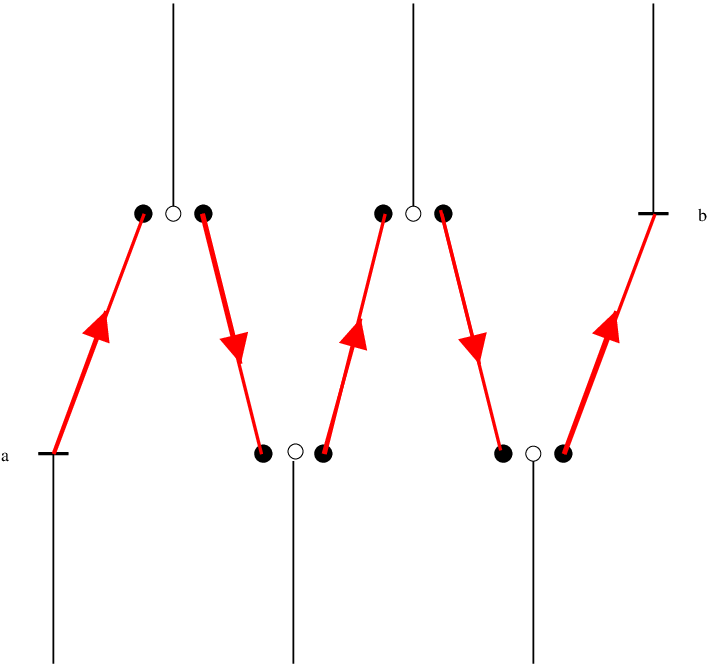
Call this path . We define on the restriction of to by starting at in and then extending out along in the following way. On the segments of joining to , we use the leftmost section when is heading upwards and the rightmost section when is heading downwards. For the turns between and , we use the monotone relation of Lemma 6.18, which associates a point in with , to continue . This then defines the value of at .
In order to construct the universal circle we need to understand how depends on . If is another point in the same , then for any leaf which is incomparable to . Moreover, for in an arbitrary , the two sections and can differ on only part of in the following sense. Let denote the union of with all which are part of the same cataclysm as some . We say that a line is between and if it intersects . Then:
6.22 Lemma.
Suppose and are sections which differ on a leaf . Then lies on a line which lies between and .
Proof.
Suppose that does not lie on a line between and . Then the paths and intersect in a nontrivial subpath ending at . Note that the orientations of and agree on , and that contains at least one turn. The sections and coalesce as they pass through that turn, and so . ∎
On the other hand, we have:
6.23 Lemma.
Let and be two distinct sections, and a line in which lies between . Then and differ on .
Proof.
If and are comparable, then as and are distinct they must differ on the interval in . As the line contains , the two sections differ on . So now assume that and are incomparable.
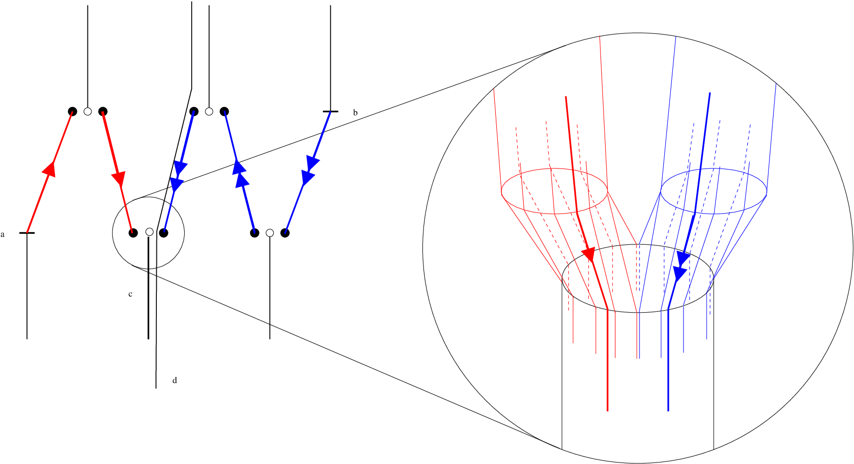
As in Figure 6.24, must pass through a turn of . Thus we have an interval of where the two sections come in via different branches of the cataclysm. So the situation looks like the magnified picture in Figure 6.24. As noted in Remark 6.19, the way the monotone relation works for incomparable leaves implies that the two sections differ on . ∎
Now let denote the set of all special sections . We want to put a natural circular order on by declaring that a triple is clockwise ordered if the restrictions of the to some line are clockwise ordered. To know that this makes sense, we need to check:
6.25 Lemma.
Given three distinct sections , there exists a line so that the restriction of the to has a non-degenerate circular order. Moreover, this circular order is independent of the choice of .
Proof.
Let be the leaf where . The midpoint of the is defined analogously to the midpoint of three points in an -tree. More precisely, we let be the union of the three paths . The midpoint is constructed by making Hausdorff by amalgamating the cataclysms, taking the midpoint in the resulting tree, and then pulling back that midpoint to . The midpoint consists of either a single point in or several points of the same cataclysm. Given Lemma 6.22, if is a leaf where all the differ, then for each pair there is a line containing which intersects . So a natural place to look for the needed line is near the midpoint of the .

There are several cases. First, consider the case where the midpoint is several points of the same cataclysm. There are two subcases corresponding to Figure 6.26(a) and (b). In case (a), the proof of Lemma 6.23 shows that the three sections differ on the interval shown. In case (b), first notice that and differ on the interval . Therefore, differs from at least one of and on . Without loss of generality, assume that . Take to be the line shown in Figure 6.26(c). As is between and , the sections and differ on . As , we know that the are distinct on , and so have a non-degenerate circular order.
In the case that the midpoint is a single point , take any line containing . The midpoint lies in every , and so lies between each pair . By Lemma 6.23, the restricted to are distinct, and so have a non-degenerate circular order.
It remains to prove that the circular order is independent of the choice of the line . Because of Lemma 6.22, this is simple to check in each of the above cases, and we leave this to the reader. ∎
Now that we’ve defined special sections in general and shown they have a circular order, the proof of Theorem 6.2 follows as in the -covered case by completing into a circle. The only difference is that now we need to check Property (4) of Definition 6.1, but this is clear from the construction in Lemma 6.18, and from Remark 6.19 immediately following it.
6.27 Remark.
Note that there is no claim of uniqueness for the universal circles constructed by this or other methods. Even if one asks for minimal universal circles, it is not a priori clear that they should be unique. On the other hand, for -covered foliations or those with one-sided branching, there is a unique minimal universal circle [Cal2, Cal3].
6.28. Faithfulness of the action
Finally, we conclude this section by proving Theorem 6.3, namely that the action of on is faithful provided is atoroidal. If is -covered, then since is atoroidal there is a transverse pseudo-Anosov flow which can be split open to a pair of very full genuine laminations transverse to each other and to . These laminations are covered by genuine laminations which arise from a pair of invariant laminations of . If acts as the identity on , it acts as the identity on the leaf space of either genuine lamination, and therefore it fixes the singular flowlines of the pseudo-Anosov flow (see [Cal2] Corollary 5.3.16); in particular, it acts as a nontrivial translation along these flowlines. But the dynamics of the flow expands the transverse measure on one singular lamination and contracts the transverse measure on the other, and therefore the action on the leaf spaces of the singular foliations is nontrivial, giving a contradiction. So we can assume that the leaf space has branching (in this case, we will not need the assumption that is atoroidal).
Let be the kernel of the map . Let be any leaf of , and a non-identity element in . We claim that and are comparable and distinct. Note that can’t fix setwise, because if it did it would act identically on and hence identically on . If and are incomparable, we know that the maps and blow down different gaps. As acts identically on , this is impossible.
Fix a branch point in . By our above observations, the set is infinite and contained in a line . Now consider a leaf which is in the same cataclysm as . Again, is contained in a line . For each , the leaf is in the same cataclysm as . So there are infinitely many pairs of non-separable points where one point is in and other in . This is not possible for two lines in , and so we have a contradiction. Thus the action on is faithful in the branching case. This completes the proof of Theorem 6.3.
7. Group actions on -manifolds and left orderings
In this section, we discuss the algebraic interdependence between the existence of actions of a group on various -manifolds. The main reason for this is to improve the usefulness of the (non)existence of such a group action as a criterion for the existence of foliations and laminations. In particular, we want to promote an action of on to an action on . This is because it is much easier to decide whether a group admits a a faithful action on than on .
We’ll begin with a more algebraic criterion for a group to act faithfully on . A group is left-orderable if there is a total order on which is invariant under left multiplication. If has a faithful representation into , then is left-orderable for the following reason. Pick an infinite sequence of points such that the intersection of the stabilizers of these points in is trivial. Then say if for the smallest where one of and does not fix , we have . Conversely, for a finitely generated group , it is not hard to show that the existence of a left-invariant order gives rise to a faithful representation in , so these conditions are actually equivalent (see e.g. [Ghys]). For actions on circles, one can use the analogous notion of a circular order to the same effect.
7.1. Lifting representations
Given a group and a representation
when does lift to a representation ? Here we want the lift to respect the universal covering map in the sense that
The topological group has two connected components; the component of the identity is the subgroup of orientation preserving homeomorphisms. If , every homomorphism from to has image in .
There is a universal central extension of
where the group is the group of periodic homeomorphisms of with period ; i.e. those that commute with the translation .
Since is the universal central extension of , the obstruction to lifting a homomorphism is an element of called the Euler class of (for more, see [Ghys]). We will give a geometric interpretation of later, but for the moment we study the implications for where is a rational homology sphere.
7.2 Theorem.
Let be a rational homology sphere and a faithful homomorphism. Then the commutator subgroup is left-orderable.
Proof.
Let . By assumption is finite, so that is torsion. We will show that restricted to lifts to .
For each , there is a lift of to . This lift is not unique, and distinct lifts differ by powers of the generator of the center of . If , we can express as a product of commutators
Consider the element in given by
Since is central, this depends only the description of as a product of commutators, not on the choices of the . We will show that is independent of the choice of expression as a product of commutators. Then will be a homomorphism which is a lift of as required.
If we have another description of as a product of commutators
then the relation
determines a map from a surface , and therefore an element . To see that is well-defined on it suffices to show that
is trivial in . But by the definition of the Euler class, we have that
is zero, because is torsion. So the representation lifts to on , and we are done. ∎
In case of a general action on we have:
7.3 Theorem.
Let be an irreducible rational homology sphere, and
a faithful homomorphism. Let be the kernel of the homomorphism from to defined by the orientation of . Then the subgroup is left-orderable.
Proof.
Consider the manifold corresponding to . If is also a rational homology sphere, then we are done by the preceding theorem. If instead , then itself is left-orderable for reasons that have nothing to do with the existence of , namely the following theorem of from [BRW, Cor. 3.4]:
7.4 Theorem (Boyer, Rolfsen, Wiest).
A compact, orientable, irreducible 3-manifold with has left-orderable fundamental group.
In either case, we’re done. ∎
7.5 Remark.
The necessity of passing to a dihedral cover in general in Theorem 7.3 reflects the fact that finite dihedral groups act faithfully on . For instance, let be a -manifold with a dihedral cover , where , such that is left-orderable. Let have image the standard action of the dihedral group on . The kernel is exactly , and we can modify to a monotonely equivalent faithful action by blowing up the (finite) orbit of some point in , inserting a faithful action of at some blown up interval, and transporting this action around the orbit by .
7.6 Corollary.
Let be an orientable atoroidal -manifold which contains a taut foliation, a tight essential lamination with solid torus guts, or a pseudo-Anosov flow. Then there is a finite cover of with left-orderable fundamental group. The covering group is either an abelian group, or a extension of an abelian group.
7.7. The Euler class and multisections
A more geometric way to think about Euler classes is via foliated bundles and multisections. A representation determines a foliated bundle over , by taking the quotient of the trivial bundle by acting via
Another interpretation of the Euler class of is the obstruction to finding a section of this foliated bundle. For any integer , the class is the obstruction to finding an order multisection of this bundle. The existence of such a multisection gives a representation of on the group of homeomorphisms of copies of , as follows. An order multisection can be parameterized on a small open set by sections . The “labels” on these sections can be analytically continued along a path in , but after traveling around a loop , the labels are permuted by some element in the symmetric group on letters:
Pick a point in , and consider the cover of the fiber by copies of , where the basepoint of the th copy of maps to . As we wind around a loop based at , we can see how much holonomy transport of some leaf twists in relative to the section . But after traveling around the loop, the section gets relabelled as . This holonomy transport gives an identification of the th copy of with the th copy of , and one gets a representation of in the group .
7.8. Flips and canceling Euler classes
Let be a -manifold, and suppose that contains a taut foliation, a tight essential lamination with solid torus guts, or a pseudo-Anosov flow. Then there is a faithful representation . We would like to find a subgroup of , of as large index as possible, where the representation lifts to . From what we have said above, it might seem that the worst case is when . But there are some instances where the nature of these representations helps out, using the flips discussed in Section 3.3.
Suppose is a tight essential lamination of with solid torus guts, and suppose further that there is a homomorphism such that the core of each gut region maps to the identity. Let be the -fold cover corresponding to the kernel of . Then lifts to a tight essential lamination of with two solid torus gut complementary regions for each solid torus gut region of . By the Filling Lemma 4.1, we can assume the complementary regions to were actually ideal polygon bundles over , and the same is therefore true for . The complementary regions to come in pairs corresponding to the complementary regions to . The representation restricts to a representation . If, for each complementary region , we perform a flip of exactly one of the , we get a new representation which is evidently both orientation-preserving and has Euler class . In particular, lifts to a faithful representation in , and is left-orderable. Unfortunately, we see no means of exploiting this trick for algorithmic purposes, since the condition that be trivial on the core of every gut region seems hard to verify in practice.
7.9. Actions on leaf spaces of taut foliations
For completeness, we include a proof of the following fact mentioned in the introduction:
7.10 Theorem.
Let be a taut foliation of . Then admits a faithful action on without a global fixed point.
Proof.
Let be the kernel of the holonomy representation. Then fixes every leaf of . In particular, is a surface group, and is therefore left-orderable, and acts faithfully on . We can insert this action at some point and transport it around by the action of . Geometrically, we can realize such an action by changing the foliation by a monotone equivalence. ∎
7.11 Corollary.
If admits a co-orientable -covered foliation , then is left-orderable.
8. Algorithmic issues
Let be a finitely presented group which has a short-lex automatic structure. In this section, we describe computational techniques for proving that is not left-orderable. The existence of a short-lex automatic structure (see [ECH+] for definitions) implies that the word problem for is efficiently solvable. In fact, there is a set of generators of for which there is a fast algorithm for reducing a word in to the canonical word which is lexicographically first among all shortest words equal to in .
If is orderable, consider the positive cone . Then and is the disjoint union . Conversely, any with these two properties gives rise to a left invariant order via if and only if . Let be the ball in of radius about , that is, all words in of length at most . For fixed , we can consider the following
8.1 Question.
Does there exist a such that and is the disjoint union ?
If is orderable, the answer to (8.1) is yes. If the answer to (8.1) is no, then is not orderable. It is not hard to show that if is non-orderable then the answer to (8.1) is no for large enough . The idea is that if the answer to (8.1) is always yes, then one can construct an global positive cone by taking an inverse limit of the partial positive cones , picking at each stage a which has infinitely many extensions to larger .
For any particular , the automatic structure on combined with the fact that is finite means that (8.1) is algorithmically decidable. We’ll now give a simple recursive algorithm to do this. The algorithm follows a similar line to the proof of Theorem 9.1, and the reader is advised to read that proof before proceeding. Fix and set . The following recursive procedure, constructP, has the property that constructP({ }) returns true if and only if the answer to (8.1) is yes.
| constructP( such that ): | ||
| while : | ||
| if : | ||
| return false | ||
| if : | ||
| return true | ||
| a shortest word in | ||
| return constructP( ) or constructP( ) |
Let’s get a rough grip on how long this algorithm takes in practice. A bad case is when exists as then we have to construct it. Note that even if we’re handed by an oracle, it still takes about multiplications to check that satisfies the conditions in (8.1). If we were to compute a multiplication table for in advance (using multiplications), we could do all further multiplications by table lookup at essentially no cost. So in cases where we end up constructing , we can make the running time and this is roughly the best possible.
However, if the answer to (8.1) is no, in practice one needs far fewer multiplications and only a few () levels of recursion for the algorithm to finish. So in practice, a good strategy seems to be to stop the algorithm if the recursion depth is greater than , and just assume the final answer would have been yes.
The groups we’re interested in are the fundamental groups of hyperbolic 3-manifolds. These do have short-lex automatic structures. The problem is that has exponential growth with . For the 2-generator groups we looked at in Section 10, is usually a little less that . In practice, the size of makes it very difficult to decide (8.1) if is bigger than, say, . Given this, it is remarkable that among the small volume closed hyperbolic 3-manifolds in the Hodgson-Weeks census there are quite a few whose fundamental groups can be shown to be non-orderable by this method (see Section 10).
The algorithm can be easily modified to keep track of the origin of an element of as a product of the elements that have been added to . This lets one generate a proof that the group is non-orderable. In fact, this was how we found the proof of Theorem 9.2.
9. The Weeks manifold
The Weeks manifold is the smallest known hyperbolic 3-manifold. In this section, we will show that its fundamental group cannot act faithfully on or . The Weeks manifold is the Dehn surgery on the Whitehead link (our convention is that surgery on a component of this link yields the trefoil). It is arithmetic, and its volume is about . Its fundamental group is
where and .
We’ll begin with the easy case of actions on .
9.1 Theorem.
The fundamental group of the Weeks manifold is non-orderable.
Proof.
Suppose that is orderable. Consider the positive cone
Then and is the disjoint union . Switching around if necessary, we can assume that , that is . We now consider the various possibilities.
- Case .
As , we have , etc. contained in .
- Subcase .
Then is in . But in , and so , a contradiction.
- Subcase .
Then is in . But in , and so , a contradiction.
- Subcase .
- Case .
Using the relations and we have
in . But then , a contradiction.
This shows that such a does not exist, and so is non-orderable. ∎
Next we’ll show:
9.2 Theorem.
The fundamental group of the Weeks manifold has no faithful action on .
Proof.
Suppose that acts faithfully on a circle. Since , the action is orientation preserving. The Euler class of the action must be nontrivial as the previous theorem shows that can’t action faithfully on . Now , and so has order . By Section 7.7, this means that acts faithfully on the union of lines. Let be the stabilizer of one of the lines. The subgroup acts faithfully on that line and so is left-orderable. The action on the set of lines is transitive, since is the smallest multiple of which vanishes; thus has index in . To prove the theorem, we’ll show that no subgroup of of index is left-orderable.
One can check that the only subgroups of of index are normal. So is normal and . Thus is the kernel of some homomorphism , and there are possibilities for . Consider the automorphisms of given by
(To check that induces an automorphism, use the relation mentioned above.) Together, and generate a subgroup of the outer automorphism group isomorphic to (in fact, this is the whole isometry group of ).
In any event, it is easy to check that under the action of there are two orbits of subgroups of index in . Representatives of these orbits are , the kernel of the homomorphism sending and , and , the kernel of and .
First we’ll show that is non-orderable. Let be the positive cone, and assume that . The proof is completed by considering the following cases. The needed identities in can be checked in number of ways, e.g. by using automatic groups, multiplying matrices, or for the determined, the relations and a chalkboard.
- Case .
Then in P.
- Case .
- Subcase .
Then
- Subcase .
Set . Then
- Subcase .
This completes the proof that is non-orderable.
Now consider . We can assume that . The cases are:
- Case .
Then
- Subcase .
Then
- Subcase .
Then
- Subcase .
- Case .
- Subcase .
Then
- Subcase .
Then
- Subcase .
This proves that is non-orderable. This completes the proof that does not act faithfully on . ∎
In fact, one can show more:
9.3 Theorem.
Let be the fundamental group of the Weeks manifold. Then any homomorphism has image which is either trivial or .
Proof.
Consider a nontrivial action of on the circle. Let be the kernel of . We can apply the proofs of Theorems 9.1 and 9.2 to unless one of the elements we added to is in . In other words, we have a contradiction unless one of
is in . But it is easy to check that the quotient of by the normal closure of any of the above words is . So and we’re done. ∎
As a corollary of these non-existence results, we get the following:
9.4 Corollary.
The Weeks manifold does not admit a taut foliation, a tight essential lamination, or a pseudo-Anosov flow.
Proof.
As the fundamental group of the Weeks manifold can’t act on , the first and last assertions follow immediately from Theorem 6.3 and Corollary 3.9. For tight essential laminations, though, to apply Theorem 3.2 we need the additional hypothesis that the lamination has solid torus guts. So it remains to show:
9.5 Claim.
Let be a tight genuine lamination of the Weeks manifold . Then the complementary regions of have a decomposition where all the gut regions are solid tori.
This will follow from Agol’s work on volumes of 3-manifolds with tight laminations. A decomposition of into interstices and guts has minimal guts if in every complementary region , the interstitial regions are the whole characteristic -bundle of . Such a decomposition is unique up to isotopy. In [Agol], Agol shows:
9.6 Theorem (Agol).
Let be a hyperbolic 3-manifold, and a tight genuine lamination. Let be the guts of the minimal decomposition of . Then
where is the volume of the regular ideal tetrahedron in .
So now let be a gut region of the minimal decomposition of . By Agol’s theorem, we must have as . Thus the boundary of consists of tori. The boundary of is incompressible outward into , and so as is atoroidal, the boundary of is compressible into . Therefore is a solid torus. This proves the claim, and thus the corollary. ∎
10. Further examples
For the smallest manifolds in the Hodgson-Weeks census [W] of closed hyperbolic 3-manifolds we tried to determine which act faithfully on . We looked at the census manifolds of volume which are -homology spheres (so any action would be orientation preserving). There are such manifolds. Using the algorithm of Section 8, we showed that at least of them can’t act faithfully on . Conversely, we showed that at least of them have such actions. We also found that at least have essential laminations. See the table below for details. We would have liked to give more examples where the fundamental group can’t act faithfully on , but the only manifold where we were able to succeed at this was the Weeks manifold.
The algorithm was implemented starting from group presentations generated by SnapPea and using the automatic groups program KBMAG [Holt] to solve the word problem.
To show manifolds contain essential laminations, we used two techniques. The first is that for many simple knots, such as two-bridge knots or most knots under 11 crossings, every nontrivial Dehn surgery contains an essential lamination (see [Gab, pg. 8] and the references therein). In particular, this is true for the knots that appear in the table below. In some cases, such as for two-bridge knots, one can take the lamination to be a taut foliation [Del].
The second technique also uses Dehn filling, but is more complicated to explain. Let be a 3-manifold with torus boundary whose interior is hyperbolic. Gabai and Mosher [Mos] proved that contains a pair of laminations coming from a pseudo-Anosov flow associated to a finite depth foliation. When fibers over , these are just the suspensions of the stable and unstable laminations of the surface homeomorphism. There is a degeneracy slope in associated to with the following property: for any slope with , the laminations remain essential in the Dehn filling (for more see [Mos, Thm. B] or the summary of this theory in [Bri2]).
In general, it is quite difficult to determine the degeneracy slope. Here, we used the following trick. Suppose has Dehn fillings which have finite fundamental group. The don’t contain any essential laminations. Now consider some other filling . If also has no essential lamination, we must have and where is the degeneracy slope. So if there does not exist such a , we can conclude that has an essential lamination. What’s more, that essential lamination in is very full, because the laminations are themselves very full.
Below is the table summarizing our findings. In the Ord column, N means that the fundamental group is non-orderable, O means that it is orderable, and blank means unknown. The Lam column lists an L if the manifold is known to contain an essential lamination. If the manifold is known to contain an essential lamination, the final column gives the reason. In that column, means the complement of the two-bridge knot, and numbers of the form refer to the complements of the corresponding knots in the standard table [Rol]. For the trick with the degeneracy slope, we give the particular expression as a Dehn filling that was used.
Finally, the reason that the indicated manifolds have orderable fundamental group is that they have taut foliations and are integral homology spheres. In such cases, the action on the universal circle lifts to a faithful action on .
| Name | Volume | Hom | Ord | Lam | Reason for knowing laminar |
|---|---|---|---|---|---|
| 0.9427073628 | N | ||||
| 0.9813688289 | L | Is and is . | |||
| 1.2637092387 | N | L | Degeneracy test as . | ||
| 1.3985088842 | O | L | Is and is . | ||
| 1.4236119003 | N | ||||
| 1.4406990067 | L | Is and is . | |||
| 1.4637766449 | L | Is and is . | |||
| 1.5294773294 | L | Is and is . | |||
| 1.5435689115 | N | L | Degeneracy test as . | ||
| 1.5435689115 | N | L | Degeneracy test as . | ||
| 1.5831666606 | N | ||||
| 1.5831666606 | N | ||||
| 1.6496097158 | N | L | Degeneracy test as . | ||
| 1.7571260292 | L | Is and is . | |||
| 1.8243443222 | N | L | Degeneracy test as . | ||
| 1.8854147256 | N | L | Degeneracy test as . | ||
| 1.8854147256 | N | L | Degeneracy test as . | ||
| 1.8859142560 | N | L | Degeneracy test as . | ||
| 1.9122102501 | L | Is and is . | |||
| 1.9222971095 | N | ||||
| 1.9537083154 | N | L | Degeneracy test as . | ||
| 1.9627376578 | N | L | Degeneracy test as . | ||
| 1.9627376578 | N | ||||
| 2.0143365838 | |||||
| 2.0259452819 | N | ||||
| 2.0288530915 | L | Is and is . | |||
| 2.0298832128 | |||||
| 2.0555467489 | |||||
| 2.0656708385 | L | Is and is . | |||
| 2.1030952907 | L | Is and is . | |||
| 2.1145676931 | N | L | Degeneracy test as . | ||
| 2.1145676931 | L | Is and is . | |||
| 2.1243017573 | |||||
| 2.1557385676 | N | ||||
| 2.1557385676 | N | L | Degeneracy test as . | ||
| 2.1847555751 | L | Is and is . | |||
| 2.1959641187 | N | ||||
| 2.2082823597 | N | L | Degeneracy test as . | ||
| 2.2102443409 | L | Degeneracy test as . | |||
| 2.2109517391 | L | Degeneracy test as . | |||
| 2.2267179039 | O | L | Is and is . | ||
| 2.2267179039 | L | Is and is . | |||
| 2.2597671326 | L | Is and is . | |||
| 2.2662435733 | L | Is and is . | |||
| 2.2726318636 | |||||
| 2.2757758101 | N | L | Degeneracy test as . | ||
| 2.2944383001 | L | Is and is . | |||
| 2.3126354033 | |||||
| 2.3188118677 | N | L | Degeneracy test as . | ||
| 2.3188118677 | |||||
| 2.3207602675 | L | Is and is . | |||
| 2.3380401178 | N | ||||
| 2.3522069054 | N | L | Degeneracy test as . | ||
| 2.3522069054 | N | ||||
| 2.3641969332 | N | L | Degeneracy test as . | ||
| 2.3705924006 | |||||
| 2.3803358221 | N | L | Degeneracy test as . | ||
| 2.4224625169 | L | Is and is . | |||
| 2.4444077795 | L | Degeneracy test as . | |||
| 2.4540294422 | |||||
| 2.4631393944 | |||||
| 2.4682321967 | N | ||||
| 2.4682321967 | N | L | Degeneracy test as . | ||
| 2.4878225918 | N | ||||
| 2.4903791858 | |||||
| 2.5026593054 | L | Is and is . | |||
| 2.5065758445 | N | ||||
| 2.5144043349 | |||||
| 2.5274184773 | L | Degeneracy test as . | |||
| 2.5274184773 | |||||
| 2.5274184773 | |||||
| 2.5303032876 | N | ||||
| 2.5415850101 | |||||
| 2.5495466001 | |||||
| 2.5667347900 | |||||
| 2.5689706009 | |||||
| 2.5751620736 | |||||
| 2.5854830480 | L | Degeneracy test as . | |||
| 2.5953875937 | N | ||||
| 2.6095439552 | |||||
| 2.6122234482 | |||||
| 2.6172815707 | L | Degeneracy test as . | |||
| 2.6244624283 | N | ||||
| 2.6285738915 | L | Is and is . | |||
| 2.6294053953 | O | L | Is and is . | ||
| 2.6414714456 | L | Degeneracy test as . | |||
| 2.6536080625 | L | Degeneracy test as . | |||
| 2.6555425236 | |||||
| 2.6646126469 | L | Degeneracy test as . | |||
| 2.6735274161 | L | Is and is . | |||
| 2.6822267321 | L | Is and is . | |||
| 2.6954841673 | N | L | Degeneracy test as . | ||
| 2.6954841673 | |||||
| 2.7067833105 | N | L | Is Haken. See [Dun]. | ||
| 2.7124588084 | L | Is and is . | |||
| 2.7589634387 | L | Is and is . | |||
| 2.7725163132 | N | ||||
| 2.8022537823 | |||||
| 2.8281220883 | |||||
| 2.8281220883 | |||||
| 2.8281220883 | |||||
| 2.8458961160 | N | ||||
| 2.8472238006 | N | ||||
| 2.8472238006 | |||||
| 2.8656302333 | |||||
| 2.8669017766 | N | L | Degeneracy test as . | ||
| 2.8669017766 | L | Degeneracy test as . | |||
| 2.8733431176 | |||||
| 2.8733431176 | |||||
| 2.8824943873 | Is Haken. See [Dun]. | ||||
| 2.9027039980 | L | Degeneracy test as . | |||
| 2.9133321143 | |||||
| 2.9169341134 | |||||
| 2.9356518985 | |||||
| 2.9398104423 | |||||
| 2.9400386172 | N | ||||
| 2.9438596478 | |||||
| 2.9545326040 | |||||
| 2.9582502906 | |||||
| 2.9605565159 | N | ||||
| 2.9607151670 | |||||
| 2.9670703390 | |||||
| 2.9696321386 | |||||
| 2.9709840073 | L | Degeneracy test as . | |||
| 2.9760925194 | |||||
| 2.9769925267 | L | Is and is . | |||
| 2.9781624873 | |||||
| 2.9868370451 |
References
- [Agol] I. Agol. Lower bounds on volumes of hyperbolic Haken 3-manifolds, preprint, 1999. arXiv:math.GT/9906182.
- [BRW] S. Boyer, D. Rolfsen, and B. Wiest. Orderable 3-manifold groups. Preprint, 2002.
- [Bri1] M. Brittenham. Essential laminations in non-Haken -manifolds. Topology Appl. 53 (1993), 317–324.
- [Bri2] M. Brittenham. Essential laminations, exceptional Seifert-fibered spaces, and Dehn filling. J. Knot Theory Ramifications 7 (1998), 425–432.
- [Cal1] D. Calegari. Foliations and the Geometry of 3-manifolds. PhD thesis, U.C. Berkeley, 2000.
- [Cal2] D. Calegari. The geometry of -covered foliations. Geom. Topol. 4 (2000), 457–515.
- [Cal3] D. Calegari. Taut foliations with one-sided branching. Geom. Dedicata (to appear).
- [Can1] A. Candel. Uniformization of surface laminations. Ann. Sci. École Norm. Sup. (4) 26 (1993), 489–516.
- [Can2] A. Candel. The harmonic measures of Lucy Garnett. Preprint.
- [Del] C. Delman. Essential laminations and Dehn surgery on -bridge knots. Topology Appl. 63 (1995), 201–221.
- [Dun] N. M. Dunfield. Which small volume hyperbolic 3-manifolds are Haken? Slides from a talk at the University of Warick, 1999, availible at http://www.math.harvard.edu/~nathand.
- [ECH+] D. B. A. Epstein, J. W. Cannon, D. F. Holt, S. V. F. Levy, M. S. Paterson, and W. P. Thurston. Word processing in groups. Jones and Bartlett Publishers, Boston, MA, 1992.
- [FM] B. Farb and L. Mosher. A rigidity theorem for the solvable Baumslag-Solitar groups. Invent. Math. 131 (1998), 419–451. With an appendix by Daryl Cooper.
- [Fen] S. R. Fenley. The structure of branching in Anosov flows of -manifolds. Comment. Math. Helv. 73 (1998), 259–297.
- [Gab] D. Gabai. Problems in foliations and laminations. In W. H. Kazez, editor, Geometric Topology, Proceedings of the 1993 Georgia International Topology Conference, pages xiv+473, Providence, RI, 1997. American Mathematical Society.
- [GK1] D. Gabai and W. H. Kazez. Homotopy, isotopy and genuine laminations of -manifolds. In Geometric topology (Athens, GA, 1993), pages 123–138. Amer. Math. Soc., Providence, RI, 1997.
- [GK2] D. Gabai and W. H. Kazez. Order trees and laminations of the plane. Math. Res. Lett. 4 (1997), 603–616.
- [GK3] D. Gabai and W. H. Kazez. Group negative curvature for -manifolds with genuine laminations. Geom. Topol. 2 (1998), 65–77.
- [GO] D. Gabai and U. Oertel. Essential laminations in -manifolds. Ann. of Math. (2) 130 (1989), 41–73.
- [Gar] L. Garnett. Foliations, the ergodic theorem and Brownian motion. J. Funct. Anal. 51 (1983), 285–311.
- [Ghys] É. Ghys. Groups acting on the circle. Enseign. Math. (2) 47 (2001), 329–407.
- [Holt] D. Holt. KBMAG2: Knuth-Bendix in Monoids, and Automatic Groups. 2.4 (1999). http://www.maths.warwick.ac.uk/~dfh/.
- [Mos] L. Mosher. Laminations and flows transverse to finite depth foliations, Part I: Branched surfaces and dynamics. Preprint, 1996.
- [Pla] J. F. Plante. Foliations with measure preserving holonomy. Ann. of Math. (2) 102 (1975), 327–361.
- [RSS] R. Roberts, J. Shareshian, and M. Stein. Infinitely many hyperbolic 3-manifolds which contain no Reebless foliation. Preprint, 2001.
- [Rol] D. Rolfsen. Knots and links. Publish or Perish Inc., Berkeley, Calif., 1976. Mathematics Lecture Series, No. 7.
- [Tar] V. M. Tararin. On automorphism groups of cyclically ordered sets. Sibirsk. Mat. Zh. 42 (2001), 212–230, iv.
- [Thu] W. P. Thurston. Three-manifolds, Foliations and Circles, II. Unfinished manuscript, 1998.
- [W] J. Weeks. SnapPea. http://www.northnet.org/weeks/.
- [Wit] D. Witte. Arithmetic groups of higher -rank cannot act on -manifolds. Proc. Amer. Math. Soc. 122 (1994), 333–340.