Invariants of tangles with flat connections in their complements.I. Invariants and holonomy $R$-matrices

Let $I\equiv[0,1]$ be the unit closed interval. A geometric tangle $t\subset{{\mathbb{R}}^{2}}\times I$ is the image of an embedding

with oriented components such that

and $\partial t\cap{{\mathbb{R}}^{2}}\times\partial I=t\cap{{\mathbb{R}}^{2}}\times\partial I$.

Let $(x,y,z)$, $x,y\in{\mathbb{R}}$, $z\in I$, be Cartesian coordinates on ${{\mathbb{R}}^{2}}\times I$. Denote by $D_{t}$ the image of $t$ under the projection

We call geometric tangle $t$ restricted if it is based on lines $L_{\pm}=\{(0,y,(1\pm 1)/2)\}$, i.e. $\partial t\in L_{+}\cup L_{-}$. Denote by

the boundary components of $t$ and $D_{t}$ which belong to $L_{\pm}$ and their images in $D_{t}$, respectively.

Projection $D_{t}$ is called regular if it has only double points at which segments intersect transversely, all critical points in $z$-direction are non-degenerate, and non of the critical points coincide with any of the double points. A regular projection $D_{t}$ will be called diagram of $t$. The vertices of a diagram are its double points, critical points in $z$-direction and boundary points, while edges are the segments running between the vertices. A vertex of $D_{t}$ is called positive or $(+)$ crossing if it is a double point and the angle between lower and upper components is positive. If the angle is negative, the vertex is called negative or $(-)$ crossing, see Fig. 1.

For each double point $v$ of diagram $D_{t}$ denote by $a_{v},b_{v},c_{v},d_{v}$ the adjacent edges in accordance with Fig. 2, and for each critical point $v$ denote by $l_{v},r_{v}$ the adjacent edges as in Fig. 3.

Define group $\Pi(D_{t})$ generated by edges of $D_{t}$ with the following defining relations:

• •

  for each double point $v$

  $$\begin{array}[]{rl}(+)\mbox{ crossing:}&a_{v}=d_{v},\ b_{v}=d_{v}^{-1}c_{v}d_{v}\\ (-)\mbox{ crossing:}&b_{v}=c_{v},\ a_{v}=c_{v}d_{v}c_{v}^{-1}\end{array}$$

• •

  for each critical point $v$: $l_{v}r_{v}=1$.

The isomorphism class of this group does not depend on the diagram representing $t$ and is isomorphic to the fundamental group of the complement to $t$:

In fact, the definition of $\Pi(D_{t})$ concides with the Wirtinger presentation of $\pi_{1}({\mathbb{R}}^{2}\times I\backslash t)$. One can fix an isomorphism by choosing a base point $x_{0}$ in ${\mathbb{R}}^{2}\times I\backslash t$ and associating to each edge $e$ in $D_{t}$ element $\Gamma^{x_{0}}_{e}$ of $\pi_{1}({\mathbb{R}}^{2}\times I\backslash t,x_{0})$ which is represented by the loop at $x_{0}$ with projection as in Fig. 4. We shall call such correspondence a monodromy map.

Associated with boundary of $D_{t}$, group $\Pi(D_{t})$ has two natural subgroups $\Pi(\partial_{\pm}D_{t})$ generated by edges intersecting with corresponding boundary components. One has the following commutative diagram:

where the hookarrows are embeddings while the arrows are natural group homomorphisms, and we denote $x^{\pm}_{0}=(x,y,(1\pm 1)/2)$ the projections of the base point $x_{0}=(x,y,z)$. The base point is chosen such that it projects to the plane of the diagram $D_{t}$ to the far left of it (in the $y$-direction).

For a Lie group $G$ let $A$ be the 1-form corresponding to a flat connection in a principle $G$-bundle over the complement to tangle $t$ in ${\mathbb{R}}^{2}\times I$. Such form defines a group homomorphism $\pi_{1}({\mathbb{R}}^{2}\times I\backslash t,x_{0})\to G$ which maps the element generated by path $\Gamma$ to the holonomy of $A$ along $\Gamma$. Because we have the isomorphism $\pi_{1}({\mathbb{R}}^{2}\times I\backslash t,x_{0})\simeq\Pi(D_{t})$ a flat $G$-connection also defines a group homomorphism

We denote the space of all such homomorphisms as $\Pi(D_{t},G)$. The group $G$ acts on $\Pi(D_{t},G)$ by conjugations

In terms of $\pi_{1}({\mathbb{R}}^{2}\times I\backslash t,x_{0})\simeq\Pi(D_{t})$ this action corresponds to the changes of the trivialization of the $G$-bundle at the base point, i.e. to gauge transformations.

Thus, the gauge class of the flat connection $A$ defines an element in the coset space $\Pi(D_{t},G)/G$. This gives a combinatorial description of the space of isomorphism classes of representations of the fundamental group of ${\mathbb{R}}^{2}\times I\backslash t$ in $G$ ( or equivalently, of the modulai space of flat connections):

Notice that this description of the isomorphism classes of representations of the fundamental group works also in cases when $G$ is not a Lie group.

Notice that the homomorphism $f:\pi_{1}({\mathbb{R}}^{2}\times I\backslash,x_{0})\to G$ does not define a flat connection in the complement of the tangle. It only defines a gauge class of a flat connection.

For what will follow we need slightly more then a representation of the fundamental group, but less then a flat connection. Let $\tilde{x}_{0}$ be a point which projects to the far right from $D_{t}$. A pair $(f,g)$ where $f$ is a representation of the fundamental group and $g\in G$ is called a ramified representation of the fundamental group if $g$ has a meaning of the holonomy of a flat connection whose gauge class is defined by $f$ along the path connection $x_{0}$ and $\tilde{x}_{0}$ in such a way that it projects ”over” the diagram $D_{t}$ (see Fig. 5).

Let $\{g_{e}\}_{e\in E(D_{t}},g_{r}$ be a ramified representation of the fundamental group. The gauge group acts on it as $g_{e}\mapsto gg_{e}g^{-1},\ g_{r}\mapsto gg_{r}h^{-1}$. Thus the action of the gauge group on ramified representations reduces to the action of $G\times G$. The isomorphism class does not depend on the ramification.

We say that group $G$ is factorizable into two subgroups $G_{\pm}\subset G$ if any element $g\in G$ can be represented in a unique way as

where $g_{\pm},\bar{g}_{\pm}\in G_{\pm}$.

Let $G$ be a Lie group with Lie algebra $\mathfrak{g}$. We say that Lie algebra $\mathfrak{g}$ is factorizable into two Lie subalgebras $\mathfrak{g}_{\pm}$ if for each $x\in\mathfrak{g}$ there exists unique pair $x_{\pm}\in\mathfrak{g}_{\pm}$ such that

A Lie group with factorizable Lie algebra is almost factorizable (i.e. factorizable on an open dense subset). It will be called factorizable Lie group. We will be especially interested in the case when $G$ is an algebraic Lie group with factorizable Lie algebra. Then it is factorizable on a Zariski open subset of $G$.

Another important case is the conditional factorization. In conditionally factorizable Lie algebras factorization (2) is unique only under extra conditions on $x_{\pm}$. For example, fixing a Borel subalgebra ${\mathfrak{b}}_{+}$ in a simple Lie algebra $\mathfrak{g}$ makes $\mathfrak{g}$ conditionally factorizable with ${\mathfrak{g}}_{\pm}={\mathfrak{b}}_{\pm}$ and with the condition $x_{+}|_{\mathfrak{h}}=-x_{-}|_{\mathfrak{h}}$, where ${\mathfrak{h}}$ is the corresponding Cartan subalgebra.

Let $G$ be a factorizable group. Define a binary operation

which obviously defines a group structure on $G$ with the same identity element as for the original group structure. The inverse to $g$ in this group is $i(g)=g_{+}^{-1}g_{-}$. For factorizable Lie groups this structure is defined on a dense open subset of $G$ (or on $G_{+}\times G_{-}$).

Assume $G$ is a factorizable group and $D_{t}$ is a regular diagram of a tangle.

For factorizable $G$ we will make the standard choice of ramification of a representation of the fundamental group of the complement. Assume that the representation is generic and that $\{x_{e}\}$ is the $G$-coloring corresponding to it. Then the standard ramification is obtained by applying rules from Fig. 6 to the path ramification path connection points $x_{0}$ and $\tilde{x}_{0}$:

Here $e_{1},\dots,e_{n}$ are edges of $D_{t}$ which intersect with the ramification path.

Restricted geometric tangle $t$ is called standard if $\partial_{\pm}t=\{(0,1,1),(0,2,1)\dots(0,n_{\pm},1)\}$ for some $n_{\pm}\in{\mathbb{Z}}_{\geq 0}$. We identify planes ${\mathbb{R}}^{2}\times\{0\}$ and ${\mathbb{R}}^{2}\times\{1\}$ with ${\mathbb{R}}^{2}$ through the projection $p$ defined in  (1).

Consider the set of pairs $(t,f,g)$, where $t$ is a standard tangle and $f:\pi_{1}({\mathbb{R}}^{2}\times I\backslash t,x_{0})\to G$ is a group homomorphism and $g\in G$ is its ramification. Define the following equivalence relation on this set. Pair $(t,f,g)$ is equivalent to $(t^{\prime},f^{\prime},g)$ if $t$ is isotopic to $t^{\prime}$ in ${{\mathbb{R}}^{2}}\times I$ by an isotopy preserving the boundary and points $x_{0},\ \tilde{x}_{0}$ (so, in particular, $\partial_{\pm}t=\partial_{\pm}t^{\prime}$), which brings flat connection $f$ to $f^{\prime}$. Equivalence class $[t,f,g]$ will be called a (standard) tangle with a ramified representation of the fundamental group in the complement.

From now on the point $x_{0}$ will have coordinates $(0,y_{0},1/2)$ with $y_{0}<<-1$ and $\tilde{x}_{0}$ will have coordinates $(0,\tilde{y}_{0},1/2)$ with $\tilde{y}_{0}>>1$.

Let $t_{1}$ and $t_{2}$ be two standard geometrical tangles with $\partial_{+}t_{1}=\partial_{-}t_{2}$. Define their composition $t_{1}\circ t_{2}$ as the tangle with the following defining properties:

Here the identifications are given by linear maps, $(x,y,z)\to(x,y,2z)$ for the first one, and $(x,y,z)\to(x,y,2z-1)$ for the second.

Let $[t_{1},f_{1},g]$ and $[t_{2},f_{2},g]$ be two tangles with flat connection in their complements such that $\partial_{+}t_{1}=\partial_{-}t_{2}$ and $f_{1}\big|_{\pi_{1}({{\mathbb{R}}^{2}}\backslash\partial_{+}t_{1},p(x_{0}))}=f_{2}\big|_{\pi_{1}({{\mathbb{R}}^{2}}\backslash\partial_{-}t_{2},p(x_{0}))}$ and $f_{1}$ and $f_{2}$ have the same ramifications. Define the mapping $f_{1\circ 2}$

where we identified elements of fundamental groups using (4) and (5). The map $f_{1\circ 2}$ is a representation of the fundamental group of the complement of $t_{1}\circ t_{2}$. We define the composition of two tangles with flat connections $[t_{1},f_{1},g]$ and $[t_{2},f_{2},g]$ as the equivalence class $[t_{1}\circ t_{2},f_{1\circ 2},g]$ and denote it as $[t_{1},f_{1},g]\circ[t_{2},f_{2},g]$. It is clear that the composition of two tangles with flat connections defined this way does not depend on the choice of representatives in $[t_{1},f_{1},g]$, $[t_{2},f_{2},g]$, and it is associative.

Let $[t_{1}]$ and $[t_{2}]$ be isotopy classes of two standard tangles. Let $|X|$ be the cardinality of a finite set $X$. Consider the map $\varphi:{\mathbb{R}}^{2}\times I\to{\mathbb{R}}^{2}\times I$ acting at the boundary as

Let $x_{0}(i)$ and $\tilde{x}_{0}(i)$ be the reference points for $t_{i}$ ($i=1,2$). Assume that the map $\varphi$ brings a representative $t_{2}$ of $[t_{2}]$ to $t^{\prime}_{2}$ and that it brings $x_{0}(2)$ to $\tilde{x}_{0}(1)$. Choose representatives of $t_{1}$ and $t_{2}$ in such a way that one dimensional submanifolds $t_{1}$ and $t^{\prime}_{2}$ do not tangle with each other ( that their diagrams do not intersect). The isotopy class of $t_{1}\cup t^{\prime}_{2}$ is called the tensor product $[t_{1}]\otimes[t_{2}]$ of $[t_{1}]$ and $[t_{2}]$ [T-1]. It is clear that $[t_{1}]\otimes[t_{2}]$ does not depend on the choice of representatives.

Let $[t_{1},f_{1}]$ and $[t_{2},f_{2}]$ be two tangles with given representations of the fundamental group of the complement. Let $t_{1}$ and $t^{\prime}_{2}$ be geometrical tangles as above. It is clear that $\pi_{1}({\mathbb{R}}^{2}\times I\backslash t_{1}\cup t^{\prime}_{2},x_{0}(1))$ is isomorphic to the group freely generated by $\pi_{1}({\mathbb{R}}^{2}\times I\backslash t_{1},x_{0}(1))$ and $\pi_{1}({\mathbb{R}}^{2}\times I\backslash t^{\prime}_{2},x_{0}(2))$. Definition of the tensor product will depend on how we embed groups $\pi_{1}({\mathbb{R}}^{2}\times I\backslash t_{i},x_{0}(i))$ into $\pi_{1}({\mathbb{R}}^{2}\times I\backslash t_{1}\cup t^{\prime}_{2},x_{0}(1))$.

Fix an isomorphism by identifying elements of $\pi_{1}({\mathbb{R}}^{2}\times I\backslash t_{1}\cup t^{\prime}_{2},x_{0}(1))$ with corresponding elements of $\pi_{1}({\mathbb{R}}^{2}\times I\backslash t_{1},x_{0}(1))$ and $\pi_{1}({\mathbb{R}}^{2}\times I\backslash t^{\prime}_{2},x_{0}(2))$ in accordance with Fig. 7. This identification means that we identify elements of $\pi_{1}({\mathbb{R}}^{2}\times I\backslash t^{\prime}_{2},x_{0}(2))$ with elements of $\pi_{1}({\mathbb{R}}^{2}\times I\backslash t_{1}\cup t^{\prime}_{2},x_{0}(1))$ by gluing them with the ramification path for $t_{1}$.

For a pair of group ramified homomorphisms $f_{i}:\pi_{1}({\mathbb{R}}^{2}\times I\backslash t_{i},x_{0})\to G$, $i=1,2$, with ramifications $g_{1}$ and $g_{2}$ respectively define the group homomorphism

by assigning

The ramification of $f_{1\otimes 2}$ we will define as $g_{1}g_{2}\in G$. The equivalence class of $(t_{1}\cup t^{\prime}_{2},f_{1\otimes 2})$ will be called the tensor product of $[t_{1},f_{1},g_{1}]$ and $[t_{2},f_{2},g_{2}]$ and will be denoted $[t_{1},f_{1},g_{1}]\otimes[t_{2},f_{2},g_{2}]$. This operation is associative.

A framing of a geometric tangle $t$ is a continuous nonsingular section of the normal bundle to $t$. A framing of a tangle is the homotopy class of a geometric framing. We assume that the framing is parallel to the $x$-axis at $\partial_{\pm}t$, has positive projection to this axis and unit length.

Here $G$-framed tangle is a tangle with a ramified representation of the fundamental group of the complement.

Define the category of framed $G$-tangles $\widetilde{\mathcal{F}T}(G)$ as follows:

• •

  Objects are pairs $(\emptyset;f)$ where $f:\pi_{1}({\mathbb{R}}^{2})\to e\in G$ with the trivial ramification ($g=1$) and $((\epsilon_{1},\dots,\epsilon_{n});f,g)$ where $\epsilon_{i}=\pm 1$, $f$ is a representation of the fundamental group of ${{\mathbb{R}}^{2}}\backslash\{(0,1),\dots,(0,n)\}$ with the ramification $g$.

• •

  Morphisms between $((\epsilon_{1},\dots,\epsilon_{n});f_{+};g_{+})$ and $((\sigma_{1},\dots,\sigma_{k});f_{-};g_{-})$ are nontrivial only if $g_{+}=g_{-}$. They are oriented framed tangles with flat connections (with ramified representation of the fundamental group of the complement) $[t,f,g]$ where $t$ is a tangle with $|\partial_{-}t|=k$, $|\partial_{+}t|=n$ and $f$ is a flat connection in the complement of $t$ such that $f|_{\pi_{1}({\mathbb{R}}^{2}\backslash\partial_{\pm}t,x_{0})}=f_{\pm}$. The ramification $g$ is defined by the ramifications of the objects $g=g_{+}=g_{-}$. The orientation of boundary components should agree with signs $\epsilon_{i},\sigma_{j}$ as is shown on Fig. 8.

  

• •

  The composition is defined above in Subsection 3.2.

• •

  The identity element in End$((\epsilon_{1},\dots,\epsilon_{n}),f,g)$ consists of the identity tangle (see Fig. 9) with the representation of the fundamental group and the ramification uniquely defined by its values on the boundary.

The category $\widetilde{\mathcal{F}T}(G)$ is braided monoidal with the tensor product described above.

The braiding is given by the tangle corresponding to the diagram from Fig. 10. The corresponding ramified representation of the fundamental group of its complement is completely determined by the boundary values which are fixed by the choice of objects.

The category $\widetilde{\mathcal{F}T}(G)$ can be described in terms of equivalence classes of diagrams with elements of $G$ assigned to edges of the diagram.

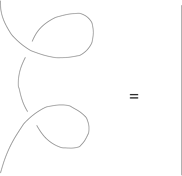
Representations of the fundamental group of the complement to a tangle are in bijections with maps $E(D_{t})\to G$ which satisfy Wirtinger relations. Therefore a tangle with a flat connection in the complement can be regarded as an equivalence class of diagrams equipped with such data modulo Redemeister moves. If the tangle is framed, one has to consider only framed Reidemeister moves (see Figures 11, 12 13).

A representation of the fundamental group of the complement to $n$ distinct points in ${\mathbb{R}}^{2}$ is fixed uniquely by the monodromies along a system of fundamental cycles. Choose them as on Fig. 14 then an object of the category $\widetilde{\mathcal{F}T}(G)$ can be written as a collection $(\epsilon_{1},\dots,\epsilon_{n};\ g_{1},\dots,g_{n};\ g)$ where $g_{i}\in G$ is a monodromy along the cycle shown on Fig. 14 around the point $(0,i,0)$ and $g$ is the ramification.

Thus, we can describe the category $\widetilde{\mathcal{F}T}(G)$ as follows:

• •

  Objects are collections $(\epsilon_{1},\dots,\epsilon_{n};g_{1},\dots,g_{n};g)$, where $\epsilon_{i}=\pm$ and $g_{i},g\in G$.

• •

  Morphisms between the object $(\epsilon_{1},\dots,\epsilon_{n};g_{1},\dots,g_{n};g)$ and the object $(\sigma_{1},\dots,\sigma_{m};h_{1},\dots,h_{m};g)\}$ are diagrams of oriented framed tangles with elements of $G$ assigned to edges modulo Redemeister moves and Wirtinger relations. The orientation and group elements assigned to boundary components should agree the orientation and group elements of corresponding boundary components.

• •

  Composition is the usual composition of diagrams of tangles with group elements assigned to edges.

• •

  Tensor product for objects is $(\{\epsilon_{i}\};\{g_{i}\};g)\otimes(\{\sigma_{i}\};\{h_{i}\};h)=(\{\epsilon_{i}\}\{\sigma_{i}\};\{g_{i}\}\{h_{i}\};gh)$. The tensor product of two morphisms $(D_{1},\{g_{e}\},g)$ and $(D_{2},\{h_{e}\},h$ is the diagram which $D_{1}\sqcup D_{2}$ is the tensor product of two diagrams (juxtaposition) with the elements $g_{e}$ assigned to the edges of $D_{1}$ and elements $g^{-1}h_{e}g$ assigned to edges of $D_{2}$. The ramification of the tensor product is $gh$.

Let $G$ be a factorizable group. According to Theorem 1 a $G$-coloring of diagram $D_{t}$ is in one to one correspondence with a flat $G$-connection in the complement to tangle $t$ by assigning monodromies $\gamma_{e}$ to edges of the diagram:

More precisely, it is a bijection for factorizable groups and a bijection on an open dense subset of $G^{\times E(D_{t})}$ for almost factorizable Lie groups. This suggests the description of the the category $\widetilde{\mathcal{F}T}(G)$ in term of $G$-colored diagrams.

Define the category ${\mathcal{F}T}(G)$ of $G$-colored framed diagrams as follows:

• •

  Objects are sequences $\{(\epsilon_{1},x_{1}),\dots,(\epsilon_{n},x_{n})\}$ where $\varepsilon_{i}=\pm 1$ and generic $x_{i}\in G$.

• •

  Morphisms are $G$-colored framed diagrams modulo framed Reidemeister moves (see Figures 11, 12, 13)

This category is monoidal, braided. The composition is obvious. The tensor product is essentially the same as the tensor product of diagrams of framed tangles (see for example [T-1]). The decoration of the tensor product is defined by the decoration of factors.

Let $\widetilde{\mathcal{F}T}$ be the category of tangles with flat connections in the complement with the standard ramification (see section 2.4).

The proof follows from the bijection between tangles with given representation of the fundamental group of the complement and the equivalence classes of $G$-colored diagrams.

Because the categories $\widetilde{\mathcal{F}T}(G)$and ${\mathcal{F}T}(G)$ are naturally equivalent we will abuse notations and will denote both of them by ${\mathcal{F}T}(G)$.

When $G$ is an almost factorizable Lie group the category of $G$-colored diagrams has the tensor product, but the dual object exists only on an open dense subset of objects. The braiding in this case also exists only on an open subset of objects of this category.

The following fact is a key for construction of invariants of tangles via braided monoidal categories.

The proof of this proposition and the definition of elementary diagrams are the same as for the category of framed tangles (see [T-1]).

Assume we have the following data:

• •

  Collection of finite-dimensional vector spaces ${\mathfrak{X}}$

• •

  For each pair $(X,Y)$ of vector spaces from this collection we have a map

  $$R^{X,Y}:G\times G\to End(X\otimes Y)$$

  (7)

  (or, more generally, a section of a vector bundle over $G\times G$ with the fiber $X\otimes Y$).

Let $x_{L},x_{R}:G\times G\to G$ be mappings acting as

We will call the equation (9) the holonomy Yang-Baxter equation.

For a liner operator $f:V\to V$ we denote by $f^{t}$ the dual linear operator $f^{t}:V^{*}\to V^{*}$.

For cross-nondegenerate holonomy $R$-matrix acting in $X\otimes X$ define the map ( more generally a section of the trivial vector bundle) $d^{X}:G\to End(X)$.

Here and below we will use the notation $t_{i}$ for taking dual to an operator acting in a tensor product with respect to the $i$-th factor.

For $X\in\mathfrak{X}$ and generic $x\in G$ define the linear operator $w_{X}(x)\in End(X)$ as

where $b=i(x^{-1})$.

The proof of this proposition and of the lemma are very similar. Each of the equalities follows from a sequence of equalities where each one corresponds to an elementary moves of corresponding diagrams. They are completely parallel to the proofs of similar statements from [R-1] ( see Fig. 8, Fig. 13-17 from that paper and corresponding sequences of equalities). The only difference is that $G$-coloring should be taken into account.

Let $(D,\{x_{e}\}_{e\in E(D_{t})})$ be a $G$-colored diagram of a tangle. We will call it decorated by vector spaces $\mathfrak{X}$ if a vector space from $\mathfrak{X}$ is assigned to each connected component of the corresponding tangle.

Define the category ${\mathcal{F}C}(G,{\mathfrak{X}})$ of $\mathfrak{X}$-decorated $G$-colored diagrams as follows.

• •

  Objects of ${\mathcal{F}C}(G,{\mathfrak{X}})$ are sequences $\{(\varepsilon_{1},g_{1},X_{1}),\dots(\varepsilon_{n},g_{n},X_{n})\}$ where $\varepsilon_{i}=\pm 1$, $g_{i}\in G^{\prime}\subset G$ (recall that $G^{\prime}\subset G$ is the set of elements in $G$ which admit left and right factorization) and $X_{a}\in{\mathfrak{X}}$.

• •

  Morphisms between two objects $\{(\varepsilon_{a},g_{a},X_{a})\}_{a=1}^{n}$ and $\{(\sigma_{a},h_{a},Y_{a})\}_{a=1}^{k}$ are $G$-colored diagrams decorated by vector spaces from $\mathfrak{X}$ modulo framed Redemeiseter moves. Decorations of boundary components are determined by the initial and the target object. Elements $g_{a}$ and $h_{a}$ are colorings of boundary edges of such diagrams.

• •

  Composition of morphisms is defined by gluing decorated diagrams along the common boundary.

It is clear that $Ad_{G}$ of the $G$-coloring of a morphism in this category can be naturally identified with a gauge class of a flat connections in the complement to the corresponding tangle with connected components colored by $\mathfrak{X}$. The category ${\mathcal{F}T}(G,{\mathfrak{X}})$ is braided monoidal. The tensor product and the braiding are essentially the same as in the category ${\mathcal{F}T}(G)$.

Here we will show how to use a system of holonomy $R$-matrices to construct invariants of tangles with flat $G$-connections in the complement. The construction is similar to the one of invariants of tangles given in [RT]. We will construct the monoidal functor from the category $\tilde{{\mathcal{F}}C}(G,{\mathfrak{X}})$ to the category of all vector spaces.

References

- [J] V. Jones A new knot polynomial and von Neumann algebras. Bull.Amer.Math.Soc.(N.S.)12(1985), no. 1, 103-111.
- [J-1] V. Jones Notes on a talk at Atiyah seminar (Nov. 1986).
- [R] N. Reshetikhin. Quantized universal enveloping algebras, Yang-Baxter equation and invariants of links. I and II.LOMI-preprints, E-87, E-17-87, 1988.
- [R-1] N. Reshetikhin. Quasitriangular Hopf algebras and invariants of links. Leningrad Math. J. 1 (1990), no. 2, 491–513
- [RT] N. Reshetikhin,V. Turaev. Ribbon graphs and their invariants derived from quantum groups. Comm. Math. Phys. 127 (1990), no. 1, 1–26
- [T] V. Turaev The Yang-Baxter equation and invariants of links. Inv.Math. 92(1988), no. 3, 527-553.
- [T-1] V. Turaev. Quantum invariants of knots and 3-manifolds. de Gruyter Studies in Mathematics, 18. Walter de Gruyter & Co., Berlin, 1994.
- [T-2] V. Turaev. Homotopy field theory in dimension 3 and crossed group-categories. preprint GT/0005291.
- [XW] A. Weinstein and P. Xu Classical solutions of the quantum Yang-Baxter equation. Comm. Math. Phys. 148 (1992), no. 2, 309–343.
7 Appendix
7.1
Let us show that the crossing rules from Fig. 6 imply the rules in the definition of the -coloring. Indeed, consider pairs of pathes from Fig. 23-26. Isotopy equivalence of these pathes imply the equality of corresponding monodromies. Computing monodromies along these pathes according to crossing rule from Fig. 6 we obtain the definition of the -coloring.
7.2
Let and be diagrams from Fig. 27-30. The functor can be evaluated on them using the second framed Redemeister. As a result we have the following linear maps: