Affine extension of noncrystallographic Coxeter groups and quasicrystalsThanks: Work supported in part by the Natural Sciences and Engineering Research Council of CanadaThanks: Marie Curie Fellow
Abstract.
Unique affine extensions , and are determined for the noncrystallographic Coxeter groups , and . They are used for the construction of new mathematical models for quasicrystal fragments with 10-fold symmetry. The case of corresponding to planar point sets is discussed in detail. In contrast to the cut-and-project scheme we obtain by construction finite point sets, which grow with a model specific growth parameter.
Key words and phrases:
noncrystallographic Coxeter groups, affine extension, quasicrystals1991 Mathematics Subject Classification
02.20.s, 61.441. Introduction
In contrast to the well known Weyl groups of affine Kac-Moody algebras, affine extensions of finite noncrystallographic Coxeter groups have apparently not been studied, although they too are a natural part of the general theory of Coxeter groups of infinite order. The goal of this article is to describe such extensions for the Coxeter groups , , and of order , , and , respectively. Since our motivation for this study comes from the theory of quasicrystals, we illustrate the exploitation of such groups on problems related to quasicrystal generation/growth, but we expect applications also to other areas such as e.g. fullerenes [19] as we comment below.
There is a far going parallel between the finite noncrystallogaphic and the crystallographic Coxeter groups, the latter being the Weyl groups associated with simple Lie algebras. In both cases, the groups are generated by reflections and have a unique affine extension. The main difference between the two consists in the fact that the crystallographic affine groups generate an entire root lattice starting from any root or from the origin, whereas similar applications of a noncrystallographic group to the origin or to any root of , , and would generate a point set which densely covers the whole space.
There is an important property which makes the -cases richer than the crystallographic ones: There exists a root map, that is a mapping transforming root systems into root systems, which is not from the Coxeter group, and which acts as a nontrivial transformation of -roots. It is the mapping called the star map in [6] which, for example, provides the one-to-one correspondence between quasicrystal points and the points in the corresponding acceptance window.
Since the discovery of quasicrystals in physics [30], mathematical models describing these aperiodic structures have been proposed. Perhaps the best established is the cut-and-project approach for the construction of point sets modelling quasicrystals [11]. Through the years a number of variants of the method have been developed (see for example [16] and references therein). Our considerations are based on an algebraic way of construction [6, 28, 25, 24], in which the uniformity of the procedure for different dimensions allows to consider these models simultaneously subject only to a variation of the starting data. Properties of the cut-and-project point sets are now understood in great details particularly in one dimension [20, 21, 22, 23]. A key constituent in models related to point sets with 10-fold rotational symmetry are the noncrystallographic Coxeter groups , and , leading to models in 2, 3 and 4 dimensions, respectively. They exploit the fact that , and point sets are projections from crystallographic lattices of types , or , respectively [28, 26].
Coxeter groups [7, 15] are discrete groups generated by reflections. A special class among them are the Weyl groups (or crystallographic Coxeter groups) which are the finite symmetry groups of root and weight lattices in the theory of semisimple Lie algebras/groups and their representations. Affine extensions of the Weyl groups are also generated by reflections. They are of infinite order and are known to underlie similar symmetries of the affine Kac-Moody algebras [17, 18]. Finite noncrystallographic Coxeter groups (which are not products of several smaller ones) can be easily enumerated. Those generated by more than two reflections are two: generated by three reflections, and generated by four reflections. Coxeter groups generated by two reflections are infinitely many: they are the symmetry groups of regular polygons with any number of vertices but 2, 3, 4, and 6. (The latter ones are of crystallographic type). In addition to and , it is natural to consider in this article also the lowest of the 2-reflection groups, called here , the symmetry group of regular pentagons and decagons. In more familiar physics terminology is the dihedral group of order 10, while is the icosahedral group of order 120. A description of the three groups suitable for our problem can be found in Section 2.
The group , which is of order , does not have a standard name in physics, nevertheless on a few occasions it appeared in the physics literature either in the context of the physics of amorphous solids [10, 9, 3, 2, 8, 13], biophysics [4], quasicrystals [12, 26], or general mathematical physics [27, 5]. The group contains all point groups familiar in 3-dimensional crystallography, besides the inclusions . Moreover there is the remarkable relation (see [29, 26, 6, 28] and references therein) of to the largest exceptional simple Lie group encountered in particle physics [14]. Therefore it is possible that and/or its affinisation will play a basic role in physics in not too distant future.
For further information about the non-extended groups, see e.g. [6, 28, 15]. The diagrams representing our affine extended groups correspond to graphs related to regular polytopes [7]. We remark that different generalizations of finite Coxeter groups and related diagrams appear also in [31, 32].
Affine extensions , , and of the groups , , and , unlike the affine extensions of the Weyl groups, have apparently been considered neither in the physics nor in the mathematics literature before. In this article we first describe the affine extensions of the three groups, pointing out particularly their uniqueness and the close analogy to the affinisation of the Weyl groups.
In Section 2 we recall the way in which root lattices are constructed in Lie theory based on affine Weyl groups, and as a straightforward obvious analogy we emphasize the point set arising from the application of groups in a similar way. Unlike the crystallographic cases, the set covers densely the entire space . Therefore some new elements have to be brought into consideration, which allow to select a suitable subset for an application one may have in mind. We point out here three possible ways how that can be done, and pursue further one of them.
The first one is the common cut-and-project method. It has been used for many years and its construction does not require any visible presence of affine Coxeter groups. Indeed, in this context arises as a result of a projection of points of a higher dimensional crystallographic lattice on a suitable subspace. That is particularly visible in the algebraic definition of this projection (see [6] and references therein). The desired subset of is obtained by retaining only the points which, under a complementary projection, fall into a bounded ‘acceptance’ region prescribed for .
The presence of an affine group becomes visible when only a finite number of specifically affine transformations (translations) is required. An example of such a case may be an algebraic formation of so called carbon nanotubes and similar polytopes with non-spherical symmetry in . Another example could be the modelling of concentric, ‘onion-like’, shell structures of carbon with symmetry [19]. Obviously, every shell is one or several different -orbits, and transformations from shell to shell could be provided by .
In this paper we pursue yet another way in which can be exploited. We use it to get a finite subset , which lies in a bounded region of the space and is a subset of a suitably defined fragment of a cut-and-project set. For that, we start from a seed point and allow no more than a finite number of translations, while any number of reflections from is admissible. Thus the value of plays a similar role as does the acceptance window in the cut-and-project case. In order to find their relation, we use the star map [6, 28], providing an explicit correspondence between the points of the set and the points of the corresponding ‘acceptance’ window.
The construction proposed here uses the basic reflections of , , and which are defined by the simple roots encoded in the extended Cartan matrices, or equivalently in the extended Coxeter diagram. Any such extension corresponds to a Coxeter group of infinite order. The latter are obtained here similarly as in the framework of Kac-Moody algebras [17, 18], where affine semisimple Lie algebras are considered in parallel with the affine extensions of the corresponding Weyl groups (crystallographic Coxeter groups). The extension allows to identify a translation operation in . An iterative application of the basic reflections of and the operator to a seed point in then leads to a family of point sets . The members of the families depend on an integer valued cut-off parameter , which has simultaneously two roles: (i) the value of determines the size of , and it plays a role similar to the acceptance window for cut-and-project quasicrystals. In particular, it prevents from becoming dense. We stress that for , the point sets are of finite size, which distinguishes them from cut-and-project quasicrystals which are generically infinite structures. A comparison with cut-and-project models shows furthermore that -fragments are subsets of cut-and-project sets with simply connected convex -symmetric acceptance windows.
The case of -induced quasicrystals is discussed in detail. Some properties, including bounds on minimal next nearest neighbour distances are discussed analytically. We remark, that combined dilation-rotation symmetries for this type of point sets have been investigated in [1] via wavelet analysis.
Since the technique for the derivation of the affine extensions of noncrystallographic Coxeter groups is similar to the one underlying the crystallographic case, it is instructive to briefly review the latter. We will do this for the example of , because like , it has 2 simple roots of the same length.
We then treat the noncrystallographic case indicating explicitly the Cartan matrices for , and . We construct mathematical models for -induced fragments of quasicrystals with particular emphasis on the case , which is investigated analytically and compared with the cut-and-project scheme.
2. A short review of affine extensions based on the case of
For convenience of the reader not familiar with the concept of affine extensions, we briefly review the standard results for the Weyl group of and of its affine extension. Our treatment of the noncrystallographic case makes use of similar considerations.
The simple roots , of span a real Euclidean space . All roots of are of the same length. In this section we adopt their normalization, , which is standard in Lie theory. Matrix elements of the Cartan matrix of are given in terms of their scalar products,
| (1) |
Simultaneously with the basis of simple roots , it is convenient to work with the basis of fundamental weights , defined by
One has
| (2) |
where are the matrix elements of the inverse Cartan matrix . Thus elements of the th row of the Cartan matrix are the coordinates of the simple root in the -basis, namely, and .
The reflections and , generating the Weyl group of , act on a vector according to
| (3) |
Due to the Weyl group symmetry of the root system, we can consider also reflections with respect to planes orthogonal to the other roots. An affine extension of is obtained by introducing the affine reflection as follows, where is the highest root:
| (4) |
From the particular cases , , , and , we see that is a reflection in a plane orthogonal to and passing through the point as well as through the points rather than through the origin. Consequently, contains the translation by , formed as the product of two reflections with respect to parallel mirrors:
| (5) |
The extended Cartan matrix arises by adding to the simple roots also the root , using otherwise the same conventions. It leads to
| (6) |
Note that such a matrix is subject to the following general requirements:
| (7) |
Although the extended Cartan matrix cannot be inverted, one still could define the dual basis independently in a similar way. In particular,
The affine Weyl group operations , , and act on a vector according to
| (8) | ||||||||
These transformations generate the 2-dimensional root lattice of from any single root or from zero. The reflections and are subject to the defining identities of the Weyl group of , see (21) below. The translation is not a cyclic operation, it can be repeated any number of times.
3. The noncrystallographic Coxeter groups
The Cartan matrices corresponding to the three noncrystallographic Coxeter groups differ from the crystallographic ones by the fact that their entries are from the extension ring , where the irrationality is the golden mean
Thus the conditions (7) on the extended Cartan matrices become
| (9) |
Introducing again the additional root via where is the highest root, the extended Cartan matrices are obtained from the Cartan matrices of , . The corresponding groups will be denoted as , , respectively. A direct calculation shows that such matrices are the unique ones fulfilling all requirements (9). We stress that the condition is crucial for uniqueness. Without it, several Cartan matrices can be found which fulfill all other conditions. Such matrices are shown in Appendix A.
We now discuss the three cases separately. We describe the case in details. The other two, and , are exact analogies. There we provide important steps and the result of the considerations.
Furthermore, note that it is not possible to obtain , via a projection from a group with simple roots, which has a Cartan matrix obeying (7); it would be necessary to relax the third assumption and admit also positive entries .
Unlike the crystallographic case, we normalize the simple roots of to be of length one. Note that Cartan matrices do not depent on root normalization.
3.1. The case of as an affine extension of .
The Coxeter group is isomorphic to the dihedral group of order 10 and its root system can be modeled in the complex plane by the 10th roots of unity. The root system is the union of the sets of positive and negative roots. Choosing the simple roots as and , the roots
| (10) |
form the vertex set of a regular decagon inscribed into the unit circle. Now for any . From (1) we find the Cartan matrix and its inverse,
| (11) |
Here, as before, and are the basis vectors of the -basis defined by . It follows that
The highest root is .
Taking the extension root as and letting the indices in (11) take the values , , and , the Cartan matrix of the affine extension and its simple roots in the -basis turn out to be
| (12) |
The corresponding Coxeter diagram is given in Fig. 1.
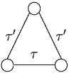
The nodes of the diagram stand for the simple roots. A direct link between two nodes indicates that the two roots are not orthogonal in the Euclidean plane spanned by them. Two roots are orthogonal if there is no direct link between the corresponding nodes. The label attached to a link is determined by the off-diagonal matrix element of the Cartan matrix: no label is shown if such element is ; if it is , the link is labeled by ; if the matrix element is , the label is .
The reflection with respect to the plane orthogonal to and passing through the origin is defined by the general formula (3), where now one has to use the roots of rather than those of . Similarly, the affine reflection is defined as the reflection in the plane orthogonal to and passing through the point . Due to the different normalization of the bases and , some modification appears in the corresponding formulas. Thus instead of (4), we now have
Note the instructive particular cases
The product of the reflections is the translation operator .
| (13) | ||||
Explicitly in the -basis, we have
| (14) | ||||||||
The reflections are subject to the group identities (21), namely,
| (15) |
In contrast to and , the translation can be repeated any number of times without producing the same points.
Below, these transformations are used in order to build 2-dimensional quasicrystalline point sets similarly as in the previous case for the root lattice. Straightforwardly repeated applications of the three operations in every possible sequence, without further restrictions, would produce a dense point set covering the whole plane. Note that if the coordinates of the seed point are in , every point of the set has its coordinates in .
3.2. The case of as an affine extension of
The root system of consists of 30 roots; they can be found in [5]. Relative to an orthonormal basis, normalized to length rather than like in the preceeding subsection, they can be modeled as
| (16) |
Geometrically, the root polytope of is formed by 12 equilateral pentagons and 20 equilateral triangles. It has 30 vertices given by the elements in and 60 edges. It is possible and sometimes advantageous to consider the roots of given in (16) as purely imaginary quaternions of special kind, called icosians [26, 6].
A possible choice of simple roots in the orthonormal basis is
The Cartan matrix of and its inverse,
are used to find
The highest root is .
The affine extension of the Cartan matrix, , and the simple roots in the -basis are
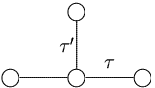
This corresponds to the graph in Fig. 2.
3.3. The case of as an affine extension of
The root system of contains 120 roots, they are found in [5] in terms of simple roots. They can be modeled [6] as the set,
| (18) |
in an orthonormal basis, or equivalently as quaternions [26, 6]. Equipped with quaternionic multiplication, they stand for the elements of the icosahedral group.
As simple roots, one may choose
| (19) | ||||||
The highest root of is then . The -Cartan matrix and its inverse are as follows:
As generalized Cartan matrix and simple roots in the -basis, we obtain
and the corresponding Coxeter diagram is depicted in Fig. 3.

The translation and the four reflections act in 4-space on a point with coordinates in the -basis according to:
| (20) | ||||
Here, as in (8),(14),(17), the reflections are cyclic operations of order two, while the translation can be repeated any number of times. Products of two reflections are rotations around the origin. Their order is determined by the matrix elements of the corresponding Cartan matrix
| (21) |
4. Construction of -induced quasicrystals
In this section, we illustrate an application of the transformations (14), (17) and (20) in order to generate point sets in Euclidean spaces of dimensions 2, 3, and 4, respectively, which resemble fragments of quasicrystals. More precisely, the number of allowed translations plays a similar role as the acceptance window of a cut-and-project quasicrystal and a certain neighbourhood of the seed point contains all the points of such a quasicrystal and only at the periphery the fragment has fewer points. The idea ofthe construction is to use the reflections on a given seed point in every possible way, while using the translation only for a fixed finite number of times.
We start by describing the construction in detail for the case of , after that the other two cases are straightforward.
Transformations (14) acting in 2-space can be represented using matrices. For notational convenience, we use the symbol also for the column matrix :
| (22) |
A straightforward calculation shows that also
In order to change to Cartesian coordinates, a further transformation is needed:
| (23) |
Note that the transformations and act as reflections at the mirrors perpendicular to the simple roots of , which are collinear with the -basis and intersecting at the origin. Their relative angle is and defines a translation along their bisector.
The iterate action of the transformations , and in arbitrary order starting from the origin leads to a point set which fills the plane densely after an infinite number of iterations. If the iteration is stopped after a finite number of steps, a discrete point set is obtained. The application of and transforms a point within the same -orbit. They are equidistant from the origin. Points translated by are on different -orbits. All the points generated by the three operators from one seed point are within one -orbit.
Definition 4.1.
A point is said to be dominant precisely if its coordinates in the -basis are non-negative.
It is convenient to characterize an orbit of by its unique point (dominant point) which is the only one in its orbit with non-negative coordinates in the -basis. It is easily recognizable by this property. Since dominant points encode the information about the whole -orbit, they are a useful tool for the construction and analysis of the point sets.
The size of an -orbit is readily found from its dominant representative by the following rule:
Here, denotes the transposition of the row matrix .
For example, applying and to , , according to (22), one gets the following five points of the orbit, which correspond to the vertices of an equilateral pentagon centered at the origin:
| (24) |
Similarly starting from the point , , one gets another -point orbit consisting of the negatives of (24). Any further application of and would bring no new point.
The square length of the vectors given in the -basis is calculated using the inverse of the Cartan matrix (11):
Definition 4.2.
Let denote the origin of coordinates, and let denote the set of all words formed by the letters , and in which appears precisely times. The set of points
| (25) |
is called an -induced quasicrystal fragment; is the cut-off-parameter.
Due to the identities (21), the point set is finite and -symmetric with respect to the origin. More precisely, the fact that we allow an arbitrary number of actions of and after each translation enforces the finite patches to have circular boundaries. We make this assumption here in view of applications, because this is the situation one encounters e.g. for carbon onions in the study of fullerenes, or, this is what we expect for the growth process of a quasicrystal fragment which is not exposed to any particular obstacles. We remark that it is possible to change (25) by requiring that after the last translation, no further actions of or take place. In this case, -symmetry with respect to the origin would no longer be present in the model.
Note that due to -symmetry, each can be decomposed into concentric shells containing all the points at the same distance from the origin. In general each shell is a union of several decagons and pentagons, except for the origin which alone is a one-point shell. The outer most shell of is the equilateral decagon with dominant point , where translation operators are applied to the origin.
Clearly is just one point, the dominant point . The set contains the origin and the vertices of the decagon of roots. Among the latter the highest root is the dominant one. Thus contains eleven points. It is the union of and the orbit of the roots of :
| (26) |
The equality of the words here and the absence of words involving are consequences of the defining identities (21) of the group . Further applications of and yield no new points.
The set is obtained by shifting by , i.e. by the highest root , and by applying to the result all possible ’s. It contains 61 distinct points.
It decomposes into the sum of four orbits of 10 points with the dominant points
| (27) |
four orbits of 5 points with dominant points
| (28) |
and the origin.
Compare with Fig. 4, where is depicted.
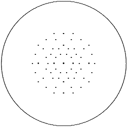
In our construction plays a similar role as the acceptance windows for cut-and-project quasicrystals, because it ensures that instead of a dense set, a discrete point set is obtained. It is therefore interesting to identify as a subset of points of a cut-and-project set as far as possible.
Recall that a cut-and-project point set is completely determined by its acceptance window. There is a 1–1 map between the points of the window and of the cut-and-project set. A finite fragment of an (infinite) cut-and-project point set allows to determine its acceptance window only within certain bounds [23]. The larger is the fragment, the tighter are the bounds on the window. All the points of are found inside of the decagon formed by the outermost shell whose points are at the distance from the origin, where corresponds to the length of any root.
Note that is invariant under 10-fold rotational symmetry by construction. It would also be possible to define an aperiodic point set based on the operations , and which does not have this property. One may e.g. take instead of all sequences which end after the operation in order to break this symmetry.
5. Generalization to and
An extension of the previous construction to 3 and 4 dimensions is straightforward. In analogy to the previous section, we obtain the following operators and from (17) and (20).
- (1)
For and a vector with coordinates in the -basis we have:
(29) (30) - (2)
For and a vector with coordinates in the -basis we have:
(31) (32) (33)
In both cases, the orbit sizes can be found in [5].
Definition 5.1.
Let denote the set of all sequences formed by the operators and in which appears precisely times; O denotes the origin of coordinates. Then
| (34) |
is called -induced quasicrystal fragment for ; is the cut-off-parameter.
Note that describes a -dimensional point set.
6. Investigation of -induced quasicrystals
In this section we analyze the point sets which have been defined in Def. 4.2. Recall that the set was obtained from the origin via an application of three operations, the translation and the reflections and subject to the condition that the operation occurs precisely times, whereas any number of reflections is permitted. As pointed out before, the point set is characterized by its dominant points.
6.1. The dominant points with :
We start by an investigation of the dominant points with . Note that they are given by multiples of the highest root and are thus located on the line . We introduce the notation for the finite point set given as the intersection of the 2-dimensional point set with the line :
| (35) |
The first step in our analysis of will be a description and analysis of .
For the remainder of this paper, we model the root system of in (10) in the complex plane by where
| (36) |
that is number the roots of unity anticlockwise starting from . We remark that due to the 10-fold rotational symmetry of , the set in (35) coincides – when viewed as a 1 dimensional point set – with the sets
| (37) |
Thus, the results obtained for any with translate immediately into each other.
6.1.1. Description of :
We start by expressing the points in in a more convenient way. For this, recall that by definition
| (38) |
where denotes the origin and for denotes a product of basic reflections and , i.e. an element of . We remark that this way of expressing points in is not unique, and different choices of from may lead to the same points in .
Then one has based on (36):
Proposition 6.1.
| (39) |
Thus, consists of all linear combinations of up to (not necessarily different) roots from .
Proof.
It is a consequence of the fact that in (38) is a translation by a root from and the fact that , , act as linear transformations on . In particular, for any tuple , there exists a tuple with such that
| (40) |
Thus, there exists a tuple with
| (41) |
and the claim follows from (38) since the in (41) may represent any element of . ∎
Hence, according to (35) and Proposition 6.1, we know that is the point set which corresponds to all points which are obtained by a linear combinations of up to elements from and lie on the line :
| (42) |
The point set is thus characterized by the values in (42). It is our aim to determine the values of in the following, and we aim at finding for given all with
| (43) |
where , and .
We remark that in order to facilitate notation, we will consider in the following the set where is one of the simple roots. As mentioned before, it coincides with when viewed as a one-dimensional point set without orientation in , and the advantage of considering this set lies in the fact that all points are multiplied by instead of .
We start by setting up some terminology:
Definition 6.2.
Let . Then we call the parameter in the (growth-) level of and the points in are called points of level .
Observe that the th level consists of all points which are linear combinations of exactly elements from , i.e.
| (44) |
Then we have
Proposition 6.3.
consists of the points .
Proof.
corresponds to , corresponds to , to , to and to . No other combinations are possible. ∎
Definition 6.4.
A combination is called reducible if it can be decomposed as where , and . Otherwise, it is called nontrivial.
Lemma 6.5.
If a nontrivial combination exists on level , then it is a combination of elements from .
Proof.
Any combination which contains any of the pairs , , , , or, at least one of the roots and , is necessarily reducible by Proposition 6.3 to configurations on level 2 and 1. Furthermore, any combination containing simultaneously and is reducible to a combination on level . Thus only combinations from or are potentially leading to nontrivial combinations on level . Since both sets give rise to the same one-dimensional point set, the claim is proven. ∎
Theorem 6.6.
There is no nontrivial combination on level .
Proof.
According to Lemma 6.5 any nontrivial combination on level would be of the form
| (45) |
Denote the lattice spanned by and as and the one spanned by and as (see Fig. 5, 6), i.e. define
| (46) |
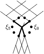
Here and , as well as and denote the diagonals of the parallelograms which constitute the lattices and , respectively.
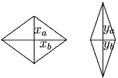
They serve as an orthogonal basis for the lattices and and are of the following lengths:
| (47) |
A necessary condition for a nontrivial combination to exist is thus that there exist and as in (46) such that
| (48) |
However, this implies and , which proves the claim. ∎
Based on Theorem 6.6 we have
Corollary 6.7.
| (49) |
Proof.
Follows via from a decomposition of each level into the contributions from level 2 and 1. ∎
Note, that correspondingly
| (50) |
describes the dominant points with .
6.1.2. Comparison with cut-and-project quasicrystals:
The advantage of expressing as in (49) is the fact that it facilitates comparison with the cut-and-project scheme. For this purpose, we briefly recall the definition of a one-dimensional cut-and-project quasicrystal associated with the irrationality ( see [22] and references within):
Consider the algebraic number field and its nontrivial automorphism denoted by ′ and defined by with . In particular, ′ transforms into . Furthermore, denote the ring of integers of by . Then we have:
Definition 6.8.
Let be a bounded interval. The point set
| (51) |
is called cut-and-project quasicrystal, and the interval is called the acceptance window of .
Based on this, we obtain:
Proposition 6.9.
| (52) |
Proof.
Clearly, implies . Furthermore, and , thus . ∎
Note that the opposite inclusion does not hold, so that the two sets are not equal:
Lemma 6.10.
The inclusion in Proposition 6.9 is a true inclusion. Deficiencies occur for .
Proof.
Let and suppose w.l.o.g. that . Then is bounded by
| (53) |
Fix the -component. Then a sufficient condition for the existence of an fulfilling (53) is
| (54) |
which implies
| (55) |
On the other hand, for we have
| (56) |
where
| (57) |
Since for , deficiencies occur. ∎
We remark that for , the point sets coincide and that deficiencies indeed occur only for .
Example:
In the case , and , which is consistent with but .
Corollary 6.11.
does not correspond to a cut-and-project quasicrystal with connected acceptance window for .
Note that as a consequence of Proposition 6.9 we obtain a lower bound for the minimal distance between adjacent points in :
Lemma 6.12.
The minimal distance in is greater or equal to the one in .
We remark that the latter has been determined in [21] and varies in dependence on the size of the acceptance window.
Finally, let us make a remark about the repetitivity and scaling properties of patterns in . As follows from (49) we have:
- •
For any pattern with and we have . Thus, multiple pattern repetitions occur with growing .
- •
For any there exists , , such that , as follows from
(58)
6.2. Implications for dominant points with
In this subsection, we use the information on the dominant points with derived previously in order to infer information also about the case.
We start by showing:
Theorem 6.13.
For each there exist and such that .
Note that the above statement is trivial if we replace by and needs to be proven only for the case that the cut-off parameter of the (-)subspaces coincides with the cut-off of the two-dimensional (-)setting.
Proof.
Let . Then , where with and as in (36). Expressing for in terms of and leads to
| (59) |
On the other hand,
| (60) |
where .
We thus have to show that for all with there exist , and with such that the following equalities hold:
| (61) |
With the definitions
| (62) |
this is equivalent to showing that for all with there exist and such that and .
For this, we investigate minima and maxima of these functions in dependence on the parameter ranges. In particular, we have
| (63) |
The choices of parameters leading to different qualitative behaviour of and are discussed separately. For instance, for the minimum of the function is at and we have
| (64) |
The other cases can be treated analogously, which proves the claim. ∎
Let denote the cone enclosed by the halflines and . Then this theorem shows that any point in can be expressed as a linear combination of points from and when viewed as vectors in . Since the points in describe the whole point set due to 10-fold rotational symmetry, it follows that any dominant point in can be expressed as a linear combination of points from and for suitably chosen . In particular, dominant points with are given by linear combinations from and , and dominant points with are given by linear combinations from and .
We remark that some of the properties proven here are rooted in the special structure of the ring of cyclotomic integers, which based on (36) is given by
| (65) |
and of which is by construction a subset.
We can again embed our point set into a cut-and-project quasicrystal. For this, we indicate briefly how the setting of cut-and-project quasicrystals as introduced in Definition 6.8 can be generalized to two dimensional point sets with symmetry (see [28] and references within for more details):
Definition 6.14.
Let denote a -lattice with respect to some basis in . Then we call the map with the property for all , and a -map.
Definition 6.15.
Let be a -lattice in and a bounded region in , called acceptance window. Then
| (66) |
defines a cut-and-project quasicrystal in dimensions.
In order to construct a cut-and-project quasicrystal with symmetry along these lines, one takes as -lattice in in Def. 6.15, and as ∗-map, one uses based on (36)
| (67) |
which fulfills the requirements of a -map (cf. Def. 6.14) and leaves invariant:
| (68) |
With this, a cut-and-project quasicrystal as in (69) can be parameterized as
| (69) |
where may be any bounded region in .
Note in particular that and (compare with (36)).
Based on this, we find the following in our context:
Lemma 6.16.
Let denote the convex hull of the regular decagon inscribed into a circle of radius around the origin and let denote the corresponding cut-and-project quasicrystal. Then
| (70) |
Proof.
implies with , and . Thus, . Since leaves invariant, and the claim follows. ∎
As before, there is no equality in Lemma 6.16 and for deficiencies occur. Also, minimal distances in are bounded from below by the ones in .
7. Conclusion
We have suggested a new way to construct mathematical models for fragments of aperiodic point sets with 10-fold symmetry. Like cut-and-project quasicrystals, they require some cut-off condition which prevents the sets from becoming dense. The special feature of these models is that they are by construction finite structures – not idealized infinite ones – which grow from a seed point as we demonstrate in Appendix B. We have shown that they are not fragments of sets obtainable via the cut-and-project scheme for convex windows. The restriction to convex windows is a plausible assumption when dealing with growth processes which are not hindered by obstacles. In the presence of obstacles, points would be generated around them and the corresponding acceptance windows would not necessarily be convex and connected. The deviation of our point sets from the cut-and-project situation with convex windows is given in terms of a set of “deficiencies”, which appear close to the boundary of the set. The occurrence of deficiencies is a novel aspect and a special feature of our models, and it has to be discussed in how far it may help to model growth deficiencies which occur in real life quasicrystals.
Finally, we remark that though our initial motivation for this study comes from the field of quasicrystals, we expect that the mathematical structures provided by the affine extension of noncrystallographic Coxeter groups will open also other fields of applications. We plan to investigate in a next step the application of our results to the study of fullerenes, in particular the description of onion like structures and nanotubes.
Acknowledgements
J. P. acknowledges financial support by the Natural Sciences and Engineering Research Council of Canada and FCAR of Quebec and R. T. by a Marie Curie fellowship. She is grateful for the hospitality extended to her at the Centre de Recherches Mathématiques, Université de Montréal, where this work has been started.
References
- [1] Antoine J-P, Jacques L and Twarock R 1999 Investigation of a quasiperiodic tiling with fivefold symmetry via wavelet analysis Phys. Lett. A 261 265–274
- [2] Brodsky M H, DiVincenzo D P and Mosseri R 1985 A structural basis for electronic coherence in amorphous Si and Ge Proc of 17th Int. Conf. on the Physics of Semiconductors 803–806
- [3] Brodsky M H, DiVincenzo D P, Sadoc J F and Brodsky M H 1985 Polytope model and the electronic and structural properties of amorphous semiconductors Phys. Rev. B 32 3974–4000
- [4] Bul’enkov N A 1991 Possible role of hydration as the leading integration factor in the organization of biosystems at different levels of their hierarchy Biophysics 36 181–244
- [5] Champagne B, Kjiri M, Patera J and Sharp R 1995 Description of reflection generated polytopes using decorated coxeter diagrams Can. J. Phys. 73 566–584
- [6] Chen L, Moody R V and Patera J 1998 Noncrystallographic root systems Quasicrystals and Discrete Geometry, eds J Patera (Amer. Math. Soc.) vol. 10 of Fields Institute Monograph Series pp 135–178 pp 135–178
- [7] Coxeter H S M 1973 Regular Polytopes (New York: Dover publications)
- [8] DiVincenzo D P 1988 Nonlinear optics as a probe of chiral ordering in amorphous semiconductors Phys. Rev. B 37 1245–1261
- [9] DiVincenzo D P and Brodsky M H 1985 Polytope-like order in random network model of amorphous semiconductors J. Non-Crystall. Solids 77 & 78 241–244
- [10] DiVincenzo D P, Mosseri R, Brodsky M H and Sadoc J F 1984 Long range structural and electronic coherence in amorphous semiconductors Phys. Rev. B 29 5934–5936
- [11] Duneau M, Katz A 1985 Quasiperiodic patterns Phys. Rev. Lett. 54 2688–2691
- [12] Elser V and Sloane N J A 1987 A highly symmetric four-dimensional quasicryslal J.Phys. A: Math. Gen. 20 6161–6167
- [13] Fradkin M A 1987 Phonon spectrum of metallic glasses in an icosahedral model Soviet Phys. – JTEP 66 822–828
- [14] Gross D, Harvey J A, Martinec E and Rhom R 1985 Heterotic strings Phys. Rev. Lett. 54 502–505
- [15] Humphreys J E 1992 Reflection Groups and Coxeter groups Cambridge studies in advanced mathematics 29 (Cambridge Univ. Press)
- [16] Janot C 1994 Quasicrystals: A Primer, 2nd. Edition (Oxford: Oxford Univ. Press)
- [17] Kac V 1985 Infinite Dimensional Lie Algebras (Cambridge: Cambridge University Press)
- [18] Kass S, Moody R V, Patera J and Slansky R 1990 Affine Lie Algebras, Weight Multiplicities and Branching Rules (Los Angeles: Univ. of Calif. Press)
- [19] Kroto H W 1992 Carbon onions introduce new flavour to fullerene studies Nature 359 670
- [20] Masáková Z, Patera J and Pelantová E 1998 Inflation centers of the cut and project quasicrystals J. Phys. A: Math. Gen. 31 1443–1453
- [21] Masáková Z, Patera J and Pelantová E 1998 Minimal distances in quasicrystals J. Phys. A: Math. Gen. 31 1539–1552
- [22] Masáková Z, Patera J and Pelantová E 1998 Quadratic irrationalities and geometric properties of one-dimensional quasicrystals CRM-2565
- [23] Masáková Z, Patera J and Pelantová E 1998 Seldimilar Delone sets and qusicrystals J. Phys. A: Math. Gen. 31 4927–4946
- [24] Moody R V 2000 Model sets: A survey From Quasicrystals to More Complex Systems, eds F Axel, Dénoyer F, Gazeau J.-P. (Springer) 145–166
- [25] Moody R V 1997 Meyer sets and their duals Mathematics of Long Range Aperiodic Order, eds R V Moody (Kluwer) 403–441
- [26] Moody R V and Patera J 1993 Quasicrystals and icosians J. Phys. A: Math. Gen. 26 2829–2853
- [27] Patera C S L J and Sharp R T 1996 Generating functions for the Coxeter group J.Phys. A: Math. Gen. 29 2829–2853
- [28] Patera J 1997 Noncrystallographic root systems and quasicrystals Mathematics of Long Range Aperiodic Order, eds R V Moody (Kluwer)
- [29] Scherbak O P 1988 Wavefronts and reflection groups Russian Math. Surveys 43(3) 149–194
- [30] Shechtman D, Blech I, Gratias D and Cahn J 1984 Metallic phase with long-range order and no translational symmetry Phys. Rev. Lett. 53
- [31] Zuber J B 1996 Graphs and reflection groups Commun. Math. Phys. 179 265–294
- [32] Zuber J B 1998 Generalized dynkin diagrams and root systems and their folding Prog. Math. 160 453–491
Appendix A
In this appendix, we indicate the generalized Cartan matrices obtained after relaxation of the condition (compare with Section 3). In particular, let , , and be the entries of the matrices
| (71) |
Then the entries in the following tables define generalized Cartan matrices for (first matrix in (71) and Table 1), (second matrix in (71) and Table 2) and (third matrix in (71) and Table 3), respectively.
Table 1: the case of
| -2 | 0 | 0 | 1 |
| -1 | 1 | -1 | 1 |
| -1 | 1 | 0 | -1 |
| 0 | -1 | -1 | 1 |
| 0 | -1 | 2 | 0 |
| 0 | 1 | -2 | 0 |
| 0 | 1 | 1 | -1 |
| 1 | -1 | 0 | 1 |
| 1 | -1 | 1 | -1 |
| 2 | 0 | 0 | -1 |
Table 2: the case of
| -2 | 0 | 1 | 0 | 0 | 0 |
| -1 | -2 | 0 | 2 | -2 | 1 |
| -1 | 1 | 0 | -1 | 1 | 0 |
| -1 | 1 | 0 | 0 | -1 | 0 |
| -1 | 1 | 1 | -1 | 1 | 0 |
| -1 | 1 | 1 | 0 | -1 | 0 |
| 0 | -3 | -1 | 2 | -1 | 1 |
| 0 | -1 | -1 | 1 | -1 | 1 |
| 0 | 0 | -1 | 1 | 0 | 0 |
| 0 | 0 | 0 | -1 | 2 | 0 |
| 0 | 0 | 0 | 1 | -2 | 0 |
| 0 | 0 | 1 | -1 | 0 | 0 |
| 0 | 1 | 1 | -1 | 1 | -1 |
| 0 | 3 | 1 | -2 | 1 | -1 |
| 1 | -1 | -1 | 0 | 1 | 0 |
| 1 | -1 | -1 | 1 | -1 | 0 |
| 1 | -1 | 0 | 0 | 1 | 0 |
| 1 | -1 | 0 | 1 | -1 | 0 |
| 1 | 2 | 0 | -2 | 2 | -1 |
| 2 | 0 | -1 | 0 | 0 | 0 |
Table 3: the case of
| -2 | 0 | 1 | 0 | 0 | 0 | 0 | 0 |
| -1 | 0 | -1 | 0 | 1 | 0 | 0 | 0 |
| -1 | 0 | 0 | 0 | -1 | 0 | 0 | 1 |
| -1 | 0 | 0 | 0 | 0 | 0 | -1 | 1 |
| -1 | 0 | 0 | 0 | 0 | 1 | 0 | -1 |
| -1 | 0 | 0 | 0 | 1 | -1 | 1 | 0 |
| -1 | 0 | 0 | 0 | 1 | 0 | -1 | 0 |
| -1 | 0 | 0 | 0 | 1 | 0 | 1 | -1 |
| -1 | 0 | 0 | 1 | 0 | -1 | 1 | 0 |
| -1 | 0 | 0 | 1 | 0 | 0 | -1 | 0 |
| -1 | 0 | 0 | 1 | 1 | -1 | 0 | 0 |
| -1 | 0 | 1 | -1 | -1 | 1 | 0 | 0 |
| -1 | 0 | 1 | -1 | 0 | 0 | 1 | 0 |
| -1 | 0 | 1 | -1 | 0 | 1 | -1 | 0 |
| -1 | 0 | 1 | 0 | -1 | 0 | -1 | 1 |
| -1 | 0 | 1 | 0 | -1 | 0 | 1 | 0 |
| -1 | 0 | 1 | 0 | -1 | 1 | -1 | 0 |
| -1 | 0 | 1 | 0 | 0 | -1 | 0 | 1 |
| -1 | 0 | 1 | 0 | 0 | 0 | 1 | -1 |
| -1 | 0 | 1 | 0 | 1 | 0 | 0 | -1 |
| -1 | 0 | 2 | 0 | -1 | 0 | 0 | 0 |
| -1 | 1 | 0 | -1 | 0 | 0 | 1 | 0 |
| -1 | 1 | 0 | -1 | 0 | 1 | -1 | 0 |
| -1 | 1 | 0 | -1 | 1 | 0 | 0 | 0 |
| -1 | 1 | 0 | 0 | 0 | -1 | 0 | 1 |
| -1 | 1 | 0 | 0 | 0 | 0 | 0 | 0 |
| -1 | 1 | 0 | 0 | 1 | 0 | 0 | -1 |
| -1 | 1 | 1 | -1 | -1 | 0 | 0 | 1 |
| -1 | 1 | 1 | -1 | 0 | 0 | 0 | 0 |
| -1 | 1 | 1 | -1 | 0 | 1 | 0 | -1 |
| -1 | 1 | 1 | 0 | -1 | 0 | 0 | 0 |
| -1 | 1 | 1 | 0 | 0 | -1 | 1 | 0 |
| -1 | 1 | 1 | 0 | 0 | 0 | -1 | 0 |
| 0 | -1 | -1 | 1 | 0 | 0 | 0 | 0 |
| 0 | -1 | -1 | 1 | 1 | -1 | 1 | 0 |
| 0 | -1 | -1 | 1 | 1 | 0 | -1 | 0 |
| 0 | -1 | 0 | 0 | -1 | 1 | 0 | 0 |
| 0 | -1 | 0 | 0 | 0 | 0 | -1 | 1 |
| 0 | -1 | 0 | 0 | 1 | 0 | 1 | -1 |
| 0 | -1 | 0 | 1 | -1 | 0 | -1 | 1 |
| 0 | -1 | 0 | 1 | 0 | 0 | 1 | -1 |
| 0 | -1 | 0 | 1 | 1 | -1 | 0 | 0 |
| 0 | -1 | 1 | 0 | -1 | 0 | 1 | 0 |
| 0 | -1 | 1 | 0 | -1 | 1 | -1 | 0 |
| 0 | -1 | 1 | 0 | 0 | 0 | 0 | 0 |
| 0 | 0 | -1 | 0 | 0 | 0 | -1 | 1 |
| 0 | 0 | -1 | 0 | 0 | 0 | 1 | 0 |
| 0 | 0 | -1 | 0 | 0 | 1 | -1 | 0 |
| 0 | 0 | -1 | 0 | 1 | -1 | 0 | 1 |
| 0 | 0 | -1 | 0 | 1 | 0 | 1 | -1 |
| 0 | 0 | -1 | 0 | 2 | 0 | 0 | -1 |
| 0 | 0 | -1 | 1 | 0 | -1 | 0 | 1 |
| 0 | 0 | -1 | 1 | 1 | -1 | 0 | 0 |
| 0 | 0 | -1 | 1 | 1 | 0 | 0 | -1 |
| 0 | 0 | 0 | -1 | -1 | 1 | -1 | 1 |
| 0 | 0 | 0 | -1 | 0 | 1 | 1 | -1 |
| 0 | 0 | 0 | -1 | 1 | 0 | 0 | 0 |
| 0 | 0 | 0 | 0 | -1 | 0 | 1 | 0 |
| 0 | 0 | 0 | 0 | -1 | 1 | -1 | 0 |
| 0 | 0 | 0 | 0 | 0 | -1 | 2 | 0 |
| 0 | 0 | 0 | 0 | 0 | 1 | -2 | 0 |
| 0 | 0 | 0 | 0 | 1 | -1 | 1 | 0 |
| 0 | 0 | 0 | 0 | 1 | 0 | -1 | 0 |
| 0 | 0 | 0 | 1 | -1 | 0 | 0 | 0 |
| 0 | 0 | 0 | 1 | 0 | -1 | -1 | 1 |
| 0 | 0 | 0 | 1 | 1 | -1 | 1 | -1 |
| 0 | 0 | 1 | -1 | -1 | 0 | 0 | 1 |
| 0 | 0 | 1 | -1 | -1 | 1 | 0 | 0 |
| 0 | 0 | 1 | -1 | 0 | 1 | 0 | -1 |
| 0 | 0 | 1 | 0 | -2 | 0 | 0 | 1 |
| 0 | 0 | 1 | 0 | -1 | 0 | -1 | 1 |
| 0 | 0 | 1 | 0 | -1 | 1 | 0 | -1 |
| 0 | 0 | 1 | 0 | 0 | -1 | 1 | 0 |
| 0 | 0 | 1 | 0 | 0 | 0 | -1 | 0 |
| 0 | 0 | 1 | 0 | 0 | 0 | 1 | -1 |
| 0 | 1 | -1 | 0 | 0 | 0 | 0 | 0 |
| 0 | 1 | -1 | 0 | 1 | -1 | 1 | 0 |
| 0 | 1 | -1 | 0 | 1 | 0 | -1 | 0 |
| 0 | 1 | 0 | -1 | -1 | 1 | 0 | 0 |
| 0 | 1 | 0 | -1 | 0 | 0 | -1 | 1 |
| 0 | 1 | 0 | -1 | 1 | 0 | 1 | -1 |
| 0 | 1 | 0 | 0 | -1 | 0 | -1 | 1 |
| 0 | 1 | 0 | 0 | 0 | 0 | 1 | -1 |
| 0 | 1 | 0 | 0 | 1 | -1 | 0 | 0 |
| 0 | 1 | 1 | -1 | -1 | 0 | 1 | 0 |
| 0 | 1 | 1 | -1 | -1 | 1 | -1 | 0 |
| 0 | 1 | 1 | -1 | 0 | 0 | 0 | 0 |
| 1 | -1 | -1 | 0 | 0 | 0 | 1 | 0 |
| 1 | -1 | -1 | 0 | 0 | 1 | -1 | 0 |
| 1 | -1 | -1 | 0 | 1 | 0 | 0 | 0 |
| 1 | -1 | -1 | 1 | 0 | -1 | 0 | 1 |
| 1 | -1 | -1 | 1 | 0 | 0 | 0 | 0 |
| 1 | -1 | -1 | 1 | 1 | 0 | 0 | -1 |
| 1 | -1 | 0 | 0 | -1 | 0 | 0 | 1 |
| 1 | -1 | 0 | 0 | 0 | 0 | 0 | 0 |
| 1 | -1 | 0 | 0 | 0 | 1 | 0 | -1 |
| 1 | -1 | 0 | 1 | -1 | 0 | 0 | 0 |
| 1 | -1 | 0 | 1 | 0 | -1 | 1 | 0 |
| 1 | -1 | 0 | 1 | 0 | 0 | -1 | 0 |
| 1 | 0 | -2 | 0 | 1 | 0 | 0 | 0 |
| 1 | 0 | -1 | 0 | -1 | 0 | 0 | 1 |
| 1 | 0 | -1 | 0 | 0 | 0 | -1 | 1 |
| 1 | 0 | -1 | 0 | 0 | 1 | 0 | -1 |
| 1 | 0 | -1 | 0 | 1 | -1 | 1 | 0 |
| 1 | 0 | -1 | 0 | 1 | 0 | -1 | 0 |
| 1 | 0 | -1 | 0 | 1 | 0 | 1 | -1 |
| 1 | 0 | -1 | 1 | 0 | -1 | 1 | 0 |
| 1 | 0 | -1 | 1 | 0 | 0 | -1 | 0 |
| 1 | 0 | -1 | 1 | 1 | -1 | 0 | 0 |
| 1 | 0 | 0 | -1 | -1 | 1 | 0 | 0 |
| 1 | 0 | 0 | -1 | 0 | 0 | 1 | 0 |
| 1 | 0 | 0 | -1 | 0 | 1 | -1 | 0 |
| 1 | 0 | 0 | 0 | -1 | 0 | -1 | 1 |
| 1 | 0 | 0 | 0 | -1 | 0 | 1 | 0 |
| 1 | 0 | 0 | 0 | -1 | 1 | -1 | 0 |
| 1 | 0 | 0 | 0 | 0 | -1 | 0 | 1 |
| 1 | 0 | 0 | 0 | 0 | 0 | 1 | -1 |
| 1 | 0 | 0 | 0 | 1 | 0 | 0 | -1 |
| 1 | 0 | 1 | 0 | -1 | 0 | 0 | 0 |
| 2 | 0 | -1 | 0 | 0 | 0 | 0 | 0 |
Appendix B
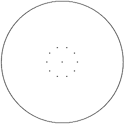
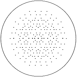
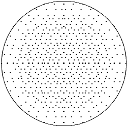
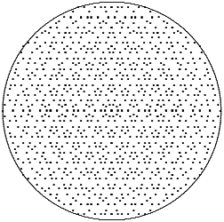
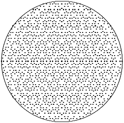
In this appendix we demonstrate the growth of in dependence on for . Note that we display the point sets in a circle of a radius corresponding to four times the root length. Thus, the complete point set is visible only until iteration step and is truncated afterwards. Note that since the point set is displayed in Fig. 4 we omit it in this list.