Moduli Spaces of Abelian Differentials:
The Principal Boundary,
Counting Problems,
and the Siegel–Veech ConstantsThanks: Research of the first author is partially supported by
NSF grant DMS-9704845, the Sloan
Foundation and the Packard FoundationThanks: Research of the second author is partially supported by
NSF grant 9803497
Abstract.
A holomorphic 1-form on a compact Riemann surface naturally defines a flat metric on with cone-type singularities. We present the following surprising phenomenon: having found a geodesic segment (saddle connection) joining a pair of conical points one can find with a nonzero probability another saddle connection on having the same direction and the same length as the initial one. A similar phenomenon is valid for the families of parallel closed geodesics.
We give a complete description of all possible configurations of parallel saddle connections (and of families of parallel closed geodesics) which might be found on a generic flat surface . We count the number of saddle connections of length less than on a generic flat surface ; we also count the number of admissible configurations of pairs (triples,…) of saddle connections; we count the analogous numbers of configurations of families of closed geodesics. By the previous result of [EMa] these numbers have quadratic asymptotics . Here we explicitly compute the constant for a configuration of every type. The constant is found from a Siegel—Veech formula.
To perform this computation we elaborate the detailed description of the principal part of the boundary of the moduli space of holomorphic 1-forms and we find the numerical value of the normalized volume of the tubular neighborhood of the boundary. We use this for evaluation of integrals over the moduli space.
Introduction
1. Flat Surfaces and Geodesics on Flat Surfaces
In this paper we shall consider flat metrics with isolated conical singularities on a closed orientable surface of genus . An important class of such flat metrics corresponds to the translation surfaces: those surfaces for which the flat metric on the surface has trivial linear holonomy. These surfaces have been studied by several authors in various guises; in the context of Abelian differentials (and more generally quadratic differentials) on compact Riemann surface in [S], in the context of rational billiards in [KaZe], [KMS], [Ve3], and [GJ]. Moduli spaces of these structures have been studied in [Ve4 ], [MS], [Ko], [KonZo], and [EMa]. A survey is given in [MT].
Triviality of holonomy means, in particular, that the parallel transport of a vector along a small loop going around a conical point brings a vector back to itself. This implies that all cone angles of such surface are integer multiples of .
Choose a direction in the tangent space to some base point of the flat surface and transport this direction using the parallel transport to all nonsingular points of the surface. Since the monodromy is trivial this parallel transport does not depend on the path. Thus, any direction is globally defined on the flat surface punctured at the singularities. Throughout this paper by a flat surface we mean a flat surface having trivial holonomy representation in . Following a tradition we often call the conical points the saddles.


A flat torus gives an example of a flat surface without any saddles. One can glue a flat torus from a parallelogram by identifying opposite sides. A generalization can be found by considering a polygon in the plane having the property that its sides are distributed into pairs that are parallel and of equal length. Identifying the pairs by translations one gets a closed oriented flat surface. For example, identifying the opposite sides of a regular octagon one gets a surface of genus , see Figure 1. All vertices of the octagon are identified to a single saddle which has an angle of . Deforming the regular octagon in such way that the sides are organized into pairs of parallel sides of equal length we get a family of flat surfaces of genus each having a single conical singularity with the cone angle .
We may assume that we have cartesian coordinates in the polygons. In these coordinates away from the saddles, geodesics on the surface are straight lines. The behavior of geodesics on flat surfaces is in many aspects similar to the behavior of geodesics on a flat torus. In particular, a geodesic cannot change the direction, and thus cannot have self intersections. A generic geodesic is dense in the surface analogously to an irrational winding line which is dense on the torus.
However, a flat surface different from the torus must have saddles and some geodesics that hit the saddles. Some geodesics hit the saddles going both in forward and in backward directions. Such a geodesic segment joining a pair of saddles and having no saddles in its interior is called a saddle connection.
Note that the shortest representative in a homotopy class of curves joining two saddles exists. Typically, even for the class of a simple closed curve, one gets a broken line containing many geodesic segments. The segments of these broken lines pass through the saddles changing directions there. We want to stress that throughout this paper we consider only those saddle connections which contain a single geodesic segment and thus no saddles in its interior. However, we consider the situation when the endpoints of a saddle connection coincide. We call such saddle connections the closed saddle connections.
A geodesic leaving a regular point may return back to without meeting any singularities. Since it cannot change its direction, we necessarily get a closed regular geodesic in this case. Note that as in the case of the torus, any geodesic leaving a nearby point in a parallel direction will be also closed and will have the same length as the initial one. Thus closed regular geodesics appear in families of parallel geodesics of the same length. However, unlike the case of the torus, such parallel closed geodesics do not typically fill all the surface, but only a cylindrical subset. Each boundary component of such a cylinder is comprised of saddle connections. For example, choosing the vertical direction on the flat surface obtained from a regular octagon (see Figure 1) we get two families of regular closed geodesics, and each of the two families fills a cylinder. Generically, each boundary component of a cylinder filled with closed geodesics is a single closed saddle connection.
The converse, however, is false. A closed saddle connection does not necessarily bound a cylinder of regular closed geodesics. In fact, it bounds such a cylinder if and only if the angle at the saddle between the outgoing and incoming segments is exactly . In this paper we will be interested in both counting closed saddle connections and counting cylinders filled with regular closed geodesics.
Now fix a flat surface . Let be the universal cover of , where is the collection of saddles. There is an isometric map of to called the developing map which maps a lift of an oriented curve on to a curve in . We denote by the difference of the endpoints of the image. The vector is called the holonomy vector of .
Remark 1.1.
By definition a flat surface has trivial holonomy representation in the linear group
However, the holonomy representation in the affine group is nontrivial: its image belongs to the group of translations. From now on we reserve the notion of holonomy for this second representation. It matches the notion of holonomy defined by an arbitrary (not necessarily closed) oriented curve suggested in the paragraph above.
Now fix a pair of saddles on a flat surface , and some length . Consider all those saddle connections joining the fixed saddles whose length is shorter than . We are interested in the asymptotics of the number of saddle connections when the bound tends to infinity. In the model case of the torus of unit area it is sufficient to pass to the universal covering plane to see that the number of geodesic segments of length at most joining a generic pair of distinct points on the torus grows quadratically as the number of lattice points in a disc of radius , so we get asymptotics . Note that the number of (homotopy classes) of closed geodesics of length at most has different asymptotics. Since we want to count only primitive geodesics (those which do not repeat themselves) now we have to count only coprime lattice points in a disc of radius , considered up to a symmetry of the torus (issues of symmetry will be considered in details later). Therefore we get the asymptotics .
It is proved in [EMa] that the growth rate of the number of saddle connections for a generic flat surface also has quadratic asymptotics , and, moreover, almost all flat surfaces in some natural families of flat surfaces share the same constant in the asymptotics. One of the principal goals of this paper is to compute these constants for all natural families (which are explicitly defined below). We also compute the constants in the quadratic asymptotics for the number of families of closed regular geodesics.
It is relatively easy to show that for a generic flat surface one can never find a pair of saddle connections having the same direction but different lengths, see Proposition 7.4 at the end of Section 7. However, somewhat surprisingly, the configurations of pairs of parallel saddle connections of the same length and same direction can be found on almost every flat surface, and, what may seem even more surprising, their number also has quadratic asymptotics (with another constant ).
One can ask now the similar questions about the triples of saddle connections, or about some more specific configurations of saddle connections, or similar questions concerning closed geodesics. We give a complete description of those configurations which can be found on a generic surface; we show that each of them has quadratic asymptotics (this was essentially already proved in [EMa]), and in every case we compute the corresponding constant in the quadratic asymptotics.
Remark 1.2.
A billiard in a polygon with rational angles gives rise to a flat surface, see for example [KaZe], [KMS], or [MT]. However, rational billiards are not generic in the natural families of flat surfaces, which we consider. Thus, the constants described in this paper do not apply to the billiard problem, with an exception for some particular classes off billiards, see [EZo].
1.1. Flat Surfaces and Abelian Differentials
If we cut a flat surface successively along an appropriate collection of saddle connections we can decompose it into polygons contained in , see, for example, Figure 1. We may then view as a union of polygons glued along parallel sides by means of parallel translations. Note that we have endowed every polygon with a complex coordinate. Since our gluing rules are just translations, the transition functions in these complex coordinates have the form
Thus any flat surface with the conical singularities removed is endowed with a natural complex structure. Moreover, consider a holomorphic 1-form on every polygon. Since we obtain a globally defined holomorphic 1-form on the surface with removed singularities. It is an easy exercise to show that the complex structure and the holomorphic 1-form can be extended to the singularities; the holomorphic 1-form (or, what is the same, the Abelian differential) has a zero at every conical point.
Conversely, given a pair where is a Riemann surface, is a holomorphic Abelian differential on , and a point such that , there exists a local coordinate near such that . Such a local coordinate is unique up to change of coordinates . Thus is a flat metric on ; this metric develops conical singularities at the zeroes of . At a zero of order the total angle is . Such collection of coordinate charts determines a structure of a “translation surface” (which we agree to call just a “flat surface”) on , namely, an atlas of coordinate charts which cover the surface away from the singularities, such that the transition functions are translations
When we consider moduli spaces of flat surfaces we will wish to distinguish between and . This is equivalent to specifying a distinguished direction on the flat surface.
Convention 1.
Depending on the context we shall use one of the synonyms “saddle”, “conical singularity”, “zero of Abelian differential” or just “zero”.
2. Moduli Spaces of Abelian Differentials
2.1. Stratification
Let be a partition of (i.e. a representation of as an unordered sum of positive integers). Let denote the moduli space of pairs where is a closed Riemann surface of genus , and is a holomorphic Abelian differential on such that the orders of its zeroes is given by . Here we distinguish between and . The zeroes on each surface are assumed to be named. We say that two such structures are equivalent if there is an isomorphism from one to the other which takes zeroes to zeroes, preserving the naming. The set of equivalence classes is denoted and is called a stratum. This term is justified by the fact that the space of all Abelian differentials on Riemann surfaces of genus is stratified by the spaces , as varies over the partitions of . In the case of flat tori the space is , the moduli space of lattices. The stratum corresponding to the partition is called the principal stratum: it corresponds to holomorphic differentials with simple zeroes. For example, the surface in Figure 2 belongs to . The stratum might be nonconnected, although the components have been completely classified (see [KonZo]). The classification involves the notion of parity of spin structure and issues of hyperellipticity. These components will be described later in Section 5.2.
2.2. Local Coordinates and Volume Element
The stratum can be topologized and given a natural “Lebesgue” measure as follows. For a flat surface with conical points , choose a basis of cycles for the relative homology . This basis may be chosen in such a way that each element is represented by a saddle connection. Equivalently, the saddle connections cut into a union of polygons. For any near the vectors associated to these saddle connections serve as local coordinates, see, for example, Figure 1. By construction these vectors are the relative periods of the Abelian differential (i.e. the integrals of along the paths joining points and , where is also allowed). So we actually use a domain in the space of relative cohomology as a local coordinate chart. Ignoring the complex structure we get a domain in , where . Note that we have a natural cubic lattice in our coordinates given by the “integer” cohomology
We define a measure or volume element on as Lebesgue measure defined by these coordinates, normalized so that the volume of a unit cube in is . One easily checks that the volume element is well-defined: it is independent of choice of basis.
Let be the hypersurface in of unit area flat surfaces. Choose a symplectic homology basis of closed curves , on the surface . The area of the flat surface defined by the Abelian differential is given by the Riemann bilinear relation,
Thus the unit area surfaces represent a “hyperboloid” in terms of the coordinates chosen above.
Throughout this paper we shall mostly work with the “hyperboloid” . The volume element in the embodying space induces naturally a volume element on the hypersurface in the following way. There is a natural -action on : having we associate to the flat surface the flat surface . In particular, we can represent any as , where , and where belongs to the “hyperboloid”: . Geometrically this means that the metric on is obtained from the metric on by rescaling with coefficient . In particular, vectors associated to saddle connections on are multiplied by to give vectors associated to corresponding saddle connections on . It means also that , since . We define the volume element on the “hyperboloid” by disintegration of the volume element on :
where . Using this volume element we define the total volume of the stratum :
| (1) |
Since the measure on is induced by the volume element, the total volume of the stratum coincides with the total measure.
For a subset we let denote the “cone” based on :
| (2) |
Our definition of the volume element on is consistent with the following normalization:
| (3) |
where , and is the total volume (total measure) of the “cone” measured by means of the volume element on defined above.
Convention 2.
We need to use both volume elements. To distinguish them we keep the notation for the volume element in the whole stratum and notation for the volume (hypersurface) element in the “unit hyperboloid” which is a hypersurface in .
It is a result of [M], [MS] and [Ve2] that these volumes are finite. Their values have been calculated in [EOk], see also [Zo] for the volumes of some low-dimensional strata. They will be needed for the calculations of the asymptotic constants. Tables of the values of the volumes for all connected components of the strata in genera are presented in section 8.4.
3. Principal Boundary of the Moduli Spaces and Method of Evaluation of the Siegel—Veech Constants
3.1. Holonomy and Homology
Note that in terms of the local coordinates defining the flat structure the corresponding Abelian differential has the form . This has an important consequence: for any oriented curve on , the holonomy of (as defined above in terms of the developing map) coincides with the integral of over (here we have identified and ). Since the 1-form is closed, it means, in particular, that if and are homologous, then . In particular, if we have a cylinder filled with regular closed geodesics, then all these geodesics share the same holonomy vector.
When a path joins a pair of distinct points we say that a path is homologous to if it joins the same pair of points and if the closed loop is homologous to zero, that is breaks the surface into two components. The paths which interest us in this paper are saddle connections or closed geodesics on . We can formalize the above observation saying that saddle connections representing homologous elements in (where are the saddles) share the same holonomy vector .
On the other hand the equality for nonhomologous occurs only for non generic surfaces. Consider the following example. Take four unit squares with sides glued as indicated at the left-hand-side picture at Figure 2. The result is a closed surface of genus . The five points indicated by the filled circle symbol are identified, as are the five points indicated by the unfilled circle symbol. Hence has two conical singularities, each of total angle . Each of the hatched squares corresponds to a cylinder filled with horizontal regular closed geodesics of length . Hence, for any closed geodesics in the first cylinder and any closed geodesics in the second cylinder we get .
Note, however, that and are not homologous. This means that the relation above does not survive under a generic deformation of this flat surface, see the right-hand-side picture at Figure 2. On the other hand the pair of saddle connections and are homologous and we see that they keep sharing the same holonomy under any small deformation of the surface. Figure 11 gives an example when such a relation between two distinct families of closed geodesics is stable under any small deformation of the flat surface.


This observation can be formalized as follows.
Proposition 3.1.
Almost any flat surface in any connected component of any stratum does not have a single pair of nonhomologous saddle connections sharing the same holonomy vector.
Proof.
Consider a basis of (relative) cycles in . We know that the corresponding periods of (integrals over these basic cycles) serve as local coordinates in the stratum . Note that for almost all points of the cohomology space these periods are rationally independent: no linear combination of periods equals to zero when the linear combination is taken with rational coefficients. Note also, that if the periods of a closed 1-form are rationally independent, then the same property is obviously true for the form where . Hence, this is true for almost all flat surfaces in the “unit hyperboloid”
A pair of saddle connections represent integer cycles in . Hence, if they are not homologous, for almost all points of the corresponding periods are different: . Since and the Proposition is proved. ∎
3.2. Configurations of Saddle Connections
Consider the set of all saddle connections on a flat surface and consider its image under the holonomy map. (We remind the reader that by definition, a saddle connection is represented by a single geodesic segment joining a pair of conical points, and not by a broken line of geodesic segments.)
Choose, for example, a flat torus as a surface and mark a generic pair of points on this torus. Let . The set is the square lattice of the form .
Similarly to the torus case, the set is a discrete subset of . However, when is different from the torus the map from the set of saddle connections on to is not injective: different saddle connections may have the same holonomy. We define the multiplicity of an element to be the number of distinct saddle connections such that . For example, for the surface presented on the left of Figure 2 the vector has multiplicity four: the saddle connections chosen with appropriate orientation have holonomy .
In this example the saddle connections represented by are not pairwise homologous. As indicated above, the fact that their holonomy coincides is not generic; deforming the surface slightly we see that the corresponding saddle connections have different holonomy; see the right-hand-side picture at Figure 2. The situation is different with the saddle connections and , for they are homologous. The right-hand-side picture at Figure 2 confirms that even after any small deformation of the surface the corresponding saddle connections share the same holonomy vector .
From the measure-theoretical point of view Proposition 3.1 allows us to assume from now on that if two saddle connections have the same holonomy, then and are homologous. In particular, if joins distinct saddles , then joins the same pair of saddles. Since the surfaces as in the left-hand-side picture at Figure 2 form a set of measure zero we will ignore them in our considerations.
Somewhat surprisingly, higher multiplicity is very common even for a generic surface. For example, we will show that if the genus is at least , then counting separately the vectors of multiplicity one in of length at most and the vectors of multiplicity two, we get quadratic growth in for the number of elements of both multiplicities.
Multiplicity is not the only property distinguishing elements in : some of them correspond to closed saddle connections, other elements correspond to saddle connections joining distinct zeroes. We may also consider only those , which correspond to saddle connections joining some particular pair of saddles. We refine our consideration slightly more specifying the following data.
Suppose that we have precisely homologous saddle connections joining a zero of order to a zero of order , see Figure 5 for a topological picture. All the , have the same holonomy (where the orientation of each is from to ). By convention the cyclic order of the at is clockwise in the orientation defined by the flat structure. Let the angle between and at be ; let the angle between and at be . We call this data the configuration
of the homologous saddle connections. If there is just a single saddle connection () then .
Convention 3.
We reserve the notion “configuration” for geometric types of possible collections of saddle connections, and not for the collections themselves.
Now given a surface and a configuration , let denote the vectors in such that there are precisely saddle connections forming the configuration of the type and having holonomy . We want to compute the number of collections of the type having holonomy vector of length at most . In other words, we want to compute the asymptotics as of the cardinality
of intersection of the discrete set with the disc of radius centered at the origin.
Now consider the second problem of this paper: counting closed saddle connections.
We have a surface and a saddle connection joining a zero to itself. There may be other saddle connections having the same holonomy vector as . By the same argument as above we shall always assume that all such are homologous.
Some of the may start and end at the same zero , the others may start and end at the other zeroes. Each returns to its zero at some angle which is an odd multiple of . Some of the may bound cylinders filled with regular closed geodesics. A configuration describes all these geometric data; this notion will be formalized in Section 11.
We may have numerous collections of precisely homologous closed saddle connections corresponding to a configuration , i.e. defining the prescribed number of cylinders, prescribed angles , etc. As in the first problem for a surface and configuration let denote the vectors in such that the saddle connections in have holonomy equal to that vector. Again we shall compute the asymptotics as of
where is the disc of radius .
Theorem (A. Eskin, H. Masur; [EMa]).
For either of the problems, given a configuration , there is a constant such that for almost all in any connected component of any stratum one has
| (4) |
The constant depends only on the connected component of the stratum and on the configuration .
Versions of the above theorems where convergence a.e. is replaced by convergence in are proved in [Ve4 ]. Thus the growth rate is quadratic for a generic surface. What is perhaps surprising is that this formula says that the growth rate is quadratic for a generic surface even for multiple homologous saddle connections. By contrast, a generic surface does not have any pairs of saddle connections that determine vectors in the same direction but with different lengths, see Proposition 7.4 at the end of Section 7.
Remark 3.2.
One of the main results of this paper is a description of all possible configurations for any connected component of any stratum, and an evaluation of the corresponding constants .
We note that the lists of configurations and the values of the constants have been verified numerically. Beside direct considerations of flat surfaces we used the following implicit experiments. A formula based on the formula of Kontsevich (see [Ko]) expresses the sum of the Lyapunov exponents of the Teichmüller geodesic flow on each connected component of every stratum in terms of some rational function of and of some specific linear combination of the constants for the corresponding component of . These Lyapunov exponents have been computed numerically and the constants achieved in this paper are consistent with these exponents and with Kontsevich’s formula.
3.3. Siegel—Veech Formula
Fix a topological type of a configuration . To every flat surface in we can associate a discrete set . This enables us to construct an operator from the space of integrable functions with compact support in to functions on . We define as
Averaging over the entire moduli space we get a functional on the space of functions with compact support in . In [Ve4 ] it was proved that this functional is -invariant which implies the following Siegel-type formula. For each configuration and for each connected component of each stratum the average of over and the average of over coincide up to a multiplicative factor which depends only on the configuration type and on the connected component of the stratum. The formula
| (5) |
was called in [EMa] the Siegel—Veech formula. It was shown in [EMa] that the Siegel-Veech constant in the formula above and the in equation (4) coincide. Thus, one of the major goals of this paper can be thought of as finding the constant in the Siegel—Veech formula (5).
The strategy for evaluating consists of choosing a convenient function for which the complicated integral on the left in (5) can be computed as explicitly as possible. As such a “convenient function” we take the characteristic function of the disc centered at the origin of , where is the radius of the disc. The integral on the right in equation (5) is equal to . The integral on the left gives the average number of configurations of the type having holonomy vector shorter than . We cannot compute this average explicitly for any given . However, we can compute the leading term of order in the asymptotics of the left-hand-side of (5) as . This will be sufficient for our purposes. To compute this leading term we use the idea which we illustrate in the simplest case, when the configuration consists of a single saddle connection joining two distinct saddles . The general case, as well as a rigorous proof of equation (6) below is treated in Section 7.
Denote the support of by . This is the subset of flat surfaces , which possess at least one short saddle connection of multiplicity one joining the chosen zeroes . Saying “short” we mean that , where . This space is not compact: for any compact subset of the length of the shortest saddle connection on any flat surface is bounded from below. The space is difficult to analyze since a surface may have short saddle connections different from , possibly even many saddle connections that intersect.
To simplify our task we decompose into two complementary subsets: a “thick” and a “thin” part: The thick part consists of surfaces having exactly one saddle connection shorter than ; moreover, we require that this joins the two chosen zeroes and . The thin part consists of surfaces having at least one short saddle connection as above and at least one other short saddle connection nonhomologous to . Here is an arbitrary short saddle connection, not necessarily joining to , possibly closed.
The function is equal to zero outside of . By definition of the thick part, the value of on any is identically . Finally, for we have . Thus, we get the following representation of the integral above:
The first term in this sum is just the volume of the thick part. Even though is unbounded on the thin part, its measure is so small that the integral of over the thin part is negligible: it is of the order . We prove this statement in Section 7 using a nontrivial upper bound for found in [EMa]. The fact that the thin part is small implies also that . Hence, we get the following key statement:
Proposition 3.3.
For any connected component of any stratum and for any configuration the following limit exists and is equals to the corresponding Siegel—Veech constant:
| (6) |
3.4. Principal Boundary of the Moduli Spaces
Now as one lets , the flat surfaces in the thick part degenerate to simpler surfaces. In the case of a single saddle connection joining a pair of distinct zeroes the zeroes coalesce to a higher order zero giving a surface in a stratum in the same genus; the complex dimension of the resulting stratum decreases by one with respect to the initial one. In general, collapsing all saddle connections from a configuration to a single point we obtain a surface from more degenerate stratum; the surface is disconnected if the configuration has multiplicity two or more. We shall say that the resulting surface (connected or not) belongs to the principal boundary of the original stratum. Each configuration will determine a “face” of this principal boundary. A major part of this paper then will be to describe this principal boundary, an object of independent interest.
Conversely, given a flat surface in the principal boundary, we will describe a set of surgeries on that allow us to recover surfaces in the thick part. The first surgery is a splitting apart of a higher order zero into simpler zeroes that is the opposite of coalescing. The second one is a slit and gluing construction which is the opposite of the degeneration of multiple saddle connections. To construct surfaces with homologous closed geodesics, we shall also need a pair of constructions, called the figure eight and creating a pair of holes construction.
The above constructions lead to the following picture. Let be a configuration of homologous saddle connections joining two distinct points. We shall prove that the thick part has the structure of a (ramified) covering over a direct product of the corresponding stratum of surfaces obtained after degeneration of and a two-dimensional disc of radius . Moreover, the measure on the thick part is just the product of corresponding measures on the two factors and . The degree of the covering (the combinatorial constant) corresponds to the number of ways to perform the surgeries on to obtain . Hence, we shall obtain the following answer in all cases
Applying (6) we then are able to prove the following result
| (7) |
Analogous considerations can be applied to a configuration of closed saddle connections. Since we are interested in the answers for all connected components of the strata we shall need in certain situations to pay attention to parity of spin structures and hyperellipticity.
One can think of every stratum as an analogue of a complex polyhedron; the boundary of the polyhedron has “faces” of complex codimension , “edges” of complex codimension , etc. A collection of all admissible types of configurations of homologous saddle connections describes all generic degenerations of our surfaces, that is all possible “faces” of the boundary. Thus, though we do not construct a compactification of the strata in full generality we describe the principal boundary of the strata
Remark 3.4.
One can consider these same problems in the context of quadratic differentials. To avoid overloading the paper we prefer to treat them in a subsequent one.
Remark 3.5.
A list of the geometric types of admissible configurations is shared by almost all surfaces in any connected component of any stratum. However, this list varies when we change the stratum, or a connected component of the stratum. Thus, such lists can be used as an invariant of a connected component. There are other orbifolds in the moduli space of Abelian differentials invariant under the -action; they have their own lists of geometric types of admissible configurations (understood more generally). These lists have proved to be important invariants of such orbifolds: in [HuS] they are used to give an example of different Veech surfaces (with different Teichmüller discs) sharing isomorphic Veech groups.
3.5. Arithmetic of Siegel—Veech Constants
As remarked earlier the number of (homotopy classes) of primitive closed geodesics of length at most on a flat torus of area one (considered up to a symmetry of the torus) is approximately . The number of geodesic segments of length at most joining a generic pair of distinct points on the same torus is approximately .
The general Siegel—Veech constants share the same arithmetic property! Those Siegel—Veech constants, which correspond to configurations of closed saddle connections always have the form of a rational divided by ; those Siegel—Veech constants, which correspond to configurations of saddle connections joining distinct points are always rational.
We have no simple geometric explanation of this phenomenon. It rather follows directly from (7), the fact that the combinatorial factor is by its meaning always rational (mostly integer) and the fact that the volume of any connected component of any stratum of Abelian differentials is a rational multiple of , where is the genus of the surface. This latter fact was conjectured by M. Kontsevich and proved by A. Eskin and A. Okounkov, who, actually, calculated these volumes (see [EOk] for connected strata). This property of the volume is true not only for primitive strata, but for strata of surfaces with marked points and even for strata of disconnected surfaces.
4. Readers Guide
In the first half of the paper we solve these problems for saddle connections joining distinct zeroes. We describe the multiplicity one case first, because it is the easiest one and because it illustrates the computations. This is done in Sections 8.2–8.3. We then describe the principal boundary in the higher multiplicity case, describing the slit and gluing constructions and again give the constants. This is done in Sections 9.1–9.2 and 9.5. Sections 10.1–10.4 as well as the corresponding preliminaries from Section 5.1 are devoted to describing the constants in the cases of strata with several components and could be skipped by the reader interested only in the general thrust of the paper.
In the second half of the paper we consider the case of closed saddle connections. We describe the principal boundary using the creating a pair of holes and figure eight constructions. The reader interested only in the structure of the principal boundary may consult Sections 11–12. The computation of the combinatorial factor is performed in Section 13.3 and the computation of the constant is given in Section 13.1. The rest of Section 13 is devoted to numerous examples and Section 14 is devoted to the special case of strata with several connected components.
We are illustrating all constructions by numerous examples. All possible strata and all possible configurations in genera and and all related computations are presented as the examples in the main body of the text. The complete list of admissible configurations in genus , and the values of the corresponding constants are presented in the Appendix. We also present in the Appendix the values of the constants for the two distinguished strata and up to genus .
Part 0. Structure of the Strata
5. Connected Components of the Strata
5.1. Parity of a Spin Structure
As noted earlier, the strata are not necessarily connected. To classify the components one needs the notion of parity of spin structure. Consider a smooth simple curve on the flat surface which does not contain any zeroes. We define the index of the vector field tangent to to be the degree of the corresponding Gauss map: the total change of the angle between the vector tangent to the curve and the vector tangent to the horizontal foliation is .
Now take a symplectic homology basis , such that the intersection matrix has the canonical form: , , . Though such basis is not unique, traditionally it is called a canonical basis. Consider a collection of smooth closed curves representing the chosen basis. Denote them by the same symbols .
When all zeroes of the Abelian differential corresponding to the flat structure have only even degrees we can define the parity of the spin structure as
It follows from the results of D.Johnson [J] that the parity of the spin structure does not depend on the choice of representatives, nor on the choice of the canonical homology bases.
Moreover, it follows from the results of M.Atiyah [At] that is invariant under continuous deformations of the flat structure of the translation surface, (see [KonZo] for details).
Since we do not need the notion of a spin structure itself, we do not discuss it in this paper; the reader may consider the notion “parity of the spin structure” as a single term. Note that it is applicable only to those flat structures which have a set of zeros containing even numbers only.
5.2. Classification of Connected Components of the Strata
The components are classified as follows (see [KonZo]).
Consider the general case, when , and is different from two exceptional cases: , . Under these assumptions the stratum is connected whenever collection contains an odd number. When , , , and has only even elements, there are exactly two connected components corresponding to even and odd spin structures. We shall denote them by and correspondingly.
The strata and have in addition a special component — the hyperelliptic one. It consists of flat structures on hyperelliptic surfaces. In both cases the hyperelliptic involution sends the flat structure to ; for we also require that interchanges two zeroes of .
For the stratum has three connected components: the hyperelliptic one — , and two nonhyperelliptic components — and corresponding to even and odd spin structures. For even the stratum has two connected components: the hyperelliptic one, and the nonhyperelliptic one . For odd the stratum has three connected components: the hyperelliptic one, denoted by , and two nonhyperelliptic ones — and corresponding to even and odd spin structures.
Genera and are special. In genus , all flat structures are hyperelliptic, so each of the and have one component which is hyperelliptic. In genus , only hyperelliptic flat structures may have even parity of the spin structure. Thus and each have two connected components, the hyperelliptic one and the one with odd spin structure. The other strata in genus are connected.
The flat surfaces from hyperelliptic strata have the following parity of the spin-structure (see [KonZo]). The parity of the spin structure determined by a flat structure from the hyperelliptic component equals
| (8) |
where the square brackets denote the integer part of a number. The parity of the spin structure determined by a flat structure from the hyperelliptic component , for odd genera equals
| (9) |
6. Nonprimitive Strata
6.1. Strata of Surfaces with Marked Points
In this paper we shall often consider the strata of surfaces where we not only fix the zeroes of the Abelian differential , but we also mark one or more regular points on the surface. Say, will denote the surfaces of genus endowed with an Abelian differential with zeroes of orders and having one additional marked point (“zero of order of the Abelian differential”).
Throughout this paper we assume that all zeroes and all marked points are always numbered. Thus a stratum with one or more marked points has the natural structure of a fiber bundle over the corresponding stratum without marked points with a direct product (minus diagonals) of several copies of the translation surface as a fiber, where the number of copies equals the number of marked points. For example, the universal curve fibers over with a fiber .
In particular, there is the following formula for the dimension of the strata with marked points. Let be the genus and let denote the number of entries in . Suppose that . Then
| (10) |
Convention 4.
By convention we always mark a point on a flat torus. We denote the corresponding stratum .
Note that which matches formula (10).
The natural measure on the stratum with marked points disintegrates into a product measure, where the measure along the fiber is just the Lebesgue measure on (correspondingly product of several copies of ) induced by the flat metric on , and the measure on the base is the natural measure on the corresponding stratum taken without marked points.
Recall that from the point of view of volumes we have confined ourselves to the subspaces of the strata for which the area of every surface (measured in the flat metric) is equal to one. The observation above implies that volumes of the strata with marked points coincide with the volumes of the corresponding strata without marked points:
| (11) |
6.2. Strata of Disconnected Surfaces
It will be convenient to consider sometimes the strata , of closed flat surfaces having connected components of prescribed types.
Convention 5.
Using notation for the strata of disconnected surfaces we assume that we keep track of how is partitioned into collections .
We shall need the expressions for the volume element and for the total volume of such strata.
We write , where . Then . Let ; let ; let be the volume element on the stratum (which should not be confused with the volume element on a “unit hyperboloid” in the same stratum, see Convention 2). We have
Let be the unit ball ; set
Then,
We now make the change of variable to evaluate the integral. For each , let , so that . Then the above integral becomes
where now we integrate over the standard simplex. Repeated application of the identity
yields
Since we obtain
Hence,
| (12) |
Repeating literarily the same arguments we obtain the corresponding formula for the volume elements:
| (13) |
7. Thick—Thin Decomposition, Volume Estimates, and Computation of the Siegel—Veech Constants
In this section we prove Proposition 3.3 and justify the key Formula( 6) for the Siegel—Veech constant. We also describe more precisely the structure of the thick—thin decomposition of neighborhoods of the cusps . Our estimates of the volumes of the thick and the thin part are based on the following result:
Lemma 7.1 (H. Masur, J. Smillie).
There is a constant such that for all the subset of consisting of those flat surfaces, which have a saddle connection of length at most , has volume at most . The volume of the set of flat surfaces with a saddle connection of length at most and a nonhomologous saddle connection with length at most is at most .
Proof.
The proof is contained in the proof of Theorem 10.3 in [MS]. ∎
As we have seen in Section 3.3 it is convenient to decompose the set , which plays the role of a neighborhood of the “cusp” corresponding to the configuration , into two disjoint subsets: the “thick” and the “thin” part, Sometimes it will be convenient to vary slightly this partition making the thin part a bit larger or a bit smaller depending on the consideration. This does not affect the sense of the thick—thin decomposition, but simplifies the proofs. This variations can be described as follows. We use the parameter , to bound the length of the shortest saddle connection. We introduce the bound for the length of the shortest saddle connection nonhomologous to the first one. Here the parameters and satisfy the following conditions: , which guaranties for all and .
The subset is comprised of those surfaces which have at least one collection of short (shorter than ) homologous saddle connections of the type . The thin part of this subset consists of surfaces having at least one additional saddle connection of any type shorter than .
The complement to the thin part in , the thick part , consists of surfaces having exactly one collection of short homologous saddle connections. This collection is necessarily of the type ; the saddle connections from this collection (which are all of the same length) are shorter then ; any other saddle connection on is longer then .
Lemma 7.1 implies the following immediate corollary.
Corollary 7.2.
For any connected component of any stratum , any configuration and any choice of parameters defining the thick—thin decomposition we have
To prove Formula( 6) it remains to prove the following Lemma.
Lemma 7.3.
Let be the characteristic function of a disc of radius centered at the origin of . For any connected component of any stratum , any configuration and for an appropriate choice of parameters defining the thick—thin decomposition the integral of the function over the thin part is negligible:
Proof.
Recall that the nonnegative function counts only those saddle collections which are arranged in the configuration ; it can be defined as the cardinality of the intersection of the discrete set with the disc .
Consider the analogous function
which counts all short saddle connections (without multiplicity) regardless of which configuration they correspond to. Clearly since . Thus, it is sufficient to prove the above Lemma for the function . We use the following estimate proved in [EMa].
Theorem (A. Eskin, H. Masur).
Let denote the length of the shortest saddle connection on . For any connected component of any stratum there exist constants and , depending only on the stratum, so that for any for which is sufficiently small, the following bound is valid:
| (14) |
We now can complete the proof of Lemma 7.3 Choose any so that
| (15) |
and let . This choice of gives ; consider the thick—thin decomposition corresponding to this choice of parameters. To prove the estimate
| (16) |
we decompose the set into a disjoint union of subsets , such that the shortest saddle connection for in has length satisfying , where is a non-negative integer. Since by definition, on each surface in there is a saddle connection with length between and and a nonhomologous saddle connection with length at most , by Lemma 7.1 there is a constant so that the measure of is at most .
We complete this section with a proof of the statement promised in the introduction.
Proposition 7.4.
For almost all flat surfaces from any stratum of Abelian differentials one cannot find on a pair of parallel saddle connections of different lengths.
Proof.
As coordinates in the stratum me may locally choose a domain in the relative cohomology space . Let be a basis of relative cycles in The relative periods
serve as the local coordinates in .
Suppose that we have two parallel saddle connections of different lengths on a flat surface . They give us a pair of integer (relative) cycles
(We don’t care, whether they are both loops, or they both are segments, or one of them is a segment, and another — a loop, the argument works for any combination.) By assumption they are not homologous, so we may assume that . Since the cycles are represented by simple connected curves, they are primitive (i.e., neither of them can be represented as an integer multiple of another integer cycle). Hence, they are not collinear
even with a real .
Let , where ; , where . Since the cycles are not collinear, these two linear combinations of the basic cycles are linearly independent over reals. This means, that the rational function of real variables
is nonconstant.
The fact, that the two saddle connections are parallel, means, that
We have
This implies that
which is an algebraic condition on our coordinates . (To be absolutely rigorous we have to avoid the set of measure zero defined by the algebraic condition or by .) Thus, the set, satisfying this condition, has measure zero. Taking a union over the countable collection of possible conditions (countable, because we have to consider all possible pairs of integer vectors , ) we still get a set of measure zero. ∎
Part 1. Saddle Connections Joining Distinct Zeroes
In this part we describe the possible configurations of saddle connections joining distinct zeroes and compute the constants in the corresponding asymptotics.
To separate the basic construction and numerous details we start with the easiest case. In the first section of this part we assume that the saddle connection joining a pair of zeroes , has multiplicity one, i.e., there are no other saddle connections in the same direction joining the same pair of zeroes. In this section we also assume that the translation surface under consideration belongs to a connected stratum.
In the second section of this part we consider the problem in full generality for the translation surfaces from connected strata. In particular we give the explicit general formula for the surfaces from the principal stratum.
In the last section of this part we treat the surfaces from the strata which are not connected.
8. Saddle Connections of Multiplicity One. Connected Strata
8.1. Breaking up a Zero
Suppose we are given a flat surface defined by , a zero of order , a pair of positive integers , such that , and a vector of length . Further suppose that does not have any saddle connection or closed geodesic of length smaller than . Let be the set of all zeroes of the flat structure on . If is the only zero of choose a basis of cycles for the relative homology group all of which miss . If there are other zeroes, we may choose a basis of cycles in the relative homology group such that exactly one curve contains and is not closed; that is, is an endpoint of .
We take a disc of radius about that misses all other zeroes. We may break up the zero of order on into two zeroes of orders and correspondingly with a vector joining them constructing a flat surface . We can describe this breakup as a Whitehead move on the foliation in direction . We do this by forming half discs of radius . Along the real axis of two of them we mark points at distance from the origin. These two discs are glued together along the corresponding segment of length leaving a pair of free segments of length on each. On each of the remaining discs we mark a point at distance from the origin leaving segments of length and . We now glue the segments isometrically to each other in a circular fashion, see Figure 3.


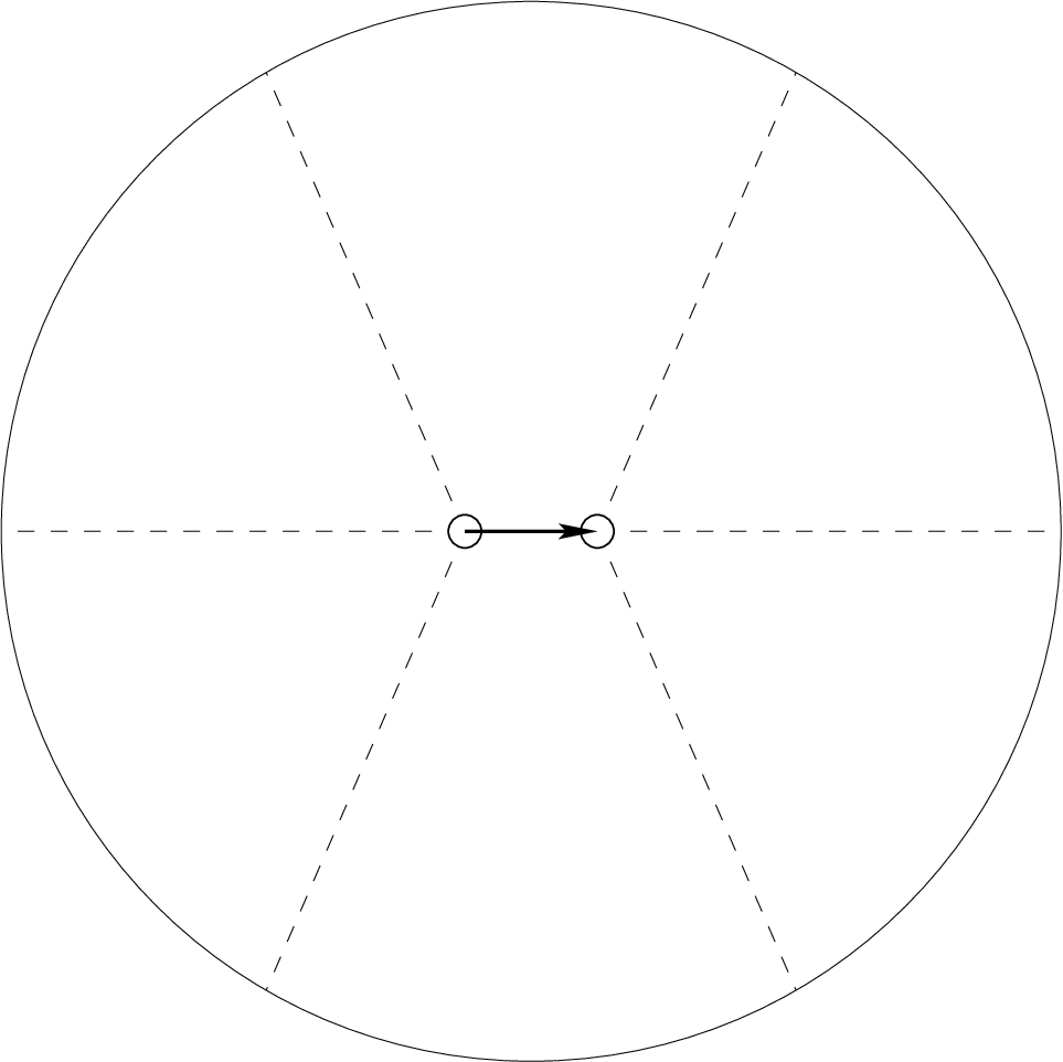

If , the number of ways of effecting the breakup is . However, we have for only half of the resulting surfaces, i.e. for ones; for another surfaces we have . If the number of the resulting surfaces is . For every such surface there are two ways to assign “names” to the newborn zeroes of order . This doubles the number of resulting surfaces with “named” zeroes. However, we again have only surfaces with ; for another ones we have . We again choose only those surfaces for which we have .
By convention we let the curve which had the endpoint at (if it was present) keep the corresponding endpoint at during the deformation. The fact that this construction was local means that except for the curve (if it exists) the holonomy is preserved along the homology basis of . The holonomy of is changed by . Furthermore every saddle connection other than has length at least .
We denote the assignment by
We denote by the stratum which contains the resulting flat surface . By construction the partition is obtained from the partition by replacing the entry by two entries and .
Recall that all the zeroes on the surface are “named”. For all the zeroes on the new surface different from the zero which was just broken we keep the same “names” on as their initial “names” on .
8.2. Collapsing a Pair of Zeroes, Principal Boundary
Now conversely, suppose we have a surface , a saddle connection of length joining distinct zeroes of orders and with holonomy , and no other saddle connection of length smaller than . Let be the other zeroes. Choose a basis of cycles in the relative homology group . This basis can be represented by a collection of curves on the surface . One of these curves, is the saddle connection joining and . If these are the only zeroes, then we can choose a basis of cycles in such way that all other cycles are closed and miss and . If there are other zeroes, then a single curve intersects one of the , say . The curve is not closed; it has as an endpoint.
One can now exactly reverse the breaking up procedure to collapse the saddle connection of length to a zero of order to construct a flat surface . Namely, we can describe a neighborhood of the saddle connection as a union of half discs of radius glued along pieces of their boundary. Two of the half discs are glued along segments of length to form the saddle connection. This leaves a pair of segments of length on each side. The other discs have marked segments of length and which are glued isometrically to form the neighborhood. We deform in the neighborhood by taking half discs of radius and gluing them cyclically along segments of length . The saddle connection is collapsed to a point which becomes a zero of order . We may perform this deformation while keeping the flat structure in the complement of the neighborhood fixed, see section 8.1 and Figures 3 and 4.
If exists then we can replace with a curve joined to . The fact that the deformation is local means that the holonomy is fixed along the entire basis other than and . The holonomy of is changed by adding . Furthermore, every saddle connection on has length at least . All named zeroes on not affected by the collapse are given the same names on . We may think of this surgery as of a Whitehead move on the foliation in direction . The resulting surface belongs to a stratum . By construction the partition is obtained from the partition by replacing the pair of entries by the entry . The stratum is in the closure of inside the moduli space of all flat structures on the surfaces of genus . We say that is the principal boundary of corresponding to this configuration.
Now choose a simply connected subset of of full volume and remove the set of flat surfaces with a saddle connection or closed geodesic of length at most . Call the resulting set . By Lemma 7.1
Choose a homology basis that is valid for all . Thus distinct have different holonomy on some basis element. As in Section 7 for or let be the set of flat surfaces with a saddle connection of length at most joining the named zeroes and no other saddle connections of length smaller than ; the configuration corresponds to a single saddle connection. We have
Lemma 8.1.
For a vector in of length at most , except for a set of of volume , there are precisely surfaces in that are the result of the assignment . Moreover, every surface in is the result of such an assignment.
Proof.
We have addressed every issue except the statement that there are precisely surfaces obtained as the result of the assignment. Suppose that for fixed two of the surfaces built from are isomorphic. Since by construction each of these surfaces has a single short saddle connection, the isomorphism sends the newborn saddle connection on one surface to the newborn saddle connection on the other surface. Hence, it sends the corresponding “disc” on one surface to the corresponding “disc” on the other surface, see Figure 4. Hence, it is an isomorphism of the complements of the “discs”, which implies that it induces an automorphism of the surface . It is sufficient to note that the set of flat surfaces, that have automorphisms, has measure . ∎


Remark 8.2.
Note that the cohomology class together with determines an element of the relative cohomology group . The lemma above claims, actually, that the local mapping is a ramified covering of order almost everywhere and that .
8.3. Computing the Siegel—Veech Constants
In this section we derive formulae for the constant in quadratic asymptotics of the number of saddle connections joining a zero of order to a zero of order in multiplicity one. According to Proposition 3.3 this means that we have to find the asymptotics of , where the configuration corresponds to a single saddle connection. Recall also that we are assuming that the zeroes are named. Since we may have numerous zeroes of orders and we, actually, have two different counting problems:
Problem 1. Count the constant in the quadratic asymptotics for the number of saddle connections joining a fixed zero of order to a fixed zero of order . (When we require that .)
Problem 2. Count the constant in the quadratic asymptotics for the number of saddle connections joining some zero of order to some other zero of order . (This is, in fact, equivalent to counting the saddle connections joining unnumbered zeroes.)
Let us start by assuming that is connected. The case of strata that are not connected will be postponed until the end of the section on higher multiplicity.
In the computations to follow we will obscure the distinction between as a saddle connection in the configuration and its holonomy. Thus we will use as a vector in the disc and as a variable of integration.
Again let , . Then . Recall that is the natural measure on . For we set where so . Then by Remark 8.2,
By Lemma 7.1
so by Lemma 8.1
Since we have
Thus, the constant from the Problem 1 has the following form:
Note that having solved the Problem 1 we get a solution of Problem 2 by an elementary combinatorial calculation. Let be the number of zeroes of order in the stratum . If , then there are ways of choosing the zero of order and ways of choosing the zero of order . Thus we get an additional factor in comparison with Problem 1.
Formula 8.1.
The constant in any connected stratum for the number of saddle connections of multiplicity one joining two zeroes of orders is equal to
| (17) |
If , then there are ways of choosing an unordered pair of zeroes of order . Having chosen an unordered pair, we choose, which of two zeroes would called be , and which one would be in arbitrary way: the number of saddle connections is obviously symmetric with respect to interchange of the names . Thus, when the answer to Problem 2 is given as the answer for Problem 1 multiplied by an additional factor .
Formula 8.2.
The constant for the number of saddle connections of multiplicity one joining two distinct zeroes of the same orders is equal to
| (18) |
Note that we may view the entire combinatorial calculation in terms of the naming of the zeroes. We can assume that on we have broken up the zero of order at the first “named” zero of order . The remaining zeroes are then given the same names on . Other zeroes of orders already have names on . There are ways of adding additional names to zeroes of orders if and if .
Note that in the consideration above the stratum might be nonconnected. In this case is the sum of the volumes of connected components. For example if we start with the stratum , then has three connected components and , and the sum of the volumes of these must be in the numerator.
8.4. Examples: Constants for Connected Strata in Genus
As an illustration of the formulae above we now give the explicit values for these constants in a number of cases.
In Table 1 we present the normalized volumes of the strata with numbered zeroes, see [EOk], see also some values in [Zo]. These values will be used for computations in all the examples.
Both strata in genus are hyperelliptic; they will be treated later on in section 10. In genus there are three connected strata: , and .
Example 8.3.
Stratum After collapsing zeroes we obtain a flat surface , where both components and occur. We have , thus the combinatorial factor equals . We get
Example 8.4.
Stratum There are two cases here in multiplicity . The first case is a saddle connection joining the zero of degree with any of the two zeroes of degree . Collapsing the zeroes we obtain a surface . For , , , . Thus the combinatorial constant equals . We get
The second case consists of collapsing the pair of simple zeroes to a zero of order . We obtain a surface . Any surface in any component of can be found by collapsing a pair of simple zeroes in this manner. Here and so the combinatorial constant is . We get
8.5. Constants for the Principal Stratum
The surface of genus has simple zeroes; . The corresponding surface has simple zeroes. The factor gives , and the factor gives . Applying formula (18)) we get
Formula 8.3.
The constant for the number of saddle connections of multiplicity one joining two distinct zeroes is equal to
In the table below we present some values of the constant in this case.
9. Multiple Homologous Saddle Connections. Connected Strata
9.1. Principal Boundary
Consider a surface with a fixed pair of zeroes and of orders and correspondingly. Suppose that we have a configuration (see Section 3) of precisely homologous saddle connections joining to of length at most . Assume there are no other saddle connections shorter than . A pair and bounds a surface . The surfaces and share the saddle connection . By convention the cyclic order of at is clockwise in the orientation defined by the flat structure. The angle between and at is ; the angle between and at be .
Cut the surface along all , . Gluing together the two sides and of the boundary of we get a flat surface with two distinguished zeroes of orders and correspondingly joined by a saddle connection, . When one of is equal to zero the corresponding point is just a marked point. If , then both points are marked points.
By construction any resulting flat surface has a saddle connection shorter than joining the pair of zeroes and does not have any other saddle connections homologous to it. Every other saddle connection is longer than . This implies that contracting the saddle connection to a point, see section 8.2, we get a flat surface with a distinguished zero (marked point) of order and no saddle connection shorter than .
Let . We say that is the principal boundary of this configuration. Note that if we mark corresponding point on , so collection contains in this case. We use the notation , see Convention 5.
9.2. Slit Construction
We would like to reverse the above degeneration and build surfaces with multiple homologous saddle connections out of surfaces in . We need the following construction. Let be a surface with a zero of order . Suppose there are no saddle connections of length shorter than . Let such that . Let be a vector of length at most . If we may break up the zero of order into zeroes of orders with a saddle connection determining joining them, see section 8.1. If take a point of the form (this means along a geodesic from in direction and distance ) and join it to on . If we take a segment from to on .
In either case we may slit the resulting surface along the saddle connection joining the two zeroes . In this way we build a surface with one boundary component consisting of two arcs, denoted and , joining the endpoints of the slit. The angles between and at the points and are and correspondingly.
Note that the flat structure on fixes the choice of the orientation. By convention we give the “names” and to the arcs in such a way that turning around in a clockwise direction from to we do not leave the surface.
Conversely, consider a flat surface with a single boundary component consisting of two arcs joining a pair of vertices. The convention on the choice of the “names” and means that as soon as we know which of two vertices is , and which is we can determine which of two arcs is , and which is .
We describe now how to build surfaces with multiple homologous saddle connections using the slit construction.
9.3. Building Surfaces With Multiple Homologous Saddle Connections
Suppose is a disconnected flat surface and on each there is a zero or a regular point which we think of as a marked point of order . Assume no surface contains a saddle connection shorter than . Given pairs with , and a vector of length smaller than , we perform the slit construction on each surface. We obtain surfaces with one boundary component each of which consists of two arcs and . We glue to , calling this curve , (and to ). This gives a closed surface , a pair of zeroes and of orders and , where and , and a set of homologous curves , joining to . The angle between and at is and the angle between them at is . We denote this assignment by
The resulting surface has no saddle connections shorter than other than the . Our convention on the choice of (see the section above) implies that the cyclic order is clockwise at with respect to the orientation defined by the flat structure.
Fix a basis for the relative homology on each surface . A relative homology basis for is given by:
- •
A relative homology basis of curves for .
- •
A curve connecting the two zeroes. The integral of along this curve is .


We introduce as from which we remove .
Having a collection of integers we denote by their sum, say, .
The construction above implies the following conditions on partitions and the numbers .
Lemma 9.1.
An assignment satisfies the following necessary conditions on the collection :
Moreover, when the stratum is connected, these conditions are sufficient: every surface with a configuration of homologous saddle connections joining the pair of zeroes of length at most and no other saddle connection with length smaller than can be obtained by an assignment with appropriate .
We shall introduce notation to describe the degeneration pattern for the surfaces .
Notation. The integer represented as a sum of two integers corresponds to represented as . Here the order of appearances of the summands is significant. The cyclic order of the surfaces is represented by .
Example 9.2.
Let ; ; . There are possible pictures for the three homologous saddle connections joining the zero of order to the zero of order depending on the returning angles (Table 3). Thus for example, the first line in table 3 refers to surfaces in cyclic order. The first is a torus (no zeroes) where we have broken up a marked point into ; the second surface has a single zero of order which we have broken into two simple zeroes indicated by , and the third surface has zeroes of , where we have broken one of the simple zeroes into a simple zero and a zero of order .
9.4. Stratum Interchange and Symmetry
In this section we discuss the possible symmetries of the assignment
Let us first specify our problem.
Problem 1. We assume that the zeroes of the surface are numbered. We fix the zeroes , , of orders and correspondingly.
We start with the case when we fix also the following data. We assume that the zeroes belong to , the zeroes belong to , …, the zeroes belong to . Here if and when and for , , when , and , when . We have .
In this setting the only thing that is not determined is the case when has exactly two zeroes: and . Then every either has a single zero of order or it is a torus with a marked (regular) point. Note that we fix only the cyclic order of the collection , but not the numbering of each of these pair of numbers. The natural action of the cyclic group of order on the collection of ordered pairs organized in a cyclic order, may have nontrivial stabilizer, which we denote by . We get symmetry of order . This type of symmetry we call the stratum interchange.
Problem 2. Now consider the problem with fewer constrains. We count the number of occurrences of the following phenomenon: some zero of of order is joined to some zero of order by precisely homologous saddle connections as above. We fix the type of the flat surface obtained as described above, but we make no assumptions on the distribution of the zeroes by the surfaces . As before we fix only the cyclic order of appearances of the surfaces .
Remark 9.3.
Problem 2 may be considered as generalization of Problem 1 to the case when the zeroes of and of are not numbered.
Remark 9.4.
In both settings the might be nonconnected. We could also specify the connected component of the when this occurs. We prefer the setting where this data is not specified.
Consider the natural action of the cyclic group of order on the collection
organized in a cyclic order. (Recall the notation from the previous section). If it has a nontrivial stabilizer we denote it by the same symbol . We get a symmetry of order which we also call the stratum interchange.
Example 9.5.
Let , , . Consider the degeneration of into surfaces of the following types
The possible symmetry in this case is a symmetry of order , where subgroup is a shift by .
The degeneration
possesses this symmetry, while the degeneration
does not.
When we may have an additional symmetry in Problem 2. Let be two zeroes of of order joined by precisely homologous saddle connections. Let the homology class of the saddle connection be represented by a vector . Assigning the “names” and to and we get a decomposition .
Consider now the very same surface with the same configuration of homologous saddle connections joining the same two zeroes and . We may declare now that the correspondence of zeroes is inverse with respect to the previous assignment: and . Since our saddle connections are oriented (from to ) the homology class of the same saddle connection (from to ) is represented now by the vector . Since the cyclic order of “pieces” is determined by the cyclic order at the point the new identification reverses the cyclic order in the collection , as well as the order in the pairs .
We say, that we have a symmetry if and only if the assignment and gives a decomposition with the same (up to a cyclic reenumeration) collection as before.
It is easy to see the following combinatorial criterion of the symmetry. Interchange simultaneously all , and change the cyclic order of the resulting collection to the opposite one. We possess a symmetry if and only if the result of this operation gives us the initial collection up to a cyclic reenumeration. We denote symmetry by , where . We let when there is no symmetry.
The condition is an obvious necessary condition for symmetry. It will be always assumed in the discussions of symmetry.
Under this condition every degeneration of multiplicity
possesses a symmetry. There is a
symmetry in multiplicity if and only if at
least one the following conditions is valid: either
— (and then automatically);
or
— and (and then
automatically).
Example 9.6.
Let . Consider degeneration of into surfaces of the following types :
The degeneration
possesses the symmetry, but does not have the stratum interchange, so , .
The degeneration
does not have a symmetry, but allows the stratum interchange, so , .
The degeneration
has both symmetries: , .
Remark 9.7.
Describing the assignments one can consider all possible assignments, and then take into account corresponding symmetries, or one can deal with the classes, eliminating the symmetry whenever it is possible.
We have chosen the second way. For example the assignment
is not presented in the Table 3 since it is symmetric to the assignment
(which is in the list) by composition of symmetry with the stratum interchange.
Let us return to the degeneration construction described in Section 9.1. To every surface in the thick part we associate a surface . We denote the corresponding stratum by , where , see Convention 5.
However, our consideration of the symmetries shows, that the surface is defined up to a finite symmetry. In other words, we may have a nontrivial symmetry group acting on the stratum . This symmetry group is generated by the subgroup of stratum interchange symmetries and subgroup of symmetries. (Any of the subgroups, or both might be trivial.) The order of the symmetry group is equal to the product of the orders and .
Note that the symmetry group preserves the natural measure on . It obviously preserves the area of the surface, hence preserves the “unit hyperboloid” . Thus we get a natural volume element on the quotient .
The degeneration construction can be considered as a map
In the next section we shall study this map. This will allow us to compute the volume of the thick part and thus compute the corresponding Siegel—Veech constant.
9.5. Siegel—Veech Constants in Higher Multiplicity, Connected Strata
Consider the set . It consists of surfaces having exactly one collection of short homologous saddle connections. This collection is necessarily of the type ; the saddle connections from this collection (which are all of the same length) are shorter then ; any other saddle connection on is longer then .
Actually, we shall need two variants of this set: the one, which we denote corresponds to the value of parameter ; the other, denoted , corresponds to .
Clearly,
| (19) |
Lemma 9.8.
Consider the map
corresponding to the assignment . Let
1. The image of the map contains the subset .
2. Let . The restriction is a (ramified) covering of degree
| (20) |
where is the degree of the distinguished zero on the surface .
3. The map is volume preserving: the volume element on induced from on coincides with the volume element on .
4. The set contains the set .
Proof.
In fact, the statement of the Lemma is almost tautological reformulation in geometric terms of the properties which we already know.
Part 1 follows immediately from the construction in the beginning of Section 9.3, where having a surface and a vector we constructed a surface . We have .
The fact that is nondegenerate almost everywhere follows immediately from consideration of in cohomological coordinates, so in this sense it is a (ramified) covering. To prove statement 2 it remains to compute the degree of this covering, i.e. to prove that for almost all pairs we can construct exactly pairwise nonisometric surfaces. For each surface there are ways to perform a slit construction at a zero of order of providing surfaces . According to Lemma 8.1 for almost all the resulting surfaces are pairwise nonisometric. For almost all the surfaces and corresponding to different indices are nonisometric as well. Thus generically there are no isomorphisms between the resulting surfaces which map the collection on one surface to the collection on the other surface. Since by the choice of such a collection is unique on each of the surfaces , they are generically pairwise nonisometric.
Statement 3 follows immediately from the fact that as a basis of cycles in we can choose a union of basic cycles for and one of the homologous saddle connections , where by definition . Thus, this statement is completely analogous to the corresponding statement in multiplicity one.
Statement 4 follows from the fact that the surgery, which associates a surface to a surface either does not change the holonomy of saddle connections different from or changes it by holonomy of . Since it means that a saddle connection, which is longer than would stay longer than after the surgery. ∎
Corollary 9.9.
Suppose that the stratum is connected; let be an admissible configuration of saddle connections joining a pair of distinct zeroes; let be the corresponding assignment. Then
where the integer constant is defined as
| (21) |
Here ; if the assignment has symmetry and otherwise; is the order of the “stratum interchange” symmetry.
Proof.
Combining statement 4 of the Lemma above with the obvious inclusions (19) we obtain the following inclusions
Hence, by Corollary 7.2
On the other hand, by statements 2 and 3 of the Lemma above,
The volume of the disc equals . The volume of the quotient over a finite group of isometries equals to the volume of the total space divided by the order of the group. Since , and the set is defined as
we obtain
It follows from Lemma 7.1 that . Hence,
Summarizing the above arguments we obtain the statement of the corollary. ∎
Now everything is ready to compute the Siegel—Veech constant . Note that we work in the setting where we fix the partition of numbered zeroes of by components (see Problem 1 in section 9.4). We assume that is connected. Applying Proposition 3.3 we get the following value of the :
Using expression (21) for and Formula (12) from Section 6.2 for the volume of a nonprimitive stratum we finally obtain the following formula:
where
| (22) |
Note, that if , the corresponding surface has a marked point, so contains . Note also, that by convention when is a torus, we use the point which is already marked, so .
Let us study now the constant in the setting where we do not specify which zeroes are to be joined. (see Problem 2 in Section 9.4). This counting problem can be reduced to the previous one by a purely combinatorial computation. Consider , , , . Then these zeroes are all “inherited” by the surfaces . Since all the zeroes are named, the number of ways to distribute zeroes of order into groups of zeroes equals
If and but for some then one of the zeroes of order which lives on is newborn; that is, arising from the degeneration, while the other zeroes of order come from the corresponding zeroes of order on . Thus the corresponding factor in the denominator becomes . Multiplying numerator and denominator by we get the following factor:
(Equivalently, we may say that we have performed the slit construction at the first “named” zero of order on . The rest of the zeroes of that order inherit their names on , but then we count the number of ways of merging the names from different onto .) Consider now the case when or . When and (resp. ) we have the arrangements of the other (resp. ) zeroes of order . When we have an arrangement of the other zeroes of order . This changes the numerator in the formula above by the corresponding factorial. However, in these cases we have to count the number of ways to choose a zero of degree and a zero of degree on the initial surface . This number is equal to if and if . Thus for zeroes of these degrees we have this extra factor which combined with previous considerations gives in this case as well. Taking into account the possible symmetries (see section 9.4), we finally get the following expression for the constant in the setting where the zeroes of are not numbered (see Problem 2 in section 9.4).
Formula 9.1.
| (23) |
We give some examples of this formula in the case of connected strata .
Example 9.10.
Stratum ; The multiplicity is . After degeneration we get a surface of genus with a single zero of order , where now , and we get a torus , with .
The saddle connections and partition the cone angle at in two sectors with angles and ; they partition the cone angle at in two sectors with angles and . There is no stratum interchange, so . We get
Example 9.11.
Stratum ; genus , multiplicity . First suppose that we have a pair of homologous saddle connections joining the zero of degree with one of two zeroes of degree . After degeneration we get two surfaces , and , where . Thus , . There is no stratum interchange, so . Altogether we get
Suppose now that we have a pair of homologous saddle connections joining two simple zeroes. After degeneration we get two surfaces , and , where . Thus is genus with a marked point and with a zero of degree , while is a torus with a marked point. Here we have , .
There is no stratum interchange, so . We now get
9.6. Principal Stratum
The cone angle at any simple zero equals . Thus for the principal stratum we may have at most two homologous saddle connections joining a pair of distinct zeroes. Hence in the higher multiplicity case, the surface of genus degenerates to a pair of surfaces of genera . Each of has only simple zeroes and one additional marked point. We always have the symmetry, so . When we have a symmetry due to the stratum interchange; there is no other symmetry otherwise.
Formula 9.2.
The constant for the number of saddle connections of multiplicity two joining two distinct zeroes in the principal stratum is

Table 4 presents the numerical values for these constants. More values are presented in Table 8 in the Appendix. (We present only approximate values of constants in Table 8 just to save the space.)
10. Strata Having Several Connected Components
The analysis of admissible assignments, structure of local surgeries, and most of the elements of our constructions are basically the same for the strata having several connected components. However, we need to establish the correspondence between connected components and parts of the boundary of the stratum they are adjacent to. In other words we need to describe the admissible constructions, which lead to the flat surfaces in the prescribe connected component.
10.1. Parity of the Spin Structure in the Slit Construction
We start with outlining the relation between the parities of spin structures of the resulting surface and its components in the slit construction.
Lemma 10.1.
Suppose constructed above has only even zeroes so has a spin structure. Then each component surface has only even zeroes and so also has a spin structure. The parity of the spin structure is equal to the sum of the parities of the spin structures of the components:
| (24) |
Proof.
For each , all the zeroes except the distinguished one come from the corresponding zeroes on unchanged; in particular they have the same degrees as the initial zeroes of . Thus for each all the zeroes but at most one, have even degrees. Note that the total sum of the degrees of the zeroes of is even: it equals , where is the genus of the surface . Hence the remaining zero has even degree as well. (By usual convention we consider a marked point as a “zero of degree ”.)
For each surface consider a collection of smooth simple closed curves on representing the canonical basis of cycles. Breaking up the zero we make a local surgery of the flat structure, i.e., we do not change the flat structure outside of a small domain containing the zero . Thus for each we can deform if necessary the curves from the corresponding collection in such a way that they stay outside of a neighborhood of the zero . Thus we may assume that for each none of the chosen curves on intersect . This means that all the curves survive under the surgery, moreover, the union of collections for all gives us a canonical basis on . By construction the index of any resulting curve in the flat structure is the same as the index of the corresponding curve in the flat structure . Hence we get the desired relation (24). The lemma is proved. ∎
10.2. Admissible Assignments for Surfaces from Hyperelliptic Components
Note that the surfaces from the hyperelliptic component and from the hyperelliptic component , where is odd, also have parity of the spin structure (see formulae (8), (9)). In general these surfaces are also involved in assignments from Lemma 10.2 producing nonhyperelliptic components and . However, in the exceptional case of with odd some assignments lead to surfaces from the hyperelliptic connected component . These assignments are classified in the lemma below.
Lemma 10.3.
Let a flat surface from the hyperelliptic connected component be obtained by an assignment
Then for almost every the assignment has one of the following two types:
- —
The multiplicity is ; the flat surface belongs to the hyperelliptic component , and .
- —
The multiplicity is ; the flat surfaces , belong to the hyperelliptic components , where , and , .
The assignment is to and is onto the corresponding set of hyperelliptic surfaces.
Proof.
The set of hyperelliptic structures such that the involution interchanges some components has positive codimension, so we may disregard these and assume the involution fixes each component. This implies that all flat surfaces belong to components . Since the hyperelliptic involution sends a vector to , but does not change the orientation of the surface, if the multiplicity is greater than one, it cannot map any of the or to themselves. It must therefore interchange and for each . This implies that . ∎
Corollary 10.4.
Almost any flat surface from the hyperelliptic connected component has no saddle connections of multiplicity greater then two.
10.3. Constants for the Components of the Stratum
We start with the stratum which is exceptional: it has the hyperelliptic connected component.
10.3.1. Hyperelliptic Connected Component
The admissible assignments for the surfaces from the hyperelliptic connected component are described by Lemma 10.3. The possible multiplicities are one and two. In multiplicity one modifying (18) in accordance with Lemma 10.3 we get the following formula.
Formula 10.1.
The constant for the number of saddle connections of multiplicity one joining distinct zeroes in is given by
In other words, collapsing a saddle connection of multiplicity one on a surface we get a surface from the hyperelliptic connected component . Breaking up the zero of a surface we necessarily get a surface from the hyperelliptic component .
Example 10.5.
Component . In genus the component coincides with the whole principal stratum . The formula above gives the same constant as formula 8.3 for the principal stratum in genus :
Example 10.6.
Component . In genus we have the connected component . After collapsing zeroes we obtain a hyperelliptic surface . We get
We present more values in table 5.
Consider now multiple saddle connections for a flat surface from the connected component . By Lemma 10.3 we only have in the higher multiplicity, and , , where . Here we always have the symmetry, so . When we also have the stratum interchange symmetry, so , and otherwise. Thus, after appropriate modification of formula (23) we get the following constant
Formula 10.2.
The constant in multiplicity for saddle connections joining distinct zeroes in is given by
Example 10.7.
Component . Saddle connections of multiplicity two joining distinct zeroes on a surface from were actually, already considered in the section treating the principal stratum. Here after decomposition we get a pair of tori each with a marked point. We get the following value for the corresponding constant:
Example 10.8.
Component . Consider saddle connections of multiplicity two joining distinct zeroes on a surface from . After decomposition we get a surface of genus with a single zero of order and a torus with a marked point. The cone angle between and is the same at and ; it equals . The cone angle between and is also the same at and , but now it equals . The constant is given by
10.3.2. Connected Component ; Even Genus
For , even, the stratum has exactly two connected components: and . Thus, dealing with the connected component we have to exclude all the assignments producing surfaces in the stratum those that actually belong to the component . The latter problem has already been solved. Thus we get the following answers.
Formula 10.3.
For any even genus any flat surfaces from the connected component having a saddle connection of multiplicity one joining distinct zeroes may be obtained from the corresponding surface from one of the components , .
The corresponding constant is equal to
We proceed with multiplicity two. Here we get the formula analogous to formula 10.2 for the component .
Formula 10.4.
The constant for multiplicity joining two zeroes in the stratum is given by
For multiplicity it is easy to account for the impact of the hyperelliptic component (see Corollary 10.4). We get the following particular case of formula( 23) in the case of
Formula 10.5.
10.3.3. Components and
We consider the multiplicity one case first. Assume that belongs to one of the nonhyperelliptic components or . Contracting the saddle connection joining the two zeroes, we merge the two zeroes into one and we get a surface in or correspondingly. Conversely breaking up a single zero of a surface from a nonhyperelliptic connected component or into two zeroes of degrees we get a surface from the component or correspondingly. Thus we have to modify formula (18) in the following way.
Formula 10.6.
The constant is equal to
Example 10.9.
Component After collapsing zeroes we obtain a surface . We get
Remark 10.10.
Note that the similar nonhyperelliptic connected components with even parity of the spins structure do not exist in genus .
Now we consider higher multiplicity. We again have to consider multiplicity two separately because some assignments in multiplicity two produce surfaces from the hyperelliptic connected component , see Lemma 10.1. We again get the formula analogous to formula 10.2 for the component and to formula 10.4 for the component .
It will be convenient to introduce the following notation. We introduce a function which has values or . It is equal to when all of the following three conditions are satisfied: all the zeroes of (if any) have even degrees; contains the hyperelliptic component ; the parity of the spin structure of coincides with . Otherwise .
Formula (8) for the parity of the spin structure of shows that
| (25) |
We shall also use the following convention: the volume of a nonexistent component is equal to zero. In this notation we get the following six “dummy” volumes for the strata in small genera:
| (26) |
and also we have
Formula 10.7.
A surface from one of the nonhyperelliptic connected components or may have a saddle connection of multiplicity two joining the two distinct zeroes if and only if it can be obtained from surfaces and of genus where and where the following additional requirements are satisfied. At least one of the surfaces does not belong to the hyperelliptic component , ; the parities of the spin structures of the surfaces satisfy relation (24): . For the spin structures of should have opposite parities. This means in particular that there is no longer a stratum interchange symmetry. For
For , where is even, we get
Example 10.11.
The expression for the constant for the surfaces from is analogous to the one above with the only exception that now we get the stratum interchange symmetry for :
Finally, for from multiplicity at least three it is easy to account for the impact of the hyperelliptic component (see Corollary 10.4). We get the following particular case of formula( 23):
Formula 10.8.
Almost every surface in or in having saddle connections of multiplicity joining two zeroes can be obtained by assignment
where , , and . The corresponding constant equals
Note that here we always have the symmetry, , which is cancelled by (see (23)). Note that in this particular case we prefer to use summation over all combinations of parities producing the proper parity of the sum. Thus the stratum interchange symmetry depends only on the collection of , and on their cyclic order.
Example 10.12.
Component Consider a saddle connection joining the two zeroes of a surface , and suppose that the saddle connection has multiplicity . Each of , for is a torus with a marked point. The angle between any consecutive saddle connections at and equals . There is a symmetry of order coming from stratum interchange, so . Taking into consideration from we get
Remark 10.13.
Let be odd. We see that the maximal multiplicity of a saddle connection joining the distinct zeroes of a surface from the stratum is different for different connected components: it equals for almost all surfaces from , it equals for almost all surfaces in ; it equals for almost all surfaces in .
10.4. Other Strata
The description for all other strata , where all the entries of are even, is similar to the one just presented.
Formula 10.9.
The constant for the nonhyperelliptic connected component , , , is given by
Example 10.14.
Stratum In multiplicity one, after collapsing zeroes we obtain a surface , where either of the two components and having even parity of the spin structure are possible. We get
In multiplicity two we get two surfaces , , where .
There are two possibilities. In the first case . Note that any has odd parity of the spin structure, see (8). Thus the parity of the resulting flat structure is even, see Lemma 10.1.
The saddle connections and partition the cone angle at in two sectors with angles and ; they partition the cone angle at in two sectors with the angles and . Here while so that while , there is no stratum interchange since . Thus . We get
In the second case after degeneration we get , Since has odd parity of the spin structure, in order to result in a surface (see Lemma 10.1).
The saddle connections and partition the cone angle at in two sectors with the angles and ; they partition the cone angle at in two sectors with the angles and . We get
Multiplicity is not realizable in the component (see the next subsection).
Example 10.15.
Stratum This component is similar in many aspects to the previous one, so we skip those details of calculations which are common for both components.
The first case is with multiplicity . After collapsing zeroes we obtain a surface , the only component that results is . We get
Consider multiplicity . The case of degeneration to two surfaces does not take place here, since the surface obtained from two surfaces from has even parity of spin structure.
Thus, the only possibility is ; , , . Since has odd parity of the spin structure, must be in components of having even parity of spin structure in order to result a surface (see Lemma 10.1). There is only one such component: .
Thus we get
(see analogous calculation for the component .
Consider now multiplicity . It is not hard to check that , . Note that both and have odd parity of the spin structure. Thus the resulting surface always has odd parity of the spin structure, see Lemma 10.1.
The saddle connections partition the cone angle at in three sectors with the angles , , and ; they partition the cone angle at in three sectors with the angles . We find
Part 2. Saddle Connections Joining a Zero to Itself
In this part we consider the second problem of this paper: we count closed saddle connections joining a zero to itself.
11. Approaching the Principal Boundary by Shrinking Closed Geodesics
11.1. Configurations of Closed Saddle Connections and Corresponding Surface Decompositions
We have already indicated in Section 3.2 that together with a closed saddle connection joining a zero to itself some other saddle connections homologous to might be present on a surface , see Figure 7. There might be also some metric cylinders filled with regular closed geodesics homologous to ; such cylinders are bounded by the singular closed geodesics from the collection . Suppose that the curves with indices from a set bound cylinders. The complement of the union of the curves and the cylinders splits into disjoint surfaces . For example, the surface presented in Figure 7 is composed of surfaces and of cylinders, where one cylinder joins to and the other cylinder joins to . When the boundary of the closure of any surface is a union of two singular closed geodesics .
The sum of the genera of the is . The surfaces are attached in some cyclic order. Thus, for any the “next surface” and the “previous surface” make sense mod . We use the following convention for the cyclic order: let be the vector orthogonal to and pointing from to . Then the frame corresponds to the canonical orientation of the surface induced by the complex structure.


We distinguish two types of surfaces .
If the boundary of the closure of has two connected components, we get a surface of the first type. In this case the boundary is formed by two disjoint singular closed geodesics and . The surfaces and in Figure 7 are of that type. The closed geodesics contains a single conical point the closed geodesics contains a single conical point . We denote by the cone angle at inside , and by the cone angle at inside .
Suppose now that the boundary of the closure of has a single connected component produced by two singular closed geodesics sharing the same conical point . Cut at this conical point. If the boundary of the resulting surface now has two connected components, that means that the surface is obtained from a surface described in the paragraph above by identification of the conical points , and we do not distinguish a surface of this type from those discussed above.
We also put in the first group the surface if ; that is, if we have a singular closed geodesic of multiplicity one which does not bound a cylinder of regular closed geodesics. Cutting by we again obtain a surface with two disjoint boundary components as above. The initial unique conical point produces two distinct conical points; one on each of the two boundary components.
Consider now the remaining case. Suppose that the boundary of has a single connected component produced by two singular closed geodesics and sharing the same conical point . If the boundary of the surface cut at still has a single connected component, we say that we get a surface of the second type. For example, the surfaces and at Figure 7 are of that type. The curves bound angles and inside at the conical point . The two boundary curves and are joined together at the zero forming a “figure eight”.
Therefore we get two types of surfaces ; a boundary of each surface is produced by a pair of singular closed geodesics . Altogether the configuration consists of the data
We will show how to metrically shrink the boundary components of each to produce a closed surface. For surfaces of the first type the boundary curves will shrink to zeroes of orders and for surfaces of the second type to a single zero of order . Each such closed surface will then lie in a stratum and the union of these strata comprises the principal boundary.
The goal of the rest of this section is to describe how, for each , one can naturally “shrink” the boundary components to obtain a closed regular flat surface. We start with surfaces of the second type.
11.2. Shrinking a Pair of Adjacent Holes
Suppose that the boundary of has a single connected component produced by two singular closed geodesics sharing the same conical point ; the boundary of such surface has a form of figure eight. By assumption the surface is of the second type, so cutting at we get a surface with a connected boundary. The surgery corresponding to cutting at is illustrated at Figure 10. We start with the surface presented on the right of Figure 10 (there is an extra flat cylinder drawn in the picture, this flat cylinder will be discussed later) and we get the surface presented in the middle of Figure 10. By construction, the boundary of the surface obtained after the surgery is made up of two parallel geodesic segments of the same length (coming from and ) joining two singular points (obtained by breaking into two distinct points). The cone angles inside at these points are denoted by and . Now we identify the two geodesic segments which form the boundary; see the left picture at Figure 10. We get a closed surface with a saddle connection joining the two zeroes. By construction this saddle connection has direction and length ; moreover, by construction the resulting surface does not have any other saddle connections homologous to . Thus, if the initial surface belongs to then the surface obtained from by our surgery does not have any other short saddle connections, except . Hence, following the construction of section 8.2 we can collapse the saddle connection into a single zero of order . We have proved that for any from there is a canonical way to associate to every component of the second type a closed flat surface .
In other words, we have proved that for a surface of the second type (one having boundary formed by two small adjacent holes) there is a canonical way to shrink metrically the holes, obtaining as a result a closed flat surface .
11.3. Transporting a Small Hole Along a Flat Surface
Intuitively one can interpret the surgery described in the previous section as annihilation of a “” and a “” hole which are joined together. In this section we show how one can continuously deform the location of an isolated small hole on a flat surface. In the next section we consider a flat surface with a pair of small holes located at different places on the surface. Using the hole-transport construction we move “” and “” holes in such way that they become adjacent to each other and then we make them annihilate as was described in the previous section.
In this section we consider the case of multiplicity one. Moreover, we assume that the short closed saddle connection of multiplicity one does not bound a metric cylinder. Choose some orientation of ; let . Let be the length of the shortest saddle connection different from . Assume that . Now cut the surface along . Since is not homologous to zero, we get a connected surface with boundary having two connected components. Each component is formed by a single geodesic segment containing exactly one conical point. By construction the size of the holes is small with respect to the scale of the surface , and the holes are located relatively far away one from the other.
Choose one of the holes, say, the positive one for which the orientation induced by the natural orientation of the boundary coincides with the chosen orientation of . We denote this hole as . Let be the unique singularity point located on . Consider the set of points in located at distance less than or equal to from . Denote the cone angle at by ; it is easy to see that the cone angle is always an odd multiple of , with being some nonnegative integer. The set is composed of regular sectors, isometric to metric half-discs of radius and of one irregular sector. The irregular sector can be constructed metrically as follows: superpose two copies of metric half-discs of radius ; then shift one with respect to the other by in direction of the common diameter; finally, take the union of the resulting metric half-discs; see Figure 8. The distinguished sector contains the hole, see Figure 8, so its impact to the cone angle at is instead of . We choose the boundaries of the sectors to have directions . We denote the distinguished sector by ; we enumerate the other sectors in a cyclic order.


Consider a geodesic segment having the conical point as one of the endpoints; let be the other endpoint of ; let be the length of . We assume that , so is located in the interior of . Our goal is to “move the hole” to the point . We treat separately the four cases listed below which describe all possible locations of . Each time we modify some sectors or the identification of the boundaries of the sectors in such way that after regluing of the modified sectors a neighborhood of the boundary of the modified domain stays isometric to a neighborhood of the boundary of the initial domain . In this way we can cut out of the flat surface; make a surgery on and then metrically paste back the modified domain into the surface. Here is a complete list of possible locations of (see also Figure 9); as usual indices are taken modulo the largest one, so .


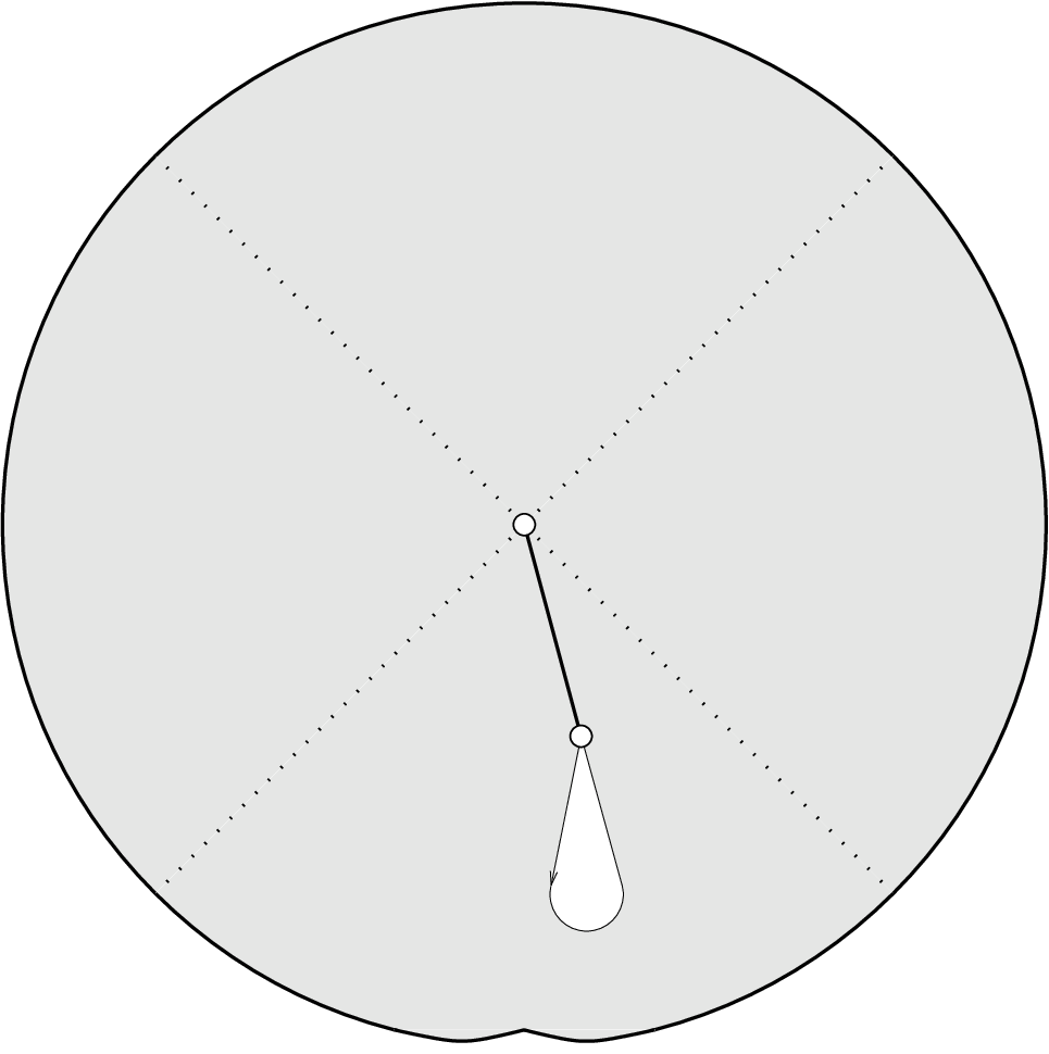


I. and has direction ;
II. and has direction different from ;
III. and has direction different from ;
IV. and
- I.
and has direction ;
- II.
and has direction different from ;
- III.
and has direction different from ;
- IV.
where
I. Moving the hole along .
To move the hole in direction
it is sufficient to modify the identification
of the boundary of with the boundary of .
Similarly, to move the hole in direction
it is sufficient to modify the identification
of the boundary of with the boundary of .
The first case is illustrated at
Figure 9, case I. We identify
the segments on and on
(this is exactly
our geodesic segment of length ). Then we leave
a segment of length on
without identification, but we identify its endpoints
getting a single point .
This is the new hole. Then we identify the remaining segments
of length (the ones to the right of the point
at Figure 9, case I)
on and on .
In other words, our surgery consists of marking a superfluous segment of length on the boundary of at the distance to the right (correspondingly to the left) of the initial location.
II. Moving the hole inside the distinguished sector.
Consider a parallelogram in having and
as a pair of sides (see Figure 9, II);
let and be the other two sides of parallel to
and correspondingly. We can think of as of a
parallel translation of by . Cut out of and identify
the opposite sides and in .
Perform the initial identification of the boundaries of the sectors using instead
of . As a result of this surgery we get a new domain
with a hole located at the point . Note that
performing this surgery we have reduced the area of the surface
by the area of the parallelogram which was cut out.
III. Moving the hole inside one of the two adjacent sectors
.
If the segment transversal to the direction
is located in one of the sectors , we can
perform an operation inverse to the one presented above.
Suppose that, say, .
Consider a parallelogram in the Euclidean plane
with a pair of sides having the same lengths and
directions as and correspondingly.
Slit along from to ;
let and be the sides of the resulting slit. Identify
the corresponding sides of with and . We have
modified the sector in the following way: the
modified sector has an extra segment at the base,
where , and a new hole at the point ,
where .
Perform the initial identification of the boundaries of the sectors using instead
of ; add a new one identifying the segment of length
at the base of
with the segment of length at the base of .
As a result of this surgery we get a new domain
with a hole located at the point . Note that
performing this surgery we have increased the area of the surface
by the area of the parallelogram which was pasted in.
IV. Tunnelling the hole to a nonadjacent sector.
If the segment
is located in a sector where we first “push
the hole” either to or to its neighbor. This reduces
the situation to one of the cases I–III.
We push the hole to the sector ,
where if is even and if is odd. To do this
we change the identifications of the boundary segments of the
sectors as indicated at
Figure 9, case IV.
The operation of
tunnelling the hole to a nonadjacent sector does not change the
area of the surface.
11.4. Shrinking a Pair of Nonadjacent Holes
To simplify the construction above we assumed that the path , along which we have transported the hole, is a geodesic segment which is shorter than the shortest saddle connection. It is quite clear how to generalize the construction in several ways.
A geodesic segment transversal to can be replaced by a path transversal to ; the result of the surgery depends only on the homotopy class of , where the homotopy is performed with the fixed endpoints; the path remains transversal to during the homotopy; the homotopy is performed inside the surface with punctured singularities.
We can invert our construction: having a hole located close to a zero we can move it to the zero.
The segment (path) need not be necessarily short: an appropriate surgery can be performed using a finite covering of by domains . However, we require that is either a segment parallel to or a segment (path) transversal to . We also require that does not have self-intersections, and, moreover, that it does not make “almost loops” when a pair of points located far one from another with respect to parameterization of by length occur to be close to each other on the surface.
Finally, we can consider a situation when is a broken line of geodesic segments joining singularities . We can consecutively move the hole along the first segment from singularity to singularity ; perform if necessary tunnelling of the hole from one sector at to another; move the hole along the second segment from singularity to singularity ; etc, and finally bring the hole to the appropriate sector of .
We can now return to our original problem. We have a surface with two small holes which we want to shrink metrically. We move one hole to another and then apply the construction of shrinking a pair of adjacent holes.
Note that the operation of moving a hole from to typically changes the area of the surface. However, the change of the area is at most the product of the length of circumference of the hole by the length of the path .
12. Constructing Surfaces with Homologous Closed Saddle Connections
Our objective now is to reverse the shrinking operation to show how to build homologous saddle connections with associated configuration out of simpler surfaces. We shall start with a collection of closed surfaces and via a “figure eight” and “creating a pair of holes construction” build a closed surface with a curve or set of homologous curves joining a zero to itself.
Fix and let denote a compact simply connected subset of such that for every saddle connection has length at least . By Lemma 7.1 its complement has volume . Choose a homology basis that is valid for all .


12.1. Figure Eight Construction
Given a surface , a zero (or a marked point) of order , and a pair of numbers we may break up the zero and perform the slit construction. We may then identify the two endpoints of the slit. This gives a surface with two circular boundary components , which are joined at a point, see Figure 10. The two circular boundary components separate the total angle at the point into angles and . By convention on the choice of (see Section 9.2) turning around in a clockwise direction from to inside the surface we turn by the angle .
Recall that we may break the zero of order up in ways. Thus the figure eight construction is not uniquely defined; the construction gives surfaces.
12.2. Creating a Pair of Holes
In this construction we are given a pair of distinct points and a vector. We shall “open” the surface at the two points using the vector to build a surface with two boundary components. The construction depends on choosing a path between the two points, and so is not quite canonical. Suppose then that and are zeroes of orders on a surface , is a vector of length . Let be the shortest path joining and . It consists of saddle connections. On a set of surfaces of full measure none of the saddle connections are in the direction . The endpoints of the segments are located at conical points. We need first to estimate the length of and establish a few simple properties of the path. We use Corollary 5.7 from paper [MS] (in which we adjusted the notations).
Proposition (H. Masur, J. Smillie).
Let be a closed flat surface with diameter . Let be any geodesic segment joining singularities whose length is minimal among all geodesic segments that join singularities. Assume that is not a simple closed curve which bounds a metric cylinder. Let be the length of the shortest geodesic element joining singularities not equal to . Then there is a constant depending only on the genus of the surface such that .
From the assumption on , and the above Proposition for a new constant . Since is a shortest path it does not have any self-intersections, so a conical point may have at most two segments of adjacent to it. If comes within of a singularity other than at its endpoints, we may modify choosing a broken line going through that singularity, increasing the length of by at most . Since the shortest loop on the surface has length at least , and there are at most conical points, for small , after at most replacements we can assume that the new path does not pass within of any singularity except at its endpoints. The total increase in length is at most and so its length is bounded by for a slightly different . (The path might now be not shortest.)
Proposition 12.1.
- (1)
Any line segment of length in direction through any point on does not meet again.
- (2)
For small and any saddle connection , the algebraic intersection .
Proof.
To prove (1) notice that if the intersections points of the line segment with were further than apart on , we could shorten by more than following the line segment between and instead of , which is impossible. If are within of each other on we have a loop of length at most for small , which is also a contradiction.
The proof of (2) is similar. ∎
Now returning to the problem of creating a pair of holes, suppose we are given a pair of separatrices leaving and in direction . The notion of as the point makes sense for small . Perform the figure eight construction using the points and creating a surface with a pair of holes joined at a point .
We can now transport a hole from to along as was described in the previous section. Conclusion 1) of the Proposition says that the hole transport is well-defined. We get a surface with two holes. We may then tunnel the hole at so that it is adjacent to the given separatrix. Note that the operation of creating a pair of holes typically changes the area of the surface. However, the change of the area is at most the product of the length of circumference of the hole by the length of the path . Our estimates show that the change of the area is bounded by .
We note that the resulting flat structure depends on the choice of the separatrices leaving each zero, on the homotopy class of the path as well as on the other given data. From (2) we see that for any saddle connection , the length of on the new surface is at least and since on , on the new surface must have length at least .
12.3. Admissible Constructions
We formalize the above construction as follows. Consider the following data:
- •
For : surfaces with and no saddle connections shorter than
- •
A vector , with .
- •
For : a pair of points which are zeroes of orders or marked points. The points may coincide. If they are distinct, we are also given a broken line joining and . For any including those in a fixed homology basis,
(27) where is the algebraic intersection number.
- •
, where is a constant.
- •
If is a zero of order , then a pair of numbers with .
- •
A subset , where . By convention, when we let .
- •
For : a number such that .
- •
For : a number with .
Given the above data we construct a flat surface with homologous saddle connections of multiplicity with associated data . Namely, for each , if we use the figure eight construction and if we use the construction of creating a pair of holes giving two boundary curves and . For each either glue directly to or, if glue in cylinders of “width” , “height” and “twist” to connect to ( considered mod ).
The resulting surface also depends on the data and . Denote by the union of the pieces , the vector of , the vector of and the collection of . Then we have an admissible construction
A relative homology basis for is given by:
- •
A relative homology basis of curves for each component of .
- •
If one of the is a marked point, the curve . If both are marked points, then in addition to a curve from some singularity on to (or to ) unless is a torus.
- •
A closed curve in the homology class of . The holonomy along this curve is .
- •
For each cylinder a curve joining its boundary singularities. The holonomy of this curve is .
We summarize the discussion as follows.
Lemma 12.2.
Suppose that we
— either use at least one construction of creating a pair of holes;
or
— if we use only figure eight constructions, we use at least
one cylinder.
Then the resulting surface is a nondegenerate flat surface with no saddle connections other than the shorter than and thus it lies in .
The holonomy vectors on of those curves , which correspond to the original homology basis on are given by
| (28) |
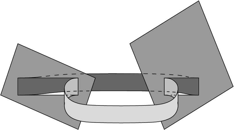
Example 12.3.
In the example presented at Figure 11 we take two flat tori. In the picture they are represented by the large parallelograms with identified opposite sides to , to , and to , to . In fact, the zeroes , , and , are fake here: all these points are just marked points of the tori. In this example we choose the vector to be vertical.
We cut a rectangular domain out of the interior of each of the two tori in such way that the vertical side of each of the two removed rectangles is equal to . Then we identify the horizontal sides to and to . We get a pair of tori, each provided with a pair of holes.
Finally, we join the hole on the first torus to the hole on the second torus by a cylinder (in the picture the cylinder is represented by a narrow stripe with identified opposite sides to ); we also join the hole on the second torus to the hole on the first torus by a cylinder (in the picture this second cylinder is represented by a narrow stripe with identified opposite sides to ).
We get a flat surface of genus with four simple zeroes. By construction the surface contains two cylinders filled with closed regular homologous geodesics with holonomy (these cylinders are represented by narrow stripes with horizontal sides and ). In other words the saddle connection represented by has multiplicity . Note that the two cylinders would survive under any sufficiently small deformation of the surface, which means that this configuration is generic.
Now we return to the discussion at the beginning of part II. We are given a set of homologous saddle connections and a surface . We may cut along the to form a collection of surfaces , each with a pair of boundary components. We may then choose a path in each joining the cone points and shrink the boundary circles giving surfaces in . An analysis similar to that given in the section on creating a pair of holes shows that we may choose the so that the resulting surfaces lie in .
Our main objective is now to show that the degeneration of a surface to a point on the principal boundary and the admissible construction of a surface from a point on the principal boundary are essentially inverse operations. This will allow us to compute the constants for the counting problem. The complicating issue is that the degeneration depends on the paths , while the admissible construction depends on the choice of and these curves might be not the same. In particular, since lengths of curves may change by during the construction, the shortest curve may change. However, changing from one path to another amounts to a change of basis and can be described.
Recall that we have fixed a homology basis valid for all . The holonomy along the basis allows one to define a metric on . The length of the satisfy for a fixed constant . Fix a pair of zeroes of a given and a path joining them which does not pass within of a singularity or of itself. We may find a ball of radius about in the metric such that for all other surfaces in the ball we may perform the admissible construction using the same paths since for any surface in the ball the corresponding paths do not come within of a singularity or themselves. Thus we can find a finite collection of balls centered at such points of radius that cover such that for each , for each component of for which there is a fixed curve joining to and so that we may form the admissible construction for each .
We may use the cover to define a partition of by a finite collection of sets . Now we can give a well defined assignment
Namely each belongs to a unique . Then use to assign to a closed surface by the admissible construction.
As in the previous section, we have the possibility of a construction for coinciding with a construction with and also the possibility of stratum interchange. However, even without considering these symmetries, it is possible because of the change of transversals from one set to another, that the construction is not . We prove
Proposition 12.4.
There is such that
- •
,
- •
On a subset of of full volume, is except for the and stratum interchange symmetries.
- •
Proof.
Define to be the set of points which are at least , from the boundary of any ball. This means that if then the neighborhood of is contained in . It also implies
We prove is on almost all of except for possible stratum interchange and symmetries. If belong to the same then the collection of surfaces and are constructed with the same broken curve and yet differ on holonomy for a set of basis curves. The surfaces can be isomorphic only if the isomorphism does not preserve the basis. If the set of configuration curves are preserved then we have the stratum interchange or symmetry. If they are not preserved, then contains a curve of length at most and this possibility has been ruled out by the definition of . The remaining possibility is if for a fixed two or more of the remaining surfaces in are isomorphic by an isomorphism that preserves the set of curves in the configuration. But such an isomorphism must arise from an automorphism of and such have volume .
If belong to different , then their distance apart in the metric is at least so their holonomy on some basis curve differs by at least . However, by (28) the change in holonomy in passing to from and from is at most and so again and again differ on and we have the same conclusion as before.
We now show the third statement. Given the transversals , let be the subset of consisting of those whose degeneration yields surfaces which are at least from the boundary of any ball. We have
For some , the resulting surface . However, since it may not be the case that , it may not be true that . Now we claim that there is some such that . To prove the claim, notice that since is a ball and since , , and , the point in defined by the collection of vectors
as runs over the homology basis, corresponds to the holonomy for a unique . so that . But now by (28), has the same holonomy as along the basis and so is isomorphic to it, proving the claim. The third statement now follows from the estimate , which follows from Lemma 7.1. ∎
13. Computing the Siegel—Veech Constants for Connected Strata
Recall that is the number of cylinders we shall attach. Let . We also define to be equal to except in the following situations. If has a single marked point which is not a zero and is not the torus, we have . If there is a pair of marked points, and the surface is not the torus . If the surface is a torus then . Then,
where is the stratum such that .
13.1. Computation of the Constants
Recall that is the measure in and is the measure in . As in Part I we will obscure the distinction between a saddle connection and its holonomy so that we will use to refer to a vector as a variable of integration in a disc of radius . We let be the number which computes of fixed data the number of that can be built. This number will be computed in the next sections. We first assume that is connected. If we choose a homology basis for the , and let be the holonomy of on the surface , then the measure restricted to the image under the admissible construction is the product measure of and . By (28)
and again since we can write
except for the following situations. If is a marked point and is a zero then we have the additional factor in the term . If is a zero and is a marked point we have . If is a marked point, we have and if are both marked points we have the factor .
Note that we could also consider strata with one or two marked points. The stratum would be a fiber space over the stratum . The fiber over a point would be the flat surface if there is one marked point or product of flat surfaces if there are two, the flat surface representing that point in . The measure on the fiber space is then locally the product measure of the base with the area (or product of area measures) on the fiber.
Now for each we either perform the figure eight or creating a pair of holes construction. In the latter case we remove or add a parallelogram . Thus , (where if we perform the figure eight construction). If then the normalization says that . Hence,
i.e.
The expression on the right is positive when .
Performing the integral over we obtain
where we have used the change of variable in the last line. We now make the change of variable . Let , so that . Then,
Evaluating the integral from the inside out via repeated application of the identity
yields
Since , we have
Now taking the limit as , we get
In order to compute the combinatorial constant let us study in more detail how, given the admissible construction , the resulting flat surface is made up of subsurfaces. The resulting surface has two groups of zeroes: the ones inherited from the components without any changes, and the newborn ones. Every newborn zero has at least one curve passing through it; the curves do not pass through the zeroes of the first group. Actually, it is easy to see from our construction, that the collection of curves passing through a zero of has the form , with consecutive indices (where as usual is identified with , so is followed by ). It is easy to give a description of the nature of the corresponding set .
Any newborn zero is formed by one of the following three constructions. The reader may refer to figure 10.
Type I. There is a chain of consecutive surfaces glued directly. To each surface of the chain we apply the figure eight construction. The first surface of the chain is glued to the preceding surface by a cylinder and similarly for the last surface of the chain and its successor. In our notation we have , where both , and .
In this case the newborn zero has order
| (29) |
where . By convention stands for the case when multiplicity is equal to , , and we have a single surface to which we apply figure eight construction and glue in a cylinder.
The left drawing in figure 10 illustrates the situation when . The figure eight construction is applied to each of the two surfaces and they are glued to each other directly. Each is glued to another surface by a cylinder.


Type II. Now we have the following chain of surfaces glued directly. We apply the figure eight construction to all surfaces except the last, to which we apply the construction of creating a pair of holes. The first surface of the chain is glued to by a cylinder. The value is allowed: in this case we have a single surface to which we apply a construction of creating a pair of holes, and then attach a cylinder to the zero of order . In this case the newborn zero has order
| (30) |
We may have the symmetric picture, when the surface to which we apply the construction of creating a pair of holes is at the beginning of the chain, then we glue directly the surfaces to which we apply figure eight construction, and to the last surface (where equals some ) we glue a cylinder. We have a symmetric formula for the order of the zero:
The middle drawing in Figure 10 illustrates this with . A figure eight construction is applied to the genus surface and a construction of creating a pair of holes to the genus surface. The first surface is glued to a cylinder.
Type III. Finally, we may have surfaces to which we apply the construction of creating a pair of holes boarding both ends of the chain; we apply the figure eight construction to all interior surfaces ; we glue all surfaces directly. The value is admissible: by convention it means that we have only two surfaces and in the chain to which we apply the construction of creating a pair of holes and then glue directly to . In this case we get the newborn zero of the following order
| (31) |
The last drawing in figure 10 illustrates this situation with . A construction of creating a pair of holes is applied to one torus and the surface of genus . The figure eight construction is applied to the middle torus. One boundary component of it is glued to a boundary component of the genus surface; the other boundary component glued to a boundary component of the other torus.
We now adopt the following notation to describe how the surfaces are put together.
Notation The symbol corresponds to direct gluing of the surfaces; the symbol corresponds to a cylinder joining two consecutive surfaces. If a number is written as a sum of two numbers with a bar over the sum, we apply the figure eight construction to a zero of order breaking it up into zeroes of order and ; if there are two multiplicity numbers, , we apply the construction of creating a pair of holes. By convention is the left one, is the right one. Say, in we have , and in we have .
Example 13.1.
Consider the following collection of flat surfaces organized in a cyclic order
In the example above we glue to with a cylinder, and to with a cylinder; all the other gluings are direct. Thus in this example we have , and . The chain gives a newborn zero of type III. It has order ; there are separatrix loops passing through this newborn zero. The loops and bound the surface and bound angles with each other. The loops bound with angles and . The next chain gives a newborn zero of type III; it has order ; there is only one separatrix loop passing through this zero. The next chain is . It is of type II; it gives a newborn zero of order with a separatrix loop passing through it. The next chain gives a newborn zero of order of type I, and three separatrix loops passing through it. The surface is bounded by and which make angles and at the zero of order , while is bounded by and which make angles and at the zero. Finally, the last chain produces a newborn zero of type II. Its order is ; there are three separatrix loops passing through it. The loops and bound the surface making angles and with each other while and bound making angles and with each other.
The resulting surface inherits the zeroes of orders which are coming unchanged from the components (the integers which are not barred.) It also has the newborn zeroes of orders . Thus the resulting surface belongs to the stratum .
13.2. Stratum Interchange and Symmetry
In this section we discuss the possible symmetries of the admissible construction
In many aspects these symmetries are analogous to the symmetries discussed in Section 9.4. We again consider two settings: the first one with more restrictions, the second one with fewer restrictions.
Problem 1. We assume that all zeroes of the surface are numbered. We fix the zeroes , , for , of orders correspondingly. We assume that the flat surface possesses exactly loops of saddle connections homologous to some fixed loop . We assume that every loop starts and ends at one of the zeroes .
Cutting along the loops , we perform the surgery as described above decomposing into the collection . The collection is organized in a cyclic order as described above.
We fix the types of the surfaces , the distinguished zeroes (marked points) , and the numbers , where both types of pairs are ordered. We fix, whether is joined to by a cylinder, or directly.
We start with the case when we fix also the following data. We assume that are the newborn zeroes numbered with respect to this cyclic order. We assume that the zeroes lie in , the zeroes lie in , …, the zeroes lie in . Here .
Problem 2. Now consider the problem with fewer constraints. We count the number of occurrences of configurations of loops of saddle connections described in the previous problem with the only difference that now we assume all the zeroes to be “anonymous”. In other words, we keep all geometric information on configuration (number of zeroes involved; number of loops of homologous saddle connections; types of the surfaces , and the cyclic order of their appearances; numbers , , where both types of pairs are ordered; the way (by means of a cylinder or directly) is joined to ).
However, if we have two zeroes , of the same degree on the surface , and, neither of them is “newborn”, in the setting of Problem 2 we do not distinguish cases, when lies in and gets to , and the opposite case.
Remark 13.2.
Problem 2 may be considered as generalization of Problem 1 to the case when the zeroes of and of are not numbered.
Remark 13.3.
In both settings the may be disconnected. We could also specify the connected component of the when this occurs. We prefer the setting where this data is not specified.
Consider the natural action of the cyclic group of order on the elements of the assignment organized in a cyclic order. If it has a nontrivial stabilizer we denote it by the same symbol as before. We get a symmetry of order which we again call the stratum interchange. Note that this symmetry might be different in the settings of Problem 1 and Problem 2.
Example 13.4.
The assignment
does not possess the stratum interchange symmetry in the setting of Problem 1 since the unchanged zeroes of order are named, and so they identify the components of the type . However, in the setting of Problem 2 this configuration has the stratum interchange symmetry of order 2.
The assignment
possesses the stratum interchange symmetry of order in both settings.
Recall that for saddle connections joining distinct zeroes we also might also have the symmetry. It could appear only when , for in this case we have no invariant way of choosing the orientation of the saddle connection. When we have only saddle connections joining a zero to itself, there is no geometric way of choosing the orientation of saddle connections. The two different choices of the orientation give two decompositions of . Thus we get the action of the group on the collection of assignments. We call this action the symmetry. This action is easily described in combinatorial terms: one has to change the cyclic order in the assignment to the opposite one, as well as the order in each pair and . Some assignments may stay invariant under this operation. In this case we say that they have symmetry. This property also depends whether we consider the assignments in the setting of Problem 1 or of Problem 2.
Example 13.5.
The first assignment in Example 13.4 does not have the symmetry; the second one does.
An assignment of multiplicity 1 has symmetry if and only if when we apply the figure eight construction and if and only if when we the apply the creating a hole construction.
The assignment
has the symmetry in both settings, while the assignment
has the symmetry only in the setting of Problem 2.
Remark 13.6.
In describing the construction one can consider all possible assignments, and then take into account corresponding symmetries, or one can deal with the classes, eliminating the symmetry whenever it is possible.
We have chosen the second way. For example, the assignment (see Section 13.4) is symmetric to the assignment by the symmetry.
13.3. Combinatorial Factor, Connected Strata
We now compute the combinatorial factor , which computes for fixed data the number of that can be built. We start with the setting of Problem 1 in section 13.2. We first suppose that the stratum is connected.
Consider a surface such that is a zero of order . We apply the figure eight construction by breaking into zeroes of orders and . There are ways of doing this, see section 12.1. The corresponding boundary components are denoted . The component is attached to (directly or by means of a cylinder depending on whether or not ); the component is attached to (directly or by means of a cylinder depending on whether or not ).
If we perform the construction of creating a pair of holes. The orders of the zeroes are and correspondingly, so there are ways of choosing the vector at and ways of choosing the vector at so this gives choices.
We may have the stratum interchange symmetry or (and) symmetry, see section 13.2. Thus the resulting combinatorial factor in the setting of Problem 1 in section 13.2 equals
We now compute the combinatorial factor in the setting of Problem 2 in Section 13.2. For each integer , let denote its multiplicity. For each , , let denote the multiplicity of in .
Consider an integer different from the order of any newborn zero on (see formulae 29, 30, 31), and different from any or . Since all the zeroes of are numbered, the number of ways to arrange zeroes of order into groups of zeroes equals
where we let by convention.
Let now be the number of the newborn zeroes in of order , and suppose that is different from any . Now we have to choose of numbered zeroes to be the newborn ones, and then we have to arrange the remaining ordered zeroes into groups of zeroes. For such we get the factor
which coincides with the previous one. Hence, we do not need to distinguish this case from the previous one.
If is different from any , but is equal to some , then there are only zeroes of order on inherited from . Thus the corresponding factor in the denominator in the formula above equals . Multiplying numerator and denominator by we get the following factor for such :
We have to make a similar correction for those which coincide with some or . In the case when equals one of the the correction is completely analogous to the previous one. In the case when for some we have , we get only zeroes of order on inherited from . Thus the corresponding factor in the denominator in the formula above equals . Multiplying numerator and denominator by and collecting all the correction terms we finally get the following combinatorial factor for the setting of Problem 2 in section 13.2.
Note that in general the symmetry groups and corresponding to possible stratum interchange symmetry and to symmetry are different in Problems 1 and 2, see Section 13.2.
There will also be additional factors coming from the spin structures and the hyperelliptic strata. We shall discuss these separately.
We finally get the following expression for the constant in the setting where the zeroes of are not numbered (see Problem 2 in Section 13.2):
Formula 13.1.
The list of possible configurations of homologous saddle connections joining zeroes to themselves is the same for almost all surfaces in any connected stratum . The possible configurations are described in section 12.3. The constant in the quadratic asymptotics for the number of saddle connections with associated data is presented by the following formula:
| (32) |
13.4. Examples: Constants for Strata in Genus 3
Stratum
The first possibility is multiplicity with no cylinder. After
degeneration we get a genus surface with a distinguished
simple zero, a marked point and another simple zero. We have
. We employ the parallelogram construction to the
distinguished simple zero and marked point producing two circles
which we glue directly. Since we do not have
the symmetry. Thus . We
have
The next possibility is multiplicity with a cylinder where
the other side also returns to the zero of order . After
degeneration we get a surface of genus with a distinguished
simple zero on which we perform the figure eight construction,
gluing in a cylinder. Since we do not have
the symmetry. Thus . Now
so
If the other side returns to the simple zero, then after
degeneration, we get a genus surface with a double zero and a
marked point on which we perform the creating a hole construction.
Again . Since we do not have the
symmetry. Thus . We
have
Now we consider multiplicity in this stratum. Then we have a
cylinder whose boundary components are curves returning to the
zero of order and zero of order one. The homologous curve
returns to the zero of order . The degenerating surfaces are
tori, one with a single marked point, the other with marked
points. On the torus with one point, we perform the figure eight
construction and on the other the creating a hole construction. We
glue in one cylinder and one pair of circles is glued directly.
There is no symmetry in this case.
In this case we get
Stratum
The multiplicity case with no cylinder degenerates to a genus
surface with marked points. We apply the parallelogram
construction to the marked points, gluing the circles directly to
each other. There is the symmetry.
We get
For the case of a cylinder with multiplicity where the other
side returns to the double zero the degenerating surface has
genus with a single marked point.
We apply the figure
eight construction at the marked point. We have
the
symmetry.
If the other side of the cylinder returns to a simple zero, then
after degeneration we get a surface of genus with a marked
point and a simple zero (as well as another simple zero on the
surface). We apply the creating a pair of holes construction at the marked
point and a zero gluing in a cylinder. Now we have ,
. Since we do not have a
symmetry.
If the cylinder joins two simple zeroes, then after degeneration
we get a surface of genus with a zero of order and two
marked points. We apply the parallelogram construction at the
marked points. We have . Here we have
symmetry.
There are two multiplicity cases. The first is if there is
a cylinder with boundary curves returning to the simple zeroes
and a homologous curve returning to the double zero. We get
tori each with marked points so . We perform
the parallelogram construction on each and then glue in one
cylinder and glue two circles directly. We have the symmetry, and we do not have a stratum
interchange.
The second case is if there are cylinders. In that case,
after degeneration, we get a torus with marked points and a
torus with one marked point. We apply the figure eight
construction to the torus with one marked point and the
parallelogram construction to the other. We then glue in
cylinders to each pair of circles. Again we have the symmetry, and we do not have a stratum
interchange.
13.5. Principal Stratum
Since any figure eight construction produces a “newborn” zero of order at least two, here we cannot have any figure eight constructions. All the surfaces belong to the principal strata in lower genera ; there are a pair of marked points on each surface, and we always apply the parallelogram construction with . All the curves bound cylinders.
13.5.1. Saddle Connections of Multiplicity .
In multiplicity one there is a single surface of genus and has two marked points . We recover from by applying the parallelogram construction followed by gluing in a cylinder; is the partition of into ones.
We always have the symmetry, so in all cases. We use the setting of Problem 2 of section 13.2. The combinatorial constant is
Applying (32) we get the following value for the constant :
Thus, finally,
In the table below we present the values of the constant for saddle connections of multiplicity one joining a zero to itself, for flat surfaces living in the principal strata in small genera.
13.5.2. Higher Multiplicity in the Principle Stratum
The surface breaks up into a union of surfaces of genera , . Each has only simple zeroes and a pair of marked points and . We reconstruct by the creating a pair of holes construction at the marked points and , and then by gluing in cylinders to connect the boundary circles.
For multiplicity two assignments there is always a factor of due to the symmetry . For higher multiplicities an assignment has the symmetry if and only if the corresponding cyclic ordering is invariant under reversing arrows (up to a cyclic shift of the entries). The assignment has the stratum interchange symmetry if and only if the corresponding cyclic ordering has translational symmetry. The resulting combinatorial factor is
Let denote the partition of into ones. Applying our formula with as above, we get
To complete this section we present some examples of these computations.
Example 13.7.
Stratum In the stratum in genus , the only higher multiplicity is so have genus . We have the stratum interchange symmetry factor of ; as in all these cases we also have the symmetry, . Hence we have the combinatorial factor
Thus
Example 13.8.
Stratum Now , and we have two different nontrivial partitions of arranged in a cyclic order: in multiplicity , a surface of genus and a surface of genus and in multiplicity yielding three tori. In the first case we do not have the stratum interchange symmetry, . Hence we get the following combinatorial factor
Thus
In the second case we have the stratum interchange symmetry, . Hence we get the following combinatorial factor
Thus
Example 13.9.
Stratum Proceeding to genus we get the following nontrivial partitions of arranged in a cyclic order: in multiplicity giving a surface of genus and one of genus ; in multiplicity yielding two surfaces of genus , in multiplicity yielding two tori and a genus surface and in multiplicity yielding tori.
In the first case we do not have any stratum interchange symmetry, . Hence we get the following combinatorial factor
Thus
For the other multiplicity case . We have the stratum interchange symmetry, . Hence we get the following combinatorial factor
Thus
For the third case we do not have any stratum interchange symmetry, . Hence we get the following combinatorial factor
Thus
In the last case we have stratum a interchange symmetry, . Hence we get the following combinatorial factor
Thus
14. Strata that are not Connected
14.1. Parity of the Spin Structure of the Compound Surface
Consider a flat surface constructed in the previous section. Throughout this section we suppose that all zeroes of are of even orders, so the resulting flat surface has a spin structure. In this section we discuss the conditions on components , and on the gluing rules between them which allow us to obtain a surface with even . We also compute the parity of the spin structure of . This will allow us to find constants in the case of components with spin structures.
Lemma 14.1.
Let a nondegenerate flat surface be obtained from a collection by applying the figure eight and parallelogram constructions. The resulting flat surface has zeroes of even orders if and only if the following conditions are valid:
- —
All zeroes of those surfaces to which we apply the figure eight construction have even orders;
- —
If there is at least one surface to which we apply the parallelogram construction, then there is the following additional alternative. Either
- —
all zeroes of all surfaces are of even order and every newborn zero of is of type III;
- or
- —
the orders , of all zeroes to which we apply the creating a pair of holes construction are odd while all the other zeroes of any are even.
- —
Proof.
First note that all zeroes inherited by from without changes are of even orders. Thus, if we apply to the figure eight construction, than all the zeroes of different from must have even orders. Since the total sum of orders equals , it means that — the order of — is even as well.
Suppose now that there is a surface to which we apply the creating a pair of holes construction with at least one of even. Without loss of generality we may assume that is even. By the same arguments as above all zeroes of different from and have even orders. Since the total sum of all orders is even, the remaining zero has even order as well.
Consider the newborn zero of induced from . It is of one of the types II or III. If it were of type II, then by (30) it would have odd order. Thus this newborn zero is of the type III. Let be the surface, to which we apply creating a pair of holes construction, at the opposite end of the chain from . By (31) is even. Repeating our arguments we show that all zeroes of all are even, and that all newborn zeroes are of the type III.
The remaining part of the alternative now becomes obvious. ∎
Let us calculate the parity of the spin structure of the resulting surface in all possible cases described above.
Lemma 14.2.
Suppose that we use only figure eight constructions to glue a nondegenerate surface . Suppose that all are even. The parity of the spin structure of the resulting surface is defined by the parities of the spin structures of the components, and by the parities of the numbers in the following way:
Proof.
For each surface consider a collection of smooth simple closed curves on representing a canonical basis of cycles. As usual we may assume that the curves stay outside a neighborhood of the zeroes and the marked points of .
We may construct now the following canonical basis of cycles on the resulting surface . Let be the genus of . First take all the cycles represented by the basic curves on components. They give us pairs of cycles. By construction they form incomplete canonical basis of cycles on .
Since we are using only figure eight constructions we have to use
at least one cylinder to obtain a nondegenerate surface
. As a cycle we may use the cycle
represented by the waist curve of this cylinder. By construction
it is independent from the previous ones, and it does not
intersect them. To complete the construction of the basis we have
to choose a cycle dual to . Consider the following
curve representing :
— On any cylinder it follows
the direction transversal to .
— On the surface
the curve starts at the boundary component
, then follows in the clockwise direction an arc in a
small neighborhood of , and finally arrives at the boundary
component in direction transversal to .
The canonical basis of cycles of is constructed. By construction of this basis the index of any basic curve , in the flat structure does not depend on the way in which we applied the prescribed combination of figure eight constructions. Thus we have
Recall that the cycle is represented by the waist curve of a cylinder. The tangent vector to the waist curve of the cylinder is constant in the flat structure . Thus , which implies that
It remains to compute the index . By the construction of , we may assume that the tangent vector to the corresponding curve does not turn in the flat structure while it crosses the cylinders. It makes a turn by the angle while it follows a small arc joining two holes of a “figure eight” at the point . This shows that . ∎
Lemma 14.3.
Suppose is even so has a spin structure. If there is some to which we apply the parallelogram construction and at least one of the points is a zero (marked point) of even order, then all are even, and the parity of the spin structure of the flat surface is equal to the sum of the parities of the spin structures of the components
Proof.
We use the canonical basis on similar to the one used in the Lemma above. To construct the first pairs of curves we again use the curves living on the component surfaces . In addition to previous assumptions we require that when we apply creating a pair of holes construction to some , the basic curves do not approach the transversal chosen to join to . We extend the description of the curve representing the cycle to the surfaces to which we apply the creating a pair of holes construction as follows: on such surfaces the curve starts at the boundary component in a direction transversal to and arrives at the boundary component in direction transversal to . We choose this curve in such way that it does not intersect any basic curves on .
It follows from Lemma 14.1 that all the zeroes are of type III; we do not have any glued in cylinders: all the gluings are direct. As a curve representing the cycle we now use a small smooth deformation of the boundary curve , such that does not pass through any zeroes of . We get . Since the number is even, we see that . Thus the impact of the last pair of cycles to the sum
equals to zero, and
Lemma 14.3 is proved. ∎
Note that there is a discrete freedom left in the figure eight or in the creating a pair of holes construction. When we perform a figure eight construction at a zero of order with fixed there are actually ways to perform a figure eight construction, (see Section 12.1). Similarly, when we perform a parallelogram construction at a pair of zeroes of orders we, actually obtain different surfaces. Thus, even when we fix all the elements of the collection
we usually get numerous surfaces defined by such assignment though some freedom may be cancelled by the symmetry. The collection of degrees of zeros of the resulting flat structure is, of course, invariant, but a spin structure may vary.
Lemma 14.4.
Let be the total number of surfaces obtained by the assignment
with fixed . Suppose is even so every such has a spin structure. If there is some to which we apply the creating a pair of holes construction, and one of the points is an odd order zero, then exactly of the resulting surfaces have even spin structure and have odd spin structure.
Proof.
Note that if one of is odd, the other one is odd as well.
Consider a canonical basis of cycles similar to one constructed in Lemma 14.3. The only difference is that now we may have some cylinders glued in. As in Lemma 14.2 we assume that the curve representing the cycle stays transversal to the direction of while passing through the cylinders.
By the choice of this canonical basis of cycles the index of any basic curve representing , in the flat structure does not depend on the way in which we applied the prescribed combination of figure eight and creating a pair of holes constructions. Thus the number
is invariant of the discrete freedom in the assignment
We construct a representative of the cycle as in Lemma 14.3 using a small smooth deformation of the curve . We get . Since the number is odd, we see that . Thus the parity of the spin structure of computed in the constructed canonical basis is represented as follows:
| (33) |
Let be the odd zero of to which we apply creating a pair of holes construction. Since the conical angle at is , there are an even number of distinct points of the form . We number the points in the natural cyclic order. Fix all the other elements of the construction leaving the only freedom in the choice of the point to perform the slit . We get surfaces . We claim that of them have even parity of the spin structure, while another have odd parity of the spin structure.
To see this compare the surfaces obtained from the slits along and along . The two surfaces share the same collection of curves representing the cycles , , and . The curves representing the cycle differ only near the point : the tangent vector to one of the curves makes an extra turn by the angle . Thus by equation (33) these two flat surfaces have opposite parities of the spin structures. ∎
14.2. Decomposition of Surfaces from Hyperelliptic Components
In this section we consider possible decompositions of flat surfaces from hyperelliptic components corresponding to possible configurations of homologous saddle connections joining a zero to itself. In the next section we compute the constants in the quadratic asymptotics for the number of configurations of each type.
We start with the stratum .
Lemma 14.5.
Surfaces in the hyperelliptic component are obtained by an assignment
of one of the following three types:
- i)
The multiplicity is ; the flat surface belongs to the hyperelliptic component ; we apply the creating a pair of holes construction gluing the boundaries directly; the points , in the creating a pair of holes construction are chosen to be symmetric with respect to the hyperelliptic involution on . For fixed data there precisely surfaces that can be built.
- ii)
The multiplicity is ; the flat surface belongs to the hyperelliptic component ; we apply the figure eight construction gluing in a cylinder; . There are surfaces that can be built.
- iii)
The multiplicity is ; the flat surfaces belong to the hyperelliptic components , , where . We apply the figure eight construction with to the first surface and the creating a pair of holes construction with to the second one gluing both pairs of components directly. The points , are chosen to be symmetric with respect to the hyperelliptic involution on . There are surfaces that can be built.
The surfaces can be related by a stratum interchange or by a symmetry.
The proof is analogous to the proof of Lemma 10.3.
Decompositions of the flat surfaces from the hyperelliptic connected component are described by the following Lemma.
Lemma 14.6.
Surfaces in the hyperelliptic component are obtained by an assignment
of one of the following two types.
- i)
The multiplicity is ; . We apply the parallelogram construction gluing in a cylinder; . The points , in the parallelogram construction are chosen to be symmetric with respect to the hyperelliptic involution on . For fixed data there are precisely surfaces that can be built.
- ii)
The multiplicity is ; . where . We apply two creating a pair of holes constructions gluing the components directly. The points , in the creating a pair of holes constructions are chosen to be symmetric with respect to the hyperelliptic involution on each , . For the fixed data the number of surfaces that can be built is for and for .
Surfaces can be related by a stratum interchange or by a symmetry.
The proof is analogous to the proof of Lemma 10.3.
14.3. Constants for the Hyperelliptic Connected Components
The computation of the constants is based essentially on (32). However, since the flat surfaces in the hyperelliptic components have extra symmetry we have to make necessary adjustments.
14.3.1. Hyperelliptic Component
The admissible assignments for this component are described in Lemma 14.5. We always have the symmetry for all three assignments. We never have any stratum interchange symmetry.
The only modification which we need to make in equation (32) is as follows. Applying the parallelogram constructions in this case we need to choose the points , to be symmetric with respect to hyperelliptic involution on each (see Lemma 14.5). Note that for this component we always have in any assignment containing a creating a pair of holes construction. Thus we have to replace each factor by the corresponding factor . We get the following
Formula 14.1.
For almost all flat surfaces in a hyperelliptic connected component , , there are only three possible types of configurations of saddle connections joining zero to itself. The constants in the quadratic asymptotics for the number of saddle connections of each type are presented by the following formulae:
i) Assignment
ii) Assignment
iii) Assignment
where .
Example 14.7.
Stratum This stratum is connected; it coincides with its hyperelliptic component. Flat surfaces from this stratum have a single zero of order . It is easy to see that in genus only multiplicity one is realizable.
In this case is a single saddle connection returning with angle
so that there is no cylinder. After collapsing this saddle
connection we get a torus with two marked points to which we
apply the parallelogram construction, gluing the circles
directly. Here we have
The other possibility is that the saddle connection returns at
angle . Then there is a whole cylinder filled with
homologous closed geodesics. In particular, there is another
saddle connection returning at the angle homologous to the
initial one. After collapsing the cylinder we get a torus with a
single marked point. We apply the figure eight construction.
Example 14.8.
Component In genus all three possible assignments (see Lemma 14.5) are already admissible.
The first represents the multiplicity case of a
saddle connection returning at angle .
If there is a cylinder, by symmetry, the spacing of the
angles
between the boundaries of the cylinders is . Then after
degeneration, we get a single zero of order on a surface of
genus . We apply the figure eight construction with
, and glue in a cylinder.
We get
In the multiplicity case we have two homologous curves,
both returning to at angles . After degeneration we
get two tori, one with two marked points, the other with one. We
perform the figure eight construction on one torus and the
creating a pair of holes construction on the other, gluing the boundaries
directly to each other.
14.3.2. Hyperelliptic Component
The admissible assignments for this component are described by Lemma 14.6. We always have the symmetry for both assignments. We have the stratum interchange symmetry in the second assignment if and only if .
The only modification which we need to make in the equation (32) is as follows. Applying the parallelogram constructions in this case we need to choose the points , to be symmetric with respect to hyperelliptic involution on each (see Lemma 14.6). This means that we have to replace each factor by the corresponding factor . Thus we get the following
Formula 14.2.
For almost all flat surfaces in the hyperelliptic connected component , , there are only two possible types of configurations of saddle connections joining any of two zeroes to itself. The constants in the quadratic asymptotics for the number of saddle connections of each type are presented by the following formulae:
i) Assignment
ii) Assignment
where , and
Example 14.9.
Stratum In genus the stratum is the principal stratum. It is connected, and it coincides with the hyperelliptic component .
Since , and , we see that multiplicity two does not occur in genus . The value
of the constant in multiplicity one was computed in section 13.5.
Example 14.10.
Component
In the multiplicity case there is a cylinder returning to the
other zero.
Here we get
In the multiplicity case we have homologous curves, neither
of which bounds a cylinder, one returning to each zero. The
degenerating surfaces are tori each with marked points on
each. We perform the parallelogram construction, gluing the
circles pairwise directly. Since we get not only the
but also the stratum interchange, .
14.4. Connected Component ; Even Genus
When the genus is even, the stratum has two connected components: the hyperelliptic one, , which we considered in the previous section, and the nonhyperelliptic connected component . The description of admissible constructions for the connected component for even is completely analogous to the case of connected strata. However, in the following two assignments
and
we have interference with the hyperelliptic components. Thus in these two cases we have to modify the general formula 13.1 by subtracting the correction term corresponding to the constructions leading to hyperelliptic flat surfaces, see formula 14.2.
Formula 14.3.
For almost all flat surfaces in a nonhyperelliptic connected component for even , the constants in the quadratic asymptotics for the number of saddle connections of each of the following two types are presented by the following formulae:
i) Assignment
ii) Assignment
where , and
iii) The constants for all other assignments are given by equation (32), with where in the denominator of the rightmost fraction should be replaced by .
As an example of this formula we present the list of possible generic degenerations of a flat surface in Appendix B.
Remark 14.11.
Note, that one can represent the constant corresponding to the two exceptional assignments in the formula above as
Here in the correctional term is the constant for the corresponding assignment for the hyperelliptic component , see Formula 14.2.
14.5. Nonhyperelliptic Components with a Spin Structure
Let now be even and let belong to one of the nonhyperelliptic components or . The admissible assignments for such flat surfaces are described by the general Lemmas 14.2, 14.3, 14.4.
When is one of the two partitions there are special assignments where there might be interference with hyperelliptic components, see Lemmas 14.5, and 14.6.
In the formula below we use a function which is equal to when the stratum contains a hyperelliptic component, and when, moreover, this hyperelliptic component has parity of the spin structure. This function is equal to zero otherwise (see (25) for the explicit definition). By convention we let the volume of several “missing” components in small genera and the volume of nonexisting hyperelliptic components be equal to zero (see (10.3.3) for the complete list).
Formula 14.4.
Let all the integers in be even, and let be different from any of the partitions .
For almost all flat surfaces in the connected component the constants in the quadratic asymptotics for the number of saddle connections joining some zero to itself are presented by the following formulae:
— If the assignment contains only figure eight constructions
— If the assignment contains at least one parallelogram construction with even
— If the assignment contains at least one parallelogram construction with odd
Proof.
The formula above is obtained by elementary adjustment of formula (32).
First suppose that the assignment under consideration does not involve any parallelogram constructions with odd zeroes. Then by Lemma 14.2 and Lemma 14.3 the spin structure of is determined by the spin structures of and by the parities of . Thus the combinatorial constant is exactly the same as in equation (32). The numerator of the volume term is the sum over those products of , , and (when appropriate) that satisfy the relevant relation between spin structures of component surfaces and the spin structure of the resulting surface, see Lemma 14.2 and Lemma 14.3 correspondingly. In the denominator of the volume term we have the volume of the component under consideration.
If there is a parallelogram construction with odd involved in the assignment, then by Lemma 14.4 we have to multiply by to account for the fact that half of the constructions produce flat surfaces with even spin structure and another half of the constructions produce a flat surface with odd spin structure. Thus we need to divide by the combinatorial factor in equation (32). In this case the numerator of the volume term is same as in (32): it is a product of , where we take the total volume of all connected components in the stratum. In the denominator of the volume term we again have the volume of the component under consideration. ∎
We complete this section considering the exceptional strata.
Formula 14.5.
Let , or let where is odd. Let , or let and .
For almost all flat surfaces in the connected component the constants in the quadratic asymptotics for the number of saddle connections joining some zero to itself are presented by the following formulae:
Proof.
Example 14.12.
Component Recall that the stratum has only one nonhyperelliptic connected component . Every flat surface in having even parity of the spin structure belongs to . We have . Consider possible assignments for the flat surfaces from the component . We start with assignments of multiplicity one.
We have a single saddle connection that does not bound a
cylinder. It returns at angle . After degeneration we
get a surface of genus with a zero of order and with a
marked point. We apply the parallelogram construction gluing the
circles directly. Since , and are even, by
lemma 14.3 the parity of the spin
structure of the resulting surface coincides with the parity of
the spin structure of a surface from , so it is really
odd, see (8). Since we do
not have a symmetry.
Thus,
Here we again have a single saddle connection that does not bound
a cylinder, but now it returns at angle . After
degeneration we get a surface of genus with a pair of simple
zeroes. We apply the parallelogram construction gluing the
circles directly. Since , and we get
surfaces, but only half of them have odd
parity of the spin structure, see
lemma 14.4. Now we have a
symmetry, .
Suppose now that the saddle connection returns at angle .
Then it bounds a cylinder filled with homologous closed
geodesics. In particular, there is another saddle connection
returning at the angle homologous to the initial one. Since
the surface is not hyperelliptic, the angle between the saddle
connections on the opposite sides of the cylinder is .
After degeneration we get a single zero of order on a surface
of genus . We apply the figure eight construction, breaking
the zero of order into a zero of order and one of order
. This corresponds to spacings of and , or, in
our notation to the choice , . We glue in an
intervening cylinder. By lemma 14.2 the
parity of the spin structure of the resulting flat surface equals
since ,
see (8). Since we do not
have the symmetry.
We now consider multiplicity . We have a cylinder and a
homologous curve that does not bound a cylinder. The degenerated
surfaces are a pair of tori, each with a marked
point. We apply the figure eight construction giving a pair of
circles on each torus. We glue one pair of circles directly and
put an intervening cylinder between the other pair. Though
we do not have a stratum interchange,
, but we have the symmetry.
Example 14.13.
Component
In the multiplicity
case with no cylinder, the degenerating surface is genus
with a pair of marked points and a zero of order . We perform
the creating a pair of holes construction on the marked points, gluing the
circles directly. Since is even, by
lemma 14.3 the parity of the spin
structure equals , which is odd for
.
In the case of a cylinder with multiplicity , if the other
side returns to the same zero, we get a genus surface with a
single marked point and a double zero. We perform the figure
eight construction at the marked point, gluing in a cylinder to
the two circles. We have . Thus, by
lemma 14.2
. Now .
If the other side of the cylinder returns to the other zero,
after degeneration we get simple zeroes. We perform the
parallelogram construction gluing in a cylinder. Now
is odd. Thus we get
surfaces, but by lemma 14.4 only
of them have odd parity of the spin structure.
There is also the symmetry.
In the multiplicity case we have a pair of cylinders. The two
sides of each cylinder return to different zeroes. The result is
a pair of tori, each with a single marked point. We perform the
figure eight construction creating two pairs of circles to which
we glue intervening cylinders. We have .
Acknowledgments
The third author wants to thank MPI für Mathematik at Bonn and IHES at Bures-sur-Yvette for their hospitality while preparation of this paper.
Appendix. Values of the Constants
Appendix A Saddle Connections Joining Distinct Zeroes
A.1. Connected Strata in Genus 4
In the tables below we consider all connected strata in genus . For each stratum we present the complete list of all possible topological configurations of geodesic saddle connections. To make calculations traceable we present for every configuration the orders of possible symmetries and , the combinatorial constant , and the result: the Siegel—Veech constant in quadratic asymptotics for the number of saddle connections (closed geodesics) of that type. The notations were introduced in Section 9.2 and Section 12.3
Appendix B Saddle Connections Joining a Zero to Itself
B.1. Connected Strata in Genus 4
In the tables below we consider all connected strata in genus . For each stratum we present the complete list of admissible constructions (= all possible topological configurations of homologous closed geodesics). To make calculations traceable we present for every configuration the orders of possible symmetries and , the combinatorial constant , and the result: the constant in quadratic asymptotics for the number of saddle connections (closed geodesics) of this type.
B.2. Closed Geodesics for Nonconnected Strata in Genus 4
References
- [At] M. Atiyah, Riemann surfaces and spin structures, Ann. scient. ÉNS série 4 (1971), 47–62.
- [C] E. Calabi, An intrinsic characterization of harmonic 1-forms, Global Analysis, Papers in Honor of K.Kodaira, (D.C.Spencer and S.Iyanaga, ed.), 1969, pp. 101–117.
- [EMa] A. Eskin, H. Masur, Asymptotic formulas on flat surfaces, Ergodic Theory and Dynamical Systems, 21:2 (2001), 443–478.
- [EZo] A. Eskin, A. Zorich, Billiards in rectangular polygons, to appear.
- [EOk] A. Eskin, A. Okounkov. Asymptotics of number of branched coverings of a torus and volumes of moduli spaces of holomorphic differentials, Inventiones Mathematicae, 145:1 (2001), 59–104.
- [G] E. Gutkin. Billiards in polygons. Physica D, 19, (1986), 311-333.
- [GJ] E. Gutkin, C. Judge. Affine mappings of translation surfaces: geometry and arithmetic. Duke Math. J., 103 (2000), no. 2, 191–213.
- [HM] J. Hubbard, H. Masur, Quadratic differentials and foliations, Acta Math. 142 (1979), 221–274.
- [HuS] P. Hubert, T. A. Schmidt, Invariants of translation surfaces, Ann. Inst. Fourier (Grenoble) 51 (2001), no. 2, 461–495.
- [J] D. Johnson, Spin structures and quadratic forms on surfaces, J. London Math. Soc. (2) 22 (1980), 365–373.
- [KaZe] A. Katok, A. Zemlyakov. Topological transitivity of billiards in polygons. Math. Notes, 18, (1975), 760-764.
- [KMS] S. Kerckhoff, H. Masur, J. Smillie. Ergodicity of Billiard Flows and Quadratic Differentials. Ann. of Math., 124, (1986), 293-311.
- [Ko] M.Kontsevich, Lyapunov exponents and Hodge theory. “The mathematical beauty of physics” (Saclay, 1996), (in Honor of C. Itzykson) 318–332, Adv. Ser. Math. Phys., 24, World Sci. Publishing, River Edge, NJ, 1997.
- [KonZo] M. Kontsevich, A. Zorich, Connected components of the moduli spaces of Abelian differentials, Inventiones Mathematicae, 153 (3) (2003), 631–678.
- [M] H. Masur, Interval exchange transformations and measured foliations, Ann of Math. 115 (1982) 169-200.
- [MS] H. Masur, J. Smillie, Hausdorff dimension of sets of nonergodic foliations, Ann. of Math. 134 (1991) 455-543.
- [MT] H. Masur, S. Tabachnikov, Flat structures and rational billiards, Handbook on Dynamical systems, Vol. 1A, 1015–1089, North-Holland, Amsterdam, 2002.
- [S] K. Strebel Quadratic differentials. Springer-Verlag, 1984.
- [Ve1] W. Veech, Teichmuller geodesic flow, Ann. Math. 124 (1986) 441-530
- [Ve2] W. Veech. Moduli spaces of quadratic differentials. J. D’Analyse Math., 55, (1990), 117-171.
- [Ve3] W. Veech. Teichmuller curves in moduli space. Eisenstein series and an application to triangular billiards. Invent. Math., 97, (1990), 117-171.
- [Ve4 ] W. Veech, Siegel measures, Annals of Math. 148 (1998) 895-944
- [Zo] A. Zorich, Square tiled surfaces and Teichmüller volumes of the moduli spaces of Abelian differentials, in collection “Rigidity in Dynamics and Geometry”, M. Burger, A. Iozzi (Editors), Springer Verlag, 2002, 459–471.